Coxeter groups and their quotients
arising from cluster algebras

Abstract.

In [BM], Barot and Marsh presented an explicit construction of presentation of a finite Weyl group $W$ by any initial seed of corresponding cluster algebra, i.e. by any diagram mutation-equivalent to an orientation of a Dynkin diagram with Weyl group $W$. We obtain similar presentations for all affine Coxeter groups. Furthermore, we generalize the construction to the settings of diagrams arising from unpunctured triangulated surfaces and orbifolds, which leads to presentations of corresponding groups as quotients of numerous distinct Coxeter groups.

1. Introduction

In [FZ], Fomin and Zelevinsky provide a classification of cluster algebras of finite type: they show that these cluster algebras are classified by Dynkin diagrams, and there is one-to-one correspondence between cluster variables on one side, and positive roots and negatives of simple roots on the other side. In the same paper, Fomin and Zelevinsky associate to every seed of a skew-symmetrizable cluster algebra a diagram constructed by the corresponding exchange matrix; mutations of these diagrams encode the mutations of exchange matrices.

Starting from an arbitrary diagram of a cluster algebra of finite type, Barot and Marsh [BM] provide a presentation of the corresponding finite Weyl group. The construction works as follows: one needs to consider the underlying unoriented labeled graph of a diagram as a Coxeter diagram of a Coxeter group, and then introduce some additional relations on this group that can be read off from the diagram. These additional relations come from oriented cycles of the diagram and can be written as follows: for any chordless oriented cycle

$$i_{0}\stackrel{{\scriptstyle w_{1}}}{{\to}}i_{1}\stackrel{{\scriptstyle w_{2}}}{{\to}}\dots\stackrel{{\scriptstyle w_{d-1}}}{{\to}}i_{d-1}\stackrel{{\scriptstyle w_{0}}}{{\to}}i_{0}$$

in the diagram, where either $w_{0}=2$ or all $w_{i}=1$, we have

$$(s_{i_{0}}s_{i_{1}}\dots s_{i_{d-2}}s_{i_{d-1}}s_{i_{d-2}}\dots s_{i_{1}})^{2}=e.$$

The resulting group occurs to depend on the mutation class of the diagram only.

The presentations of finite Weyl groups as quotients of other Coxeter groups lead to interesting consequences. For example, in [FeTu] these presentations are used to construct hyperbolic manifolds having large symmetry groups and relatively small volumes. Further, the construction of Barot and Marsh implies that for every Weyl group there exists a distinguished set of generating tuples of reflections (the collections of corresponding roots are called companion bases in [P] and then in [BM]). According to results of [Fe], the companion bases do not exhaust all the minimal generating tuples of relections of a Weyl group. The question whether there is a geometric characterization of companion bases is really intriguing.

The aim of the present paper is to obtain similar results for affine Weyl groups and to generalize the construction to the case of diagrams arising from unpunctured triangulated surfaces and orbifolds.

Let $\widetilde{\mathcal{G}}$ be an orientation of an affine Dynkin diagram with $n+1$ nodes different from an oriented cycle, let $W$ be the corresponding affine Coxeter group, and ${\mathcal{G}}$ be any diagram mutation-equivalent to $\widetilde{\mathcal{G}}$. Denote by $W_{{\mathcal{G}}}$ the group generated by $n+1$ generators $s_{i}$ with the following relations:

• $s_{i}^{2}=e$ for all $i=1,\dots,n$;

• $(s_{i}s_{j})^{m_{ij}}=e$ for all $i,j$ not joined by an edge labeled by $4$, where

  $$m_{ij}=\begin{cases}2&\text{if $i$ and $j$ are not joined;}\\ 3&\text{if $i$ and $j$ are joined by an edge labeled by $1$;}\\ 4&\text{if $i$ and $j$ are joined by an edge labeled by $2$;}\\ 6&\text{if $i$ and $j$ are joined by an edge labeled by $3$.}\end{cases}$$

• (cycle relation) for every chordless oriented cycle ${\mathcal{C}}$ given by

  $$i_{0}\stackrel{{\scriptstyle w_{i_{0}i_{1}}}}{{\to}}i_{1}\stackrel{{\scriptstyle w_{i_{1}i_{2}}}}{{\to}}\cdots\stackrel{{\scriptstyle w_{i_{d-2}i_{d-1}}}}{{\to}}i_{d-1}\stackrel{{\scriptstyle w_{i_{d-1}i_{0}}}}{{\to}}i_{0}$$

  and for every $l=0,\dots,d-1$ we define a number

  $$t(l)=\left(\prod\limits_{j=l}^{l+d-2}\!\!\!\!\sqrt{w_{i_{j}i_{j+1}}}\ -\sqrt{w_{i_{l+d-1}i_{l}}}\right)^{2},$$

  where the indices are considered modulo $d$; now for every $l$ such that $t(l)<4$, we take a relation

  $$(s_{i_{l}}s_{i_{l+1}}\dots s_{i_{l+d-1}}s_{i_{l+d-2}}\dots s_{i_{l+1}})^{m(l)}=e,$$

  where

  $$m(l)=\begin{cases}2&\text{if $t(l)=0$;}\\ 3&\text{if $t(l)=1$;}\\ 4&\text{if $t(l)=2$;}\\ 6&\text{if $t(l)=3$}\end{cases}$$

  (this form of cycle relations was introduced by Seven in [Se2]).

• (additional affine relations) for every subdiagram of ${\mathcal{G}}$ of the form shown in the first column of Table 4.1 we take the relations listed in the second column of the table.

The group constructed does not depend on the choice of a diagram in the mutation class of $\widetilde{\mathcal{G}}$ and is isomorphic to the initial affine Coxeter group $W$:

Theorem 4.7. The group $W_{{\mathcal{G}}}$ is isomorphic to $W$.

In particular, $W_{{\mathcal{G}}}$ is an affine Coxeter group and is invariant under mutations of the diagram ${\mathcal{G}}$.

As a next step, we want to generalize the construction to the case of mutation-finite diagrams. Any mutation-finite diagram of order bigger than 2 is either one arising from a triangulated surface/orbifold or one of the finitely many exceptional mutation types (see Theorem 2.5).

In this paper, we consider the case of unpunctured triangulated surfaces and orbifolds as well as all the exceptional finite mutation types. The definition of a group $W_{\mathcal{G}}$ for a diagram ${\mathcal{G}}$ arising from unpunctured surface or orbifold (see Definition 8.1) includes relations (1)–(4) above as well as two more relations corresponding to triangulated handles attached to the surface (or orbifold):

• (additional relations for a handle)

  $$(s_{1}s_{2}s_{3}s_{4}s_{3}s_{2})^{3}=e\text{ \quad and \quad}(s_{1}s_{2}s_{3}s_{4}s_{5}s_{4}s_{3}s_{2})^{2}=e$$

  for all subdiagrams of type ${\mathcal{H}}_{0}$ and ${\mathcal{H}}$ shown in Fig. 8.1.

Surprisingly, this small addition to the affine version of the definition is sufficient for the invariance of the group:

Theorem 8.3. If ${\mathcal{G}}$ is a diagram arising from an unpunctured surface or orbifold and $W_{{\mathcal{G}}}$ is a group defined as above, then $W_{{\mathcal{G}}}$ is invariant under the mutations of ${\mathcal{G}}$.

In contrast to the groups defined by diagrams of finite and affine types, in the case of diagrams arising from surfaces or orbifolds the group $W_{\mathcal{G}}$ is usually not a Coxeter group but a quotient of a Coxeter group.

It turns out that in the case of exceptional diagrams one can use almost the same definition of the group $W_{\mathcal{G}}$ as in the affine case: we only add one additional relation

$$(s_{1}s_{0}s_{2}s_{0}s_{1}s_{3}s_{0}s_{4}s_{0}s_{3})^{2}=e$$

for the diagram $X_{5}$ shown in Fig. 9.1.

Theorem 9.3. If ${\mathcal{G}}$ is a diagram of the exceptional finite mutation type (i.e. ${\mathcal{G}}$ is mutation-equivalent to one of $X_{6},X_{7},E_{6}^{(1,1)},E_{7}^{(1,1)},E_{8}^{(1,1)},G_{2}^{(*,+)},G_{2}^{(*,*)},F_{4}^{(*,+)}$ and $F_{4}^{(*,*)}$, see Table 2.2) then the group $W_{{\mathcal{G}}}$ is invariant under mutations of ${\mathcal{G}}$.

As for diagrams arising from surfaces or orbifolds, the group defined is not a Coxeter group but a quotient of a Coxeter group.

The paper is organized as follows. In Section 2, we collect preliminaries: we define mutations of diagrams, diagrams of finite, affine and finite mutation type, we also discuss diagrams arising from triangulated surfaces and orbifolds and their block decompositions. In Section 3, we prove some auxiliary technical facts about subdiagrams of mutation-finite diagrams.

In Section 4, we construct the group $W_{\mathcal{G}}$ for an affine diagram ${\mathcal{G}}$. As it is explained in Section 5, our definition contains some redundant relations, which are excluded in the same section. Section 6 is devoted to the proof of Theorem 4.7. The proof mainly follows one from [BM], however we try to substitute computations by geometric arguments coming from surface or orbifold presentations whenever possible. In Section 7, we show that the additional affine relations are essential in the sense that without these relations the group $W_{{\mathcal{G}}}$ would not be invariant under mutations.

In Section 8, we extend the construction of the group $W_{\mathcal{G}}$ to the case of diagrams arising from triangulated surfaces and orbifolds and prove the invariance of the groups obtained (Theorem 8.3).

Finally, in Section 9 we construct the group $W_{{\mathcal{G}}}$ for all exceptional diagrams and prove invariance of this group under mutations (Theorem 9.3).

We are grateful to Robert Marsh for helpful discussions. We also thank Aslak Buan and Robert Marsh for communicating to us a representation-theoretic proof of the skew-symmetric version of Lemma 2.3. Most of the work was carried out during the program on cluster algebras at MSRI in the Fall of 2012. We would like to thank the organizers of the program for invitation, and the Institute for hospitality and excellent research atmosphere. We would also like to thank the referees for valuable comments and suggestions.

2. Cluster algebras and diagrams of finite mutation type

In this section, we recall the essential notions on cluster algebras of finite, affine, and finite mutation type. For details see e.g [FZ] and [FeSTu3].

2.1. Diagrams and mutations

A coefficient-free cluster algebra is completely defined by a skew-symmetrizable integer matrix. Following [FZ], we encode an $n\times n$ skew-symmetrizable integer matrix $B$ by a finite simplicial $1$-complex ${\mathcal{G}}$ with oriented weighted edges (called arrows), and call this complex a diagram. The weights of a diagram are positive integers.

Vertices of ${\mathcal{G}}$ are labeled by $[1,\dots,n]$. If $b_{ij}>0$, we join vertices $i$ and $j$ by an arrow directed from $i$ to $j$ and assign to it weight $-b_{ij}b_{ji}$. All such diagrams satisfy the following property: a product of weights along any chordless cycle of ${\mathcal{G}}$ should be a perfect square (cf. [K, Exercise 2.1]).

Throughout the paper we assume that all diagrams are connected (equivalently, matrix $B$ is assumed to be indecomposable).

Remark 2.1.

We say that arrows labeled by $1$ are simple and omit the label on the diagrams. The diagram is simply-laced if it contains no non-simple arrows.

Distinct matrices may have the same diagram. At the same time, it is easy to see that only finitely many matrices may correspond to the same diagram. All the weights of a diagram of a skew-symmetric matrix are perfect squares. Conversely, if all the weights of a diagram ${\mathcal{G}}$ are perfect squares, then there exists a skew-symmetric matrix $B$ with diagram ${\mathcal{G}}$.

For every vertex $k$ of a diagram ${\mathcal{G}}$ one can define an involutive operation $\mu_{k}$ called mutation of ${\mathcal{G}}$ in direction $k$. This operation produces a new diagram denoted by $\mu_{k}({\mathcal{G}})$ which can be obtained from ${\mathcal{G}}$ in the following way (see [FZ]):

• orientations of all arrows incident to a vertex $k$ are reversed;

• for every pair of vertices $(i,j)$ such that ${\mathcal{G}}$ contains arrows directed from $i$ to $k$ and from $k$ to $j$ the weight of the arrow joining $i$ and $j$ changes as described in Figure 2.1.

$\pm\sqrt{c}\pm\sqrt{d}=\sqrt{ab}$

Figure 2.1. Mutations of diagrams. The sign before $\sqrt{c}$ (resp., $\sqrt{d}$) is positive if the three vertices form an oriented cycle, and negative otherwise. Either $c$ or $d$ may vanish. If $ab$ is equal to zero then neither value of $c$ nor orientation of the corresponding arrow does change.

Given a diagram ${\mathcal{G}}$, its mutation class is the set of all diagrams obtained from the given one by all sequences of iterated mutations. All diagrams from one mutation class are called mutation-equivalent.

2.2. Finite type

A diagram is of finite type if it is mutation-equivalent to an orientation of a Dynkin diagram. So, a diagram of finite type is of one of the following mutation types: $A_{n}$, $B_{n}=C_{n}$, $D_{n}$, $E_{6}$, $E_{7}$, $E_{8}$, $F_{4}$ or $G_{2}$ (see the left column in Table 2.1).

It is shown in [FZ] that mutation classes of diagrams of finite type are in one-to-one correspondence with cluster algebras of finite type. In particular, this implies that any subdiagram of a diagram of finite type is also of finite type.

2.3. Affine type

A diagram is of affine type if it is mutation-equivalent to an orientation of an affine Dynkin diagram different from an oriented cycle. A diagram of affine type is of one of the following mutation types: $\widetilde{A}_{k,n-k}$, $0<k<n$ (see Remark 2.2), $\widetilde{B}_{n}$, $\widetilde{C}_{n}$, $\widetilde{D}_{n}$, $\widetilde{E}_{6}$, $\widetilde{E}_{7}$, $\widetilde{E}_{8}$, $\widetilde{F}_{4}$ or $\widetilde{G}_{2}$ (see the right column in Table 2.1).

Remark 2.2.

Let $\widetilde{\mathcal{G}}$ be an affine Dynkin diagram different from $\widetilde{A}_{n}$. Then all orientations of $\widetilde{\mathcal{G}}$ are mutation-equivalent. The orientations of $\widetilde{A}_{n-1}$ split into $[n/2]$ mutation classes $\widetilde{A}_{k,n-k}$ (each class contains a cyclic representative with only two changes of orientations, as in Table 2.1, with $k$ consecutive arrows in one direction and $n-k$ in the other, $0<k<n$).

We will heavily use the following statement.

Lemma 2.3.

Any subdiagram of a diagram of affine type is either of finite or of affine type.

In skew-symmetric case Lemma 2.3 can be derived from the results of [BMR] and [Z]. In general case Lemma 2.3 immediately follows from [FeSThTu, Theorem 1.1].

Table 2.1. Diagrams of finite and affine type

Finite types		Affine types
$A_{n}$, $n\geq 1$		$\widetilde{A}_{k,n-k}$, $n>k\geq 1$
$B_{n}=C_{n}$, $n\geq 2$		$\widetilde{B}_{n}$, $n\geq 3$
		$\widetilde{C}_{n}$, $n\geq 2$
$D_{n}$, $n\geq 4$		$\widetilde{D}_{n}$, $n\geq 4$
$E_{6}$		$\widetilde{E}_{6}$
$E_{7}$		$\widetilde{E}_{7}$
$E_{8}$		$\widetilde{E}_{8}$
$F_{4}$		$\widetilde{F}_{4}$
$G_{2}$		$\widetilde{G}_{2}$

2.4. Finite mutation type

A diagram is called mutation-finite (or of finite mutation type) if its mutation class is finite.

The following criterion for a diagram to be mutation-finite is well-known (see e.g. [FeSTu2, Theorem 2.8]).

Proposition 2.4.

A diagram ${\mathcal{G}}$ of order at least $3$ is mutation-finite if and only if any diagram in the mutation class of ${\mathcal{G}}$ contains no arrows of weight greater than $4$.

Mutation-finite diagrams of order at least $3$ containing no arrows of weight $2$ and $3$ will be called skew-symmetric (as for any of them there is the corresponding skew-symmetric matrix).

As it is shown in [FeSTu1], [FeSTu2] and [FeSTu3], a diagram of finite mutation type either has only two vertices, or corresponds to a triangulated surface or orbifold (see Section 2.5), or belongs to one of finitely many exceptional mutation classes.

Theorem 2.5 ([FeSTu1, FeSTu2, FeSTu3]).

Let ${\mathcal{G}}$ be a mutation-finite diagram with at least $3$ vertices. Then either ${\mathcal{G}}$ arises from a triangulated surface or orbifold, or ${\mathcal{G}}$ is mutation-equivalent to one of $18$ exceptional diagrams $E_{6},E_{7},E_{8},\widetilde{E}_{6},\widetilde{E}_{7},\widetilde{E}_{8},E_{6}^{(1,1)}\!,E_{7}^{(1,1)}\!,E_{8}^{(1,1)}\!,X_{6},X_{7},\widetilde{G}_{2},G_{2}^{(*,+)}\!,G_{2}^{(*,*)}\!,F_{4},\widetilde{F}_{4},F_{4}^{(*,+)}\!$ or $F_{4}^{(*,*)}$ shown in Fig. 2.2.

Table 2.2. Exceptional mutation classes

Skew-symmetric diagrams:

Non-skew-symmetric diagrams:

2.5. Triangulated surfaces/orbifolds and block-decomposable diagrams

The correspondence between diagrams of finite mutation type and triangulated surfaces (or orbifolds with orbifold points of order $2$) is developed in [FST] and [FeSTu3]. Here we briefly remind the basic definitions.

By a surface we mean a genus $g$ orientable surface with $r$ boundary components and a finite set of marked points, with at least one marked point at each boundary component. A non-boundary marked point is called a puncture. By an orbifold we mean a surface with a distinguished finite set of interior points called orbifold points of order $2$.

An (ideal) triangulation of a surface is a triangulation with vertices of triangles in the marked points. We allow self-folded triangles and follow [FST] considering triangulations as tagged triangulations (however, we are neither reproducing nor using all the details in this paper).

An (ideal) triangulation of an orbifold is constructed similarly to a triangulation of a surface, but it also includes “orbifold triangles” (see Table 2.3). In these triangles a cross stays for an orbifold point. An edge of the triangulation incident to an orbifold point is called a pending edge, it is drawn bold and is thought as a round-trip from a ordinary marked point to the orbifold point and back.

Given a triangulated surface or orbifold, one constructs a diagram in the following way:

• vertices of the diagram correspond to the (non-boundary) edges of a triangulation;

• two vertices are connected by a simple arrow if they correspond to two sides of the same triangle (i.e., there is one simple arrow between given two vertices for every such triangle); inside the triangle orientations of the arrow are arranged counter-clockwise (with respect to some orientation of the surface);

• two simple arrows with different directions connecting the same vertices cancel out; two simple arrows in the same direction add to an arrow of weight $4$;

• an arrow between vertices corresponding to a pending edge and an ordinary edge of a triangle has weight $2$; an arrow between two vertices corresponding to two pending edges has weight $4$.

• for a self-folded triangle (with two sides identified), two vertices corresponding to the sides of this triangle are disjoint; a vertex corresponding to the “inner” side of the triangle is connected to other vertices in the same way as the vertex corresponding to the outer side of the triangle.

It is easy to see that any surface (or orbifold) can be cut into elementary surfaces/orbifolds, we list them (and their diagrams) in Table 2.3. We use white color for the vertices corresponding to the “exterior” edges of these elementary surfaces and black for the vertices corresponding to “interior” edges.

The diagrams in Table 2.3 are called blocks. We will say that blocks listed on the left are skew-symmetric ones, while the ones on the right are non-skew-symmetric. Depending on a block, we call it a block of type ${\rm{I}}$, ${\rm{II}}$ etc. (see the left column of Table 2.3).

As elementary surfaces and orbifolds are glued to each other to form a triangulated surface or orbifold, the blocks are glued to form a block-decomposition of a bigger diagram. A connected diagram ${\mathcal{G}}$ is called block-decomposable (or simply, decomposable) if it can be obtained from a collection of blocks by identifying white vertices of different blocks along some partial matching (matching of vertices of the same block is not allowed), where two simple arrows with same endpoints and opposite directions cancel out, and two simple arrows with same endpoints and same directions form an arrow of weight $4$. A non-connected diagram ${\mathcal{G}}$ is called block-decomposable if every connected component of ${\mathcal{G}}$ is either decomposable or a single vertex. If a diagram ${\mathcal{G}}$ is not block-decomposable then we call ${\mathcal{G}}$ non-decomposable.

Table 2.3. Elementary surfaces/orbifolds and corresponding blocks

Type x Diagram x Surface ${\rm{I}}$ ${\rm{II}}$ ${\rm{IIIa}}$ ${\rm{IIIb}}$ ${\rm{IV}}$ ${\rm{V}}$

Type x Diagram x Orbifold ${\widetilde{\rm{III}}a}$ ${\widetilde{\rm{III}}b}$ ${\widetilde{\rm{IV}}}$ ${\widetilde{\rm{V}}_{1}}$ ${\widetilde{\rm{V}}_{2}}$ ${\widetilde{\rm{V}}_{12}}$

Remark 2.6.

There are also several exceptional blocks which have no white vertices and are used only to represent some triangulations of small exceptional orbifolds, namely, sphere with four marked points (some of which are punctures and some are orbifold points). See [FeSTu3, Table 3.2] for the list.

Block-decomposable diagrams are in one-to-one correspondence with adjacency matrices of arcs of ideal (tagged) triangulations of bordered two-dimensional surfaces and orbifolds with marked points (see [FST, Section 13] and [FeSTu3] for the detailed explanations). Mutations of block-decomposable diagrams correspond to flips of (tagged) triangulations. In particular, this implies that mutation class of any block-decomposable diagram is finite, and any subdiagram of a block-decomposable diagram is block-decomposable too.

Theorem 2.5 shows that block-decomposable diagrams almost exhaust mutation-finite ones. In skew-symmetric case this implies the following easy corollary:

Proposition 2.7 ([FeSTu1],Theorem 5.11).

Any skew-symmetric mutation-finite diagram of order less than $6$ is block-decomposable.

We will use the surface and orbifold presentations of block-decomposable diagrams of finite and affine type, see Table 2.4.

Table 2.4. Surfaces and orbifolds corresponding to block-decomposable diagrams of finite and affine type

$A_{n}$	disk
$B_{n}=C_{n}$	disk with an orbifold point
$D_{n}$	disk with a puncture
$\widetilde{A}_{n}$	annulus
$\widetilde{B}_{n}$	disk with a puncture and an orbifold point
$\widetilde{C}_{n}$	disk with two orbifold points
$\widetilde{D}_{n}$	disk with two punctures

Remark 2.8.

A mutation class $\widetilde{A}_{k,n-k}$ (of affine type $\widetilde{A}_{n-1}$) corresponds to an annulus with $k$ marked points on one boundary component and $n-k$ on the other.

3. Subdiagrams of mutation-finite diagrams

In this section, we list some technical facts we are going to use in the sequel.

3.1. Double arrows in diagrams of mutation classes $\widetilde{A}_{n}$, $\widetilde{B}_{n}$, $\widetilde{C}_{n}$ and $\widetilde{D}_{n}$

By a double arrow we mean an arrow labeled by $4$ (the origin of this notation is in the presentation of skew-symmetric diagrams by quivers). A double arrow in a decomposable diagram may arise in two ways: either it is contained in the block ${\widetilde{\rm{V}}_{12}}$ or it is glued of two simple arrows from two blocks. Since the blocks correspond to some pieces of a surface/orbifold, there are restrictions on some arrangements of blocks in block decompositions of diagrams of a given mutation type.

• Block of type ${\rm{IV}}$, as well as a combination of blocks of type $\widetilde{\rm{IV}}$ or ${\rm{IV}}$ with a block of type ${\rm{I}}$ or ${\rm{II}}$ leading to a double arrow, results in a puncture on the corresponding surface/orbifold, so all these do not appear in diagrams of type $\widetilde{A}_{n}$ and $\widetilde{C}_{n}$.

• Gluing of two blocks of types ${\rm{I}}$ or ${\rm{II}}$ leading to a double arrow results in an annulus with one marked point at each boundary component. There is no way to glue any blocks to this annulus to obtain a closed disk with at most two punctures or orbifold points in total. Thus, these do not appear in diagrams of type $\widetilde{B}_{n}$, $\widetilde{C}_{n}$ and $\widetilde{D}_{n}$.

• Gluing of two blocks of types $\widetilde{\rm{IV}}$ or ${\rm{IV}}$ results in a closed sphere with punctures and/or orbifold points, so these do not appear in affine diagrams.

Based on the restrictions above, we list all possible ways to get a double arrow inside decomposable affine diagrams in Table 3.1. Taking into account the fact that both block of type I and block of type II correspond to a triangle on a surface/orbifold (with only difference that for the former the triangle has a boundary arc), we also write a reduced list of the possibilities, where we exclude blocks of type I.

Table 3.1. Possibilities for double arrows in decomposable affine diagrams

type	block decompositions	reduced list of decompositions
$\widetilde{A}_{n}$	I+II, II+II	II+II
$\widetilde{B}_{n}$	I+$\widetilde{\rm{IV}}$, II+$\widetilde{\rm{IV}}$	II+$\widetilde{\rm{IV}}$
$\widetilde{C}_{n}$	$\widetilde{\rm{V}}_{12}$	$\widetilde{\rm{V}}_{12}$
$\widetilde{D}_{n}$	I+IV, II+IV	II+IV

3.2. Oriented cycles in mutation-finite diagrams

Lemma 3.1.

Let ${\mathcal{P}}$ be an oriented chordless cycle, ${\mathcal{P}}\subset{\mathcal{D}}$, where ${\mathcal{D}}$ is a mutation-finite diagram. Then ${\mathcal{P}}$ is either composed of simple arrows or it coincides with one of the cycles in Table. 3.2

Proof.

First, suppose that ${\mathcal{P}}$ is block-decomposable. It is easy to see that either ${\mathcal{P}}$ is a block or ${\mathcal{P}}$ is composed of blocks having at least two white vertices. Considering these two cases we get diagrams 1-7 in Table. 3.2 (to simplify the reasoning we note that a block of type IV never lies in a block decomposition of an oriented cycle, so all decomposable cycles different from blocks are glued of blocks of types I, II and $\widetilde{\rm{IV}}$).

Table 3.2. Mutation-finite oriented cycles with a non-simple arrow

	diagram	mutation class	triangulation (if any)
1		$\widetilde{A}_{2,1}$
2		$B_{3}$
3		$\widetilde{B}_{2}$ (see Remark 3.2)
4		$\widetilde{C}_{2}$
5		punctured torus
6		$\widetilde{B}_{3}$
7		sphere with 2 punctures and 2 orbifold points
8		$F_{4}$
9		$\widetilde{F}_{4}$
10		$F_{4}^{(*,+)}$
11		$\widetilde{G}_{2}$
12		$\widetilde{G}_{2}$
13		$G_{2}^{(*,+)}$

Suppose now that ${\mathcal{P}}$ is not decomposable. We consider the cases when ${\mathcal{P}}$ is skew-symmetric and non-skew-symmetric separately.

If ${\mathcal{P}}$ is skew-symmetric then any arrow of ${\mathcal{P}}$ is labeled by $1$ or $4$. Furthermore, being a non-decomposable skew-symmetric mutation-finite diagram, ${\mathcal{P}}$ has at least 6 vertices (see Proposition 2.7). Suppose that one of the arrows is labeled by $4$ (otherwise there is nothing to prove). Then this arrow together with its two neighbors builds one of the subdiagrams in Fig. 3.1. However, all of the four diagrams are mutation-infinite, which contradicts the assumptions.

Figure 3.1. Four mutation-infinite diagrams.

If ${\mathcal{P}}$ is non-skew-symmetric non-decomposable diagram, then by Theorem 2.5 it is mutation-equivalent to one of the diagrams in the bottom part of Table 2.2. Using [Kel], we check the mutation classes of these diagrams for cyclic diagrams and list all of them in rows 8–13 of Table 3.2. (In fact, the mutation classes of these diagrams are not too big, at most 90 diagrams according to [Kel], most of the diagrams having more arrows than the cyclic one should have).

∎

Remark 3.2.

The orbifold in row $3$ of Table 3.2 is a disk with one puncture, one orbifold point and one marked point at the boundary, thus it may be considered as a partial case of mutation type $\widetilde{B}_{n}$ (see Table 2.4). This is the reason we call it $\widetilde{B}_{2}$ (at the same time, the corresponding diagram is mutation-equivalent to $\widetilde{C}_{2}$, see the next row in the table).

The following is an immediate corollary of Lemma 3.1.

Corollary 3.3.

Let ${\mathcal{P}}$ be an oriented cycle. If ${\mathcal{P}}$ is a subdiagram of an affine diagram and not a subdiagram of any finite diagram then ${\mathcal{P}}$ is of one of the six types listed in Table 3.3

Table 3.3. Oriented cycles of non-finite type in affine diagrams

$\int\limits^{.}$$\widetilde{A}_{2,1}$	$\widetilde{B}_{2}$ or $\widetilde{C}_{2}$	$\widetilde{B}_{3}$	$\widetilde{F}_{4}$	$\widetilde{G}_{2}$	$\widetilde{G}_{2}$

3.3. Non-oriented cycles in mutation-finite diagrams

We will also use the following lemma proved by Seven in [Se1].

Lemma 3.4 (Proposition 2.1 (iv), [Se1]).

Let ${\mathcal{D}}$ be a simply-laced mutation-finite skew-symmetric diagram and let ${\mathcal{C}}\subset{\mathcal{D}}$ be a non-oriented chordless cycle. Then for each vertex $x\in{\mathcal{D}}$ the number of arrows connecting $x$ with ${\mathcal{C}}$ is even.

4. Groups defined by diagrams of affine type

In this section, we define a group associated to a diagram of affine type. Our definition is similar to one given by Barot and Marsh [BM] for finite type, but with additional relations for some affine subdiagrams, see Table 4.1.

Let ${\mathcal{G}}$ be a diagram with $n+1$ vertices. Following [BM] (and [Se2]), define

$$m_{ij}=\begin{cases}2&\text{if $i$ and $j$ are not joined;}\\ 3&\text{if $i$ and $j$ are joined by an arrow labeled by $1$;}\\ 4&\text{if $i$ and $j$ are joined by an arrow labeled by $2$;}\\ 6&\text{if $i$ and $j$ are joined by an arrow labeled by $3$.}\end{cases}$$

Definition 4.1 (Group $W_{\mathcal{G}}$ for a diagram ${\mathcal{G}}$ of affine type).

The group $W_{{\mathcal{G}}}$ with generators $s_{1},\dots,s_{n+1}$ is defined by the following relations of four types:

• $s_{i}^{2}=e$ for all $i=1,\dots,n+1$;

• $(s_{i}s_{j})^{m_{ij}}=e$ for all $i,j$ not joined by an arrow labeled by $4$;

• (cycle relations) for every chordless oriented cycle ${\mathcal{C}}$ of length $d$ given by

  $$i_{0}\stackrel{{\scriptstyle w_{i_{0}i_{1}}}}{{\to}}i_{1}\stackrel{{\scriptstyle w_{i_{1}i_{2}}}}{{\to}}\cdots\stackrel{{\scriptstyle w_{i_{d-2}i_{d-1}}}}{{\to}}i_{d-1}\stackrel{{\scriptstyle w_{i_{d-1}i_{0}}}}{{\to}}i_{0}$$

  and for every $l=0,\dots,d-1$ we define a number

  $$t(l)=\left(\prod\limits_{j=l}^{l+d-2}\!\!\!\!\sqrt{w_{i_{j}i_{j+1}}}\ -\sqrt{w_{i_{l+d-1}i_{l}}}\right)^{2},$$

  where the indices are considered modulo $d$; now for every $l$ such that $t(l)<4$ we take relations

  $$(s_{i_{l}}s_{i_{l+1}}\dots s_{i_{l+d-2}}s_{i_{l+d-1}}s_{i_{l+d-2}}\dots s_{i_{l+1}})^{m(l)}=e,$$

  where

  $$m(l)=\begin{cases}2&\text{if $t(l)=0$;}\\ 3&\text{if $t(l)=1$;}\\ 4&\text{if $t(l)=2$;}\\ 6&\text{if $t(l)=3$.}\end{cases}$$

• (additional affine relations) for every subdiagram of ${\mathcal{G}}$ of the form shown in the first column of Table 4.1 we take the relations listed in the second column of the table.

Remark 4.2.

The fact that $t(l)$ in (R3) is integer follows from skew-symmetrizability of a matrix associated to ${\mathcal{G}}$, i.e. the product of weights along any chordless cycle of ${\mathcal{G}}$ is a perfect square (see Section 2.1).

Remark 4.3.

In the sequel by a cycle we always mean a chordless cycle. We will also refer to the relations above as relation of type (R1) (respectively, (R2), (R3) or (R4)).

Table 4.1. Additional relations for subdiagrams of affine diagrams. The type of the corresponding subdiagram is shown in the third column.

$\int\limits^{.}$Subdiagram	Relations	Type
	$(s_{1}s_{2}s_{3}s_{4}s_{3}s_{2})^{2}=e$	$\widetilde{A}_{3}$ ($\vphantom{\int\limits^{0}}\widetilde{A}_{2,2}$)
	$(s_{1}s_{2}s_{3}s_{2}s_{1}\ s_{4}s_{5}\dots s_{n}s_{n+1}s_{n}\dots s_{5}s_{4})^{2}=e$	$\widetilde{D}_{n}$, $n\geq 4$
	$(s_{2}s_{3}s_{4}s_{1}s_{4}s_{3})^{2}=e$	$\widetilde{B}_{3}$
wv	$(s_{n+1}s_{1}s_{n+1}\ s_{2}s_{3}\dots s_{n-1}s_{n}s_{n-1}\dots s_{3}s_{2})^{2}=e$	$\widetilde{B}_{n}$, $n\geq 3$
	$(s_{2}s_{1}s_{2}s_{1}s_{2}s_{3})^{2}=e$	$\widetilde{G}_{2}$

Remark 4.4.

Table 4.2 shows which of the subdiagrams from Table 4.1 appear in affine diagrams depending on the type of the latter. Note that there are two distinct additional affine relations for affine type $\widetilde{B}_{3}$.

Table 4.2. The types of affine diagrams (left column) containing affine subdiagrams requiring additional relations (right column)

$\int\limits^{.}$Mutation types of affine diagrams	Subdiagrams appearing in Table 4.1
$\int\limits^{.}$$\widetilde{A}_{n,1}$,  $n\geq 1$
$\int\limits^{.}$$\widetilde{A}_{p,q}$,  $p,q\geq 2$	$\widetilde{A}_{2,2}$
$\int\limits^{.}$$\widetilde{D}_{n}$,  $n\geq 4$	$\widetilde{A}_{2,2}$, $\widetilde{D}_{k}$,  $k\leq n$
$\int\limits^{.}$$\widetilde{E}_{6}$	$\widetilde{A}_{2,2}$, $\widetilde{D}_{k}$, $k\leq 5$
$\int\limits^{.}$$\widetilde{E}_{7}$	$\widetilde{A}_{2,2}$, $\widetilde{D}_{k}$, $k\leq 6$
$\int\limits^{.}$$\widetilde{E}_{8}$	$\widetilde{A}_{2,2}$, $\widetilde{D}_{k}$, $k\leq 7$
$\int\limits^{.}$$\widetilde{B}_{3}$	$\widetilde{B}_{3}$
$\int\limits^{.}$$\widetilde{B}_{n}$,  $n\geq 4$	$\widetilde{A}_{2,2}$, $\widetilde{B}_{k}$, $k\leq n$
$\int\limits^{.}$$\widetilde{C}_{n}$,  $n\geq 2$
$\int\limits^{.}$$\widetilde{F}_{4}$	$\widetilde{B}_{3}$
$\int\limits^{.}$$\widetilde{G}_{2}$	$\widetilde{G}_{2}$

The relations of types (R1), (R2) and (R3) are the relations introduced by Barot and Marsh [BM] for diagrams of finite type. The expression for $t(l)$ (and $m(l)$) was suggested by Seven [Se2]. It is easy to see that in the case of finite Weyl groups the number $t(l)$ is either $0$ or $1$, and the expression for $m(l)$ coincides with one from [BM]. After adding relations of type (R4) our definition still coincides with the definition in [BM] when restricted to diagrams of finite type since the diagrams used in relations of type (R4) are of affine type and cannot be subdiagrams of diagrams of finite type.

Theorem 4.5 ([BM], Theorem A).

Let $G_{0}$ be a finite Weyl group, and let ${\mathcal{G}}$ be a diagram of the same type as $G_{0}$. Then $G_{0}$ is isomorphic to $W_{{\mathcal{G}}}$.

Lemma 4.6 (Seven [Se2], Theorem 1.1).

Let $W_{0}$ be an affine Weyl group, and let ${\mathcal{G}}$ be a diagram of the same type as $W_{0}$. Then $W_{0}$ is isomorphic to a quotient group of $W_{{\mathcal{G}}}$.

In Section 6 we prove the invariance of the group $W_{{\mathcal{G}}}$ under the mutation in the case of affine diagrams:

Theorem 4.7.

Let $W$ be an affine Weyl group and let ${\mathcal{G}}$ be a diagram mutation-equivalent to an orientation of a Dynkin diagram of the same type as $W$ different from an oriented cycle. Then $W$ is isomorphic to $W_{{\mathcal{G}}}$.

In particular, Theorem 4.7 implies that all groups $W_{{\mathcal{G}}}$ obtained for the affine diagrams are Coxeter groups.

Denote by $\widetilde{W}_{{\mathcal{G}}}$ the group obtained from $W_{{\mathcal{G}}}$ by omitting all additional affine relations.

As it is shown in Section 7, the relations of type (R4) are essential: for some diagram in the mutation class of ${\mathcal{G}}$ the group $\widetilde{W}_{{\mathcal{G}}}$ is not isomorphic to $W$.

Remark 4.8.

As one can see from Table 4.2, the diagrams mutation-equivalent to ones of type $\widetilde{C}_{n}$ do not contain any subdiagram from Table 4.1. This implies that for ${\mathcal{G}}$ of the type $\widetilde{C}_{n}$ the groups $\widetilde{W}_{{\mathcal{G}}}$ and $W_{{\mathcal{G}}}$ are isomorphic, and thus $W_{{\mathcal{G}}}$ is isomorphic to $W$. The same holds for diagrams of type $\widetilde{A}_{k,1}$.

5. Symmetry and redundancy of relations in the presentation of $W_{{\mathcal{G}}}$

In this section, we show that the additional affine relations in the definition of the group $W_{{\mathcal{G}}}$ imply more similar relations (obtained from symmetries of the diagram ${\mathcal{G}}$) and that the number of cycle relations (type (R3) relations) in the presentation of $W_{{\mathcal{G}}}$ can be decreased significantly. These properties will be extensively used later while proving the invariance of $W_{{\mathcal{G}}}$ under mutations.

5.1. Symmetries

Lemma 5.1.

Let ${\mathcal{G}}$ be a diagram of finite or affine type and ${\mathcal{G}}^{op}$ be the same diagram with all the directions of arrows reversed. Then the groups $W_{{\mathcal{G}}^{op}}$ and $W_{\mathcal{G}}$ are isomorphic.

Proof.

Note that the subdiagrams that are supports of the relations of types (R1)–(R4) are the same for ${\mathcal{G}}$ and ${\mathcal{G}}^{op}$. Thus, it is sufficient to prove the statement for each subdiagram supporting a relation of $W_{{\mathcal{G}}^{op}}$ and $W_{\mathcal{G}}$. In particular, it is clear that the relations of types (R1) and (R2) do not depend on the directions of arrows.

Our aim is to prove that the relations of types (R3) and (R4) do not depend on the simultaneous change of orientation of all arrows. First, suppose that ${\mathcal{G}}$ is not a diagram defining additional affine relation of type $\widetilde{B}_{3}$ or $\widetilde{G}_{2}$. Then all relations of types (R3) and (R4) have form

$$(s_{i}ws_{j}w^{-1})^{k}=e$$

(where $w$ is a word in the alphabet $\{s_{1},\dots,s_{n+1}\}$), and after simultaneous reversing of all arrows the corresponding relation rewrites as

$$(s_{j}w^{-1}s_{i}w)^{k}=e.$$

The latter is clearly conjugate to the initial relation:

$$(s_{j}w^{-1}s_{i}w)^{k}=s_{j}w^{-1}(s_{i}ws_{j}w^{-1})^{k}ws_{j},$$

so these relations are equivalent.

It remains to check the statement for the diagrams defining additional affine relations of type $\widetilde{B}_{3}$ or $\widetilde{G}_{2}$. But in these cases reversing of all arrows does not affect additional affine relations (since we include both directions in the definition of the group) and all the other relations are treated as above. ∎

Remark 5.2.

Lemma 5.1 for diagrams of finite type was proved in [BM] (see Prop. 4.6).

Remark 5.3.

The diagram of type $\widetilde{D}_{k}$ defining additional affine relation has extra symmetry interchanging the vertices $1$ and $2$ (see Table 4.1). The relation obtained via this symmetry may be obtained from the initial one by interchanging $s_{1}$ and $s_{2}$ ($s_{1}$ and $s_{2}$ commute, and they are neighbors in the relation).

Similarly, there is a symmetry in the diagram defining additional affine relation of type $\widetilde{A}_{2,2}$ (swapping vertices 2 and 4). After application of this symmetry the relation rewrites as $(s_{1}s_{4}s_{3}s_{2}s_{3}s_{4})^{2}=e$, which is equivalent to the initial relation $(s_{1}s_{2}s_{3}s_{4}s_{3}s_{2})^{2}=e$:

$$(s_{1}s_{4}s_{3}s_{2}s_{3}s_{4})^{2}\stackrel{{\scriptstyle(s_{2}s_{3})^{3}=e}}{{=}}(s_{1}s_{4}s_{2}s_{3}s_{2}s_{4})^{2}\stackrel{{\scriptstyle(s_{2}s_{4})^{2}=e}}{{=}}(s_{1}s_{2}s_{4}s_{3}s_{4}s_{2})^{2}\stackrel{{\scriptstyle(s_{3}s_{4})^{3}=e}}{{=}}(s_{1}s_{2}s_{3}s_{4}s_{3}s_{2})^{2}.$$

Remark 5.4.

One can see that the additional relation for $\widetilde{B}_{3}$ is equivalent to $(s_{2}s_{1}s_{4}s_{3}s_{4}s_{1})^{2}=e$, and the additional relation for $\widetilde{G}_{2}$ is equivalent to $(s_{2}s_{3}s_{2}s_{3}s_{2}s_{1})^{2}=e$ (we used Magma [BCP] for verification of the equivalence).

5.2. Redundancy of cycle relations

By the definition of the group $W_{{\mathcal{G}}}$, each oriented cycle of order $k$ defines $k$ relations of type (R3). In fact, not all of them are essential: in most cases it is sufficient to choose just one suitable relation.

Lemma 5.5 (Lemma 4.1, [BM]).

Let ${\mathcal{C}}$ be an oriented simply-laced cycle. Then all relations of the group $W_{\mathcal{C}}$ follow from relations of types (R1), (R2) and any one relation of type (R3).

For non-simply-laced cycles the situation is more involved: already for an oriented cycle of type $B_{3}$ it is not clear whether each of the three relations can be chosen as a defining relation (see [BM]). However, it is shown in [BM, Lemmas 4.2 and 4.4] that for oriented cycles of mutation types $B_{3}$ and $F_{4}$ (rows 2 and 8 in Table 3.2) one can choose any cycle relation with $m(l)=2$, and all the other cycle relations for the given cycle will follow from the chosen one.

The results of Lemmas 4.1, 4.2 and 4.4 from [BM] may be summarized as follows.

Lemma 5.6 (Lemmas 4.1, 4.2 and 4.4, [BM]).

Let ${\mathcal{C}}$ be an oriented cycle of finite type. Then there exists a cycle relation $r_{l}$ for ${\mathcal{C}}$ such that $m(l)=2$ (see Definition 4.1). Moreover, $r_{l}$ implies all other cycle relations supported by the cycle ${\mathcal{C}}$.

A direct computation (very similar to one in [BM]) shows that the statement above can be extended to almost all affine cyclic diagrams:

Lemma 5.7.

Let ${\mathcal{C}}$ be an oriented cycle of affine type not requiring additional affine relations (i.e. distinct from the cycle of type $\widetilde{G}_{2}$ in Table 4.1).

If ${\mathcal{C}}$ is not of type $\widetilde{A}_{2,1}$ then there exists a cycle relation $r_{l}$ for ${\mathcal{C}}$ such that $m(l)=2$ (see Definition 4.1), and this relation $r_{l}$ implies all the other cycle relations supported by the cycle ${\mathcal{C}}$.

If ${\mathcal{C}}$ is of type $\widetilde{A}_{2,1}$ then $r(l)=3$ for all $l$ and all the three relations are equivalent.

In addition, if ${\mathcal{C}}$ is an oriented cycle of type $\widetilde{G}_{2}$ shown in Table 4.1, then two of the cycle relations (with $m(l)=6$) follow from the additional relation and the third cycle relation (with $m(l)=3$).

Corollary 5.8.

Let ${\mathcal{C}}$ be an oriented cycle of affine type not requiring additional affine relations. Then there exists one cycle relation for ${\mathcal{C}}$ implying all the other cycle relations for ${\mathcal{C}}$.

Remark 5.9.

It is possible to prove that the additional relation for $\widetilde{G}_{2}$ together with relations of type (R1) and (R2) do not form defining set of relations for this diagram without the cycle relation with $m(l)=3$ (indeed, the latter relation contains odd number of letters $s_{3}$ while all the other relations of types (R1)–(R4) have even number of $s_{3}$’s).

6. Proof of Theorem 4.7

In this section, we prove that for diagram ${\mathcal{G}}$ of affine type the group $W_{{\mathcal{G}}}$ is invariant under mutations.

We follow the plan of the proof from [BM]. Given two diagrams ${\mathcal{G}}_{1}$ and ${\mathcal{G}}_{2}$ related by a single mutation, we show that the groups $W_{{\mathcal{G}}_{1}}$ and $W_{{\mathcal{G}}_{2}}$ are isomorphic. For this, we investigate subdiagrams of ${\mathcal{G}}_{1}$ and ${\mathcal{G}}_{2}$ of type ${\mathcal{P}}\cup\{x\}$, where ${\mathcal{P}}$ is a subdiagram supporting some relation, and show that the subgroup $W_{{\mathcal{P}}\cup\{x\}}$ does not change after mutations. The isomorphism can be constructed explicitly.

Let ${\mathcal{G}}$ be a diagram of affine type, and let $W_{{\mathcal{G}}}$ be the corresponding group. For $x\in{\mathcal{G}}$ we consider ${\mathcal{G}}^{\prime}=\mu_{x}({\mathcal{G}})$ and the corresponding group $W_{{\mathcal{G}}^{\prime}}$. Following [BM], we want to show that the elements $s_{i}^{\prime}$, where

$$s_{i}^{\prime}=\begin{cases}s_{x}s_{i}s_{x}&\text{if there is an arrow $i\to x$ in ${\mathcal{G}}$,}\\ s_{i}&\text{otherwise},\end{cases}$$

satisfy the same relations as the generators of the group $W_{{\mathcal{G}}^{\prime}}$. Since $\{s_{i}^{\prime}\}_{i=1,\dots,n+1}$ generate $W_{{\mathcal{G}}}$, this will mean that the groups $W_{{\mathcal{G}}}$ and $W_{{\mathcal{G}}^{\prime}}$ are isomorphic.

Remark 6.1.

In the definition of $s_{i}^{\prime}$ we could freely choose to conjugate $s_{i}$ for outgoing arrows $i\leftarrow x$ rather than for incoming arrows $i\to x$: this alteration does not affect the group with generators $\{s_{i}^{\prime}\}$ since it is equivalent to conjugation of all generators by $s_{x}$.

6.1. Pseudo-cycles and risk diagrams.

In this section we collect elementary properties of the group $W_{{\mathcal{G}}}$ and introduce the subdiagrams we will use in the sequel.

Definition 6.2 (Pseudo-cycle).

We call a subdiagram ${\mathcal{P}}$ of ${\mathcal{G}}$ a pseudo-cycle if the vertices of ${\mathcal{P}}$ form the support of some relation from the presentation of $W_{{\mathcal{G}}}$. In particular, every oriented cycle ${\mathcal{C}}\subset{\mathcal{G}}$ is a pseudo-cycle.

The following statement observed in [BM] applies without any changes in our settings.

Lemma 6.3.

If a mutation $\mu_{x}$ for $x\in{\mathcal{G}}$ preserves the group $W_{{\mathcal{G}}}$ then the mutation $\mu_{x}$ preserves the group $W_{\mu_{x}({\mathcal{G}})}$ defined by the diagram $\mu_{x}({\mathcal{G}})$.

Proof.

The lemma follows from Remark 6.1: performing the mutation $\mu_{x}:{\mathcal{G}}\to{\mathcal{G}}^{\prime}$ we conjugate the ends of the incoming arrows, while performing the mutation $\mu_{x}^{\prime}:{\mathcal{G}}^{\prime}\to{\mathcal{G}}$ we conjugate the ends of outgoing arrows. Then the relations we need to check for $\mu_{x}^{\prime}$ coincide with ones we need to check for $\mu_{x}$.

∎

Lemma 6.4.

If a mutation class of some diagram of affine type contains a diagram ${\mathcal{G}}$ then it contains also the diagram ${\mathcal{G}}^{op}$ obtained from ${\mathcal{G}}$ by reversing of all arrows.

Proof.

First, we mutate ${\mathcal{G}}$ to the acyclic form (or to a cycle with only two changes of the directions in the case of $\widetilde{A}_{p,q}$). For the acyclic representatives (and for the cycle with two changes of orientation) one can reverse all arrows by sink/source mutations. Last, one mutates back to ${\mathcal{G}}^{op}$.

∎

Lemma 6.5.

Assume that for every pseudo-cycle ${\mathcal{P}}$ the following two assumptions hold:

• for every $x\in{\mathcal{P}}$ the group $W_{{\mathcal{P}}}$ is isomorphic to $W_{\mu_{x}({\mathcal{P}})}$ via the transformation $(*)$;

• for every connected diagram ${\mathcal{R}}=x\cup{\mathcal{P}}$ such that ${\mathcal{R}}\subset{\mathcal{G}}_{1}$ for some diagram ${\mathcal{G}}_{1}$ in the mutation class of ${\mathcal{G}}$ the group $W_{{\mathcal{R}}}$ is isomorphic to $W_{\mu_{x}({\mathcal{R}})}$ via the transformation $(*)$.

Then the group $W_{{\mathcal{G}}}$ is invariant under all mutations.

Proof.

To prove the lemma it is sufficient to show that $W_{{\mathcal{G}}}$ is preserved by each mutation. Let ${\mathcal{G}}_{1}$ be a diagram mutation-equivalent to ${\mathcal{G}}$. Chose $x\in{\mathcal{G}}_{1}$ and consider $\mu_{x}$. We need to check that all relations of $W_{{\mathcal{G}}_{1}}$ do follow from the relations of $W_{\mu_{x}({\mathcal{G}}_{1})}$ and vice versa. Since ${\mathcal{G}}_{1}$ and $\mu_{x}({\mathcal{G}}_{1})$ play symmetric roles, Lemma 6.3 implies that it is sufficient to show that for each pseudo-cycle ${\mathcal{P}}\subset{\mathcal{G}}_{1}$ the corresponding relation $r_{\mathcal{P}}$ follows from the relations of $W_{\mu_{x}({\mathcal{G}}_{1})}$.

If $x\in{\mathcal{P}}$ then $r_{\mathcal{P}}$ follows from the relations of $W_{\mu_{x}({\mathcal{P}})}$ in view of assumption (C1). If $x\notin{\mathcal{P}}$ and $x$ is connected to ${\mathcal{P}}$ then $r_{\mathcal{P}}$ follows from the relations of $W_{\mu_{x}(P\cup x)}$ in view of assumption (C2). If $x\notin{\mathcal{P}}$ and $x$ is not connected to ${\mathcal{P}}$ then $r_{\mathcal{P}}$ is a relation of $W_{\mu_{x}({\mathcal{G}}_{1})}$ with the same supporting diagram ${\mathcal{P}}$. This proves the lemma.

∎

We will use the following refinement of Lemma 6.5.

Lemma 6.6.

It is sufficient to check assumption (C2) of Lemma 6.5 for connected diagrams $x\cup{\mathcal{P}}$ such that there is at least one incoming arrow to $x$ and at least one outgoing arrow from $x$.

Proof.

Suppose that $x$ is incident in ${\mathcal{R}}=x\cup{\mathcal{P}}$ to outgoing arrows only (i.e., $x$ is a source of ${\mathcal{R}}$). Then $\mu_{x}$ does not change neither the subdiagram ${\mathcal{P}}$ nor the generators $s_{i}$ corresponding to ${\mathcal{P}}$, so ${\mathcal{P}}$ determines the same relation for both groups. Further, $x$ is not contained in any oriented cycle in ${\mathcal{R}}$. Therefore, no pseudo-cycle of order at least $3$ in ${\mathcal{R}}$ contains $x$, so no relation is changed after mutation $\mu_{x}$. Thus, $W_{{\mathcal{R}}}$ is isomorphic to $W_{\mu_{x}({\mathcal{R}})}$.

If $x$ is incident in ${\mathcal{R}}=x\cup{\mathcal{P}}$ to incoming arrows only (i.e., $x$ is a sink of ${\mathcal{R}}$), then we apply first $\mu_{x}$ and then use Lemma 6.3 together with the result of the paragraph above.

∎

Definition 6.7 (Risk diagram).

Let ${\mathcal{P}}$ be a pseudo-cycle and let ${\mathcal{R}}=x\cup{\mathcal{P}}$ satisfy the condition of Lemma 6.6, i.e. $x$ is neither sink nor source of ${\mathcal{R}}$. Then we call ${\mathcal{R}}$ a risk diagram. We call ${\mathcal{R}}$ a risk diagram for ${\mathcal{G}}$ if ${\mathcal{R}}$ is a risk diagram and ${\mathcal{R}}$ is a subdiagram of some diagram mutation-equivalent to ${\mathcal{G}}$.

Now we can reformulate our task using the definitions above. According to Lemma 6.5, to show invariance of $W_{{\mathcal{G}}}$ under mutations we need to verify whether (C1) holds for every pseudo-cycle and whether (C2) holds for every risk diagram for ${\mathcal{G}}$. We will refer to assumptions (C1) and (C2) from Lemma 6.5 as to Condition (C1) and Condition (C2), or simply (C1) and (C2).

The following lemma is evident.

Lemma 6.8.

Suppose that ${\mathcal{R}}$ is a risk diagram for ${\mathcal{G}}_{1}$, and ${\mathcal{G}}_{1}\subset{\mathcal{G}}_{2}$. If condition (C2) holds for ${\mathcal{R}}$ as a risk diagram for ${\mathcal{G}}_{1}$, then (C2) holds for ${\mathcal{R}}$ as a risk diagram for ${\mathcal{G}}_{2}$.

6.2. Checking condition (C1)

Condition (C1) for pseudo-cycles of size 1 or 2 (i.e. corresponding to the relations of types (R1) and (R2)) is evident. We will first check pseudo-cycles corresponding to the relations of type (R4) (see Lemma 6.9) and then consider ones corresponding to the relations of type (R3) (Lemma 6.11).

Lemma 6.9.

Condition (C1) holds for all five pseudo-cycles corresponding to additional affine relations.

The proof of the lemma is a straightforward computation, we illustrate it by the following example.

Example 6.10.

Let us show that the mutation $\mu_{2}$ preserves the group $W_{\mathcal{G}}$ for the diagram ${\mathcal{G}}$ shown in Fig. 6.1.

First, we write down the groups:

$$W_{\mathcal{G}}=\langle s_{1},s_{2},s_{3}\ |\ e=s_{i}^{2}=(s_{1}s_{2})^{6}=(s_{2}s_{3})^{6}=\\ =(s_{1}s_{2}s_{3}s_{2})^{3}=(s_{2}s_{3}s_{1}s_{3})^{6}=(s_{3}s_{1}s_{2}s_{1})^{6}=(s_{2}s_{1}s_{2}s_{1}s_{2}s_{3})^{2}\rangle$$

and

$$W_{\mu_{2}({\mathcal{G}})}=\langle t_{1},t_{2},t_{3}\ |\ e=t_{i}^{2}=(t_{1}t_{3})^{3}=(t_{1}t_{2})^{6}=(t_{2}t_{3})^{6}=(t_{2}t_{3}t_{1}t_{3})^{2}=(t_{3}t_{1}t_{2}t_{1})^{2}\rangle$$

where

$$t_{1}=s_{1},\ t_{2}=s_{2}\text{\quad and \quad}t_{3}=s_{2}s_{3}s_{2}.$$

We need to show that all relations of $W_{\mu_{2}({\mathcal{G}})}$ follow from the relations of $W_{\mathcal{G}}$ and equalities $(*)$, as well as all relations of $W_{{\mathcal{G}}}$ follow from the relations of $W_{\mu({\mathcal{G}})}$ and equalities $(*)$. Let us check first that $(t_{3}t_{1}t_{2}t_{1})^{2}=e$:

$$(t_{3}t_{1}t_{2}t_{1})^{2}\stackrel{{\scriptstyle(*)}}{{=}}(s_{2}s_{3}s_{2}s_{1}s_{2}s_{1})^{2}=s_{2}(s_{3}s_{2}s_{1}s_{2}s_{1}s_{2})^{2}s_{2}\stackrel{{\scriptstyle(s_{2}s_{1}s_{2}s_{1}s_{2}s_{3})^{2}=e}}{{=}}e.$$

Similarly,

$$(s_{3}s_{1}s_{2}s_{1})^{6}\stackrel{{\scriptstyle(*)}}{{=}}(t_{2}t_{3}t_{2}t_{1}t_{2}t_{1})^{6}\stackrel{{\scriptstyle(t_{1}t_{2})^{6}=e}}{{=}}t_{2}(t_{3}t_{1}t_{2}t_{1}t_{2}t_{1}t_{2}t_{1})^{6}t_{2}\stackrel{{\scriptstyle(t_{3}t_{1}t_{2}t_{1})^{2}=e}}{{=}}\\ =t_{2}(t_{1}t_{2}t_{1}t_{3}t_{2}t_{1}t_{2}t_{1})^{6}t_{2}=t_{2}t_{1}t_{2}t_{1}(t_{3}t_{2})^{6}t_{1}t_{2}t_{1}t_{2}\stackrel{{\scriptstyle(t_{3}t_{2})^{6}=e}}{{=}}e$$

All the other relations are checked similarly or even easier.

Figure 6.1. Notation for Example 6.10

Lemma 6.11.

Condition (C1) holds for a pseudo-cycle forming an oriented cycle.

Proof.

In view of Lemma 3.1 a mutation-finite oriented cycle is either a simply-laced oriented cycle (finite type $D_{n}$) or one of the cycles shown in Table 3.2. In the former case the statement follows from [BM], in the latter case we check (C1) straightforwardly (applying computation similar to one in Example 6.10).

∎

Summarizing Lemmas 6.9 and 6.11 we obtain the following corollary.

Corollary 6.12.

Condition (C1) holds for any pseudo-cycle in a diagram of affine type.

6.3. Condition (C2) for small risk diagrams

There are no risk diagrams ${\mathcal{R}}=x\cup{\mathcal{P}}$ with pseudo-cycles ${\mathcal{P}}$ of order $1$. In this section we check (C2) for all risk diagrams with pseudo-cycles of order $2$.

Lemma 6.13.

Let ${\mathcal{P}}$ be a pseudo-cycle of order $2$, and let ${\mathcal{R}}=x\cup{\mathcal{P}}$ be a risk diagram for an affine diagram ${\mathcal{G}}$. Then (C2) holds for ${\mathcal{R}}$.

Proof.

First, suppose that ${\mathcal{R}}$ is an oriented cycle. Then ${\mathcal{R}}$ itself is a pseudo-cycle, and condition (C2) for ${\mathcal{R}}$ becomes condition (C1) for pseudo-cycles checked in Lemma 6.11.

Now assume that ${\mathcal{R}}$ is not an oriented cycle. Since ${\mathcal{R}}$ is a subdiagram of a diagram of affine type and contains three vertices only, it is easy to see that ${\mathcal{R}}$ is either a diagram of finite type, or a simply-laced non-oriented cycle, or a diagram of type $\widetilde{C}_{2}$ or $\widetilde{G}_{2}$. In the former case we use results of [BM], in all the other cases we perform the mutation $\mu_{x}$ ($x$ can be assumed to be the only vertex of ${\mathcal{R}}$ incident to both incoming and outgoing arrows) and get an oriented cycle. Applying Lemma 6.3 we obtain the statement of the lemma.

∎

6.4. Condition (C2) for $\widetilde{A}_{n}$

Lemma 6.14.

Condition (C2) holds for the risk diagram ${\mathcal{R}}=x\cup{\mathcal{P}}$ shown in Fig. 6.2.

Figure 6.2. The risk diagram in Lemma 6.14

The proof is straightforward.

Lemma 6.15.

Condition (C2) holds for all risk diagrams ${\mathcal{R}}=x\cup{\mathcal{P}}\subset{\mathcal{G}}$ where ${\mathcal{G}}$ is mutation-equivalent to $\widetilde{A}_{p,q}$.

Proof.

Recall that $\widetilde{A}_{p,q}$ is a block-decomposable skew-symmetric diagram corresponding to a triangulation of an annulus with $p$ and $q$ marked points on the boundary components.

First, suppose that ${\mathcal{G}}$ has a double arrow (recall, it is an arrow labeled by $4$). A double arrow in a subdiagram of a diagram of type $\widetilde{A}_{p,q}$ can arise only from two triangles glued as in Fig. 6.3 (cf. Table 3.1).

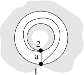
Figure 6.3. Triangulated annulus

Cutting the triangulation along an arc $\alpha$ corresponding to one of the ends of a double arrow we get a disk. Since the diagram of the new surface is a subdiagram of ${\mathcal{G}}$ obtained by removing the vertex corresponding to $\alpha$, this implies that

• ${\mathcal{G}}$ contains at most one double arrow;

• ${\mathcal{G}}$ looks like one of two diagrams shown in Figure 6.4.

Figure 6.4. Block decomposition of diagrams of type $\widetilde{A}_{p,q}$ containing a double arrow.

In particular, since ${\mathcal{P}}$ is either a cycle or a pseudo-cycle of type $\widetilde{A}_{2,2}$ (as no other pseudo-cycle from Table 4.1 is a subdiagram of a diagram of type $\widetilde{A}_{p,q}$) and $x$ is connected to ${\mathcal{P}}$ by at least two arrows, every risk diagram is contained in a subdiagram of type $A_{l}$. So, by Lemma 6.8 and results of [BM] we see that (C2) holds for all risk diagrams for ${\mathcal{G}}$.

Now, suppose that ${\mathcal{G}}$ contains simple arrows only. In this case any pseudo-cycle is an oriented cycle ${\mathcal{C}}$. If $|{\mathcal{C}}|>4$ then the triangulated surface corresponding to ${\mathcal{C}}$ has a puncture (since the only decomposition of ${\mathcal{C}}$ in this case consists of blocks of type I), which is impossible for ${\mathcal{C}}$ being a subdiagram of a diagram of type $\widetilde{A}_{p,q}$. If $|{\mathcal{C}}|\leq 4$ then the decomposability of $x\cup{\mathcal{P}}$ implies that $x\cup{\mathcal{P}}$ is one of the diagrams shown in Fig. 6.5; three of them can not be a subdiagram of a diagram of the type $\widetilde{A}_{p,q}$ since the corresponding surfaces have punctures, and the fourth is treated in Lemma 6.14.

∎

Figure 6.5. Small diagrams for the proof of Lemma 6.15: the diagram on the left is mutation-equivalent to $D_{4}$, the two diagrams on the right are mutation-equivalent to $\widetilde{D}_{4}$; the remaining one is checked in Lemma 6.14.

6.5. Condition (C2) for $\widetilde{D}_{n}$

All the risk diagrams in this section are subdiagrams of a diagram ${\mathcal{G}}$ of type $\widetilde{D}_{n}$.

Lemma 6.16.

Condition (C2) holds for three risk diagrams ${\mathcal{R}}=x\cup{\mathcal{P}}$ shown in Fig. 6.6.

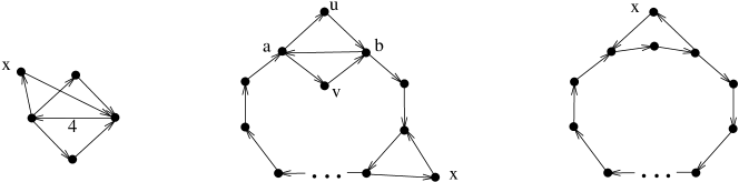
Figure 6.6. The diagrams in Lemma 6.16. The diagram in the middle has any size $|S|\geq 6$, the node $x$ is attached to the ends of any arrow not lying in the subdiagram $uvab$. The diagram on the right has any size $|S|\geq 5$.

The proof is straightforward.

Lemma 6.17.

Condition (C2) holds for all risk diagrams ${\mathcal{R}}=x\cup{\mathcal{P}}\subset{\mathcal{G}}$ where ${\mathcal{G}}$ is mutation-equivalent to $\widetilde{D}_{n}$.

Proof.

Recall that diagrams of type $\widetilde{D}_{n}$ correspond to ideal triangulations of a twice punctured disk (with $n-2$ marked points on the boundary).

Figure 6.7. Triangulation of a twice punctured disk and its diagram. $X$ is a diagram of type $A_{n-3}$.

First, suppose that ${\mathcal{G}}$ contains a double arrow. As it is shown in Table 3.1, a double arrow in a diagram of the type $\widetilde{D}_{n}$ can be obtained by gluing blocks of type II and IV only. The gluing of these two blocks results in a disk with two punctures and one marked point on the boundary, as shown in Fig. 6.7(a) (denote this disk by $\mathcal{A}$ and the whole twice punctured disk corresponding to the whole diagram ${\mathcal{G}}$ by $\mathcal{D}$). Clearly, $\mathcal{G}\setminus\mathcal{A}$ is a disk (corresponding to a diagram of type $A_{n-3}$, so the diagram ${\mathcal{G}}$ is constructed as in Fig. 6.7(b). In particular, this means that each risk diagram is either contained in a subdiagram of type $A_{k}$, or is one shown in Fig. 6.6 on the left. Thus, each risk subdiagram of ${\mathcal{G}}$ is already checked either in [BM] or in Lemma 6.16.

Figure 6.8. (a),(b): possible neighborhoods of a puncture (up to flip in an interior edge of the digon in (b)); (c),(d): the same with disks attached (also up to a flip in (d)); (e),(f): the corresponding diagrams (up to mutation in the vertices $v$ and $u$); diagrams marked by $A$ all have types $A_{k_{i}}$.

Now, suppose that ${\mathcal{G}}$ contains simple arrows only. Consider a puncture $p$ inside the twice punctured disk, let $\mathcal{U}$ be the union of all triangles incident to $p$. Then $\mathcal{U}$ is triangulated in one of the two ways shown in Fig. 6.8(a) and (b). The remaining part $\mathcal{D}\setminus\mathcal{U}$ of the twice punctured disk $\mathcal{D}$ is attached to $\mathcal{U}$ in such a way that either only one new puncture arises (for the diagram on Fig. 6.8(a)) or no new puncture arises (for the diagram of Fig. 6.8(b)). This is possible only if we attach some disks (or nothing at all) to some boundary edges of $\mathcal{U}$, which results in the triangulations looking as in Fig. 6.8(c) and (d) respectively, and corresponds to diagrams on Fig. 6.8(e) and (f). It is easy to see from these diagrams that all risk subdiagrams of ${\mathcal{G}}$ are already checked either in [BM] or in Section 6.4 or in Lemma 6.16.

∎

6.6. Condition (C2) for $\widetilde{B}_{n}$ and $\widetilde{C}_{n}$

Lemma 6.18.

Condition (C2) holds for the risk diagram ${\mathcal{R}}=x\cup{\mathcal{P}}$ shown in Fig. 6.9.

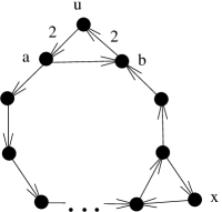
Figure 6.9. The diagram in Lemma 6.18. The diagram has any size $|{\mathcal{R}}|\geq 5$. The node $x$ is attached to the ends of any arrow not lying in the subdiagram $uab$.

The proof is straightforward.

Lemma 6.19.

Condition (C2) holds for all risk diagrams ${\mathcal{R}}=x\cup{\mathcal{P}}\subset{\mathcal{G}}$ where ${\mathcal{G}}$ is mutation-equivalent to $\widetilde{B}_{n}$ or $\widetilde{C}_{n}$.

Proof.

The diagrams of type $\widetilde{B}_{n}$ and $\widetilde{C}_{n}$ correspond to ideal triangulations of a punctured disk with one orbifold point and a disk with two orbifold points respectively, see Table 2.4.

First, suppose that ${\mathcal{G}}$ contains a double arrow. A double arrow is either contained in a block $\widetilde{\rm{V}}_{12}$ or is obtained by gluing two blocks of types II and $\widetilde{\rm{IV}}$, see Table 3.1. In the former case the triangulation looks as in Fig. 6.10(a) and the diagram ${\mathcal{G}}$ looks as in Fig. 6.10(b), so ${\mathcal{G}}$ does not contain any risk diagrams that were not studied yet. In the latter case we obtain the triangulation shown in Fig. 6.10(c) which results in a diagram shown in Fig. 6.10(d). Hence, each risk subdiagram of ${\mathcal{G}}$ is already checked either in [BM] or in Sections 6.4 and 6.5 or in Lemma 6.9.

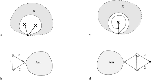
Figure 6.10. Diagrams of type $\widetilde{B}_{n}$ and $\widetilde{C}_{n}$ with double arrows. $X$ is a disk.

Suppose now that ${\mathcal{G}}$ contains no double arrows. Then any pseudo-cycle contained in ${\mathcal{G}}$ is either a simply-laced cycle or a pseudo-cycle of type $\widetilde{D}_{k}$ or $\widetilde{B}_{k}$. Consider these three types of pseudo-cycles separately.

A pseudo-cycle of type $\widetilde{D}_{k}$ can not be a subdiagram of ${\mathcal{G}}$ as the triangulated surface corresponding to $\widetilde{D}_{k}$ has two punctures, while the surface corresponding to ${\mathcal{G}}$ has either one puncture (if ${\mathcal{G}}$ is of type $\widetilde{B}_{n}$) or no punctures (if ${\mathcal{G}}$ is of type $\widetilde{C}_{n}$).

A pseudo-cycle of type $\widetilde{B}_{k}$ corresponds to a triangulated disk with a puncture and an orbifold point, so, it can not be a subdiagram of ${\mathcal{G}}$ if ${\mathcal{G}}$ is of mutation type $\widetilde{C}_{n}$. If ${\mathcal{G}}$ is of mutation type $\widetilde{B}_{n}$ then the triangulation of a surface corresponding to ${\mathcal{G}}$ is obtained from a triangulation of a surface corresponding to ${\mathcal{P}}$ by attaching a number of disks (see Fig. 6.11(a)), and the diagram ${\mathcal{G}}$ looks as in Fig. 6.11.b. The only new risk subdiagram in ${\mathcal{G}}$ is the diagram checked in Lemma 6.18.

Finally, consider a pseudo-cycle ${\mathcal{P}}$ which is a simply-laced cycle. Let ${\mathcal{R}}=x\cup{\mathcal{P}}$ be a risk diagram for ${\mathcal{G}}$. Consider a block decomposition of ${\mathcal{R}}$. If all arrows incident to $x$ in ${\mathcal{R}}$ are simple, then ${\mathcal{R}}$ is a skew-symmetric block-decomposable diagram and is already checked either in [BM] or in Sections 6.4 and 6.5. So, we may assume that some arrow incident to $x$ is labeled by $2$. Furthermore, since $x$ is attached to ${\mathcal{P}}$ by at least 2 arrows (by the definition of risk diagram), all blocks containing $x$ have at least two white vertices. The only block containing a non-simple arrow and two white vertices is the block $\widetilde{\rm{IV}}$. So, $x$ is attached to the simply-laced cycle ${\mathcal{P}}$ by the block $\widetilde{\rm{IV}}$ and we get a diagram shown in Fig. 6.11(c). After mutation in $x$ this diagram coincides with a pseudo-cycle of type $B_{k}$, so, (C2) for ${\mathcal{R}}$ becomes (C1) for pseudo-cycle of type $B_{k}$ which is already verified (See Cor. 6.12).

∎

Figure 6.11. To the proof of Lemma 6.19

6.7. Condition (C2) for $\widetilde{G}_{2}$

This is a small diagram with a small mutation class, so we just check (C2) explicitly.

6.8. Condition (C2) for $\widetilde{F}_{4}$

Consider the mutation class of $\widetilde{F}_{4}$ (it consists of 59 diagrams). We need to find all pseudo-cycles and all risk diagrams.

First, consider proper subdiagrams. Let ${\mathcal{G}}$ be a diagram of type $\widetilde{F}_{4}$. Then each proper subdiagram $X\subset{\mathcal{G}}$ has order at most $4$ and contains no arrows labeled by $3$. Due to results of [FeSTu2], this implies that either $X$ is block-decomposable or $X$ is mutation-equivalent to $F_{4}$. All risk diagrams contained in diagrams of mutation type $F_{4}$ satisfy (C2) by results of [BM]. Any block-decomposable affine diagram is of one of the types $\widetilde{A}_{p,q}$, $\widetilde{B}_{n}$, $\widetilde{C}_{n}$ or $\widetilde{D}_{n}$, and thus all risk diagrams are already checked in the previous sections. Hence, (C2) for risk subdiagrams of order at most $4$ is verified.

Looking through the mutation class, we find a unique risk diagram of order $5$, see Fig. 6.12(a). We label by $x$ the vertex not lying in the pseudo-cycle of order 4 (so that ${\mathcal{R}}={\mathcal{P}}\cup x$ where ${\mathcal{R}}$ is the risk diagram and ${\mathcal{P}}$ is a pseudo-cycle). It is easy to see that the mutation $\mu_{x}$ turns ${\mathcal{R}}$ into the cyclic diagram on Fig. 6.12(b). This diagram is a pseudo-cycle checked in Lemma 6.11.

This proves that (C2) holds for all risk diagrams for $\widetilde{F}_{4}$.

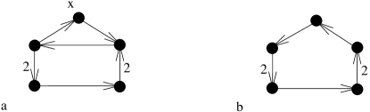
Figure 6.12. Risk diagram of order 5 for $\widetilde{F}_{4}$.

6.9. Condition (C2) for $\widetilde{E}_{6}$, $\widetilde{E}_{7}$, $\widetilde{E}_{8}$

Since $\widetilde{E}_{6}$, $\widetilde{E}_{7}$, $\widetilde{E}_{8}$ are skew-symmetric, the only types of pseudo-cycles we need to check are simply-laced oriented cycles and pseudo-cycles of types $\widetilde{A}_{p,q}$ and $\widetilde{D}_{k}$ . First we show (Lemma 6.20) that no sufficiently large risk diagram contains double arrow, then prove (Lemmas 6.21, 6.22 and 6.24) that the risk diagrams are block-decomposable, and finally, in Lemma 6.26 we show that (C2) holds for risk subdiagrams of diagrams of type $\widetilde{E}_{6}$, $\widetilde{E}_{7}$, $\widetilde{E}_{8}$.

Notation.

Given an arrow with ends $u$ and $v$ we will call it $uv$ if the arrow points to $v$.

Lemma 6.20.

Let ${\mathcal{P}}$ be an oriented cycle or a pseudo-cycle of type $\widetilde{D}_{k}$. Suppose that $|{\mathcal{P}}|>4$ and ${\mathcal{R}}=x\cup{\mathcal{P}}$ is a subdiagram of some mutation-finite skew-symmetric diagram $S$. Then ${\mathcal{R}}$ is simply-laced.

Proof.

First, we note that neither oriented cycles nor pseudo-cycles of type $\widetilde{D}_{k}$ contain double arrows if their order is more than $4$, so we need to show that $x$ is not attached to ${\mathcal{P}}$ by double arrow.

Suppose that $x$ is connected to ${\mathcal{P}}$ by a double arrow $xa$, $a\in{\mathcal{P}}$ (the case when the arrow $ax$ is not simple is similar). Let $b$ be a neighbor of $a$ in ${\mathcal{P}}$ such that ${\mathcal{P}}$ contains arrow $ba$ (such a neighbor exists since no pseudo-cycle of order at least $3$ contains a source). The subdiagram $U=\{xab\}\subset{\mathcal{R}}$ is a skew-symmetric mutation-finite diagram of order $3$ with a sink $a$. However, it is easy to check that any skew-symmetric mutation-finite diagram of order $3$ containing a double arrow is an oriented cycle. ∎

In the following three lemmas we show that for ${\mathcal{P}}$ either cyclic or of type $\widetilde{A}_{2,2}$ or $\widetilde{D}_{k}$ any risk diagram ${\mathcal{R}}=x\cup{\mathcal{P}}$ is block-decomposable.

Lemma 6.21.

Let ${\mathcal{P}}$ be a pseudo-cycle of the type $\widetilde{A}_{2,2}$ or $\widetilde{D}_{4}$. Suppose that ${\mathcal{R}}=x\cup{\mathcal{P}}$ is a mutation-finite skew-symmetric risk diagram. Then ${\mathcal{R}}$ is block-decomposable.

Proof.

The diagram ${\mathcal{R}}=x\cup{\mathcal{P}}$ is a mutation-finite skew-symmetric diagram of order 5 or 6, so to prove that it is block-decomposable one needs to show that it is not mutation-equivalent to $E_{6}$ or $X_{6}$ which is evident for $\widetilde{A}_{2,2}$ and can be done easily for $\widetilde{D}_{4}$.

∎

Lemma 6.22.

Let ${\mathcal{P}}$ be an oriented simply-laced cycle. Suppose that ${\mathcal{R}}=x\cup{\mathcal{P}}$ is a simply-laced risk diagram, and ${\mathcal{R}}$ is mutation-finite. Then ${\mathcal{R}}$ is block-decomposable.

Proof.

Let ${\mathcal{P}}=\{a_{1},\dots,a_{n}\}$ where $a_{i}$ is connected to $a_{i+1}$ by an arrow pointing to $a_{i+1}$ (with assumption $a_{n+1}=a_{1}$). Note that we may assume that $n\geq 5$: all skew-symmetric mutation-finite diagrams of order less than six are block-decomposable.

By the definition of risk diagram, $x$ is connected to ${\mathcal{P}}$ by both incoming and outgoing arrows. Without loss of generality we may assume that ${\mathcal{R}}$ contains an arrow $xa_{1}$, see Fig. 6.13(a). If $a_{2}x$ is the only other arrow incident to $x$ then ${\mathcal{P}}\cup x$ is clearly decomposable (into block $a_{1}a_{2}x$ of type II and others of type I, see Fig. 6.13(b)), so we assume that ${\mathcal{R}}$ contains some arrows $a_{i}x$ for $i>2$. Then there exists a unique cycle ${\mathcal{C}}$ containing $x,a_{1}$ and $a_{n}$, and this cycle is non-oriented. By Lemma 3.4, this implies that each vertex of ${\mathcal{P}}$ is connected to ${\mathcal{C}}$ by even number of arrows. Let $l=\min\{i\ |\ a_{i}\in{\mathcal{C}},i>1\}$. By assumption, $l>2$ , and there is one of the arrows $xa_{l}$ or $a_{l}x$.

If $l=3$ then $a_{2}$ is not connected to $x$ (otherwise there is an odd number of arrows connecting $a_{2}$ and ${\mathcal{C}}$). Thus, $a_{3}$ is connected to $x$ by the arrow $a_{3}x$ (since it is the only incoming arrow for $x$, see Fig. 6.13(c)), and this diagram is clearly block-decomposable (into blocks $xa_{1}a_{2}$, $xa_{2}a_{3}$ and $a_{i}a_{i+1}$ for $3\leq i\leq n$).

If $3<l\leq n$ then there is an arrow $xa_{2}$ (or $a_{2}x$) and an arrow $xa_{l-1}$ (or $a_{l-1}x$), otherwise Lemma 3.4 does not hold for $a_{2}$ or $a_{l-1}$. By the same reason, none of $a_{i}$ (for $2<i<l-1$) is connected to $x$, see Fig. 6.13(d). This diagram satisfies Lemma 3.4 only if both triangles $xa_{1}a_{2}$ and $xa_{l-1}a_{l}$ are oriented, which implies that the diagram is block-decomposable (into these two blocks of type II and others of type I).

∎

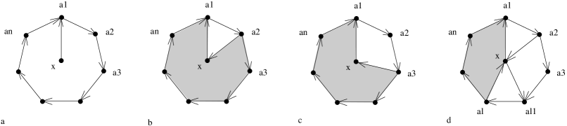
Figure 6.13. To the proof of Lemma 6.22

Remark 6.23.

Note that the block decomposition obtained in Lemma 6.22 consists of one or two blocks of type II containing $x$ and several blocks of type I; in particular, if a vertex $t$ of ${\mathcal{C}}$ is not connected to $x$ then it is contained in two blocks of type I.

Lemma 6.24.

Let ${\mathcal{P}}$ be a pseudo-cycle of the type $\widetilde{D}_{k},$ $k\geq 5$. Suppose that ${\mathcal{R}}=x\cup{\mathcal{P}}$ is a simply-laced risk diagram, and ${\mathcal{R}}$ is mutation-finite. Then ${\mathcal{R}}$ is block-decomposable.

Proof.

The pseudo-cycle ${\mathcal{P}}$ consists of a “big cycle” ${\mathcal{C}}$ with one arrow $ab$ reversed and two more vertices $u$ and $v$, see Fig. 6.14. The cycle ${\mathcal{C}}$ is non-oriented, so it is connected to $x$ by an even number $r$ of arrows.

Figure 6.14. To the proof of Lemma 6.24

First, suppose that $r=0$. Then both incoming to $x$ and outgoing from $x$ arrows belong to the subdiagram $xuv$. Then $xuav$ is a non-oriented cycle connected to $b$ by three arrows which is impossible by Lemma 3.4.

Now, suppose that $r>0$. As the next step of the proof, we want to show that $x\cup{\mathcal{C}}$ is block-decomposable. Then we will extend the block-decomposition of $x\cup{\mathcal{C}}$ to a block-decomposition of $x\cup{\mathcal{P}}$.

Claim: The subdiagram $x\cup{\mathcal{C}}$ is block-decomposable.

Proof of Claim.

Assume first that the only vertices of ${\mathcal{C}}$ connected to $x$ are $a$ and $b$. If the subdiagram $xab$ is a non-oriented cycle, then the subdiagram $xabc_{1}c_{k-3}$ is mutation-infinite [Kel], so we can assume that $xab$ is an oriented cycle. Then $x\cup{\mathcal{C}}$ can be decomposed into a block $xab$ of type II and others of type I.

Now assume that there is an arrow connecting $x$ and $c_{i}$. Then the proof follows the proof of Lemma 6.22 verbatim.

∎

To transform the decomposition of $x\cup{\mathcal{C}}$ to a decomposition of $x\cup{\mathcal{P}}$ we consider three cases: either $x$ is not connected to neither $a$ nor $b$, or $x$ is connected to exactly one of them, or it is connected to both. Our goal is to show that in all these cases the arrow $ab$ is a block of type I in a block decomposition of $x\cup{\mathcal{C}}$, and $x$ is connected to neither $u$ nor $v$: this means we can substitute $ab$ by a block $abuv$ of type IV to obtain a block decomposition of ${\mathcal{R}}$.

Case 1: $x$ is connected neither to $a$ nor to $b$.

First, we will show that $x$ is connected neither to $u$ nor to $v$.

Suppose the contrary. If $x$ is connected to both $u$ and $v$ then $avxu$ is a non-oriented cycle connected to $b$ by three arrows, which is impossible by Lemma 3.4, see Fig. 6.15(a). So, suppose that $x$ is connected to one of $u$ and $v$, say to $v$. Recall that $x$ is connected to ${\mathcal{P}}$ by at least two arrows. Since $x$ is not connected to $a,b,u$ we conclude that there exists $t\in{\mathcal{C}}$ such that $t$ is connected to $x$ (see Fig. 6.15(b)). Denote by ${\mathcal{C}}_{a}$ and ${\mathcal{C}}_{b}$ the subdiagrams in $x\cup{\mathcal{P}}$ such that ${\mathcal{C}}_{a}$ and ${\mathcal{C}}_{b}$ are chordless cycles containing $x$, $v$ and either $a$ or $b$ respectively. Clearly, at least one of ${\mathcal{C}}_{a}$ and ${\mathcal{C}}_{b}$ is non-oriented. On the other hand, $u$ is connected to each of ${\mathcal{C}}_{a}$ and ${\mathcal{C}}_{b}$ by a unique arrow, so we come to a contradiction.

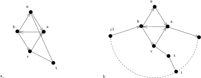
Figure 6.15. To the proof of Lemma 6.24, Case 1.

Therefore, we can transform the decomposition of $x\cup C$ into a decomposition of $x\cup{\mathcal{P}}$ by substituting a block $ab$ of type I (see Remark 6.23) by a block $abuv$ of type IV.

Case 2: $x$ is connected to exactly one of $a$ and $b$, say $a$ (the case when $x$ is connected to $b$ can be obtained by changing directions of all arrows).

Suppose first that $x$ is connected in ${\mathcal{C}}\setminus a$ to $c_{1}$ only (see Fig 6.16(a)). Then the cycle $xac_{1}$ is oriented (since $b$ is attached to it by one arrow only), and $ab$ is a block of type I in the block decomposition of $x\cup{\mathcal{C}}$. Let us show that $x$ is connected neither to $u$ nor to $v$, so $ab$ can be substituted by a block $abuv$ of type IV to produce a block decomposition of ${\mathcal{R}}$. Indeed, if $x$ is joined with both $u$ and $v$, then $c_{k-3}$ is connected to a non-oriented cycle $xubv$ by one arrow, which contradicts Lemma 3.4; if $x$ is joined with one of $u$ and $v$ (say $u$), then $v$ is connected to a non-oriented cycle $xua$ by exactly one arrow, which also leads to a contradiction.

Now assume that $x$ is connected to some $c_{i},\ i>1$ in ${\mathcal{C}}\setminus a$. Let $xabc_{k-3}\dots c_{m}$ be the smallest chordless cycle in $x\cup{\mathcal{C}}$ containing $xab$ (it clearly does exist in this case). Note that the cycle $xabc_{k-3}\dots c_{m}$ is non-oriented (see Fig 6.16(b)), so each of $u$ and $v$ is connected to it by even number of arrows. This implies that $x$ is not connected neither to $u$ nor to $v$. Furthermore, since $b$ is not connected to $x$, the arrow $ab$ in the decomposition of $x\cup{\mathcal{C}}$ is represented by a block of type I. Substituting this block by a block of type IV we obtain a block decomposition of ${\mathcal{R}}$.

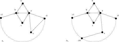
Figure 6.16. To the proof of Lemma 6.24, Case 2.

Case 3: $x$ is connected to both $a$ and $b$.

An application of Lemma 3.4 to any simply-laced diagram whose underlying graph is the complete graph on four vertices shows that such a diagram is mutation-infinite. Therefore, considering the subdiagrams $xabu$ and $xabv$ we conclude that $x$ is connected neither to $u$ nor to $v$. Thus, the subdiagram $xabuv$ looks as shown in Fig. 6.17(a).

Since the diagram shown in Fig. 6.17(b) is mutation-infinite for all directions of arrows incident to $x$, we conclude that $x$ is connected to $c_{1}$ and $c_{k-3}$, see Fig. 6.17(c). Furthermore, the cycle $bxc_{k-3}$ is oriented, since $u$ is connected to $bxc_{k-3}$ by a unique arrow. Similarly, the cycle $axc_{1}$ is oriented, which defines the directions of all arrows in $x\cup{\mathcal{P}}$. Note that $x$ is not connected to other $c_{i}\in{\mathcal{C}}$: in that case either $c_{1}$ or $c_{k-3}$ would be connected to a non-oriented cycle by a unique arrow in contradiction with Lemma 3.4. Now a block decomposition of ${\mathcal{R}}$ can be obtained in the same way as in the previous cases, see Fig. 6.17(d).

∎

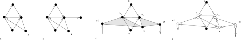
Figure 6.17. To the proof of Lemma 6.24, Case 3.

We summarize the results of Lemmas 6.20–6.24 in the following corollary.

Corollary 6.25.

Let ${\mathcal{P}}$ be a simply-laced oriented cycle or a pseudo-cycle of type $\widetilde{A}_{2,2}$ or $\widetilde{D}_{k}$. Let ${\mathcal{R}}={\mathcal{P}}\cup x$ be a mutation-finite skew-symmetric risk diagram. Then ${\mathcal{R}}$ is block-decomposable.

Lemma 6.26.

Condition (C2) holds for all risk diagrams of types $\widetilde{E}_{n}$, $n=6,7,8$.

Proof.

By Lemma 2.3, any risk subdiagram of $\widetilde{E}_{n}$ is either of finite or of affine type. By Corollary 6.25, all these risk subdiagrams are block-decomposable. So, any risk diagram is a block-decomposable skew-symmetric diagram of finite or affine type, i.e. any risk diagram is of mutation type $A_{k}$, $D_{k}$, $\widetilde{A}_{p,q}$ or $\widetilde{D}_{k}$ and is already checked in [BM] or in Sections 6.4 and 6.5. Therefore, (C2) holds for these risk diagrams.

∎

We verified conditions (C1) and (C2) for all pseudo-cycles and risk diagrams for all affine diagrams. By Lemma 6.5, this completes the proof of Theorem 4.7.

7. Examples of non-isomorphic groups $W$ and $\widetilde{W}_{{\mathcal{G}}}$

In this section, we show that for every affine Weyl group $W$ except $\widetilde{C}_{n}$ and $\widetilde{A}_{p,1}$ (cf. Remark 4.8) the relations of type (R4) (additional affine relations) are essential.

Recall that the group $\widetilde{W}_{{\mathcal{G}}}$ is obtained from $W_{{\mathcal{G}}}$ by omitting additional affine relations of type (R4).

Our aim is to prove that $\widetilde{W}_{{\mathcal{G}}}$ is not invariant under mutations. More precisely, we prove the following lemma.

Lemma 7.1.

Let ${\mathcal{G}}$ be one of the diagrams shown in Table 4.1, and let $W$ be the corresponding group from the right column of the table. Then $\widetilde{W}_{{\mathcal{G}}}$ is not isomorphic to $W$.

Here is the plan of the proof. By Lemma 4.6, there is a surjective homomorphism $\varphi:\widetilde{W}_{{\mathcal{G}}}\to W$. Our aim is to prove that $\varphi$ is not an isomorphism. According to Malcev [M, Theorem XII], this will imply that $\widetilde{W}_{{\mathcal{G}}}$ is not isomorphic to $W$ as soon as $W$ is a finitely generated linear group, which is of course true for Coxeter groups.

To show that $\varphi$ is not an isomorphism, we consider quotient groups $\widetilde{W}_{{\mathcal{G}}}/H$ and $W/\varphi(H)$, where $H$ is the normal closure of a suitable element of $\widetilde{W}_{{\mathcal{G}}}$, and see that these groups are not isomorphic.

We deal with all the diagrams separately.

7.1. ${\mathbf{W=\widetilde{A}_{3}}}$,

$${\mathcal{G}}=\raisebox{-22.76228pt}{\psfig{width=56.37271pt}}$$

Here

$$\widetilde{W}_{{\mathcal{G}}}=\langle t_{1},t_{2},t_{3},t_{4}\,|\,t_{i}^{2}=(t_{1}t_{2})^{3}=(t_{2}t_{3})^{3}=(t_{3}t_{4})^{3}=(t_{4}t_{1})^{3}=(t_{2}t_{4})^{2}=(t_{3}t_{2}t_{1}t_{2})^{3}=(t_{3}t_{4}t_{1}t_{4})^{3}=e\rangle,$$

$$W=\langle s_{1},s_{2},s_{3},s_{4}\,|\,s_{i}^{2}=(s_{1}s_{2})^{3}=(s_{2}s_{3})^{3}=(s_{3}s_{4})^{3}=(s_{4}s_{1})^{3}=(s_{2}s_{4})^{2}=(s_{1}s_{3})^{2}=e\rangle,$$

the epimorphism $\varphi:\widetilde{W}_{{\mathcal{G}}}\to W$ is defined by

$$\varphi(t_{1})=s_{1},\ \varphi(t_{2})=s_{2},\ \varphi(t_{3})=s_{4}s_{2}s_{3}s_{2}s_{4},\ \varphi(t_{4})=s_{4}$$

Now consider the normal closure $H=\langle t_{2}t_{4}\rangle^{\widetilde{W}_{{\mathcal{G}}}}$. Then the quotient group

$$\widetilde{W}_{{\mathcal{G}}}/H\cong\langle t_{1},t_{2},t_{3}\,|\,t_{i}^{2}=(t_{1}t_{2})^{3}=(t_{2}t_{3})^{3}=(t_{3}t_{2}t_{1}t_{2})^{3}=e\rangle\cong\widetilde{A}_{2},$$

and

$$W/\varphi(H)=\langle s_{1},s_{2},s_{3}\,|\,s_{i}^{2}=(s_{1}s_{2})^{3}=(s_{2}s_{3})^{3}=(s_{1}s_{3})^{2}=e\rangle\cong A_{3}$$

which are clearly not isomorphic.

7.2. ${\mathbf{W=\widetilde{D}_{n}}}$,

$${\mathcal{G}}=\raisebox{-31.2982pt}{\psfig{width=86.72267pt}}$$

$$\widetilde{W}_{{\mathcal{G}}}=\langle t_{1},\dotsm,t_{n+1}\,|\,t_{i}^{2}=(t_{i}t_{i+1})^{3}=(t_{1}t_{n})^{3}=(t_{2}t_{n+1})^{3}=(t_{2}t_{n})^{3}=(t_{i}t_{j})^{2}\,({\text{otherwise}})=\\ =(t_{1}t_{2}t_{n}t_{2})^{2}=(t_{n+1}t_{2}t_{n}t_{2})^{2}=e\rangle,$$

$$W\!=\!\langle s_{1},\dots,s_{n+1}\,|\,s_{i}^{2}=(s_{1}s_{2})^{3}\!=\dots=(s_{n-2}s_{n-1})^{3}\!=(s_{2}s_{n+1})^{3}\!=(s_{n-2}s_{n})^{3}\!=(s_{i}s_{j})^{2}\,({\text{otherwise}})=e\rangle,$$

the epimorphism $\varphi:\widetilde{W}_{{\mathcal{G}}}\to W$ is defined by

$$\varphi(t_{i})=s_{i},\ {\text{for }}i\neq n,\qquad\varphi(t_{n})=s_{n+1}s_{1}s_{2}\cdots s_{n-2}s_{n}s_{n-2}s_{n-3}\cdots s_{1}s_{n+1}$$

Take $H=\langle t_{1}t_{n+1}\rangle^{\widetilde{W}_{{\mathcal{G}}}}$. Then the quotient group

$$\widetilde{W}_{{\mathcal{G}}}=\langle t_{1},\dotsm,t_{n}\,|\,t_{i}^{2}=(t_{i}t_{i+1})^{3}=(t_{1}t_{n})^{3}=(t_{2}t_{n})^{3}=(t_{i}t_{j})^{2}\,({\text{otherwise}})=(t_{1}t_{2}t_{n}t_{2})^{2}=e\rangle\cong\widetilde{A}_{n-1},$$

while

$$W/\varphi(H)=\langle s_{1},\dots,s_{n}\,|\,s_{i}^{2}=(s_{1}s_{2})^{3}=\dots=(s_{n-2}s_{n-1})^{3}=(s_{n-2}s_{n})^{3}=(s_{i}s_{j})^{2}\,({\text{otherwise}})=e\rangle\cong D_{n}$$

7.3. ${\mathbf{W=\widetilde{B}_{3}}}$,

$${\mathcal{G}}=\raisebox{-22.76228pt}{\psfig{width=56.37271pt}}$$

Here

$$\widetilde{W}_{{\mathcal{G}}}=\langle t_{1},t_{2},t_{3},t_{4}\,|\,t_{i}^{2}=(t_{1}t_{2})^{4}=(t_{2}t_{3})^{4}=(t_{3}t_{4})^{3}=(t_{4}t_{1})^{3}=(t_{2}t_{4})^{2}=(t_{1}t_{2}t_{3}t_{2})^{2}=(t_{3}t_{4}t_{1}t_{4})^{3}=e\rangle,$$

$$W=\langle s_{1},s_{2},s_{3},s_{4}\,|\,s_{i}^{2}=(s_{1}s_{4})^{3}=(s_{2}s_{4})^{4}=(s_{3}s_{4})^{3}=(s_{1}s_{2})^{3}=(s_{2}s_{3})^{2}=(s_{1}s_{3})^{2}=e\rangle,$$

the epimorphism $\varphi:\widetilde{W}_{{\mathcal{G}}}\to W$ is defined by

$$\varphi(t_{1})=s_{2}s_{4}s_{1}s_{4}s_{2},\ \varphi(t_{2})=s_{2},\ \varphi(t_{3})=s_{4}s_{3}s_{4},\ \varphi(t_{4})=s_{3}$$

Now take $H=\langle(t_{2}t_{3})^{2}\rangle^{\widetilde{W}_{{\mathcal{G}}}}$. Then the quotient group

$$\widetilde{W}_{{\mathcal{G}}}=\langle t_{1},t_{2},t_{3},t_{4}\,|\,t_{i}^{2}=(t_{1}t_{2})^{4}=(t_{2}t_{3})^{2}=(t_{3}t_{4})^{3}=(t_{4}t_{1})^{3}=(t_{2}t_{4})^{2}=(t_{1}t_{3})^{2}=e\rangle\cong B_{4},$$

while

$$W/\varphi(H)=\langle s_{1},s_{2},s_{3},s_{4}\,|\,s_{i}^{2}=(s_{1}s_{4})^{3}=(s_{2}s_{4})^{2}=(s_{3}s_{4})^{3}=(s_{1}s_{2})^{3}=(s_{2}s_{3})^{2}=(s_{1}s_{3})^{2}=e\rangle\cong A_{1}\times A_{3}$$

7.4. ${\mathbf{W=\widetilde{B}_{n}}}$,

$${\mathcal{G}}=\raisebox{-22.76228pt}{\psfig{width=99.73074pt}}$$

$$\widetilde{W}_{{\mathcal{G}}}=\langle t_{1},\dotsm,t_{n+1}\,|\,t_{i}^{2}=(t_{n+1}t_{1})^{4}=(t_{n+1}t_{n})^{4}=(t_{1}t_{2})^{3}=(t_{2}t_{3})^{3}=\dots=(t_{n-1}t_{n})^{3}=\\ =(t_{n}t_{1})^{3}=(t_{i}t_{j})^{2}\,({\text{otherwise}})=(t_{n+1}t_{1}t_{n}t_{1})^{2}=e\rangle,$$

$$W=\langle s_{1},\dots,s_{n+1}\,|\,s_{i}^{2}=(s_{n+1}s_{1})^{4}=(s_{1}s_{2})^{3}=(s_{2}s_{3})^{3}=\dots=(s_{n-2}s_{n-1})^{3}=\\ =(s_{n-2}s_{n})^{3}=(s_{i}s_{j})^{2}\,({\text{otherwise}})=e\rangle,$$

similarly to the case of $\widetilde{D}_{n}$, the epimorphism $\varphi:\widetilde{W}_{{\mathcal{G}}}\to W$ is defined by

$$\varphi(t_{i})=s_{i},\ {\text{for }}i\neq n,\qquad\varphi(t_{n})=s_{n+1}s_{1}s_{2}\cdots s_{n-2}s_{n}s_{n-2}s_{n-3}\cdots s_{1}s_{n+1}$$

Take $H=\langle(t_{1}t_{n+1})^{2}\rangle^{\widetilde{W}_{{\mathcal{G}}}}$. Then the quotient group

$$\widetilde{W}_{{\mathcal{G}}}=\langle t_{1},\dotsm,t_{n}\,|\,t_{i}^{2}=(t_{n+1}t_{n})^{4}=(t_{1}t_{2})^{3}=(t_{2}t_{3})^{3}=\dots=(t_{n-1}t_{n})^{3}=(t_{i}t_{j})^{2}\,({\text{otherwise}})=e\rangle\cong\widetilde{B}_{n+1},$$

while

$$W/\varphi(H)=\langle s_{1},\dots,s_{n+1}\,|\,s_{i}^{2}=(s_{n+1}s_{1})^{2}=(s_{1}s_{2})^{3}=(s_{2}s_{3})^{3}=\dots=(s_{n-2}s_{n-1})^{3}=\\ =(s_{n-2}s_{n})^{3}=(s_{i}s_{j})^{2}\,({\text{otherwise}})=e\rangle\cong B_{n}\times A_{1}$$

7.5. ${\mathbf{W=\widetilde{G}_{2}}}$,

$${\mathcal{G}}=\raisebox{-17.07182pt}{\psfig{width=47.69846pt}}$$

Here

$$\widetilde{W}_{{\mathcal{G}}}=\langle t_{1},t_{2},t_{3}\,|\,t_{i}^{2}=(t_{1}t_{2})^{6}=(t_{1}t_{3})^{6}=(t_{1}t_{2}t_{3}t_{2})^{6}=(t_{2}t_{3}t_{1}t_{3})^{6}=(t_{3}t_{1}t_{2}t_{1})^{3}=e\rangle,$$

$$W=\langle s_{1},s_{2},s_{3},s_{4}\,|\,s_{i}^{2}=(s_{1}s_{3})^{6}=(s_{2}s_{3})^{3}=(s_{1}s_{2})^{2}=e\rangle,$$

the epimorphism $\varphi:\widetilde{W}_{{\mathcal{G}}}\to W$ is defined by

$$\varphi(t_{1})=s_{3}s_{1}s_{3},\ \varphi(t_{2})=s_{3}s_{1}s_{3}s_{2}s_{3}s_{1}s_{3},\ \varphi(t_{3})=s_{3}$$

Now take $H=\langle(t_{1}t_{3})^{2}\rangle^{\widetilde{W}_{{\mathcal{G}}}}$. Then the quotient group

$$\widetilde{W}_{{\mathcal{G}}}=\langle t_{1},t_{2},t_{3}\,|\,t_{i}^{2}=(t_{1}t_{2})^{6}=(t_{1}t_{3})^{2}=(t_{2}t_{3})^{3}=e\rangle\cong\widetilde{G}_{2},$$

while

$$W/\varphi(H)=\langle s_{1},s_{2},s_{3}\,|\,s_{i}^{2}=(s_{1}s_{3})^{2}=(s_{2}s_{3})^{3}=(s_{1}s_{2})^{2}=e\rangle\cong A_{1}\times A_{2}$$

8. Generalization for diagrams arising from unpunctured surfaces and orbifolds

Let ${\mathcal{G}}$ be a diagram arising from an unpunctured surface or orbifold. We construct a group $W_{{\mathcal{G}}}$ in the similar way as before (but with one more additional type of relations, see Section 8.1) and show that this group is invariant under mutations. In this case $W_{{\mathcal{G}}}$ is not a Coxeter group anymore, but a quotient of some Coxeter group (by relations of types (R3)–(R5), see below).

8.1. Construction of the group $W_{{\mathcal{G}}}$

Definition 8.1.

Given a diagram ${\mathcal{G}}$ of order $n$ arising from a triangulated unpunctured surface or orbifold, $W_{\mathcal{G}}$ is a group with

• generators $s_{1},\dots,s_{n}$ corresponding to the vertices of ${\mathcal{G}}$;

• relations:

  • $s_{i}^{2}=e$ for $i=1,\dots,n$;

  • $(s_{i}s_{j})^{m_{ij}}=e$ for all vertices $i$, $j$ not joined by an arrow labeled by $4$ (where $m_{ij}$ are defined in Section 4);

  • cycle relation for every chordless oriented cycle (see relations of type (R3) in Section 4);

  • four types of additional relations for affine diagrams from Table 4.1;

  • additional relations for a handle:

    $$(s_{1}s_{2}s_{3}s_{4}s_{3}s_{2})^{3}=e\text{\ and \ }(s_{1}s_{2}s_{3}s_{4}s_{5}s_{4}s_{3}s_{2})^{2}=e$$

    for all subdiagrams of type ${\mathcal{H}}_{0}$ and ${\mathcal{H}}$ shown in Fig. 8.1;

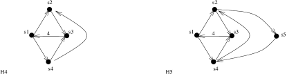
Figure 8.1. Additional relations: the diagram ${\mathcal{H}}$ corresponds to a handle with two marked points at the boundary component. The diagram ${\mathcal{H}}_{0}$ corresponds to a handle with one marked point (i.e., the boundary corresponds to vertex $5$ of ${\mathcal{H}}$).

Remark 8.2.

(i) Relations (R1)-(R4) are the same as in the construction of the group for the affine case.

(ii) The diagrams for relations (R5) correspond to a handle with one and two marked points at the boundary component.

(iii) The diagram ${\mathcal{H}}_{0}$ is a subdiagram of ${\mathcal{H}}$, and the relation (R5) for ${\mathcal{H}}_{0}$ is a corollary of the relation (R5) for ${\mathcal{H}}$. Furthermore, it is easy to observe that if the diagram ${\mathcal{H}}_{0}$ is a subdiagram of a bigger diagram $Q$ originating from a triangulation of a surface or orbifold, then there exists ${\mathcal{H}}\subset{\mathcal{Q}}$ containing ${\mathcal{H}}_{0}$. Together with the observation above this implies that the only diagram for which the first relation in (R5) needs to be applied is ${\mathcal{H}}_{0}$ itself.

(iii) The second relation (R5) is equivalent to any of the following three relations:

$$(s_{1}s_{4}s_{3}s_{2}s_{5}s_{2}s_{3}s_{4})^{2}=e,\qquad(s_{3}s_{2}s_{1}s_{4}s_{5}s_{4}s_{1}s_{2})^{2}=e,\qquad(s_{3}s_{4}s_{1}s_{2}s_{5}s_{2}s_{1}s_{4})^{2}=e.$$

8.2. Invariance of the group $W_{{\mathcal{G}}}$

Theorem 8.3.

Let ${\mathcal{G}}$ be a diagram arising from an unpunctured surface or orbifold, and let $W_{{\mathcal{G}}}$ be the group defined as above. Then $W_{{\mathcal{G}}}$ is invariant under mutations of ${\mathcal{G}}$.

Let us define pseudo-cycles and risk diagrams in the same way as for affine diagrams: pseudo-cycles are supports of relations (R1)–(R5), and risk diagrams are diagrams of the form $x\cup{\mathcal{P}}$, where ${\mathcal{P}}$ is a pseudo-cycle, and $x$ is connected to ${\mathcal{P}}$ by at least one incoming and one outgoing arrow.

Now note that the proofs of Lemmas 6.5 and 6.6 do not use the property of ${\mathcal{G}}$ to be of affine type. Therefore, to prove Theorem 8.3 we can use exactly the same strategy as in the affine case: we list all pseudo-cycles, find all risk subdiagrams for each of them and check conditions (C1) and (C2) of Lemma 6.5.

Lemma 8.4.

Let ${\mathcal{G}}$ be a diagram arising from a triangulated unpunctured surface. Then ${\mathcal{G}}$ contains no oriented chordless cycles of length bigger than 3.

Moreover, the same holds for diagrams arising from triangulated unpunctured orbifolds.

Proof.

First suppose that ${\mathcal{G}}$ comes from a triangulated surface. Then ${\mathcal{G}}$ is block-decomposable. Since the surface is unpunctured, the list of possible blocks in the decomposition is exhausted by blocks of type I and II (both corresponding to ordinary, non-self-folded triangles). If these blocks are arranged to make an oriented cycle (not composing a single block) then the corresponding triangles make a circular neighborhood of a common vertex (see Fig. 8.2), so this turns into a puncture which is not allowed by the assumption.

Now, suppose that ${\mathcal{G}}$ comes from a triangulated unpunctured orbifold. Then the block-decomposition of ${\mathcal{G}}$ consists of blocks of types I, II, $\widetilde{\rm{IV}}$ and $\widetilde{\rm{V}}_{12}$. Furthermore, if ${\mathcal{C}}\subset{\mathcal{G}}$ is an oriented cycle, then no block of type $\widetilde{V}_{12}$ has an arrow in ${\mathcal{C}}$ (since this block has only one white vertex). Let ${\mathcal{C}}^{\prime}$ be a subdiagram of ${\mathcal{G}}$ spanned by all blocks having an arrow in ${\mathcal{C}}$. Constructing a triangulation corresponding to ${\mathcal{C}}^{\prime}$ we get a puncture again, see Fig. 8.2.

∎

Figure 8.2. Lemma 8.4: A long oriented cycle in the diagram corresponds to a puncture on the surface/orbifold (some of the vertices or edges of the triangles in the figure may coincide).

In view of Lemma 8.4, any pseudo-cycle in ${\mathcal{G}}$ is either a subdiagram of order at most $3$, or of one of four additional (affine) types in Table 4.1, or the diagrams ${\mathcal{H}}_{0}$ and ${\mathcal{H}}$ in Fig. 8.1. Moreover, three of five additional affine types are diagrams of mutation type $\widetilde{D}_{n}$ or $\widetilde{B}_{n}$, thus ones arising from a punctured surface/orbifold. One is of mutation type $\widetilde{G}_{2}$, so does not arise from surfaces or orbifolds. Hence, in the unpunctured case we only need to check the following types of pseudo-cycles:

• two-vertex subdiagrams;

• oriented triangles;

• additional affine pseudo-cycle of mutation type $\widetilde{A}_{2,2}$;

• diagrams ${\mathcal{H}}_{0}$ and ${\mathcal{H}}$.

Lemma 8.5.

Condition (C1) of Lemma 6.5 holds for ${\mathcal{H}}_{0}$ and ${\mathcal{H}}$.

The proof of the lemma is straightforward. Together with the result of Lemma 6.9 the lemma implies that (C1) holds for all pseudo-cycles that can be found in a diagram arising from an unpunctured surface/orbifold.

Our next step is to find all risk diagrams for all pseudo-cycles.

Lemma 8.6.

Let ${\mathcal{G}}$ be a diagram arising from an unpunctured surface/orbifold, and let ${\mathcal{R}}$ be its risk subdiagram. Then ${\mathcal{R}}$ is either a risk diagram for some affine diagram, or ${\mathcal{R}}={\mathcal{H}}$ or ${\mathcal{R}}=\mu_{5}({\mathcal{H}})$ (where $\mu_{5}({\mathcal{H}})$ is the diagram on Fig. 8.3 obtained from ${\mathcal{H}}$ by one mutation).

Proof.

Let ${\mathcal{P}}$ be a pseudo-cycle and ${\mathcal{R}}=\!x\cup{\mathcal{P}}\!$. If ${\mathcal{P}}$ has two or three vertices we list all block-decomposable diagrams with 3 or 4 vertices respectively (and choose those of them having ${\mathcal{P}}$ as a subdiagram) and verify explicitly that they all appear as subdiagrams of diagrams of affine type.

For ${\mathcal{P}}$ of type $\widetilde{A}_{2,2}$ or of type ${\mathcal{H}}$ we note that ${\mathcal{P}}$ has an arrow labeled by $4$, so this arrow is obtained by gluing two blocks. Keeping in mind that ${\mathcal{R}}$ is block-decomposable and that the vertex $x$ of a risk diagram should be connected to ${\mathcal{P}}$ by both an incoming and an outgoing arrow, it is easy to see that the pseudo-cycle ${\mathcal{H}}$ does not belong to any risk diagram, and the pseudo-cycle $\widetilde{A}_{2,2}$ belongs to the risk diagram $\mu_{5}({\mathcal{H}})$ only.

Finally, for ${\mathcal{P}}$ of type ${\mathcal{H}}_{0}$, ${\mathcal{P}}$ is contained in ${\mathcal{H}}$ (see Remark 8.2(iii)), and the only vertex of ${\mathcal{G}}$ connected to vertices of ${\mathcal{P}}$ is the remaining vertex of ${\mathcal{H}}$: this can be easily seen from the block decomposition. This implies that the risk diagram coincides with ${\mathcal{H}}$.

∎

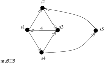
Figure 8.3. The diagram $\mu_{5}({\mathcal{H}})$ obtained by a mutation of ${\mathcal{H}}$.

Lemma 8.7.

Condition (C2) of Lemma 6.5 holds for all risk subdiagrams of diagrams arising from unpunctured surfaces and orbifolds.

Proof.

By Lemma 8.6, we only need to check risk diagrams of type ${\mathcal{H}}$ and $\mu_{5}({\mathcal{H}})$. Thus, (C2) for this risk diagram is already checked as (C1) for pseudo-cycle ${\mathcal{H}}$.

∎

Lemmas 8.5 and 8.7 imply Theorem 8.3.

Remark 8.8.

Unlike to the affine case, the group $W_{{\mathcal{G}}}$ for ${\mathcal{G}}$ arising from an unpunctured surface or orbifold is not a Coxeter group but a quotient of some Coxeter group.

Question 8.9.

(i) Given two mutationally non-equivalent diagrams ${\mathcal{G}}_{1}$ and ${\mathcal{G}}_{2}$ arising from (distinct) unpunctured surfaces or orbifolds, is it true that $W_{{\mathcal{G}}_{1}}$ is not isomorphic to $W_{{\mathcal{G}}_{2}}$?

(ii) What types of groups can be obtained as groups $W_{{\mathcal{G}}}$?

9. Exceptional diagrams

In this section, we construct the groups for the remaining exceptional mutation-finite diagrams, i.e. for diagrams which are neither block-decomposable nor of finite or affine type. By Theorem 2.5, these diagrams are exhausted by the following mutation types: $X_{6}$, $X_{7}$, $E_{6}^{(1,1)}$, $E_{7}^{(1,1)}$, $E_{8}^{(1,1)}$, $G_{2}^{(*,+)}$, $G_{2}^{(*,*)}$, $F_{4}^{(*,+)}$, $F_{4}^{(*,*)}$.

Definition 9.1 (Group $W_{\mathcal{G}}$ for exceptional diagrams).

Let ${\mathcal{G}}$ be a diagram of an exceptional mutation type. Define group $W_{\mathcal{G}}$ as the group with generators $s_{1},\dots,s_{n}$ corresponding to the vertices of ${\mathcal{G}}$ and with relations

• $s_{i}^{2}=e$ for $i=1,\dots,n$;

• $(s_{i}s_{j})^{m_{ij}}=e$ for all vertices $i$, $j$ not joined by an arrow labeled by $4$ (where $m_{ij}$ are defined in Section 4);

• cycle relation for every chordless oriented cycle (see relations of type (R3) in Section 4);

• (additional affine relations) for every subdiagram of ${\mathcal{G}}$ of the form shown in the first column of Table 4.1 we take the relations listed in the second column of the table;

• additional $X_{5}$-relation

  $$(s_{1}s_{0}s_{2}s_{0}s_{1}s_{3}s_{0}s_{4}s_{0}s_{3})^{2}=e$$

  for diagram $X_{5}$ shown in Fig. 9.1.

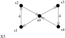
Figure 9.1. A diagram $X_{5}$.

Remark 9.2.

(i) For non-decomposable diagrams of finite or affine type the definition above coincides with ones from [BM] and Section 4.

(ii) The relation (R5*) is equivalent to $(s_{2}s_{0}s_{1}s_{0}s_{2}s_{4}s_{0}s_{3}s_{0}s_{4})^{2}=e$.

(iii) Relation (R5*) is necessary for mutation classes $X_{6}$ and $X_{7}$ only.

(iv) The diagram $X_{5}$ corresponds to a triangulated punctured annulus. We expect that relation (R5*) will lose its exceptional character when we will define the group $W_{\mathcal{G}}$ for surfaces with punctures.

Theorem 9.3.

If ${\mathcal{G}}$ is a diagram of the exceptional finite mutation type (i.e. ${\mathcal{G}}$ is mutation-equivalent to one of $X_{6},X_{7},E_{6}^{(1,1)},E_{7}^{(1,1)},E_{8}^{(1,1)},G_{2}^{(*,+)},G_{2}^{(*,*)},F_{4}^{(*,+)}$ or $F_{4}^{(*,*)}$) then the group $W_{{\mathcal{G}}}$ is invariant under mutations.

Note that, similarly to the groups constructed for surfaces or orbifolds, the groups obtained in the exceptional cases are quotients of Coxeter groups. We do not know whether these groups are distinct for different mutation classes or not.

To prove Theorem 9.3 we consider cases of $X_{n}$, $E_{n}^{(1,1)}$, $G_{2}^{(\cdot,\cdot)}$ and $F_{4}^{(\cdot,\cdot)}$ separately.

9.1. Groups for $X_{6}$ and $X_{7}$

The proof of the invariance of the group $W_{\mathcal{G}}$ under mutations is a straightforward check of pseudo-cycles and risk diagrams based on Lemma 6.5.

More precisely, first we check condition (C1) for the pseudo-cycle of type $X_{5}$. Then we check that there is no risk diagrams containing the pseudo-cycle $X_{5}$: we look through the mutation classes of $X_{6}$ and $X_{7}$ using the fact the they are small (containing 5 and 2 diagrams respectively). We also check that if ${\mathcal{R}}$ is a risk diagram containing some pseudo-cycle then either ${\mathcal{R}}$ is a risk diagram for some diagram of affine type or ${\mathcal{R}}=X_{5}$. Condition (C2) for risk subdiagrams of diagrams of affine type has already been checked above. (C2) for the risk diagram ${\mathcal{R}}=X_{5}$ is (C1) for the pseudo-cycle of type $X_{5}$.

9.2. Groups for diagrams $G_{2}^{(*,+)}$ and $G_{2}^{(*,*)}$

The proof of the invariance is a direct check due to small mutation classes (6 and 2 diagrams respectively).

9.3. Groups for diagrams $F_{4}^{(*,+)}$ and $F_{4}^{(*,*)}$

The mutation classes of $F_{4}^{(*,+)}$ and $F_{4}^{(*,*)}$ are rather large (90 and 35 diagrams respectively), so we use pseudo-cycles and risk diagrams.

More precisely, if ${\mathcal{P}}$ is a pseudo-cycle and it is not a subdiagram of any affine diagram, then ${\mathcal{P}}$ defines a relation of type (R3) (cyclic relation) and is one of the cycles listed in Table 3.2. There is a unique pseudo-cycle which is not a subdiagram of any affine diagram and does not contain arrows labeled by $3$, namely the cyclic diagram shown in row 10 of the table. A straightforward computation shows that (C1) holds for this pseudo-cycle.

Now, we need to list and check all risk diagrams.

Lemma 9.4.

Condition (C2) holds for all risk subdiagrams of $F_{4}^{(*,+)}$ and $F_{4}^{(*,*)}$.

Proof.

First, we do not need to check any decomposable risk diagrams (by results of Sections 6.4, 6.5 and 6.6) or subdiagrams of affine diagrams. This implies that we are not interested in risk diagrams of size smaller than 6 (since any diagram of size at most 5 and containing no arrows labeled by $3$ is either block-decomposable or a subdiagram of $\widetilde{F}_{4}$). So, we need to study risk diagrams of order 6 only, i.e. the diagrams mutation-equivalent to $F_{4}^{(*,+)}$ or $F_{4}^{(*,*)}$.

To check risk subdiagrams of order 6 we consider all pseudo-cycles of order 5 and add an additional vertex $x$ to them. There are 4 pseudo-cycles of order 5, namely a simply-laced cycle, the cyclic diagram of mutation type $\widetilde{F}_{4}$ (shown in row 9 of Table 3.2), and additional affine pseudo-cycles of types $\widetilde{D}_{4}$ and $\widetilde{B}_{4}$. For each pseudo-cycle ${\mathcal{P}}$ we add a vertex $x$ such that

• $x\cup{\mathcal{P}}$ is mutation-finite;

• $x$ is connected to ${\mathcal{P}}$ by at least one outgoing and at least one incoming arrow;

• $x\cup{\mathcal{P}}$ has at least one arrow labeled by $2$ (otherwise we get either block-decomposable diagram, or $E_{6}$ or $X_{6}$).

The mutation-finiteness of ${\mathcal{R}}=x\cup{\mathcal{P}}$ implies in particular that

• $x$ is connected to ${\mathcal{P}}$ by arrows labeled by $1$, $2$ or $4$ only;

• all non-oriented cycles in ${\mathcal{R}}$ are simply-laced (see Remark 9.5 below).

It turns out after a short case-by-case study that any mutation-finite diagram ${\mathcal{R}}=x\cup{\mathcal{P}}$ of the required type is either block-decomposable (which is not the case for the diagram of mutation type $F_{4}^{(*,+)}$ or $F_{4}^{(*,*)}$) or the diagram shown in Fig. 9.2. The mutation $\mu_{x}$ turns the latter diagram into the cyclic diagram of mutation type $F_{4}^{(*,+)}$ (row 10 in Table 3.2), so (C2) for this risk diagram was checked as a (C1) for the cyclic pseudo-cycle.

∎

Figure 9.2. To the proof of Lemma 9.4.

Remark 9.5.

It is an easy observation that all non-oriented mutation-finite cycles are simply-laced. In skew-symmetric case this was mentioned in [Se1].

9.4. Groups for diagrams $E_{6}^{(1,1)}$, $E_{7}^{(1,1)}$ and $E_{8}^{(1,1)}$

To check the invariance of the groups we consider pseudo-cycles and risk diagrams.

Lemma 9.6.

Conditions (C1) and (C2) hold for all pseudo-cycles and all risk diagrams of $E_{6}^{(1,1)}$, $E_{7}^{(1,1)}$ and $E_{8}^{(1,1)}$.

Proof.

Condition (C1) holds since we have not introduced any new pseudo-cycles (comparing to the affine case).

To prove that (C2) holds note that the diagrams $E_{6}^{(1,1)}$, $E_{7}^{(1,1)}$ and $E_{8}^{(1,1)}$ are skew-symmetric, which implies that any pseudo-cycle is of one of the following forms:

• a simply-laced cycle;

• a cycle of type $\widetilde{A}_{2,1}$ (row 1 in Table 3.2);

• an additional affine pseudo-cycle of type $\widetilde{A}_{2,2}$;

• an additional affine pseudo-cycle of type $\widetilde{D}_{n}$.

The risk diagrams containing pseudo-cycles of types $\widetilde{A}_{2,1}$ and $\widetilde{A}_{2,2}$ can be checked explicitly. The risk diagrams for a simply-laced cycle and an additional affine pseudo-cycle of type $\widetilde{D}_{n}$ are described in Remark 6.23 and also can be easily checked.

∎

This completes the proof of Theorem 9.3.

References

- [BCP] W. Bosma, J. J. Cannon, C. Playoust, The Magma algebra system. I. The user language, J. Symbolic Comput. 24 (1997), 235–265.
- [BM] M. Barot, R. J. Marsh, Reflection group presentations arising from cluster algebras, Trans. Amer. Math. Soc. 367 (2015), 1945–1967.
- [BMR] A. B. Buan, R. J. Marsh, I. Reiten, Cluster mutation via quiver representations, Comment. Math. Helv. 83 (2008), 143–177.
- [Fe] A. Felikson, Spherical simplices generating discrete reflection groups, Sb. Math. 195 (2004), 585–598.
- [FeSThTu] A. Felikson, M. Shapiro, H. Thomas, P. Tumarkin, Growth rate of cluster algebras, Proc. London Math. Soc. 109 (2014), 653–675.
- [FeSTu1] A. Felikson, M. Shapiro, P. Tumarkin, Skew-symmetric cluster algebras of finite mutation type, J. Eur. Math. Soc. 14 (2012), 1135–1180.
- [FeSTu2] A. Felikson, M. Shapiro, P. Tumarkin, Cluster algebras of finite mutation type via unfoldings, Int. Math. Res. Notices 8 (2012), 1768–1804.
- [FeSTu3] A. Felikson, M. Shapiro, P. Tumarkin, Cluster algebras and triangulated orbifolds, Adv. Math. 231 (2012), 2953–3002
- [FeTu] A. Felikson, P. Tumarkin, Coxeter groups, quiver mutations and geometric manifolds, arXiv:1409.3427
- [FST] S. Fomin, M. Shapiro, D. Thurston, Cluster algebras and triangulated surfaces. Part I: Cluster complexes, Acta Math. 201 (2008), 83–146.
- [FZ] S. Fomin, A. Zelevinsky, Cluster algebras II: Finite type classification, Invent. Math. 154 (2003), 63–121.
- [K] V. Kac, Infinite-dimensional Lie algebras, Cambridge Univ. Press, London, 1985.
- [Kel] B. Keller, Quiver mutation in Java, www.math.jussieu.fr/~keller/quivermutation
- [M] A. Malcev, On isomorphic matrix representations of infinite groups, Mat. Sb. 8 (1940), 405–422; Amer. Math. Soc. Transl. (2) 45 (1965), 1–18.
- [P] M. J. Parsons, Companion bases for cluster-tilted algebras, Algebr. Represent. Theory 17 (2014), 775–808.
- [Se1] A. Seven, Quivers of finite mutation type and skew-symmetric matrices, Linear Algebra Appl. 433 (2010), 1154–1169.
- [Se2] A. Seven, Reflection group relations arising from cluster algebras, arXiv:1210.6217
- [Z] B. Zhu, Preprojective cluster variables of acyclic cluster algebras, Comm. Algebra 35 (2007), 2857–2871.