More Evidence for the Intermediate Broad Line Region of the Mapped AGN PG 0052+251

Abstract

In the manuscript, the properties of the proposed intermediate BLR are checked for the mapped AGN PG 0052+251. With the considerations of the apparent effects of the broad He ii line on the observed broad H$\beta$ profile, the line parameters (especially the line width and the line flux) of the observed broad H$\alpha$ and the broad H$\beta$ are carefully determined. Based on the measured line parameters, the model with two broad components applied for each observed broad balmer line is preferred, and then confirmed by the calculated much different time lags for the inner/intermediate broad components and the corresponding virial BH masses ratio determined by the properties of the inner and the intermediate broad components. Then, the correlation between the broad line width and the broad line flux is checked for the two broad components: one clearly strong negative correlation for the inner broad component, but one positive correlation for the intermediate broad component. The different correlations for the two broad components strongly support the intermediate BLR of PG0052+251.

1 Introduction

PG 0052+251 is one well studied mapped blue quasar (Bentz et al. 2009, Chelouche & Daniel 2012, Collin et al. 2006, Kaspi et al. 2000, 2005, Peterson et al. 2004, Zu et al. 2011, Zhang 2011b). Based on the measured size of the BLR (Broad emission Line Region) and the line width of the broad $H\alpha$ and the broad H$\beta$ in the literature, we (Zhang 2011b, Paper I) have shown that the blue quasar PG 0052+251 is one special object in the plane of $(\frac{\sigma(H\beta)}{\sigma(H\alpha)})^{2}$ versus $\frac{R_{BLR,H\alpha}}{R_{BLR,H\beta}}$, where $\sigma$ and $R_{BLR}$ mean the measured broad line width based on the mean/rms spectra and the size of the BLR determined by the reverberation mapping technique (Blandford & Mckee 1992, Peterson 1993, Peterson & Horne 2004), because of the much different virial black hole masses determined by the parameters of the broad H$\beta$ and the broad H$\alpha$. So that, in the Paper I, we have reported that it is more appropriate for PG 0052+251 to describe the observed broad H$\alpha$ by two broad components rather than by one broad component, and then reported the strong evidence for the intermediate BLR with the size about 700 light-days, besides the common BLR with the size about 100-200 light-days as discussed in Kaspi et al. (2000, 2005), Peterson et al. (2004) etc.. The method in Paper I to determine the intermediate BLR of PG 0052+251 is much different from the other methods by emission line fitted results, such as in Bon et al. (2009), Hu et al. (2012), Shapovalova et al. (2012), Zhu et al. (2009) etc. As the first reported mapped AGN with the reliable intermediate BLR with measured size by the mapping technique, we will further discuss whether there are different intrinsic properties for the common inner BLR and the intermediate BLR of PG 0052+251.

In Paper I, we have discussed that the intermediate BLR is not the extended part of the common inner BLR, i.e, there is enough physical geometrical distance between the common inner BLR and the intermediate BLR. Therefore, it will be interesting to check whether the common inner BLR and the proposed intermediate BLR have much different kinematic properties (such as much different properties of kepler velocities of the line clouds in the two regions), which is the main objective of the manuscript. In other words, we should check the properties of the line parameters (line width tracing properties of kepler velocity, and line flux tracing distance between the line region and the central black hole) of the broad optical balmer lines from the inner BLR and from the intermediate BLR for PG 0052+251.

It is very difficult to clearly reconstruct the detailed kinematic structures of the inner BLR and the intermediate BLR, through the sparse and incomplete observational data series of PG 0052+251. Therefore, in the manuscript, we only check the simple correlations between the line width and the line flux of the broad lines from the two line regions. Surely, the correlation should be strongly negative, under the Virialization assumption (Bennert et al. 2011, Collin et al. 2006, Down et al. 2010, Greene & Ho 2004, 2005, Kelly & Bechtold 2007, Marziani et al. 2003, Netzer & Marziani 2010, Onken et al. 2004, Park et al. 2012, Peterson et al. 2004, Peterson 2010, Rafiee & Hall 2011, Shen & Liu 2012, Sluse et al. 2011, Sulentic et al., 2000, Vestergaard 2002):

$$M_{BH}\propto R_{BLR}\times\sigma^{2}\propto L^{0.5}\times\sigma^{2}$$ (1)

However, besides the commonly expected negative correlation, we (Zhang 2013a) have recently reported that for the well-known mapped double-peaked emitter (AGN with double-peaked broad low-ionization emission lines) 3C390.3 (Dietrich et al. 1998, 2012, Eracleous et al. 1995, 1997, Flohic & Eracleous 2008, Popovic et al. 2011, Sergeev et al. 2011, Shapovalova et al. 2001, Zhang 2011a, 2013b), the correlation is positive for the broad optical balmer lines, which should further indicates the accretion disk origination for the observed broad lines. Therefore, if the correlations are much different for the broad lines from the inner BLR and from the intermediate BLR for PG 0052+251, we should confirm that the kinematic properties are intrinsically different for the two line regions, and should give some further structure information about the intermediate BLR.

This manuscript is organized as follows. Section 2 shows the main results, including our procedure to measure the line parameters of the broad balmer lines, and the line parameters correlations of the broad lines. Section 3 gives the discussions and conclusion. Moreover, the redshift $z=0.155$ has been accepted for the PG 0052+251 in the manuscript.

2 Main Results

In Paper I (Zhang 2011b), we have shown that it is much preferred to describe the broad observed H$\alpha$ by two broad components. Then, PG 0052+251 will have the reasonable location in the plane of $(\frac{\sigma(H\beta)}{\sigma(H\alpha)})^{2}$ versus $\frac{R_{BLR,H\alpha}}{R_{BLR,H\beta}}$. However, in Paper I, only the mean values and the statistical results are discussed about the line parameters of the inner broad H$\alpha$ and the intermediate broad H$\alpha$ of PG 0052+251. Here, we will show some more detailed results and further discussions about the line parameters of both the broad H$\alpha$ and the broad H$\beta$.

In the manuscript, we consider the observational data and the spectra of PG 0052+251 collected from Kaspi et al. (2000) (http://wise-obs.tau.ac.il/~shai/PG/). The 53 spectra have both apparent broad H$\alpha$ and apparent broad H$\beta$ observed from 16th Oct. 1991 to 27th Sep. 1998, and have been well binned into 1$\AA$ per pixel. Then, the line properties of the broad H$\alpha$ and the broad H$\beta$ have been checked for PG 0052+251, with $S/N=10$ having been accepted for the collected spectra as discussed in Kaspi et al. (2000).

2.1 Effects of the broad He ii$\lambda 4687\AA$ on the properties of the Observed Broad H$\beta$ of PG 0052+251

As what have been done in Kaspi et al. (2000), Peterson et al. (2004) and Zhang (2011b), effects of the optical Fe ii lines and He ii$\lambda 4686\AA$ line have been totally ignored. However, we can find that the apparent He ii lines have strong effects on the line profile of the observed broad H$\beta$. Certainly, we will find that there are much weak optical Fe ii lines in the spectra of PG 0052+251. And moreover, the weak Fe ii lines can be well described and removed by our following procedure. Thus, besides the effects of the He ii line in the manuscript, there are no further discussions for the effects of the Fe ii lines.

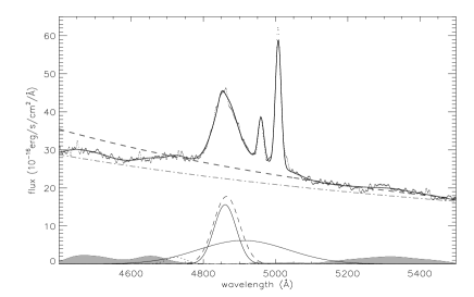
Figure 1: Effects of the broad He ii line on the line profile of the H$\beta$. The observed spectrum is shown in thin dotted line, the best fitted result is shown in the thick solid line, the dot-dashed line and the thick dashed line under the spectrum are for the power law components with and without the considerations of the broad He ii line. The shadow area near the bottom shows the weak Fe ii components, the dashed line near the bottom shows the gaussian broad component for the observed broad H$\beta$ without the consideration of the broad He ii, the two solid lines near the bottom show the two gaussian broad components for the observed broad H$\beta$ with the consideration of the broad He ii, the dotted line near the bottom shows the broad He ii component.

In Kaspi et al. (2000), Peterson et al. (2004) and in Zhang (2011b), the AGN continuum emission underneath the observed H$\beta$ is determined by the two continuum windows with the rest-wavelength from 4690Åto 4750Åand from 5115Åto 5175Å, without the considerations of the effects of the weak Fe ii and He ii lines. It is clear that the blue window used to determine the continuum is on the shoulder of the broad He ii line, which will lead to much steeper determined AGN continuum, and lead to much weak broad wings of the broad H$\beta$. Figure 1 shows the effects of the broad He ii line on the the determined AGN continuum, and then the effects on the line parameters of the H$\beta$. In the figure, the spectrum of PG 0052+251 observed on 14th, Nov. 1993 is shown, because of the more apparent He ii and optical Fe ii lines in the spectrum. The spectral properties are discussed twice as follows. On the one hand, the spectral lines are fitted within the wavelength range from 4690Åto 5175Åwithout the consideration of the He ii line, as what have been done in the literature. On the other hand, the spectral lines are fitted within the wavelength range from 4400Åto 5500Åwith the consideration of the He ii line and the weak optical Fe ii lines. It is clear that there are strong effects of the He ii line on the determined AGN continuum (the dashed and the dot-dashed lines in the Figure 1).

Then, the line profile of the broad H$\beta$ is roughly checked. More detailed discussions about the fitting procedure for the emission lines could be found in the following subsection. If the spectral lines are considered within the narrower wavelength range from 4690Åto 5175Å, the broad H$\beta$ can be well described by one broad gaussian function (the dashed line near the bottom in the Figure 1). However, the broad H$\beta$ can be well described by two broad gaussian functions ( the solid lines near the bottom in the Figure 1), if the spectral lines are considered within the wider wavelength range from 4400Åto 5500Å. Actually, the more recent optical Fe ii template discussed in the Kovacevic et al. (2010) has been included in our procedure, in order to clearly remove the probable effects of the optical Fe ii lines (the shadow areas near the bottom in the Figure 1). Based on the results in the Figure 1, we can find that the Fe ii lines are much weak and have few effects on our results about the line parameters of the broad H$\beta$.

It is clear that there are apparent and strong effects of the He ii line on the final results, especially on the AGN continuum and on the wings of the broad H$\beta$. Thus, the effects of the He ii line should be well considered. And therefore, in the following procedure to fit the spectral lines around the H$\beta$, the wider wavelength range from 4400Åto 5500Åis accepted, rather than the narrower wavelength range from 4690Åto 5175Å.

2.2 Line Parameters of the broad H$\beta$ and the broad H$\alpha$

In the manuscript, in order to obtain more reliable line parameters, the lines around the H$\alpha$ (the broad and the narrow H$\alpha$ and the [N ii]$\lambda 6548,6583$Ådoublet) and around the H$\beta$ (the broad and the narrow H$\beta$, the broad He ii line, the [O iii]$\lambda 4959,5007$Ådoublet and the optical Fe ii line) are fitted simultaneously within the wavelength ranges from 4400Åto 5500Åfor the lines around the H$\beta$ and the ranges from 6300Åto 6900Åfor the lines around the H$\alpha$.

In the manuscript, two different models are considered to describe the observed broad balmer lines: the model with two broad gaussian functions applied for each observed broad balmer line, and the other model with one broad gaussian function applied for each observed broad balmer line. Besides the two models for the broad balmer lines, the narrow lines are described by narrow gaussian functions with similar line profiles, i.e., they have the same emission line redshifts, the same line width. And moreover, the [O iii] ([N ii]) doublet has the fixed theoretical intensity ratio. Furthermore, one broad gaussian function is applied for the He ii line. Then, two power law functions are applied for the continuum under the H$\beta$ and the continuum under the H$\alpha$ ($f_{\lambda}\propto\lambda^{\alpha}$).

Moreover, when two broad gaussian functions are applied for each observed broad balmer line, the following restrictions are set:

$$\begin{split}\frac{\sigma(H\alpha_{1})}{\sigma(H\alpha_{2})}&=\frac{\sigma(H\beta_{1})}{\sigma(H\beta_{2})}\\ z(H\beta_{1})&=z(H\alpha_{1})\\ z(H\beta_{2})&=z(H\alpha_{2})\end{split}$$ (2)

where $\sigma$ and $z$ mean the broad line width (the second moment as discussed in Peterson et al. 2004) and the broad emission line redshift of the corresponding broad component, the suffixes ’1’ and ’2’ represent the broad components from the corresponding broad line regions (’1’ for the inner broad component and ’2’ for the intermediate broad component). The restrictions can be reasonably accepted under the following considerations.

If the two broad components were physically true for the broad H$\alpha$ and the broad H$\beta$, the result could be expected under the virialization assumption that

$$\frac{R_{BLR}(H\alpha_{1})\times\sigma(H\alpha_{1})}{R_{BLR}(H\alpha_{2})\times\sigma(H\alpha_{2})}=\frac{R_{BLR}(H\beta_{1})\times\sigma(H\beta_{1})}{R_{BLR}(H\beta_{2})\times\sigma(H\beta_{2})}$$ (3)

where $R_{BLR}$ means the distance between the broad line region and the central black hole. Once the results $R_{BLR}(H\alpha)\sim R_{BLR}(H\beta)$ are accepted, we can find the restriction for the line width ratio in the equation (2). And moreover, once we accepted that the inner (intermediate) broad components of the H$\alpha$ and the H$\beta$ from the same physical emission region, the restriction on the broad line redshift in equation (2) can be naturally accepted.

According to the models above and the corresponding restrictions, the spectral lines can be well fitted through the Levenberg-Marquardt method. Then, the results are firstly checked under the model with one broad gaussian function applied for each observed broad balmer line. Here, we do not show the best fitted results for all the 53 observed spectra, but two simple examples with the maximum and the minimum line widths of the broad H$\beta$ in the Figure 2. The basic correlations of the line parameters of the broad H$\alpha$ and the broad H$\beta$ are checked and shown in Figure 3. It is clear that there is no clear broad line width correlation: the spearman correlation coefficient is 0.14 with $P_{null}=30\%$, and no clear broad line flux correlation: the coefficient is 0.29 with $P_{null}\sim 3\%$. If the broad H$\alpha$ and the broad H$\beta$ are from the unique region, strong broad line flux and broad line width correlations should be expected. The much weak correlations shown in the Figure 3 indicate single broad component applied for each broad balmer line is not so reasonable, and further considerations should be checked.

Then, the model with two broad components applied for each observed broad balmer line is considered, with the restrictions in the equation (2). And moreover, by the following three steps, the model can be checked and further confirmed. The broad line parameters of the broad balmer lines are firstly checked under the model. Then, the F-test technique is applied to check which model is preferred for the broad balmer lines. Finally, the time-lagged correlations are checked.

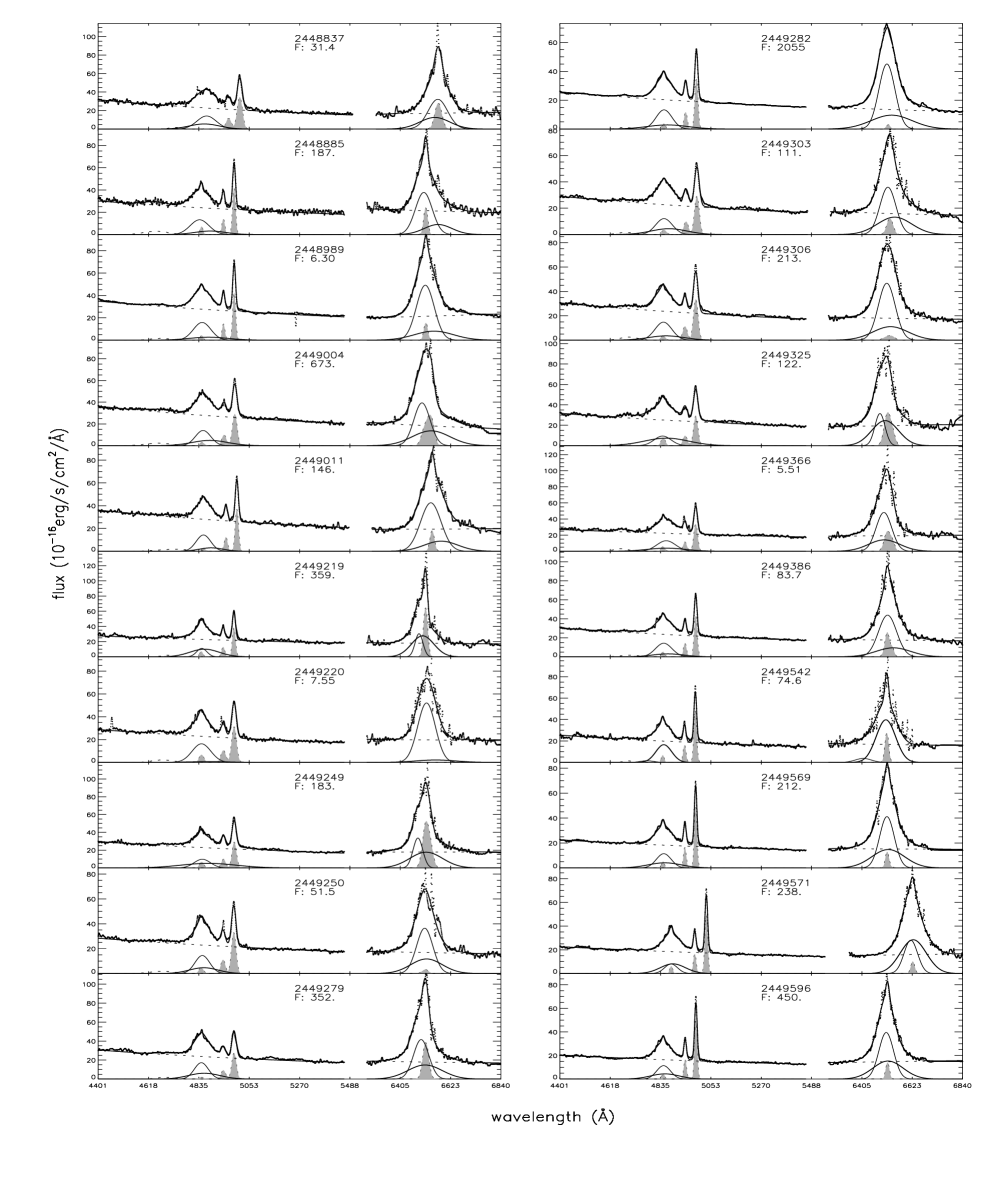
Figure 4: Best fitted results for the lines around the H$\beta$ and around the H$\alpha$ under the model with two broad components applied for each observed broad balmer line. The dotted lines are for the observed spectra, the thick solid lines are for the best fitted results, the AGN continuum is shown in the dotted line under the spectrum. The thick and the thin solid lines near the bottom represent the two broad components for each observed broad balmer line, the shadow areas near the bottom show the narrow lines, the dotted line near the bottom shows the He ii line. In each panel, the information of the MJD (seven characters) and the F value (starting with F:) calculated by the equation (6) are marked.

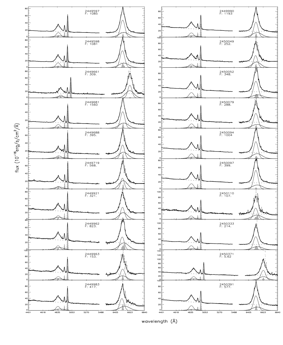
Figure 4: –continued.

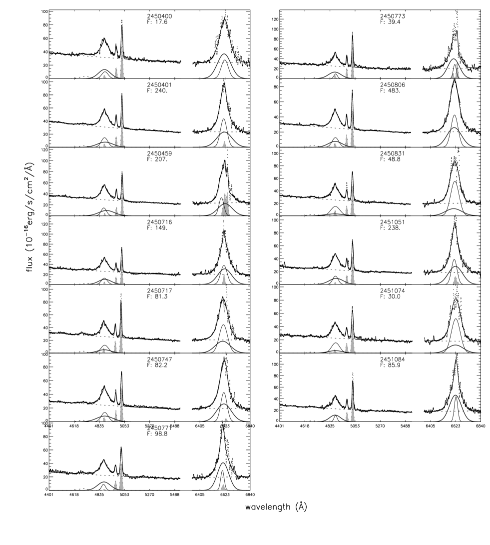
Figure 4: –continued.

The best fitted results for the spectral lines are shown in the Figure 4 under the model with two broad components applied for each observed broad balmer line. The measured line parameters are listed in the Table 1. Then, we check the correlations of the line parameters of the broad components of the balmer lines in the Figure 5. The corresponding correlations of the line parameters are apparent and strong (coefficient not less than 0.7 with $P_{null}$ less than $10^{-8}$, the corresponding coefficients and $P_{null}$ are marked in each panel of the figure),

$$\begin{split}\sigma(H\alpha_{1})&=0.95\times\sigma(H\beta_{1})\\ flux(H\alpha_{1})&=3.1\times flux(H\beta_{1})\\ \sigma(H\alpha_{2})&=0.93\times\sigma(H\beta_{2})\\ flux(H\alpha_{2})&=3.1\times flux(H\beta_{2})\end{split}$$ (4)

It is clear that the broad line width ratios and the broad line flux ratios for the inner/intermediate broad components are more reasonable.

Moreover, the properties about the relative shifted velocities of the two broad components are checked and shown as the open circles in the Figure 6. It is clear that the time dependent relative shift velocities are strongly linear decreasing (the coefficient is 0.61 with $P_{null}\sim 10^{-6}$), and the best fitted result (the solid line in the figure) can be written as,

$$\frac{W_{0}(1)-W_{0}(2)}{\rm km/s}\propto(-0.76\pm 0.04)\times(Julian-2448837)$$ (5)

Furthermore, the Figure 6 shows the properties of the relative shift velocities of the intermediate broad component relative to the narrow [O iii]$\lambda 5007$Å(solid circles in the figure). We can find that the intermediate broad components have tiny relative shift velocities to the narrow [O iii]. The time dependent rather than one randomly distributed relative shift velocities between the inner broad and the intermediate broad components strongly indicate the two components have physical meanings: one line region having no radial components and the other component having apparent radial moving contributions. Here, we should note the inner BLR including different contributions from different components DOES NOT have the similar meaning as the multiple BLRs. in the manuscript and in the literature, we accept and define that the inner BLR and the intermediate BLR mean they are two physical separated line emission regions with apparent physical space between the two regions. In other words, the observed complicated spectral broad lines do not indicate there are two or multiple BLRs, because the different line components were perhaps included in the same line region. Meanwhile, the current quality of the spectra can not provide further information to discuss whether the radial components are from the other line region which has apparent physical space from the inner BLR and/or the intermediate BLR. Thus, no further discussions about the radial motions are shown in the manuscript.

Then, the F-test technique is applied to determine which model is preferred for the observed broad balmer lines. Based on the best fitted results by the two models above, the F values firstly are calculated as

$$F=\frac{(SSE_{1}-SSE_{2})/(DoF_{1}-DoF_{2})}{SSE_{2}/(DoF_{2})}$$ (6)

where $SSE$ represents the sum of squared residual for one model, the suffix ’1’ is for the model with one broad component applied for each observed broad balmer line, and the suffix ’2’ is for the model with two broad components applied for each observed broad balmer line, $DoF$ represents the degree of freedom for one model. Through the comparison between the calculated value $F$ by the equation (6) and the F-value estimated by the F-distribution with the numerator degrees of freedom of $DoF_{1}-DoF_{2}$ and the denominator degrees of freedom of $DoF_{2}$, we can conclude our preferred model. Based on the selected wavelength range for the lines around the H$\alpha$ and around the H$\beta$ and the model parameters, the values of the degrees of freedom for the two models are: $DoF_{1}=1829$, $DoF_{2}=1826$. It is clear that the F-value by the F-distribution with $p=0.05$ is 2.6 (the IDL function $f\_cvf(0.05,3,DoF_{2}-1)$) based on the numerator and denominator degrees of freedom. However, the calculated values $F$ listed in the Figure 4 by the equation (6) are much larger than 2.6, which strongly indicates that it is more preferred to describe each observed broad balmer line by two broad components.

Furthermore, the time-lagged correlations are checked for the two broad components. If the inner and the intermediate broad components were physically true and from two independent line regions, there should be much different time lags between the variabilities of the AGN continuum and the two broad components. And then, based on the time-lagged results, we can confirm whether the model dependent line parameters are physically reliable or only the mathematical model results. Before proceeding further, one point we should note. Because of the effects of the He ii lines and the narrow lines around the H$\alpha$, it should be not so appropriate to directly use the scaled light curves of the H$\alpha$ and the H$\beta$ shown in the Kaspi et al. (2000), as what we have done in Paper I. Therefore, the light curves of the two broad components of the H$\beta$ (the H$\alpha$) are determined with the assumption that the [O iii]$\lambda 5007$Åflux is constant,

$$flux=flux(obs)\times\frac{710\times 10^{-16}{\rm erg/s/cm^{2}}}{flux([OIII]\lambda 5007\AA)}$$ (7)

where $710\times 10^{-16}{\rm erg/s/cm^{2}}$ is the mean flux of the [O iii]$\lambda 5007$Å, $flux(obs)$ is the line flux for the corresponding broad component directly measured through the observed spectrum, $flux$ means the corrected line flux. It is clear that there is no time-dependent trend for the [O iii], and the rms variation about the mean is around 10%, which indicates the flux normalization to the [O iii] flux is necessary. Moreover, we can find that the center wavelengths of the [O iii]$\lambda 5007$Åhave tiny shifts, which is perhaps due to the large dispersions and spectral resolutions of the original spectra of PG 0052+251 (Kaspi et al. 2000). Meanwhile, the center wavelength shifts of the [O iii] have few effects on our final results about the broad line parameter correlations. Thus, there are no further discussions about the shifts in the manuscript.

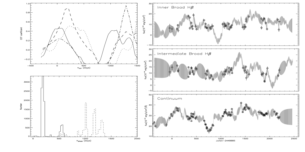
Figure 7: The ICCF and SPEAR results for the inner and the intermediate broad components of the H$\beta$ of PG 0052+251. Top left panel shows the ICCF results for the inner broad H$\beta$ (dotted line for the result through the observational light curves, dashed line for the result through the light curves determined by the random walk model) and the intermediate broad H$\beta$ (solid line for the result through the observational light curves, dot-dashed line for the result through the light curves determined by the random walk model), and bottom left panel shows the distributions of the time lags determined by the SPEAR method (thin solid line for H$\beta_{1}$ and thick dotted line for H$\beta_{2}$). The right panels from top to bottom shows the observational light curves (open circles) of the inner broad H$\beta$, the intermediate broad H$\beta$ and the continuum emission, and the corresponding best descriptions for the observational light curves by the damped random walk model for AGN variability.

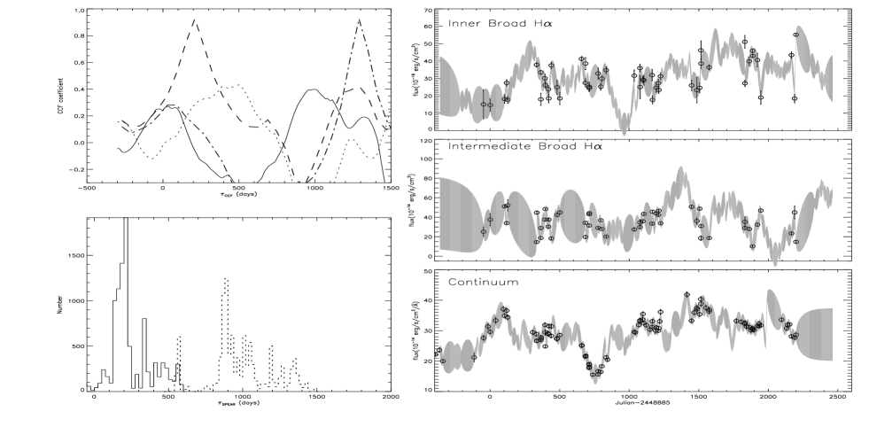
Figure 8: The ICCF and SPEAR results for the H$\alpha$, symbols and lines have the same meanings as those in the Figure 7, but for the H$\alpha$.

Once the observational light curves of the broad components are determined, the commonly accepted ICCF technique (Interpolated Cross Correlation Function, Gaskell & Peterson 1987, Koratkar & Gaskell 1989, Koptelova et al. 2006, Peterson 1993) and the more recent SPEAR technique (Stochastic Process Estimation for AGN Reverberation based on the damped random walk model for AGN variability, Kelly et al. 2009, Kozlowski et al. 2010, MacLeod et al. 2010, Zu et al. 2011) are applied to check the time lags between the variabilities of the continuum and the inner/intermediate broad components. Here, the light curve of the continuum is the one collected from Kaspi et al. (2000). Moreover, when the commonly used ICCF method is applied, the direct interpolating method is not only applied to the measured observational light curves (the open circles in the right panels of Figure 7 and Figure 8) of the broad components and the continuum emission, but also applied to the best descriptions of the light curves determined by the damped random walk method (the shadow areas in the right panels of Figure 7 and Figure 8), in order to reduce the effects of the large time gaps of the observational light curves. Moreover, the two different method (ICCF and SPEAR) should lead to more reliable results, if there were similar ICCF and SPEAR results.

The time-lagged correlations are shown in the Figure 7 for the broad components of the H$\beta$ and in the Figure 8 for the broad components of the H$\alpha$. It is clear that there are apparent ans different time lags between the broad components and the AGN continuum based on the ICCF and SPEAR results,

$$\begin{split}R_{BLR}(H\beta_{1},ICCF)&\simeq R_{BLR}(H\alpha_{1},ICCF)\\ &\sim 270\pm 80\hskip 7.11317pt{\rm light-days}\\ R_{BLR}(H\beta_{1},SPEAR)&\simeq R_{BLR}(H\alpha_{1},SPEAR)\\ &\sim 211\pm 50\hskip 7.11317pt{\rm light-days}\\ R_{BLR}(H\beta_{2},ICCF)&\simeq R_{BLR}(H\alpha_{2},ICCF)\\ &\sim 1200\pm 300\hskip 7.11317pt{\rm light-days}\\ R_{BLR}(H\beta_{2},SPEAR)&\simeq R_{BLR}(H\alpha_{2},SPEAR)\\ &\sim 1056\pm 160\hskip 7.11317pt{\rm light-days}\\ \end{split}$$ (8)

where the uncertainties with $3\sigma$ confidence levels of the time lags are determined by the bootstrap method as what we have done in Paper I, and the ICCF results are the mean values based on the observational light curves and the light curves determined through the random walk method. The results strongly support that the two model dependent broad components are both mathematically and physically true, and have much different structures, and it is more preferred to describe the observed broad balmer line by two broad components for PG 0052+251.

2.3 On the Correlation between the Line Width and the Line Flux

Now, based on the reliable measured line parameters and the corresponding uncertainties, the correlations of the broad line parameters of the two broad components of the balmer lines can be checked. The linear correlation coefficients are about -0.63 with $P_{null}\sim 9\times 10^{-7}$, 0.72 with $P_{null}\sim 5\times 10^{-9}$, -0.48 with $P_{null}\sim 4\times 10^{-4}$ and 0.69 with $P_{null}\sim 9\times 10^{-8}$ for the correlations between the line width and the line flux for the inner broad H$\alpha$, for the intermediate broad H$\alpha$, for the inner broad H$\beta$ and for the intermediate broad H$\beta$ respectively. The strong correlations are shown in Figure 9. It is clear that there are much different properties for the inner and the intermediate broad components of PG 0052+251: one clear positive correlation for the intermediate broad component, but one clear negative correlation for the inner broad component. The best fitted results for the correlations with the considerations about the uncertainties in both the coordinates can be written as,

$$\begin{split}\log(\frac{flux(H\alpha_{1})}{10^{-16}{\rm ergs/s/cm^{2}}})&=(7.89\pm 0.21)\\ &-(1.27\pm 0.06)\times\log(\frac{\sigma(H\alpha_{1})}{\rm km/s})\\ \log(\frac{flux(H\alpha_{2})}{10^{-16}{\rm ergs/s/cm^{2}}})&=(-2.16\pm 0.33)\\ &+(1.81\pm 0.11)\times\log(\frac{\sigma(H\alpha_{2})}{\rm km/s})\\ \log(\frac{flux(H\beta_{1})}{10^{-16}{\rm ergs/s/cm^{2}}})&=(8.69\pm 0.39)\\ &-(1.65\pm 0.12)\times\log(\frac{\sigma(H\beta_{1})}{\rm km/s})\\ \log(\frac{flux(H\beta_{2})}{10^{-16}{\rm ergs/s/cm^{2}}})&=(-2.85\pm 0.41)\\ &+(1.85\pm 0.13)\times\log(\frac{\sigma(H\beta_{2})}{\rm km/s})\end{split}$$ (9)

Meanwhile, the corresponding 99.95% confidence bands for the best fitted results above are also shown in Figure  9.

Before the end of the subsection, one point we should mote. Based on the fitted results shown in the Figure 4 and the listed line parameters in the Table 1, we can find that there are five spectra of which the narrow H$\alpha$ (and/or [N ii]$\lambda 6583\AA$) are much stronger, while the narrow H$\beta$ are much weaker: JD-2448837, JD-2449219, JD-2449249, JD-2449279 and JD-2450459. We do not know the clear reason why the narrow balmer lines are much different from the lines in the other spectra. However, we can find that the results have few effects on our final results about the broad line parameters correlations, because no different re-calculated broad line parameters correlations can be found without the considerations of the five spectra with the different narrow lines. Without the considerations of the five cases, the corresponding correlation coefficients are about -0.62 with $P_{null}\sim 6\times 10^{-6}$, 0.74 with $P_{null}\sim 3\times 10^{-9}$, -0.49 with $P_{null}\sim 7\times 10^{-3}$ and 0.72 with $P_{null}\sim 2\times 10^{-8}$ for the correlations between the broad line width and the broad line flux for the inner broad H$\alpha$, for the intermediate broad H$\alpha$, for the inner broad H$\beta$ and for the intermediate broad H$\beta$ respectively. Therefore, no apparent effects of the narrow lines in the several special cases can be found for our final results. Thus, there are no further discussions about the cases with special narrow lines in the manuscript.

As we commonly know that the properties of the broad line flux can be used to trace the distance between the broad line clouds and the central black hole, and the properties of the line width can be used to trace the kepler velocities of the broad line clouds. The different correlations between the line width and the line flux for the inner and the intermediate broad components strongly indicate there are much different properties of the two broad line regions of PG 0052+251.

3 Discussions and Conclusions

It is clear that based on the widely accepted Virialization assumption for the broad line AGN, the negative correlation between the line width and the line flux can be expected for individual object. Such negative correlation has been found and confirmed for several mapped objects, such as NGC5548 (Bentz et al. 2006, Denney et al. 2010, Peterson et al. 2004, Zhang 2011a) and some other mapped objects discussed in Peterson et al. (2004). Then based on the empirical relation to estimate the size of the BLR $R_{BLR}\propto L^{\alpha}$ (Bentz et al. 2006, 2009, Denney et al. 2010, Kaspi et al. 2005, Greene et al. 2010, Wang & Zhang 2003), one strongly negative correlation between the broad line flux and the broad line width can be expected for individual object. Meanwhile, the common viewpoint about gravity dominated BLR can be used to naturally explain the negative correlation (Kollatschny & Zetzl1 2011, Krause et al. 2011, Netzer & Marziani 2010, Peterson & Wandel 1999, and references therein).

Moreover, we should note that if the common value $\alpha\sim 0.5$ was accepted for the empirical relation to estimate the BLR size of AGN, we should expect the slope of the correlation for the inner broad component is about $-4$, which is smaller than the reported slope, $\sim-1.5$ shown in Figure 9 for PG 0052+251. The difference can be well and naturally explained by the following reason: the shape of the continuum changes as AGNs vary, i.e., variability amplitudes are different for UV and optical bands. And moreover, UV flux rather than optical flux is a better measure for ionizing flux which is one much better indicator for the size of BLR. So that, the different variability amplitudes in UV and optical bands lead to some different slope from $-4$ for the correlations of the inner broad components of PG 0052+251, and smaller variability amplitudes in optical bands lead to the slope larger than $-4$.

Besides the negative correlation for the inner broad H$\alpha$, there is one clear positive correlation between the line width and the line flux for the intermediate broad components of PG 0052+251, which is against the virialization assumption. However, we (Zhang 2013a) have recently reported that there is one positive correlation between the line width and the line flux of the broad double-peaked H$\alpha$ of the well-known mapped object 3C390.3. Furthermore, we have discussed that the positive correlation of broad line parameters could be used as one indicator for the accretion disk origination of the broad lines. So that, if the accretion disk origination was accepted for the intermediate broad components of PG 0052+251, the positive correlation could be naturally explained, as we have explained the positive correlation for the double-peaked emitter of 3C390.3.

Although there are different dependent modes of the size of BLR on the line flux for the two components, the correlation between the measured size of the BLR (not the line flux) and the line width can be checked under the virialization assumption: similar black hole masses determined by the properties of the inner BLR and the intermediate BLR

$$\begin{split}\frac{R_{BLR}(H\alpha_{1})\times\sigma^{2}(H\alpha_{1})}{R_{BLR}(H\alpha_{2})\times\sigma^{2}(H\alpha_{2})}\sim\frac{\frac{226}{{\rm light-days}}\times(\frac{3100}{{\rm km/s}})^{2}}{\frac{1090}{{\rm light-days}}\times(\frac{1400}{{\rm km/s}})^{2}}=1.01\\ \end{split}$$ (10)

where $\sigma(H\alpha_{1})\sim 3100{\rm km/s}$ and $\sigma(H\alpha_{2})\sim 1400{\rm km/s}$ are the mean line widths of the inner broad and the intermediate broad components of the H$\alpha$, and $R_{BLR}$ is the weighted mean value from the ICCF and SPEAR results (Equation (8)). Similar result can be confirmed for the two broad components of the H$\beta$. The results indicate the measured time lags for the inner/intermediate broad components are reliable, and the two model-calculated components are not fake.

Before the end of the manuscript, there are two points we should note. On the one hand, the main objective of the manuscript is to provide further evidence for the intermediate BLR of PG 0052+251. The much different and reliable correlations for the two components in the Figure 9 provide enough evidence to support our objective. Therefore, no further discussions are shown for the detailed structure information on the two broad components. The apparent time-dependent shifted velocities of the inner broad component (Figure 6) indicates probable radial contributions for the component. The positive correlation provides the possibility for the accretion disk origination of the intermediate broad components. So far only two individual AGNs, 3C390.3 in our previous paper and PG 0052+251 in the manuscript, have shown the positive correlation between the line width and the line flux. Meanwhile, the accretion disk origination for the double-peaked broad lines have been widely accepted for the 3C390.3. Therefore, we naturally presume but not confirm that the intermediate broad balmer lines of PG 0052 have the similar characters as the lines of 3C390.3. Surely, more efforts should be done to give the final confirmed conclusions about the structures of the two components, which is beyond the scope of the manuscript. On the other hand, more reasonable continuum windows are selected to determine the AGN continuum especially under the H$\beta$ in the manuscript, which leads to some different BLR size based on the H$\beta$ variabilities. If the contributions of the narrow lines are subtracted, the measured size of the BLR is around $R\sim 200$ light-days based on the H$\beta$ variabilities, similar with the values determined by the H$\alpha$ variabilities. Therefore, the position of PG 0052+251 is reasonable in the plane of $(\frac{\sigma(H\beta)}{\sigma(H\alpha)})^{2}$ versus $\frac{R_{BLR,H\alpha}}{R_{BLR,H\beta}}$. The selected narrower wavelength range to determine the continuum lead the inner broad H$\beta$ being much weakened. Yet, in other ways, it is effective to select the objects with probable intermediate BLR through the properties of objects in the plane of $(\frac{\sigma(H\beta)}{\sigma(H\alpha)})^{2}$ versus $\frac{R_{BLR,H\alpha}}{R_{BLR,H\beta}}$.

Our final main conclusions are as follows.

• The observed broad balmer lines are being fitted by two models. If the model with only one simple broad component was applied for each observed broad balmer line, the corresponding broad line parameters correlations between the broad H$\alpha$ and the broad H$\beta$ are much weak (Figure 3). However, Under model with two broad components applied for each observed broad balmer line, the broad line width and the broad line flux correlations are much strong and more reasonable for the corresponding broad components of the H$\alpha$ and the H$\beta$ (Figure 5). Moreover, the F-test technique has been applied to check the two models, and indicates two broad components for the broad balmer line (Figure 4) are preferred. Then, the time-lagged correlations have been checked for the two components (Figure 7 and Figure 8). The much different time lags between the two broad components and the continuum ensure that the two components are not mathematical model dependent components but have physical meanings for different geometric structures.

• Based on the measured line parameters, one positive correlation between the line width and the line flux can be found for the intermediate broad component, but one negative correlation can be found for the inner broad component, of the balmer lines of PG 0052+251. The different correlations strongly support the intermediate BLR of PG 0052+251, and clearly indicate the inner BLR and the intermediate BLR have much different dynamic/geometric structures.

Table 1: Line Parameters of PG 0052+251

JD	Inner Broad			Intermediate Broad			[O iii]			’ ’
	$W_{0}$	$\sigma$	flux	$W_{0}$	$\sigma$	flux	$W_{0}$	$\sigma$	flux	flux(H$\beta_{N}$)	flux(H$\alpha_{N}$)	flux([N ii])
48837	4858.9$\pm$5.0	3967$\pm$469	8.81$\pm$4.88	4868.6$\pm$1.7	2568$\pm$234	14.68$\pm$4.74	5012.0$\pm$0.3	660$\pm$17	9.53$\pm$0.28	0.13$\pm$0.40	10.05$\pm$1.17
	6554.4$\pm$6.6	2965$\pm$349	20.29$\pm$11.21	6567.5$\pm$2.3	1920$\pm$234	33.86$\pm$6.41
48885	4900.7$\pm$18.2	4249$\pm$640	5.46$\pm$2.41	4853.4$\pm$1.7	2591$\pm$177	13.95$\pm$2.06	5007.6$\pm$0.2	389$\pm$13	6.74$\pm$0.24	1.13$\pm$0.25	5.07$\pm$0.58
	6619.1$\pm$24.1	2828$\pm$640	13.98$\pm$3.25	6555.3$\pm$1.3	1724$\pm$95.7	35.75$\pm$5.73
48989	4893.5$\pm$5.5	5253$\pm$365	5.51$\pm$0.74	4864.7$\pm$1.4	2406$\pm$107	15.45$\pm$0.78	5008.0$\pm$0.2	383$\pm$14	6.81$\pm$0.24	0.67$\pm$0.27	3.22$\pm$0.62
	6600.8$\pm$7.2	3972$\pm$227	17.48$\pm$2.28	6561.9$\pm$1.9	1819$\pm$107	49.05$\pm$1.06
49004	4899.3$\pm$3.2	4925$\pm$338	9.71$\pm$0.88	4869.0$\pm$1.7	2117$\pm$142	12.03$\pm$0.77	5010.7$\pm$0.4	611$\pm$22	7.45$\pm$0.29	0.69$\pm$0.46	4.14$\pm$0.95	7.73$\pm$1.04
	6587.8$\pm$3.6	3852$\pm$115	28.82$\pm$1.87	6547.1$\pm$2.3	1656$\pm$142	35.74$\pm$1.04
49011	4895.3$\pm$11.1	3187$\pm$328	3.85$\pm$1.31	4861.8$\pm$1.9	1955$\pm$153	11.34$\pm$1.49	5008.2$\pm$0.2	424$\pm$16	6.53$\pm$0.24	0.49$\pm$0.32	4.14$\pm$0.61
	6603.8$\pm$16.1	3363$\pm$328	16.35$\pm$1.77	6558.6$\pm$1.4	2062$\pm$90	48.13$\pm$5.21
49219	4875.3$\pm$1.5	4012$\pm$219	16.38$\pm$0.76	4863.2$\pm$1.4	1398$\pm$136	6.286$\pm$0.61	5006.9$\pm$0.2	407$\pm$12	6.52$\pm$0.24	1.18$\pm$0.34	14.31$\pm$0.93
	6550.1$\pm$1.2	2297$\pm$48	34.81$\pm$1.19	6533.8$\pm$1.8	801$\pm$136	13.35$\pm$0.81
49220	4892.2$\pm$17.1	5728$\pm$1002	1.53$\pm$0.58	4861.8$\pm$1.3	2570$\pm$110	17.01$\pm$0.71	5007.6$\pm$0.3	629$\pm$18	8.18$\pm$0.24	1.72$\pm$0.38
	6608.3$\pm$23.2	4027$\pm$1002	4.63$\pm$0.79	6567.3$\pm$0.7	1806$\pm$38	51.64$\pm$1.81
49249	4893.0$\pm$2.3	7634$\pm$388	15.89$\pm$0.82	4865.5$\pm$1.8	2252$\pm$159	8.91$\pm$0.54	5008.3$\pm$0.3	569$\pm$19	6.86$\pm$0.26	1.54$\pm$0.34	13.45$\pm$1.07	6.71$\pm$0.62
	6565.7$\pm$1.7	3341$\pm$80	32.45$\pm$1.14	6528.9$\pm$2.4	985$\pm$159	18.18$\pm$0.72
49250	4871.8$\pm$2.6	3916$\pm$338	7.39$\pm$1.43	4865.6$\pm$1.2	2022$\pm$130	11.88$\pm$1.38	5006.1$\pm$0.3	594$\pm$18	8.15$\pm$0.25	1.13$\pm$0.41	1.01$\pm$0.91
	6567.5$\pm$3.1	3223$\pm$237	20.71$\pm$3.98	6559.1$\pm$1.7	1664$\pm$130	33.28$\pm$1.86
49279	4874.1$\pm$2.2	4327$\pm$286	10.79$\pm$0.95	4861.2$\pm$1.1	1930$\pm$109	13.51$\pm$0.92	5007.7$\pm$0.3	584$\pm$19	6.73$\pm$0.24	0.43$\pm$0.47	12.22$\pm$1.05
	6560.6$\pm$2.4	3512$\pm$139	28.55$\pm$2.25	6543.3$\pm$1.5	1566$\pm$109	35.73$\pm$1.25
49282	4881.5$\pm$2.3	5581$\pm$288	6.41$\pm$0.41	4865.9$\pm$1.2	2198$\pm$92	11.85$\pm$0.46	5010.4$\pm$0.2	409$\pm$13	5.96$\pm$0.19	0.63$\pm$0.23	0.62$\pm$0.53
	6582.7$\pm$2.6	4183$\pm$143	22.01$\pm$1.29	6561.6$\pm$1.6	1648$\pm$91	40.74$\pm$0.62
49303	4884.6$\pm$2.9	4903$\pm$316	8.85$\pm$0.77	4862.6$\pm$1.5	2292$\pm$132	11.25$\pm$0.71	5008.6$\pm$0.3	615$\pm$20	7.49$\pm$0.26	0.85$\pm$0.37	4.11$\pm$0.91
	6585.9$\pm$3.3	3485$\pm$113	25.24$\pm$2.01	6556.1$\pm$2.1	1629$\pm$132	32.10$\pm$0.96
49306	4875.7$\pm$3.3	4845$\pm$370	6.87$\pm$0.96	4863.1$\pm$1.3	2321$\pm$126	13.93$\pm$0.95	5007.6$\pm$0.3	595$\pm$18	8.37$\pm$0.26	0.85$\pm$0.39	0.63$\pm$0.96	0.92$\pm$0.91
	6577.9$\pm$3.8	3611$\pm$208	21.88$\pm$2.99	6561.0$\pm$1.8	1730$\pm$126	44.34$\pm$1.28
49325	4876.6$\pm$2.2	6137$\pm$328	18.36$\pm$1.25	4859.4$\pm$1.9	2324$\pm$202	8.91$\pm$0.92	5007.7$\pm$0.3	575$\pm$22	6.94$\pm$0.31	1.75$\pm$0.37	8.33$\pm$1.21	4.34$\pm$0.65
	6553.6$\pm$1.4	2726$\pm$75	36.73$\pm$1.91	6530.5$\pm$2.6	1032$\pm$202	17.81$\pm$1.24
49366	4876.6$\pm$2.6	5219$\pm$397	8.08$\pm$1.38	4875.6$\pm$1.5	2590$\pm$135	13.70$\pm$1.36	5007.3$\pm$0.2	499$\pm$16	7.03$\pm$0.25	1.16$\pm$0.28	5.67$\pm$0.89	3.69$\pm$0.74
	6549.6$\pm$2.4	3207$\pm$218	24.77$\pm$4.02	6548.2$\pm$2.0	1591$\pm$135	42.04$\pm$1.84
49386	4883.7$\pm$4.8	4328$\pm$330	5.42$\pm$1.02	4864.6$\pm$1.4	2269$\pm$115	13.17$\pm$1.01	5007.3$\pm$0.2	393$\pm$12	7.01$\pm$0.23	0.85$\pm$0.26	5.26$\pm$0.68	2.21$\pm$0.61
	6590.4$\pm$6.1	3533$\pm$219	18.31$\pm$3.43	6564.6$\pm$1.9	1852$\pm$115	44.54$\pm$1.36
49542	4864.7$\pm$1.4	2175$\pm$78	14.58$\pm$0.54	4789.8$\pm$8.5	1771$\pm$368	1.11$\pm$0.36	5005.6$\pm$0.1	370$\pm$11	7.42$\pm$0.22	1.01$\pm$0.22	5.53$\pm$0.48
	6557.0$\pm$1.5	1980$\pm$51	43.17$\pm$1.24	6456.1$\pm$11.1	1612$\pm$368	3.27$\pm$0.49
49569	4869.0$\pm$1.8	4559$\pm$251	7.59$\pm$0.65	4864.7$\pm$1.2	2040$\pm$97	9.47$\pm$0.65	5007.0$\pm$0.1	347$\pm$9	7.08$\pm$0.22	0.74$\pm$0.22	2.44$\pm$0.65	0.12$\pm$0.54
	6567.6$\pm$1.7	3369$\pm$141	27.27$\pm$2.32	6561.8$\pm$1.6	1508$\pm$97	34.04$\pm$0.87
49571	4869.1$\pm$1.5	3193$\pm$160	10.55$\pm$0.97	4861.5$\pm$1.3	1656$\pm$136	5.39$\pm$0.94	5007.7$\pm$0.1	346$\pm$9	7.12$\pm$0.21	0.88$\pm$0.21	1.91$\pm$0.57
	6566.0$\pm$1.3	2476$\pm$81	38.67$\pm$3.44	6555.8$\pm$1.8	1284$\pm$136	19.78$\pm$1.27

Notice: The first column gives the observational dates (JD-2400000), the second to forth columns show the line parameters of the inner broad component: center wavelength $W_{0}$ in unit of $\AA$, line width $\sigma$ in unit of ${\rm km/s}$ and line flux in unit of $10^{-14}{\rm erg/s/cm^{2}}$, the fifth to seventh columns show the line parameters of the intermediate broad component, the eighth to tenth columns show the line parameters of the narrow [O iii], the last three columns show the line fluxes (in unit of $10^{-14}{\rm erg/s/cm^{2}}$) of the narrow H$\beta$, narrow H$\alpha$ and [N ii]$\lambda 6583\AA$. Because the narrow lines have the same line redshift and the same line width (${\rm km/s}$), thus we do not list the center wavelengths and the line widths of the narrow H$\beta$, the narrow H$\alpha$ and the [N ii] line in the table. The first line of every two rows lists the parameters for the two components of the H$\beta$ (second to seventh columns), and the second line lists the parameters for the H$\alpha$ (second to seventh columns).

Table 1: continued

JD	Inner Broad			Intermediate Broad			[O iii]			’ ’
	$W_{0}$	$\sigma$	flux	$W_{0}$	$\sigma$	flux	$W_{0}$	$\sigma$	flux	flux(H$\beta_{N}$)	flux(H$\alpha_{N}$)	flux([N ii])
49596	4869.7$\pm$1.7	3929$\pm$221	7.02$\pm$0.76	4863.8$\pm$1.2	1903$\pm$95	8.78$\pm$0.75	5008.1$\pm$0.1	353$\pm$8	7.29$\pm$0.19	0.65$\pm$0.19	2.69$\pm$0.55
	6566.5$\pm$1.7	3093$\pm$141	25.95$\pm$2.74	6558.5$\pm$1.4	1498$\pm$95	32.46$\pm$1.01
49597	4877.4$\pm$1.9	4464$\pm$209	6.29$\pm$0.54	4865.5$\pm$1.3	2097$\pm$78	10.77$\pm$0.55	5009.4$\pm$0.1	361$\pm$8	6.83$\pm$0.18	0.81$\pm$0.19	1.81$\pm$0.54
	6577.9$\pm$2.1	3393$\pm$124	24.25$\pm$2.04	6561.8$\pm$1.3	1594$\pm$77	41.51$\pm$0.75
49598	4878.5$\pm$2.2	4476$\pm$209	6.43$\pm$0.54	4861.8$\pm$1.0	2105$\pm$75	11.62$\pm$0.55	5006.7$\pm$0.1	356$\pm$8	6.94$\pm$0.18	0.75$\pm$0.19	2.33$\pm$0.59	1.01$\pm$0.52
	6579.9$\pm$2.6	3450$\pm$119	23.97$\pm$1.94	6557.4$\pm$1.3	1622$\pm$75	43.37$\pm$0.75
49661	4868.5$\pm$1.3	3446$\pm$173	6.69$\pm$0.66	4870.1$\pm$1.2	1736$\pm$101	5.91$\pm$0.64	5013.0$\pm$0.1	351$\pm$8	6.93$\pm$0.17	0.67$\pm$0.16	0.39$\pm$0.57
	6565.0$\pm$1.2	2703$\pm$100	32.13$\pm$3.11	6567.1$\pm$1.4	1362$\pm$101	28.40$\pm$0.87
49681	4877.5$\pm$1.9	4561$\pm$215	5.38$\pm$0.41	4864.1$\pm$1.1	2102$\pm$87	7.85$\pm$0.41	5010.1$\pm$0.1	364$\pm$8	6.67$\pm$0.17	0.78$\pm$0.16	2.13$\pm$0.51
	6580.0$\pm$2.0	3357$\pm$108	23.83$\pm$1.71	6562.0$\pm$1.5	1547$\pm$87	34.75$\pm$0.56
49688	4883.9$\pm$2.0	5483$\pm$255	7.57$\pm$0.51	4873.8$\pm$1.6	2417$\pm$115	7.05$\pm$0.47	5009.5$\pm$0.1	318$\pm$7	6.86$\pm$0.19	0.98$\pm$0.14	2.04$\pm$0.46
	6574.1$\pm$1.5	3204$\pm$95	28.98$\pm$1.73	6560.5$\pm$2.2	1412$\pm$115	26.97$\pm$0.63
49719	4875.3$\pm$1.8	3949$\pm$212	8.19$\pm$0.52	4864.9$\pm$1.5	1771$\pm$119	4.73$\pm$0.48	5011.3$\pm$0.1	321$\pm$8	6.87$\pm$0.19	0.78$\pm$0.16	2.08$\pm$0.46
	6571.7$\pm$1.3	2855$\pm$77	33.72$\pm$1.89	6557.6$\pm$2.1	1280$\pm$119	19.48$\pm$0.64
49921	4870.8$\pm$1.9	4081$\pm$263	10.03$\pm$1.08	4863.6$\pm$1.4	1978$\pm$133	8.719$\pm$1.05	5008.4$\pm$0.1	314$\pm$9	6.96$\pm$0.23	0.77$\pm$0.22	0.94$\pm$0.51
	6568.8$\pm$1.8	2903$\pm$130	31.05$\pm$3.20	6559.1$\pm$1.9	1408$\pm$133	26.99$\pm$1.42
49962	4880.3$\pm$2.7	4182$\pm$327	9.91$\pm$0.79	4860.8$\pm$1.8	1856$\pm$139	8.21$\pm$0.73	5007.9$\pm$0.2	349$\pm$12	6.62$\pm$0.24	0.76$\pm$0.26	1.79$\pm$0.59	2.94$\pm$0.56
	6580.8$\pm$2.4	3349$\pm$97	33.65$\pm$2.03	6554.4$\pm$2.5	1487$\pm$139	27.91$\pm$0.98
49963	4862.9$\pm$2.4	4208$\pm$416	7.92$\pm$2.11	4864.8$\pm$1.5	2320$\pm$176	10.92$\pm$2.10	5007.1$\pm$0.2	341$\pm$11	6.79$\pm$0.23	0.89$\pm$0.24	2.84$\pm$0.58
	6559.3$\pm$2.4	2961$\pm$271	24.03$\pm$6.37	6561.9$\pm$2.1	1633$\pm$176	33.14$\pm$2.84
49983	4892.1$\pm$3.2	4272$\pm$280	8.38$\pm$0.61	4858.8$\pm$1.5	1871$\pm$113	10.24$\pm$0.57	5007.3$\pm$0.2	325$\pm$11	6.47$\pm$0.24	0.56$\pm$0.25	3.72$\pm$0.51
	6594.7$\pm$3.8	3468$\pm$91	26.81$\pm$1.65	6549.9$\pm$2.2	1519$\pm$113	32.76$\pm$0.77
49990	4875.9$\pm$2.6	4628$\pm$301	7.65$\pm$0.77	4862.7$\pm$1.4	2146$\pm$113	11.48$\pm$0.78	5009.0$\pm$0.2	370$\pm$13	6.47$\pm$0.23	0.71$\pm$0.26	2.39$\pm$0.71	0.01$\pm$0.59
	6580.0$\pm$2.8	3352$\pm$145	26.42$\pm$2.56	6562.3$\pm$1.9	1555$\pm$113	39.66$\pm$1.05
50049	4874.9$\pm$2.3	4666$\pm$298	9.72$\pm$1.06	4864.2$\pm$1.6	2240$\pm$132	10.19$\pm$1.04	5007.2$\pm$0.2	348$\pm$11	6.59$\pm$0.23	0.82$\pm$0.23	2.08$\pm$0.72	0.08$\pm$0.57
	6572.2$\pm$2.3	3001$\pm$136	29.72$\pm$3.05	6557.8$\pm$2.1	1441$\pm$132	31.16$\pm$1.40
50052	4884.3$\pm$4.1	4710$\pm$315	6.07$\pm$0.78	4863.5$\pm$1.2	2214$\pm$96	15.64$\pm$0.83	5008.3$\pm$0.2	407$\pm$13	7.84$\pm$0.26	0.75$\pm$0.31	2.29$\pm$0.75	2.44$\pm$0.73
	6590.2$\pm$5.2	3618$\pm$196	19.59$\pm$2.51	6562.1$\pm$1.7	1701$\pm$96	50.55$\pm$1.13
50079	4879.9$\pm$2.8	4642$\pm$296	6.93$\pm$0.74	4865.8$\pm$1.3	2118$\pm$98	12.33$\pm$0.77	5009.3$\pm$0.1	343$\pm$11	6.94$\pm$0.22	0.68$\pm$0.24	1.83$\pm$0.63	0.05$\pm$0.51
	6580.2$\pm$3.3	3606$\pm$180	24.17$\pm$2.50	6561.2$\pm$1.7	1645$\pm$98	43.01$\pm$1.04
50094	4881.0$\pm$2.5	4778$\pm$286	7.66$\pm$0.68	4865.7$\pm$1.3	2165$\pm$104	11.87$\pm$0.69	5009.8$\pm$0.2	405$\pm$13	6.76$\pm$0.23	0.79$\pm$0.26	1.54$\pm$0.69	0.44$\pm$0.60
	6582.3$\pm$2.7	3453$\pm$133	26.09$\pm$2.15	6561.7$\pm$1.8	1565$\pm$104	40.47$\pm$0.93
50097	4880.6$\pm$2.7	5178$\pm$292	6.67$\pm$0.58	4863.5$\pm$1.2	2226$\pm$96	13.32$\pm$0.62	5008.3$\pm$0.2	387$\pm$13	6.75$\pm$0.22	0.79$\pm$0.26	0.81$\pm$0.61
	6584.9$\pm$3.2	3633$\pm$153	22.28$\pm$1.83	6561.8$\pm$1.7	1562$\pm$96	44.52$\pm$0.84
50110	4874.8$\pm$2.4	4758$\pm$304	9.18$\pm$0.67	4860.7$\pm$1.5	1949$\pm$113	9.94$\pm$0.66	5009.4$\pm$0.2	398$\pm$13	7.08$\pm$0.24	0.95$\pm$0.29	1.46$\pm$0.73	3.21$\pm$0.67
	6578.2$\pm$2.4	3680$\pm$129	31.26$\pm$1.94	6559.2$\pm$2.2	1508$\pm$113	33.83$\pm$0.89

Table 1: continued

JD	Inner Broad			Intermediate Broad			[O iii]			’ ’
	$W_{0}$	$\sigma$	flux	$W_{0}$	$\sigma$	flux	$W_{0}$	$\sigma$	flux	flux(H$\beta_{N}$)	flux(H$\alpha_{N}$)	flux([N ii])
50333	4880.6$\pm$3.4	4200$\pm$282	6.32$\pm$0.73	4861.7$\pm$1.3	1984$\pm$99	12.32$\pm$0.77	5008.1$\pm$0.2	392$\pm$15	6.14$\pm$0.23	0.57$\pm$0.29	2.69$\pm$0.72	1.92$\pm$0.64
	6585.6$\pm$4.1	3457$\pm$166	22.51$\pm$2.52	6560.1$\pm$1.7	1633$\pm$99	43.89$\pm$1.04
50371	4864.0$\pm$2.1	3451$\pm$382	8.31$\pm$2.59	4862.8$\pm$1.2	1923$\pm$148	12.89$\pm$2.59	5007.1$\pm$0.2	340$\pm$11	7.59$\pm$0.26	0.69$\pm$0.31	2.06$\pm$0.68
	6564.1$\pm$2.4	2710$\pm$285	24.94$\pm$7.76	6562.5$\pm$1.6	1510$\pm$148	38.73$\pm$3.50
50391	4878.3$\pm$3.1	4352$\pm$307	6.66$\pm$0.81	4862.8$\pm$1.3	2030$\pm$107	13.21$\pm$0.83	5009.3$\pm$0.2	396$\pm$15.1	6.19$\pm$0.23	0.68$\pm$0.31	3.65$\pm$0.71
	6583.1$\pm$3.8	3430$\pm$178	21.50$\pm$2.52	6562.2$\pm$1.7	1600$\pm$107	42.65$\pm$1.13
50400	4863.3$\pm$1.6	3072$\pm$202	16.67$\pm$2.01	4867.3$\pm$1.6	1633$\pm$195	6.68$\pm$1.97	5008.9$\pm$0.2	381$\pm$13	7.93$\pm$0.27	0.75$\pm$0.34
	6562.2$\pm$1.2	2570$\pm$109	51.71$\pm$6.01	6567.6$\pm$2.2	1366$\pm$195	20.72$\pm$2.66
50401	4868.5$\pm$1.7	3959$\pm$255	12.45$\pm$0.96	4864.0$\pm$1.3	1696$\pm$113	9.99$\pm$0.93	5008.7$\pm$0.2	317$\pm$12	6.75$\pm$0.25	0.68$\pm$0.32	1.49$\pm$0.66
	6564.7$\pm$1.5	2892$\pm$112	36.73$\pm$2.64	6558.6$\pm$1.7	1238$\pm$113	29.47$\pm$1.25
50459	4880.7$\pm$1.9	4019$\pm$205	15.68$\pm$0.77	4857.6$\pm$1.3	1391$\pm$101	8.06$\pm$0.63	5010.9$\pm$0.1	322$\pm$10	6.42$\pm$0.25	0.57$\pm$0.28	6.89$\pm$0.72	7.31$\pm$0.49
	6570.8$\pm$1.8	2722$\pm$68	32.96$\pm$1.29	6539.7$\pm$1.8	942$\pm$101	16.95$\pm$0.85
50716	4868.0$\pm$1.4	3258$\pm$182	13.59$\pm$1.03	4863.5$\pm$1.1	1517$\pm$115	7.71$\pm$0.97	5009.3$\pm$0.1	320$\pm$11	6.25$\pm$0.22	0.62$\pm$0.28	3.43$\pm$0.73
	6571.2$\pm$1.1	2660$\pm$86	45.12$\pm$3.23	6565.1$\pm$1.6	1238$\pm$115	25.58$\pm$1.31
50717	4863.0$\pm$2.1	3559$\pm$283	7.51$\pm$1.46	4867.2$\pm$1.3	1928$\pm$126	9.74$\pm$1.47	5004.2$\pm$0.1	322$\pm$9	7.79$\pm$0.24	1.06$\pm$0.24		0.08$\pm$0.51
	6557.3$\pm$2.8	2936$\pm$283	29.94$\pm$1.98	6563.0$\pm$1.2	1591$\pm$91	38.82$\pm$5.82
50747	4867.9$\pm$1.4	4157$\pm$224	13.93$\pm$0.91	4867.6$\pm$1.1	1778$\pm$106	9.77$\pm$0.88	5008.5$\pm$0.1	347$\pm$11	7.14$\pm$0.23	0.94$\pm$0.27		0.88$\pm$0.60
	6567.3$\pm$1.1	2819$\pm$88	40.16$\pm$2.34	6566.9$\pm$1.6	1205$\pm$106	28.16$\pm$1.19
50771	4861.4$\pm$1.2	3315$\pm$180	16.79$\pm$0.61	4857.3$\pm$1.4	1017$\pm$101	3.69$\pm$0.63	5006.0$\pm$0.2	439$\pm$13	7.56$\pm$0.24	0.27$\pm$0.40	2.01$\pm$1.73
	6560.4$\pm$0.6	2182$\pm$39	48.98$\pm$1.23	6554.9$\pm$1.9	669$\pm$101	10.78$\pm$0.85
50773	4863.1$\pm$1.2	3232$\pm$139	17.14$\pm$0.64	4870.2$\pm$1.2	861$\pm$123	3.27$\pm$0.45	5011.7$\pm$0.1	298$\pm$8	8.07$\pm$0.25	0.78$\pm$0.28		5.46$\pm$0.81
	6560.1$\pm$0.7	2242$\pm$36	48.95$\pm$1.03	6569.6$\pm$1.6	597$\pm$123	9.35$\pm$0.60
50806	4866.6$\pm$1.5	3543$\pm$214	11.04$\pm$1.12	4868.4$\pm$1.2	1720$\pm$115	8.82$\pm$1.09	5010.2$\pm$0.1	340$\pm$11	6.89$\pm$0.23	0.75$\pm$0.26
	6565.1$\pm$1.2	2782$\pm$115	39.52$\pm$3.77	6567.5$\pm$1.6	1350$\pm$115	31.55$\pm$1.47
50831	4860.8$\pm$2.9	4669$\pm$419	5.902$\pm$1.20	4868.0$\pm$1.3	2380$\pm$115	14.53$\pm$1.23	5011.1$\pm$0.2	381$\pm$11	7.41$\pm$0.23	1.41$\pm$0.27
	6560.3$\pm$3.4	3178$\pm$260	19.91$\pm$3.98	6569.9$\pm$1.8	1620$\pm$115	49.00$\pm$1.67
51051	4871.9$\pm$1.5	3641$\pm$214	13.83$\pm$0.83	4864.7$\pm$1.2	1418$\pm$108	7.45$\pm$0.79	5007.8$\pm$0.2	368$\pm$12	6.81$\pm$0.22	0.43$\pm$0.30	2.49$\pm$1.01	0.56$\pm$0.82
	6564.5$\pm$1.0	2708$\pm$65	41.72$\pm$1.72	6554.7$\pm$1.7	1055$\pm$108	22.48$\pm$1.07
51074	4862.5$\pm$2.4	3658$\pm$421	5.43$\pm$1.91	4864.7$\pm$1.1	2092$\pm$117	13.19$\pm$1.92	5004.1$\pm$0.2	414$\pm$12	7.56$\pm$0.22	0.82$\pm$0.27
	6557.7$\pm$3.3	2946$\pm$421	19.73$\pm$2.57	6560.6$\pm$0.8	1685$\pm$81	48.01$\pm$7.02
51084	4861.4$\pm$1.3	2797$\pm$108	13.12$\pm$0.42	4865.2$\pm$0.9	797$\pm$51	3.52$\pm$0.27	5008.1$\pm$0.1	345$\pm$10	7.35$\pm$0.22
	6561.4$\pm$1.3	2259$\pm$108	57.19$\pm$0.56	6566.5$\pm$0.7	644$\pm$35	15.34$\pm$1.12

Figure 2: Two examples for the best fitted results for the lines around the H$\beta$ (left panels) and the H$\alpha$ (right panels), under the model with one broad component applied for each observed broad balmer line. The thin dotted lines are for the observed spectra, the thick solid lines are for the best fitted results. Near the bottom, the solid line and the dashed line are for the broad components and the other narrow lines. In the left panels, the dotted line around the 4680Ånear the bottom shows the probable He ii line. Then, in each panel, the MJD and the line width of the broad line are marked.

Figure 3: The broad line width and broad line flux correlations between the broad H$\alpha$ and the broad H$\beta$ under the model with one broad component applied for each observed broad balmer line. The line in the left panel is $\sigma(H\alpha)=0.97\sigma(H\beta)$, the line in the right panel is $flux(H\alpha)=3.1\times flux(H\beta)$.

Figure 5: The broad line width correlation (the left panels) and the broad line flux correlation (the right panels) between the two broad components of the H$\alpha$ and the H$\beta$. The solid lines are the best fitted results for the correlations. The coefficient and the corresponding $P_{null}$ are marked in each panel for the correlation.

Figure 6: The properties of the relative shifted velocities of the inner broad component to the intermediate broad component (the open circles), and the relative shifted velocities of the intermediate broad component to the narrow [O iii]$\lambda 5007$Å(the solid circles). The solid line shows the time dependence of the relative shifted velocities of the inner broad component to the intermediate broad component.

Figure 9: On the correlations between the broad line flux and the broad line width for the inner broad component, the intermediate broad component of the H$\alpha$ (the left panel) and the H$\beta$ (the right panel). The open circles are for the inner broad components, the solid circles are for the intermediate broad components. The thick solid line, the thin solid line, the dotted lines and the dashed lines show the best fitted results for the correlations for the inner broad components, for the intermediate broad components, and the corresponding 99.95% confidence bands for the best fitted results.

References

- [\citeauthoryearBentz et al.2006] Bentz M. C., Peterson B. M., Pogge R. W., Vestergaard M., Onken C. A., 2006, ApJ, 644, 133
- [\citeauthoryearBentz et al.2009] Bentz M. C., Walsh J. L., Barth A. J., Baliber N., Bennert V. N., et al., 2009, ApJ, 705, 199
- [\citeauthoryearBennert et al.2011] Bennert N., Auger M. W., Treu T., Woo J.-H., Malkan M. A., 2011, ApJ, 726, 59
- [\citeauthoryearBlandford & Mckee1982] Blandford R. D., & Mckee C. F., 1982, ApJ, 255, 419
- [\citeauthoryearBon et al.2009] Bon E., Popovic L. C., Gavrilovic N., Mura G. L., Mediavilla E., 2009, MNRAS, 400, 924
- [\citeauthoryearBrotherton et al.1994] Brotherton M. S., Wills B. J., Francis P. J., Steidel C. C., 1994, ApJ, 430, 495
- [\citeauthoryearChelouche & Daniel2012] Chelouche D. & Daniel E., 2012, ApJ, 747, 62
- [\citeauthoryearCollin et al.2006] Collin S., Kawaguchi T., Peterson B. M., Vestergaard M., 2006, A&A, 456, 75
- [\citeauthoryearDenney et al.2010] Denney K. D., Peterson B. M., Pogge R. W., Adair A., Atlee D. W., et al., 2010, ApJ, 721, 715
- [\citeauthoryearDietrich et al.1998] Dietrich M., Peterson B. M., Albrecht P., Altmann M., Barth A. J., et al., 1998, ApJS, 115, 185
- [\citeauthoryearDietrich et al.2012] Dietrich M., Peterson B. M., Grier C. J., Bentz M .C., Eastman J., et al., 2012, ApJ, 757, 53D
- [\citeauthoryearDown et al.2010] Down E. J., Rawlings S., Sivia D. S., Baker J. C., 2010, MNRAS, 401, 633
- [\citeauthoryearEracleous et al.1995] Eracleous M., Livio M., Halpern J. P., Storchi-Bergmann T., 1995, ApJ, 438, 610
- [\citeauthoryearEracleous et al.1997] Eracleous M., Halpern J. P., Gilbert A. M., Newman J. A., Filippenko A. V., 1997, ApJ, 490, 216
- [\citeauthoryearFlohic & Eracleous2008] Flohic H. M. L. G. & Eracleous M., 2008, ApJ, 686, 138
- [\citeauthoryearFrancis et al.1992] Francis P. J., Hewett P. C., Foltz C. B., Chaffee F. H., 1992, ApJ, 398, 476
- [\citeauthoryearGaskell & Peterson1987] Gaskell C. M. & Peterson B. ., 1987, ApJS, 65, 1
- [\citeauthoryearGreene & Ho2004] Greene J. E. & Ho L. C., 2004, ApJ, 610, 722
- [\citeauthoryearGreen & Ho2005a] Greene J. E., & Ho L. C., 2005a, ApJ, 627, 721
- [\citeauthoryearGreene & Ho2005] Greene J. E. & Ho L. C., 2005, ApJ, 630, 122
- [\citeauthoryearGreene et al.2010] Greene J. E., Hood C. E., Barth A. J., Bennert V. N., Bentz M. C., et al., 2010, ApJ, 723, 409
- [\citeauthoryearHu et al.2012] Hu C., Wang J. M., Ho L. C., Ferland G. J., Baldwin J. A., Wang Y., 2012, ApJ, 760, 126
- [\citeauthoryearKaspi et al.2000] Kaspi S., Smith P. S., Netzer H., Maoz D., Jannuzi B. T., Giveon U., 2000, ApJ, 533, 631
- [\citeauthoryearKaspi et al.2005] Kaspi S., Maoz D., Netzer H., Peterson B. M., Vestergaard M., Jannuzi B. T., 2005, ApJ, 629, 61
- [\citeauthoryearKelly & Bechtold2007] Kelly B. C. & Bechtold J., 2007, ApJS, 168, 1
- [\citeauthoryearKelly et al.2009] Kelly B. C., Bechtold J., Siemiginowska A. 2009, ApJ, 698, 895
- [\citeauthoryearKollatschny & Zetzl12011] Kollatschny W. & Zetzl1 M., 2011, Nature, 470, 366
- [\citeauthoryearKoptelova et al.2006] Koptelova E. A., Oknyanskij V. L., Shimanovskaya E. W., 2006, A&A, 452, 37
- [\citeauthoryearKoratkar & Gaskell1989] Koratkar A. P. & Gaskell C. M., 1989, ApJ, 345, 637
- [\citeauthoryearKovacevic et al.2010] Kovacevic J., Popovic L. C., Dimitrijevic M. S., 2010, ApJS, 189, 15
- [\citeauthoryearKozlowski et al.2010] Kozlowski S., Kochanek C. S., Udalski A., Wyrzykowski L., Soszynski I., et al., 2010, ApJ, 708, 927
- [\citeauthoryearKrause et al.2011] Krause M., Burkert A., Schartmann M., 2011, MNRAS, 411, 550
- [\citeauthoryearMacLeod et al.2010] MacLeod C. L., Ivezic Z., Kochanek C. S., KozLowski S., Kelly B., et al., 2010, ApJ, 721, 1014
- [\citeauthoryearMarziani et al.2003] Marziani P., Sulentic J. W., Zamanov R., Calvani M., Dultzin-Hacyan D., Bachev R., Zwitter T., 2003, ApJS, 145, 199
- [\citeauthoryearNetzer & Marziani2010] Netzer H. & Marziani P., 2010, ApJ, 724, 318
- [\citeauthoryearOnken et al.2004] Onken C. A., Ferrarese L., Merritt D., Peterson B. M., Pogge R. W., Vestergaard M., Wandel A., 2004, ApJ, 615, 645
- [\citeauthoryearPark et al.2012] Park D., Woo J. H., Treu T., Barth A. J., Bentz M. C., et al., 2012, ApJ, 747, 30
- [\citeauthoryearPeterson1993] Peterson B. M., 1993, PASP, 105, 247
- [\citeauthoryearPeterson & Wandel1999] Peterson B. M. & Wandel A., 1999, ApJ, 521, L95
- [\citeauthoryearPeterson et al.2004] Peterson B. M., Ferrarese L., Gilbert K. M., Kaspi S., et al., 2004, ApJ, 613, 682
- [\citeauthoryearPeterson & Horne2004] Peterson B. M. & Horne K., 2004, Astronomische Nachrichten, 325, 248
- [\citeauthoryearPeterson2010] Peterson B. M., 2010, Co-Evolution of Central Black Holes and Galaxies, Proceedings of the International Astronomical Union, IAU Symposium, Volume 267, p. 151-160
- [\citeauthoryearPopovic et al.2011] Popovic L. C., Shapovalova A. I., Ilic D., Kovacevic A., Kollatschny W., Burenkov A. N., Chavushyan V. H., Bochkarev N. G., Leon-Tavares J., 2011, A&A, 528, 130
- [\citeauthoryearRafiee & Hall2011] Rafiee A., & Hall P. B., 2011, ApJS, 194, 42
- [\citeauthoryearSergeev et al.2011] Sergeev S. G., Kilmanov S. A., Doroshenko V. T., Efimov Y. S., Nazarov S. V., Pronik V. I., 2011, MNRAS, 410, 1877
- [\citeauthoryearShapovalova et al.2001] Shapovalova A. I., Burenkov A. N., Carrasco L., Chavushyan V. H., Doroshenko V. T., et al., 2001, A&A, 376, 775
- [\citeauthoryearShapovalova et al.2012] Shapovalova A. I., Popovic L. C., Burenkov A. N., Chavushyan V. H., Ilic D., et al., 2012, ApJS, 202, 10
- [\citeauthoryearShen & Liu2012] Shen Y. & Liu X., 2012, ApJ, 753, 125
- [\citeauthoryearSluse et al.2011] Sluse D., Schmidt R., Courbin F., Hutsemekers D., Meylan G., Eigenbrod A., Anguita T., Agol E., Wambsganss J., 2011, A&A, 528, 100
- [\citeauthoryearSulentic et al.2000] Sulentic J. W., Marziani P., Dultzin-Hacyan D., 2000, ARA&A, 38, 521
- [\citeauthoryearTurler & Courvoisier1998] Turler M. & Courvoisier T. J. L., 1998, A&A, 329, 863
- [\citeauthoryearVestergaard2002] Vestergaard M., 2002, ApJ, 571, 733
- [\citeauthoryearWang & Zhang2003] Wang T. G., & Zhang X. G., 2003, MNRAS, 340, 793
- [\citeauthoryearZhang2011a] Zhang X. G., 2011a, MNRAS, 416, 2857, arXiv:1107.0455
- [\citeauthoryearZhang2011b] Zhang X. G., 2011b, ApJ, 741, 104, Paper I
- [\citeauthoryearZhang2013a] Zhang X. G., 2013a, MNRAS, 429, 2274
- [\citeauthoryearZhang2013b] Zhang X. G., 2013b, MNRAS Letter, 431, L112
- [\citeauthoryearZhu et al.2009] Zhu L., Zhang S.-N., Tang S., 2009, ApJ, 700, 1173
- [\citeauthoryearZu et al.2011] Zu Y., Kochanek C. S., Peterson B. M., 2011, ApJ, 735, 80