The VIMOS VLT Deep Survey final data release: a spectroscopic sample of 35 016 galaxies and AGN out to $z\sim 6.7$ selected with $17.5\leq i_{AB}\leq 24.75$

Abstract

Context. Deep representative surveys of galaxies at different epochs are needed to make progress in understanding galaxy evolution.

Aims. We describe the completed VIMOS VLT Deep Survey, and the final data release of 35 016 galaxies and type-I AGN with measured spectroscopic redshifts covering all epochs up to redshift $z\sim 6.7$, in areas from 0.142 to 8.7 square degrees, and volumes from $0.5\times 10^{6}$ to $2\times 10^{7}$h^-3Mpc³.

Methods. We have selected samples of galaxies based solely on their i-band magnitude reaching $i_{AB}=24.75$. Spectra have been obtained with VIMOS on the ESO-VLT integrating 0.75h, 4.5h and 18h for the Wide, Deep, and Ultra-Deep nested surveys, respectively. We demonstrate that any ’redshift desert’ can be crossed successfully using spectra covering $3650\leq\lambda\leq 9350$Å. A total of 1263 galaxies have been re-observed independently within the VVDS, and from the VIPERS and MASSIV surveys. They are used to establish the redshift measurements reliability, to assess completeness in the VVDS samples, and to provide a weighting scheme taking into account the survey selection function. We describe the main properties of the VVDS samples, and the VVDS is compared to other spectroscopic surveys in the literature.

Results. In total we have obtained spectroscopic redshifts for 34 594 galaxies, 422 type-I AGN, and 12 430 Galactic stars. The survey has enabled to identify galaxies up to very high redshifts with 4669 redshifts in $1\leq z_{spec}\leq 2$, 561 in $2\leq z_{spec}\leq 3$ and 468 with $z_{spec}>3$, and specific populations like Lyman-$\alpha$ emitters have been identified out to $z=6.62$. We show that the VVDS occupies a unique place in the parameter space defined by area, depth, redshift coverage, and number of spectra.

Conclusions. The VIMOS VLT Deep Survey provides a comprehensive survey of the distant universe, covering all epochs since $z\sim 6$, or more than 12 Gyr of cosmic time, with a uniform selection, the largest such sample to date. A wealth of science results derived from the VVDS have shed new light on the evolution of galaxies and AGN, and their distribution in space, over this large cosmic time. The VVDS further demonstrates that large deep spectroscopic redshift surveys over all these epochs in the distant Universe are a key tool to observational cosmology. To enhance the Legacy value of the survey, a final public release of the complete VVDS spectroscopic redshift sample is available at http://cesam.lam.fr/vvds.

1 Introduction

A fundamental goal of observational cosmology is to understand the formation and evolution of galaxies and their distribution in space, in the cosmological framework of an evolving universe. Progress in this field closely follows progress in assembling large samples of galaxies from deep surveys going at ever earlier epochs towards the time when the first objects have been forming.

In a now standard observing strategy, galaxies are first identified using deep imaging surveys, then their redshifts are measured and enable a global statistical description of the galaxy population. This may then allow to target specific sub-populations for higher spatial and/or spectral resolution, e.g. with integral field spectroscopy, or more extended wavelength coverage. The knowledge of the spectroscopic redshift of a galaxy is a key information, giving not only the distance in relation to cosmic time, but also the position in space in relation to the local network of large scale structures. From the same observation, spectra also provide a wealth of information on the stellar, AGN, dust and gas content of each galaxy.

Spectroscopic redshifts surveys have developed from these simple ideas, and have been strongly pushing large telescopes and instrumentation development. The statistical aspects of large samples in large volumes have been driving these new developments: from the simple constraint that measurements like the number density in a luminosity function bin requires an accuracy of about 10%, with 10 such bins needed per redshift interval, in several redshift intervals to trace evolution, for different types of galaxies, and different types of environments, one is quickly led to define surveys with a requirement of more than $10^{4}-10^{5}$ galaxies with spectroscopic redshifts.

Multi-object spectroscopy is undoubtedly the major technical development which has enabled large redshift surveys. Until the late 1980s, spectroscopy was conducted object by object, hence our view was biased towards a few rather extreme and not representative samples (e.g. radio-galaxies, brightest cluster galaxies,…). Multi-fibre spectrographs have been developed to conduct large spectroscopic surveys of the nearby universe like the 2dFGRS (Colless et al. 2001), and the SDSS (York et al. 2000). At higher redshifts, the first successful attempts to use multi-slit masks on then distant galaxies happened in the late 80s early 90s with the Low Dispersion Spectrograph at the AAT (Colless et al. 1990) and the MOS-SIS spectrograph at the CFHT (Le Fèvre et al. 1994). The Canada France Redshift Survey (CFRS) used MOS-SIS to produce for the first time a sample of $\sim 600$ galaxies with measured spectroscopic redshifts $0<z<1.2$ (Le Fèvre et al., 1995), producing a landmark study with the discovery of the strong evolution in luminosity and luminosity density (Lilly et al. 1995, Lilly et al. 1996, Madau et al. 1996).

This impressive leap forward has in turn prompted a new generation of deeper spectroscopic redshift surveys, pushing the census of the galaxy population in larger volumes and going deeper beyond redshift $z\sim 1$, driving the development of multi-slit spectrographs on the new generation of 8–10m telescopes. On the Keck telescopes LRIS has enabled the first large survey of Lyman-Break Galaxies (Steidel et al. 1996), and has been followed by DEIMOS in 2002 used e.g. for the DEEP2 survey (Davis et al. 2003). On Gemini-North, the GDDS (Abraham et al. 2004) has been enabled by GMOS (Hook et al. 2003). On the VLT, FORS-1 and FORS-2 upgraded with slit-masks have been used e.g. for the FDF (Noll et al. 2004) and GMASS (Cimatti et al. 2008). The FORS instruments have been followed on the VLT by the higher multiplex VIMOS, put in operations in 2002 (Le Fèvre et al., 2003), and which led to a number of deep redshift surveys: the VVDS (Le Fèvre et al., 2005a), zCOSMOS (Lilly et al. 2007), a survey in the GOODS fields (Popesso et al. 2009), and the on-going VIPERS (Guzzo et al. 2013), VUDS (Le Fèvre et al. in prep.), and zUDS (Almaini et al. in prep.).

These surveys each use different ways to pre-select targets and are, in many ways, complementary. Several selection methods have been used to define targets for deep spectroscopic surveys. The easiest to implement is to select samples based on the luminosity of the sources in a given bandpass, like magnitude-limited or line-flux limited surveys. This is used by a number of surveys selecting mainly in the I-band (CFRS, VVDS, zCOSMOS-wide,…) or in near-IR bands (GMASS, GDDS). When the emphasis is on a particular high redshift range, then additional selection must be added to a magnitude limit, with colour-colour selection used at $z\sim 1$ (e.g. DEEP2, VIPERS), or, at higher redshifts, using the BzK criterion (Daddi et al. 2004) to select populations with $1.4<z<2.5$ (e.g. zCOSMOS-deep) or the Lyman-break technique to select populations at $z>2$ (Steidel et al. 1996, Steidel et al. 1999, …). Another powerful selection method is the use of narrow band imaging to preselect $Lyman-\alpha$ emitters (LAE) followed by multi-slit spectroscopy (e.g. Ouchi et al. 2010). While each method has its pros and cons, the key constraint for all surveys is to maintain a tight control of the selection function within the parameter space probed by a survey, to be able to relate the observed population to the global underlying population and derive absolute volume quantities like the star formation rate density, the stellar mass density, the merger rate, etc..

Detailed sub-population studies fully depend on the availability of large spectroscopic redshift surveys and their selection function, providing fair and representative samples. It is noteworthy that the significance of integral field spectroscopy studies of high redshift galaxies at $z\sim>1$ using the H$\alpha$ line redshifted into the infrared (e.g. Forster-Schreiber et al. 2009, Epinat et al. 2009, Law et al. 2009, Contini et al. 2012) fully depends on the quality of the parent spectroscopic redshift survey. If one combines the requirements to investigate a galaxy population within a given star formation or stellar mass range, over a specific cosmic time, with redshifts such that H$\alpha$ and other important lines are away from the sky OH emission lines, and with a sufficiently bright star to assist in adaptive optics corrections, a survey with $10^{4}$ spectroscopic redshifts will provide only a few hundred good targets for follow-up integral field spectroscopy.

The VIMOS VLT Deep Survey (VVDS) has been conceived to provide a major contribution to deep spectroscopic galaxy redshift surveys. It is based on a pure i-band magnitude selection, enabling a large range in redshift, and a large sample of objects with spectroscopic redshifts for detailed statistical studies of the high redshift galaxy and AGN population. The VVDS has produced a number of landmark studies at redshifts 1 and above, based on a complete census of the galaxy population (e.g. Ilbert et al. 2005, Le Fèvre et al. 2005b, Cucciati et al. 2006, Arnouts et al. 2007, Franzetti et al. 2007, Pozzetti et al. 2007, Tresse et al. 2007, Guzzo et al. 2008, Zucca et al. 2008, de Ravel et al. 2009, Meneux et al. 2009,…). The richness of the VVDS sample is still producing new original analysis of the high redshift population (e.g. Cassata et al. 2011, de la Torre et al. 2011, López-Sanjuan et al. 2011, Cucciati et al. 2012, Cassata et al. 2013,…).

In this paper we present the main properties of the VVDS survey as now completed with 35 016 galaxies and AGN with spectroscopic redshifts covering a redshift range $0<z<6.7$, as a Legacy reference for existing and future analysis. A summary of the VVDS is presented in Section 2. In section 3 we describe the observational methods used to conduct the three increasingly deeper wide, deep, and ultra-deep i–band magnitude limited surveys down to $i_{AB}=24.75$. We use independently observed samples to assess the reliability of our redshift measurements. We describe the VVDS surveys in Section 4, and the detailed selection function of the samples is computed in Section 5. The global properties of the VVDS samples are presented in Section 6, and we compare to other surveys in Section 7. We present the final VVDS data release in Section 8 and summarize the VVDS survey in Section 9. All magnitudes are given in the AB system unless specified, and we use a standard Cosmology with $\Omega_{M}=0.3$, $\Omega_{\Lambda}=0.7$ and $h=0.7$.

2 Survey overview

The VIMOS VLT Deep Survey (VVDS) is a purely magnitude-limited spectroscopic redshift survey with three complementary surveys: the VVDS-Wide, the VVDS-Deep, and the VVDS-Ultra-Deep. The VVDS-Wide covers 8.7 deg² in five fields (0226-04, 1003+01, 1400+05, 2217+00, ECDFS), with 25 805 spectroscopic galaxy redshifts down to $I_{AB}=22.5$. The VVDS-Deep has assembled 11 486 galaxy redshifts in 0.74 deg² in the 0226-04 and ECDFS fields down to $I_{AB}=24$. The VVDS-UltraDeep has pushed to $23\leq i_{AB}\leq 24.75$, and obtained 938 galaxy redshifts in a 512 arcmin² area. Serendipitous discovery of Lyman-$\alpha$ emitters in the slits of the VVDS Deep and Ultra-Deep i-band selected targets has added another 133 galaxies with $2<z<6.7$ (Cassata et al. 2011).

In total the VVDS has obtained 34594 galaxy redshifts, 422 AGN type-I (QSO) redshifts, and covers a large redshift range $0<z<6.7$. Such a large redshift coverage enables a detailed study of galaxy evolution over more than 13 billion years of cosmic time, based on a simple sample selection. The complete redshift distributions of the VVDS surveys are presented in Figure 1. The median redshifts for the Wide, Deep and Ultra-Deep surveys are z=0.55, 0.92 and 1.38, respectively. We summarize the total number of measured spectroscopic redshifts for each VVDS survey in Table 1, and list the number of galaxies for several redshift ranges in Table 2. We emphasize that, although this domain is recognized to be difficult, the VVDS samples successfully identify galaxies in the ’redshift desert’ $\sim 1.5<z<2.5$, allowing detailed investigations of individual galaxies at this epoch (it has enabled e.g. the MASSIV 3D spectroscopy survey in $1<z<2$, Contini et al. 2012).

As described in Section 6.2, magnitude-selected samples at wavelengths other than i-band can be easily extracted from the VVDS surveys. The VVDS-Deep in the 0224-04 field provides nearly magnitude-complete samples of 7830, 6973, and 6172 galaxies with redshifts down to $J_{AB}=23$, $H_{AB}=22.5$, and $Ks_{AB}=22$, respectively. Flux-limited samples can be extracted using multi-wavelength data, radio (VLA, down to $17\mu Jy$ at 1.4 Ghz), X-rays (XMM, $\sim 5\times 10^{-15}\leavevmode\nobreak\ {\mathrm{erg\leavevmode\nobreak\ cm^{-2}\leavevmode\nobreak\ s^{-1}}}$ in the 0.5 2 keV band), mid-IR (Spitzer, in 3.6, 4.5, 5.6, 8 and 24 $\mu$m, down to $3.7\mu Jy$ at 3.6$\mu$m), UV (Galex, FUV and NUV, down to $NUV_{AB}=24.5$) or far-IR (Herschel, at 250, 350 and 500 $\mu$m, down to $\sim 13mJy$), together with the VVDS magnitude selected surveys, as described in Section 4.5.

Table 1: VVDS samples

$$\begin{array}[]{lccrrrrl}\hline\cr\hline\cr\vskip 3.0pt plus 1.0pt minus 1.0pt\cr Sample&$Selection$&\bar{z}&$All galaxies$&$Galaxies with$&$Galaxies with$&$AGN$&$References$\\ &&[z_{min},z_{max}]&$with redshifts$&$reliable redshifts$&$tentative redshifts$&&\\ &&&&$(flags 1.5$^{a}$,2,3,4,9)$&$(flag 1)$&&\\ \vskip 3.0pt plus 1.0pt minus 1.0pt\cr\hline\cr\vskip 3.0pt plus 1.0pt minus 1.0pt\cr$Wide$^{b}&17.5\leq I_{AB}\leq 22.5&0.55\vskip 3.0pt plus 1.0pt minus 1.0pt[0.05,2]&22\,037&17\,150&4\,887&304&$Garilli et al. (2008); this paper$\\ $Deep-Wide$^{c}&17.5\leq I_{AB}\leq 22.5&&3\,768&3\,535&233&69&$Le F\`{e}vre et al. (2005a); this paper$\\ \vskip 3.0pt plus 1.0pt minus 1.0pt\cr\hline\cr\vskip 3.0pt plus 1.0pt minus 1.0pt\cr$Total Wide$&17.5\leq I_{AB}\leq 22.5&&25\,805&20\,685&5\,120&373&\\ \vskip 3.0pt plus 1.0pt minus 1.0pt\cr\hline\cr\vskip 3.0pt plus 1.0pt minus 1.0pt\cr$Deep$^{d}&17.5\leq I_{AB}\leq 24&0.92\vskip 3.0pt plus 1.0pt minus 1.0pt[0.05,5]&11\,486&9\,641&1\,845&115&$Le F\`{e}vre et al. (2005a); this paper$\\ $Ultra-Deep$&23\leq i_{AB}\leq 24.75&1.38\vskip 3.0pt plus 1.0pt minus 1.0pt[0.05,4.5]&938&756&182&3&$this paper$\\ $Lyman-$\alpha$\leavevmode\nobreak\ emitters$^{e}&>1.5\times 10^{−18}erg/s/cm^{2}&3.6\vskip 3.0pt plus 1.0pt minus 1.0pt[2,6.7]&133&133&-&-&$Cassata et al. (2011)$\\ Lyman-\alpha\leavevmode\nobreak\ emitters^{f}&&\it{3.3\vskip 3.0pt plus 1.0pt minus 1.0pt[2,6.7]}&\it{217}&\it{217}&-&-&\\ \vskip 3.0pt plus 1.0pt minus 1.0pt\cr\hline\cr\vskip 3.0pt plus 1.0pt minus 1.0pt\cr$TOTAL all VVDS $^{g}&-&-&34\,594&27\,680&6\,914&422&\\ \vskip 3.0pt plus 1.0pt minus 1.0pt\cr\hline\cr\end{array}$$

• For Ultra-Deep only

• In fields 1003+01, 1400+05 and 2217+00

• Limiting the VVDS-Deep to $I_{AB}\leq 22.5$ in the 0226-04 and ECDFS fields

• In fields 0226-04 and ECDFS; includes the ”Deep-Wide” sample limited to $I_{AB}\leq 22.5$

• Serendipitous LAE emitters only

• Serendipitous LAE and LAE from Deep and Ultra-Deep

• Summing the Wide, Deep, Ultra-Deep, and LAE surveys

Table 2: Numbers of galaxies with spectroscopic redshifts in the VVDS surveys

$$\begin{array}[]{lrrrrrr}\hline\cr\hline\cr\vskip 3.0pt plus 1.0pt minus 1.0pt\cr Survey&0<z_{spec}\leq 0.5&0.5<z_{spec}\leq 1&1<z_{spec}\leq 1.5&1.5<z_{spec}\leq 2&2<z_{spec}\leq 3&z_{spec}>3\\ &$all / reliable$&$all / reliable$&$all / reliable$&$all / reliable$&$all / reliable$&$all / reliable$\\ \vskip 3.0pt plus 1.0pt minus 1.0pt\cr\hline\cr\vskip 3.0pt plus 1.0pt minus 1.0pt\cr$Wide$^{b}&8\,126/6\,619&12\,175/9\,598&1\,476/891&162/26&62/13&36/3\\ $Deep$^{c}&2\,510/2\,189&5\,742/5\,169&2\,364/1\,941&351/138&211/70&308/134\\ $Ultra-Deep$&107/90&236/202&184/152&132/98&238/181&41/33\\ $Ly$\alpha$\leavevmode\nobreak\ emitters$^{d}&0&0&0&0&50/50&83/83\\ \vskip 3.0pt plus 1.0pt minus 1.0pt\cr\hline\cr\vskip 3.0pt plus 1.0pt minus 1.0pt\cr$TOTAL$&10\,743/8\,898&18\,153/14\,969&4\,024/2\,984&645/262&561/314&468/253\\ \vskip 3.0pt plus 1.0pt minus 1.0pt\cr\hline\cr\end{array}$$

• Serendipitous LAE emitters only

• In fields 1003+01, 1400+05 and 2217+00

• In fields 0226-04 and ECDFS

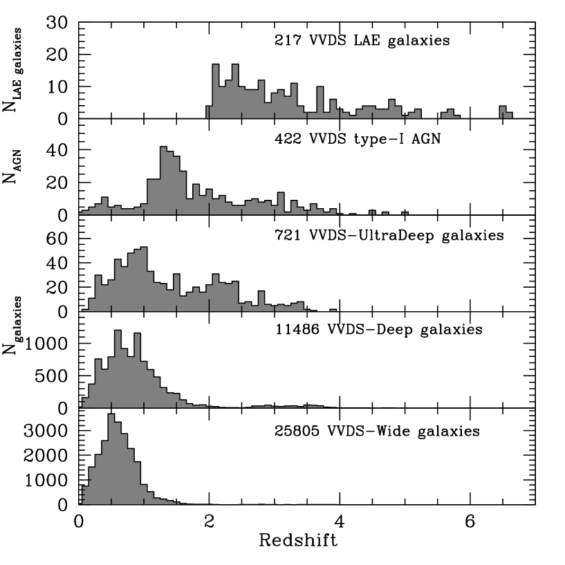
Figure 1: The redshift distributions from the 35 016 galaxies in the VVDS surveys: 25 805 galaxies in the VVDS-Wide (including 3 768 from the VVDS-Deep satisfying the $17.5\leq I_{AB}\leq 22.5$ selection), 11 486 galaxies in the VVDS-Deep, 721 galaxies in the VVDS-UltraDeep (excluding those re-observed from the VVDS-Deep), and 217 Lyman-$\alpha$ emmitters (133 found serendipitously, the other galaxies coming from the Deep and Ultra-Deep samples). The redshift distribution of the 422 type-I AGN found in the VVDS surveys is shown on the top panel.

3 Observations and redshift measurement reliability

3.1 Survey fields and area

The survey fields have been chosen to be on the celestial equator to enable visibility of any two field at any time of the year, at locations with low galactic extinction. The fields positions and the survey modes applied on each are listed in Table 3.

The 0226-04 field is the most observed field in the VVDS hosting most of the Deep and all of the Ultra-Deep surveys. It is included in the CFHTLS (Cuillandre et al., 2012) and XMM-LSS (Pierre et al., 2004) imaging areas, and other multi-wavelength data are available as described in Section 4.5. This field was defined and observed before the Subaru SXDF field which has a field centre only 2 degrees away at 0218-05, leaving only one degree between them, such that joining these two fields with bridging photometry and spectroscopy would offer the possibility for a unique large extragalactic field covering more than 3 deg². This 0226-04 field was to become the COSMOS field (Scoville et al. 2007), but this did not happen at the request of the STScI and ESO directors to limit R.A. overload on these facilities, already committed to the GOODS areas including the ECDFS at R.A.=3h32m. The VVDS-10h field was instead selected as the COSMOS field to be observed with HST, despite having at that time limited multi-wavelength data and multi-object spectroscopy available.

The 2217+00 field is in Selected Area SA22, a well studied area revisited by several spectroscopic surveys (e.g. Lilly et al. 1991, Lilly et al. 1995, Steidel et al. 1998), and the VVDS area is now included in the CFHTLS wide imaging survey, with extended redshifts from the VIPERS survey (Guzzo et al. 2013).

The VVDS-Wide field at 1003+01 has evolved into the COSMOS field (Scoville et al. 2007), which was slightly displaced to 1000+02 to avoid some large galactic extinction areas found when more accurate extinction maps were made available after the initial VVDS field selection and imaging survey. The VVDS field is then partially overlapping and extending the area covered with spectroscopy by the zCOSMOS-Wide survey (Lilly et al. 2007).

The 1400+05 field is a high galactic latitude field, and the ECDFS was added as a reference field with VVDS redshifts made rapidly public to a broad community (Le Fèvre et al. 2004a).

The fields location and covered area for each are indicated in Table 3.

Table 3: VVDS fields and exposure times

$$\begin{array}[]{lllcccccccc}\hline\cr\hline\cr\vskip 3.0pt plus 1.0pt minus 1.0pt\cr Field&\alpha_{2000}&\delta_{2000}&b&l&$Survey mode$&$Area$&$VIMOS setup$&T_{exp}(h)\\ \vskip 3.0pt plus 1.0pt minus 1.0pt\cr\hline\cr\vskip 3.0pt plus 1.0pt minus 1.0pt\cr 1003+01&10h03m00.0s&+01\deg 30\arcmin 00\arcsec&42.6&237.8&Wide&1.9$deg$^{2}&LRRED&0.75\\ 1400+05&14h00m00.0s&+05\deg 00\arcmin 00\arcsec&62.5&342.4&Wide&2.2$deg$^{2}&LRRED&0.75\\ 2217+00&22h17m50.4s&+00\deg 24\arcmin 00\arcsec&-44.0&63.3&Wide&4.0$deg$^{2}&LRRED&0.75\\ \vskip 3.0pt plus 1.0pt minus 1.0pt\cr\hline\cr\vskip 3.0pt plus 1.0pt minus 1.0pt\cr 0226-04$\leavevmode\nobreak\ Deep$&02h26m00.0s&-04\deg 30\arcmin 00\arcsec&-58.0&-172.0&Deep&0.61$deg$^{2}&LRRED&4.5\\ $ECDFS$&03h32m28.0s&-27\deg 48\arcmin 30\arcsec&-54.5&223.5&Deep&0.13$deg$^{2}&LRRED&4.5\\ \vskip 3.0pt plus 1.0pt minus 1.0pt\cr\hline\cr\vskip 3.0pt plus 1.0pt minus 1.0pt\cr 0226-04$\leavevmode\nobreak\ Ultra-Deep$&02h26m28.8s&-04\deg 23\arcmin 06\arcsec&58.0&-172.0&Ultra-Deep&512$arcmin$^{2}&LRBLUE&18\\ &&&&&&&LRRED&18\\ \vskip 3.0pt plus 1.0pt minus 1.0pt\cr\hline\cr\end{array}$$

3.2 VIMOS on the VLT

The VIsible Multi-Object Spectrograph (VIMOS) is installed on the European Southern Observatory Very Large Telescope unit 3 Melipal. It was commissioned in 2002 (Le Fèvre et al. 2003), and has been in regular operations as a general user instrument since then. VIMOS is a wide field imaging multi-slit spectrograph, hence offering broad band imaging capabilities in u,g,r,i, and z bands, as well as multi-slit spectroscopy with spectral resolution ranging from $R\simeq 230$ to $R\simeq 2500$ (1 arc-second slits), and spectral coverage in $3\,600\leq\lambda\leq 10\,000$Å depending on the dispersing element used (grism / VPH). VIMOS also offers a wide field integral field spectroscopy capability in a field ranging from $27\times 27$arcsec² to $54\times 54$arcsec². The global VIMOS throughput at 6 000Å without the detector and dispersing element is an excellent 78%.

The multi-slit spectroscopy capability has been specifically designed to offer a large multiplex, with the number of individual slits/objects observed simultaneously ranging from $\sim 200$ to $\sim 800$ at high to low spectral resolution, respectively. Multi-slit masks are cut in Invar sheets to excellent accuracy (a few microns, less than one hundredth of an arc-second) using a dedicated laser machine (Conti et al. 2001). Besides the global spectrograph throughput, the ability to observe faint targets relies heavily on the sky signal subtraction accuracy. From our multi-slit observations we consistently reach a sky background subtraction accuracy of better than $\sigma_{skyresidual}\simeq 0.1$% of the sky background intensity, even when stacking up to 18h of observations, as shown in Figure 2.

The VVDS Wide and Deep surveys have been conducted with the LRRED grism covering $5500\leq\lambda\leq 9350$Å, while the VVDS Ultra-Deep survey has used the LRBLUE and LRRED grisms to cover $3650\leq\lambda\leq 9350$Å, both with slits one arc-second wide. This provides a spectral resolution $R=230$. At this resolution, the detectors can accommodate 3–4 full length spectra along the dispersion direction, and, given the projected space density of VVDS targets, more than 400 object-slits per pointing have been observed for the Wide survey, and more than 500 object-slits for the DEEP and Ultra-Deep surveys. More details can be found in Le Fèvre et al. (2005a), and Garilli et al. (2008).

Figure 2: Sky background subtraction accuracy expressed as the ratio of the sky subtracted spectrum over the observed sky spectrum, obtained from the 18h stack of VIMOS-LRRED observations for the VVDS-UltraDeep survey.

3.3 Photometric i–band selection: imaging

All the VVDS spectroscopic sample is I–band (Wide and Deep) or i–band (Ultra-Deep) selected. In support of the VVDS an imaging campaign has been conducted at the CFHT using the CFH12K camera, in BVRI bands (Le Fèvre et al. 2004b). The main requirements for this imaging survey was to be deep enough to select targets down to $I_{AB}=22.5$ and to cover a total of 16 deg² for the Wide survey, and reaching down to $I_{AB}=24$ and cover 1 deg² for the Deep survey. Integration times in the I–band of one hour on the Wide survey and 3h on the Deep survey led to limiting magnitudes of $I_{AB}=24.8$ and $I_{AB}=25.3$ at $5\sigma$ in a 3 arc-second aperture (Le Fèvre et al. 2004b). As described in McCracken et al. (2003), the depth of the imaging survey ensures a 100% completeness in detecting objects down to the limiting magnitude of the spectroscopic survey.

For the Ultra-Deep survey, the release no.3 of the CFHT Legacy Survey i–band imaging on the 0226-04 field has been used to select targets down to $i_{AB}=24.75$. The Megacam i–band filter has a bandpass close to but slightly different from the CFH12K I–band used for the Deep and Wide surveys, warranting a specific notation throughout this paper. The imaging depth of the CFHTLS reaches $i_{AB}=25.5$ at $5\sigma$ in a 3 arc-second aperture, sufficiently deep to avoid any imposed imaging selection bias.

The I–band or i–band selections are based on SExtractor (Bertin and Arnouts, 1996) $mag-auto$ a Kron-magnitude approximating a total magnitude. Two-band colors are computed in 3 arcsecond apertures to ensure that the spectral energy distribution of each galaxy is measured in the same physical size in each band, as well as to maximize flux and to minimize the contamination correction residuals from nearest neighbors. Besides the i–band used for target selection, multi-band imaging and multi-wavelength data have been assembled in the VVDS survey fields as described in Section 4.5.

3.4 Spectroscopic data processing, redshift measurement, and reliability flag

The multi-slit spectroscopy data processing has been performed using the VIPGI data processing environment (Scodeggio et al., 2005). It consists of 2D spectra extraction, sky-subtraction, combination of individual 2D spectra, 1D spectra tracing and extraction, wavelength and flux calibration of the 2D and 1D spectra. The redshift measurements have been performed in several steps using the EZ engine developed within the VVDS (Garilli et al., 2010), based on cross-correlation with spectra templates and augmented by knowledge-based software.

The redshifts are measured separately by 2 persons in the team, and reconciled from a face to face confrontation. This confrontation is designed to smooth-out the possible biases of individual observers and produce an homogeneous reliability assessment by means of a flag. Each redshift measurement has a spectroscopic flag associated to it, indicating the probability for this particular redshift to be right. This method was originally pioneered by the CFRS (Le Fèvre et al. 1995), and since then has been used by other major surveys besides the VVDS like zCOSMOS (Lilly et al. 2007) or VIPERS (Guzzo et al. 2013). This probabilistic approach has been proven over these large surveys to be both reliable and easy to handle in terms of evaluating the selection function of the survey with various sampling rates as described in Section 5.2.

The flag may take the following values:

• 4: 100% probability to be correct

• 3: 95–100% probability to be correct

• 2: 75–85% probability to be correct

• 1: 50–75% probability to be correct

• 0: No redshift could be assigned

• 9: spectrum with a single emission line. The redshift given is the most probable given the observed continuum, it has a $\sim 80$% probability to be correct.

These flag probabilities are examined in more details below.

From this basic flag list, more specific flags have been build using a second digit in front of the reliability digit. The first digit can be ”1” indicating that at least one emission line is broad, i.e. resolved at the observed spectral resolution, or ”2” if the object is not the primary target in the slit but happens to fall in the slit of a primary target by chance projection, and hence provides a spectrum. For the VVDS-UltraDeep, we have added a flag 1.5 corresponding to objects for which the spectroscopic flag is ”1”, and the spectroscopic and photometric redshifts match to within $dz=0.05\times(1+z)$.

This statistical method has been extensively tested from independent repeated observations of several hundred objects, consistently providing similar statistical reliability estimates for the different flag categories (Le Fèvre et al. 1995, Le Fèvre et al. 2005a, Lilly et al. 2009, Guzzo et al. 2013).

We have consolidated this redshift probability scheme from several lines of evidence. The duplicate observations obtained in the VVDS-Deep have been presented in Le Fèvre et al. (2005a). About 386 objects have been observed twice in the ECDFS and 0226-04 fields, processed and redshifts measured independently. More recently, 558 objects from the VVDS-Wide have been re-observed with VIMOS in the context of the VIPERS survey (Guzzo et al. 2013), and 88 VVDS galaxies have been observed in the near-IR with VLT-SINFONI for the purpose of the MASSIV survey (Contini et al. 2012), providing fully independent redshift measurements.

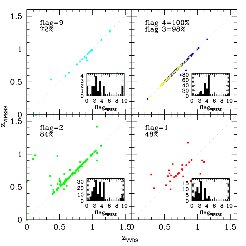
Figure 3: Comparison of independent redshift measurements and classification of 558 galaxies in VVDS-Wide and in the VIPERS survey (Guzzo et al., 2013). The comparison is made for each of the 4 categories of spectra in the VVDS: flags 1, 2, 3 and 4, and 9. The probability for the redshift of each class of galaxy is computed as the fraction of galaxies which agree between VVDS and VIPERS to $|dz|\leq 0.0025\times(1+z)$, and is indicated in the upper left corner of each panel, using as a reference the most reliable redshift flags from the VIPERS survey (the small histogram inset in each panel shows the VIPERS flag distribution). Using only the most reliable flags, the sigma of the redshift difference between VVDS and VIPERS redshift measurements normalized to the expansion factor (1+z) is $\sigma_{dz}=0.00072$ which translates to an individual redshift measurement uncertainty of $\sigma_{v}=202$km/s.

The VIPERS survey uses VIMOS with the red, higher QE, CCDs installed in 2010 with a similar exposure time to the VVDS, hence providing improved S/N at fixed exposure time. We have compared the 558 VVDS redshift measurements in common to VIPERS in Figure 3. For each flag category of galaxies in the VVDS, we compare the VVDS redshift measurements to those of VIPERS, considering that they agree if the velocity difference is $|z_{VVDS}-z_{VIPERS}|\leq 0.0025\times(1+z)$, consistent at $\sim 3\sigma$ with the accuracy in redshift measurement (see below). As VIPERS observations have better S/N than the VVDS we have used the VIPERS galaxies with flags 2, 3, 4 as the exact redshift reference as they have a probability to be right from 94.8 to 100% (Guzzo et al. 2013), and we have defined the probability for a VVDS redshift to be correct as the ratio of galaxies with a redshift agreement between VVDS and these VIPERS galaxies over the total number of galaxies with redshifts for each VVDS flag category. We find the following probabilities that the VVDS redshift measurements are correct: flag 1: 48%, flag 2: 84%, flag 3: 98%, flag 4: 100%, and flag 9: 72%.

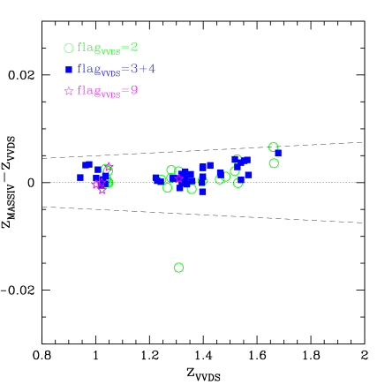
Figure 4: Redshift difference $dz=z_{MASSIV}-z_{VVDS}$ between the independent redshift measurements of the VVDS and MASSIV surveys for 88 galaxies in the VVDS and in the MASSIV survey (Contini et al., 2012). Flags 2 are represented with circles, flags 3 and 4 with squares, and flag 9 with stars. Dashed lines identify $dz=0.0025\times(1+z)$. The sigma of the redshift difference between VVDS and MASSIV redshift measurements normalized to the expansion factor (1+z) is $\sigma_{dz}=0.00072$ which translates to an individual redshift measurement uncertainty of $\sigma_{v}=153$km/s.

The MASSIV survey is a targeted survey to study the kinematic properties of galaxies with $1<z<1.8$ using integral field spectroscopy on the H$\alpha$ line in the J and H bands (Contini et al. 2012). On the 88 galaxies selected from the VVDS, 30, 40, 13, and 5 have flags 2, 3, 4, and 9, respectively. A total of 72 objects have H$\alpha$ or [OIII]5007Å detected at a flux above $2\times 10^{-17}$ erg/s/cm², 16 are not, or only marginally, detected. All of the detected objects but one have the same redshift as measured from the H$\alpha$ or [OIII]5007Å in MASSIV and in the VVDS (Figure 4). For the 16 non detected objects, 2 have a flag 4 among a total of 12 flag 4 observed, 6 have a flag 3 over 40, and 8 have a flag 2 over 30 observed. With the flag 3 and 4 being 98% and 100% correct, we infer that 6 over 52 objects with such flags have not been detected in the SINFONI spectra mainly because the H$\alpha$ or [OIII]5007Å fluxes are below the 4$\sigma$ limit $F(line)\leq 1\times 10^{-17}$ erg/s/cm² (this value is somewhat wavelength dependent because of the varing sky and instrument background). Making the reasonable hypothesis that 15% of the flag 2 objects in MASSIV are undetected for the same reason, we may then deduce that the success rate for redshifts with flag 2 is $(22/30+0.15)$ or 88%. All the 5 galaxies with flag 9 from the VVDS have their redshift confirmed from MASSIV. Combining the 23 VVDS flag 9 galaxies re-observed with MASSIV and VIPERS, we find that 19 have the correct redshift, hence of probability of 83%. We add that another 3 VVDS galaxies at $z\sim 3.5$ have been observed with SINFONI in a pilot program for MASSIV (Lemoine-Busserolle et al. 2010), including 2 flag 3 and one flag 4 object, their redshifts were all confirmed from at least [OIII]5007Å detection.

From the VVDS objects re-observed by VIPERS we derive the velocity difference distribution. The 1-sigma of the distribution normalized to the expansion factor $(1+z)$ is $\sigma_{1+2}=0.00095$, or $\sigma_{1+2}\sim 285$ km/s between two objects, corresponding to a velocity error per object of $\sigma_{v}=\sigma_{1+2}/\sqrt{2}=202$km/s, while for VVDS objects re-observed by MASSIV, we find $\sigma_{1+2}=0.00072$ hence $\sigma_{v}\sim 153$km/s. We find that between VVDS and MASSIV, using fully independent instrument setups, the absolute velocity zero point differs by only $\Delta z=0.0003$. This corresponds to $\sim 40$ km/s at the mean redshift of MASSIV, well within the expected difference given that the measurements are coming from two different instrument systems with different spectral resolutions.

Furthermore, we have re-observed in the Ultra-Deep $\sim 250$ galaxies with flags 0,1,2 from the Deep survey. After 18h integration, most of these flags have become flags 3 or 4. The comparison of redshifts and flags from both the Deep observations and the much deeper Ultra-Deep observations on these galaxies is in full support of the probabilities listed above for each flag, as described in Section 4.3.2.

These measurements of the redshift flag probability are fully in line with our earlier estimates (Le Fèvre et al. 2005a), as well as that observed in other surveys with similar redshift measuring scheme (Le Fèvre et al. 1995, Lilly et al. 2007, Guzzo et al. 2013). This scheme enables a full use of all the galaxies with a redshift and flag measurement, provided appropriate care is given to weight galaxies with different flags when computing volume quantities in relation to the observed parent population, as we discuss in details in Section 5.

Summarizing this section, the VVDS is using a well characterized statistical redshift reliability estimator, which enables a robust statistical treatment of the complete galaxy population with measured redshifts. We demonstrate that the flag 2, 3, 4 and 9 are highly reliable at a level from $\sim 83$% to $100$%. We consider that these objects are forming the best VVDS sample, and we have used it in all the VVDS science analysis. In addition, as the selection function is well defined, objects with flag 1 can also be used despite their 50/50 failure rate. We are therefore quoting the total number of measured redshifts in the VVDS as all objects with a redshift measurement, i.e. with a flag root 1, 2, 3, 4 and 9. The statistical properties of this flag system serve as a basis to the weights defined in Section 5.2, used to derive volume quantities and their associated errors. We invite people using our data release or quoting numbers of observed galaxies with redshifts to take into consideration this powerful statistical redshift measurement treatment.

3.5 Redshift reliability vs. quality

This flag system is sometimes misinterpreted in the literature as an indication of spectra quality (e.g. the recent surveys comparison by Newman et al. 2012, albeit with incorrect numbers regarding the VVDS), but this association is not appropriate. Defining the quality of a single redshift measurement is not as straightforward as it may seem. Several estimators each give a different flavour of ’quality’, like the S/N on the continuum, the number and S/N of emission lines, the strength of the cross-correlation signal. All of these could only be exactly quantified in the presence of constant noise properties as a function of wavelength, but with the highly non-linear background subtraction process, all of these indicators are biased in one way or another. While spectra with high continuum S/N, many spectral lines, a strong correlation signal, lead to a redshift measurement obvious to all observers, faint galaxy surveys going to the limit have to deal with a mixture of these indicators, not always with the best ’quality’ for all indicators. One could get galaxies with a low S/N on the continuum but an obvious set of emission lines matching a single redshift; an emission line may fall on a sky line and be missing while the correlation signal on the continuum is strong; or, importantly, the S/N on the continuum could be low but one could have a strong correlation signal because a number of features are only each weakly detected but add to support the correlation. As a result, ’quality’ assessment is then often subjective, strongly correlated to the individual who made the measurement, and difficult to compare from one survey to another. To the contrary, the probabilistic approach used in the VVDS guarantees an homogeneous treatment of the redshift measurements.

Several different notation schemes or quality estimates have been used in the literature. We contend that they are not of the same nature, and that care must be taken when comparing them. From our VIMOS experience dealing with $>1.5\times 10^{5}$ spectroscopic redshift measurements from the VVDS, zCOSMOS, and VIPERS surveys, it appears that it is illusory to aim at a classification of galaxy redshifts measurements into a scheme as basic as good and bad, but rather that using a more continuous distribution of redshift reliability as described above is more appropriate to this type of dataset.

4 VVDS surveys

4.1 VVDS-Wide

The VVDS-wide has been observing targets selected from their apparent I-band magnitude $17.5\leq I_{AB}\leq 22.5$. A total of 24, 28 and 51 VIMOS pointings have been observed in three fields 1003+01, 1400+05 and 2217+00, respectively. Integration times of 45 minutes have been obtained with the LRRED grism. These observations have been extensively described in Garilli et al. (2008). The final data release presented here adds the observations of 24 more pointings ($\sim 8000$ galaxies) to the Garilli et al. (2008) data. The full VVDS-Wide sample consists of all objects in the three fields 1003+01, 1400+05 and 2217+00, as well as the objects with $17.5\leq I_{AB}\leq 22.5$ in the 0226-04 and ECDFS fields, for a total of $25\,805$ galaxies and $305$ type-I AGN. The total area covered is 8.7 square degrees, the redshift range $0.05\leq z_{Wide}\leq 2$ for a mean redshift $\bar{z}=0.55$ (Le Fèvre et al., 2013) and a volume $\sim 2\times 10^{7}$h^-3Mpc³. As, deliberately, no attempt was made to apply star-galaxy separation algorithms prior to select spectroscopic targets, the VVDS-Wide contains a rather large fraction of 34% of Galactic stars, mainly in the lower Galactic latitude 2217+00 field.

4.2 VVDS-Deep

The VVDS-Deep sample is based solely on I–band selection $17.5\leq I_{AB}\leq 24$. Total integration times of 4.5h have been obtained with the LRRED grism. The VVDS-Deep observations of the 0226-04 field have been extensively described in Le Fèvre et al. (2005a) and the ECDFS in Le Fèvre et al. (2004a).

The VVDS-Deep dataset now includes a sample of $\sim 4000$ additional objects from ’epoch 2’ observations of 8 VIMOS pointings. This sample has been observed and the data processed following the exact same procedure as described in Le Fèvre et al. (2005a). The full field observed from the VVDS-Deep ’Epoch 1’ (Le Fèvre et al. 2005a) and ’Epoch 2’ observations covers 2200 arcmin² as shown in Figure 5.

This brings the total sample of objects observed in the VVDS-Deep to 12 514: 11 486 are galaxies with a spectroscopic redshift measurement and a reliability flag $1\leq flag\leq 9$, 915 are stars and 113 are type I AGN, making this galaxy and AGN sample the largest homogeneous sample with spectroscopic redshifts at this depth. A redshift measurement has not been possible for 1315 objects, bringing the redshift measurement completeness of the full (Epoch 1 + Epoch 2) VVDS-Deep sample to 89.5%. The total area covered is 0.74 square degrees, the redshift range $0.0024\leq z_{Deep}\leq 5$ for a mean redshift $\bar{z}=0.92$ (Le Fèvre et al., 2013), and the volume sampled is $\sim 0.4\times 10^{7}$h^-3Mpc³.

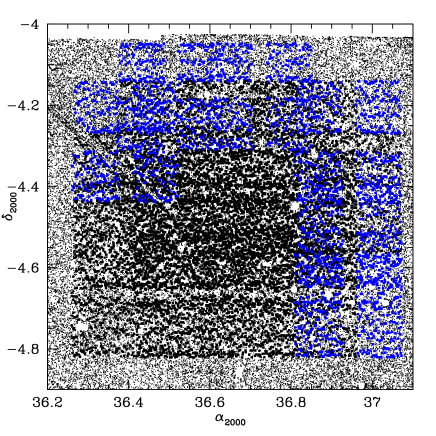
Figure 5: The distribution in ($\alpha,\delta$) of all galaxies observed in the Deep $17.5\leq i_{AB}\leq 24$ sample. Epoch 1 observations are indicated in black heavy symbols, observations from 8 additional VIMOS pointings are indicated in blue, and the photometric parent sample as dots.

4.3 VVDS Ultra-Deep

This latest component of the VVDS was aimed to produce an i-band limited magnitude survey 2.25 magnitudes beyond the VVDS-Wide, and 0.75 magnitudes fainter than the VVDS-Deep, reaching $i_{AB}=24.75$. Very deep spectroscopic observations have been performed in service mode in the framework of ESO Large Program 177.A-0837, integrating 18h per target in each of the LRBLUE and LRRED grisms for 3 VIMOS pointings. These cover a field of 512 arcmin² roughly centered at $\alpha_{2000}=02h26m28.8s$ and $\delta_{2000}=-4^{\circ}23\arcmin 06\arcsec$, included in the VVDS-02h Deep field (0226-04) area, as shown in Figure 6 and listed in Table 4.

To reach the depth of $i_{AB}=24.75$ and ensure a high completeness in redshift measurement, we have devised a strategy with long integrations and an extended wavelength coverage using VIMOS. An essential component to keep a high completeness in measuring redshifts for $z>1$ objects is to reduce redshift degeneracies by increasing the observed wavelength range and therefore maximizing the number of observed spectral features. We elected to combine VIMOS low-resolution blue grism observations over $3650\leq\lambda\leq 6800$Å and low-resolution red grism observations over $5500\leq\lambda\leq 9350$Å to cover a wavelength range 3650 to 9350Å, the overlapping region from 5500 to 6800 Å  then getting a total exposure time of 36 hours.

We have been designing slit masks from the extensive and deep multi-wavelength photometry from the CFHTLS, including three target samples: (i) a randomly selected sample of galaxies with $23\leq i_{AB}\leq 24.75$, (ii) a sample of galaxies with $22.5\leq i_{AB}\leq 24$ randomly selected from galaxies with flags 0, 1 or 2, as measured in the VVDS-Deep sample, and (iii) a sample of ’targets of opportunity’ with objects selected from GALEX Lyman-break (GLBGs) candidates at $z\sim 1$ and extremely red objects (EROs) selected from their red colours and aimed at picking-up high redshift $z>1$ passively evolving red early-type galaxies. In the following we call these samples the ’Ultra-Deep’, the ’Deep-re-observed’, and the ’colour-selected’ samples. The VMMPS mask-design software (Bottini et al., 2005) was first used to force slits on the colour-selected sample (a few per VIMOS quadrant), then to force slits on the Deep-re-observed sample (about 20 per quadrant), and finally to place slits randomly on the Ultra-Deep sample (about 80 per quadrant), for an average total number of about 450 slits observed in one observation.

As described in Section 3.4, the data have been processed using the VIPGI software. The redshift measurements have been performed in several steps using the EZ engine. The redshifts of the blue spectra and the red spectra have been measured separately, each by 2 persons in the team, and two reconciled lists of redshifts derived from the blue and red observations have been separately produced. The 1D blue and red digital spectrograms of each galaxy have then been joined, and redshifts from these combined spectra have been derived again separately by two persons, without knowledge of the redshifts derived from blue or red observations. The final redshifts were then assigned by two persons jointly comparing the three different redshift measurements (blue, red, and joined), and deciding on the associated reliability flags. We have added a new flag ’1.5’ to indicate the spectroscopic redshifts with a low reliability flag=1, but which agree with the photometric redshifts to within $\delta z=0.05\times(1+z)$ (see section 5.1).

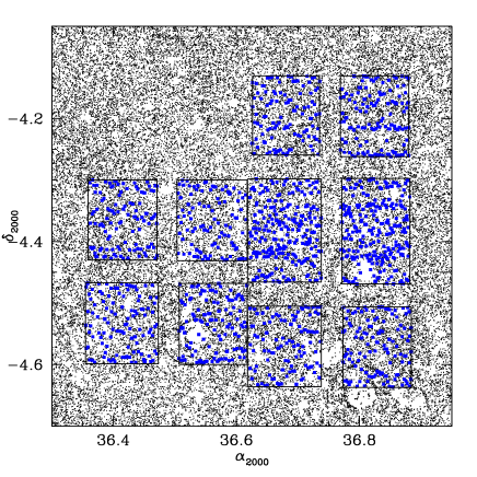
Figure 6: The distribution in ($\alpha,\delta$) of galaxies observed in the Ultra-Deep $23\leq i_{AB}\leq 24.75$ sample (heavy symbols) over the photometric parent sample (dots).

Table 4: VVDS Ultra-Deep observations in the VVDS-02h field

$$\begin{array}[]{p{0.1\linewidth}lllcc}\hline\cr\hline\cr\vskip 3.0pt plus 1.0pt minus 1.0pt\cr Pointing&\alpha_{2000}&\delta_{2000}&$Grism$&$Exposure $&$Seeing $\\ &&&&$time (min)$&\\ \vskip 3.0pt plus 1.0pt minus 1.0pt\cr\hline\cr\vskip 3.0pt plus 1.0pt minus 1.0pt\cr D02P001&02h27m00.72s&-04\deg 16\arcmin 45.3\arcsec&LRRED&40\times 27&1.2\arcsec\\ D02P001&02h27m00.72s&-04\deg 16\arcmin 45.3\arcsec&LRBLUE&40\times 27&1.0\arcsec\\ D02P002&02h27m01.30s&-04\deg 29\arcmin 12.0\arcsec&LRRED&40\times 27&1.2\arcsec\\ D02P002&02h27m01.30s&-04\deg 29\arcmin 12.0\arcsec&LRBLUE&40\times 27&1.1\arcsec\\ D02P003&02h25m57.25s&-04\deg 26\arcmin 54.5\arcsec&LRRED&40\times 27&0.9\arcsec\\ D02P003&02h25m57.25s&-04\deg 26\arcmin 54.5\arcsec&LRBLUE&40\times 27&0.9\arcsec\\ \vskip 3.0pt plus 1.0pt minus 1.0pt\cr\hline\cr\end{array}$$

4.3.1 The Ultra-Deep $23\leq i_{AB}\leq 24.75$ sample

The main Ultra-Deep sample contains a total of 815 objects which have been observed: we have measured the redshifts for 721 galaxies, 3 type-I AGN, and 23 stars, 673 of which have a flag larger or equal to 1.5, representing $\sim 83$% of the sample. The total area covered is 0.14 square degrees, the redshift range is $0.05\leq z_{Ultra-Deep}\leq 4.5$ for a mean redshift $\bar{z}=1.38$ (Le Fèvre et al., 2013), and the volume sampled is $0.5\times 10^{6}$h^-3Mpc³.

4.3.2 The re-observed deep $17.5\leq i_{AB}\leq 24$ sample

In these deeper Ultra-Deep observations, we have re-observed the galaxies in the original VVDS-Deep (Le Fèvre et al. 2005a) for which we failed to get redshifts (flag 0), those with lower reliability (flag 1), and have re-observed a sample of galaxies with higher redshifts reliability (flag 2) to further assess their statistical robustness. The main goal was to get secure spectroscopic redshifts for these objects, and hence obtain a statistical estimate of the true redshift distribution of the galaxies in the VVDS-Deep which had lower redshift reliability flags. This sample has been randomly build from the objects with flags 0, or with flags 1 and 2 and redshifts $z\geq 1.4$ in the Epoch-1 VVDS-Deep sample. This redshift $z=1.4$ marks the point when the [OII]3727Å line starts to be difficult to detect as the LRRED sensitivity and strong sky OH bands affect this line above $\sim 9000$Å, and at $z=1.5$ this line is beyond our wavelength domain, leaving only weak absorption features from the UV-rest spectrum in the observed domain.

A total of 241 objects have been successfully targeted. The deeper observations enable to secure a large number of redshifts for these sources, with 153 objects with a very high reliability flag above 3, and 72 objects with a reliable flag from 1.5 to 2.5.

These new measurements enable to better understand the incompleteness of the VVDS-Deep sample, as discussed in section 5.4. The redshift distribution of this sample, for each original VVDS-Deep flag, is presented in Figure 7. The redshift distribution of VVDS-Deep galaxies with flag=0 shows that the redshift failures in VVDS-Deep are coming from the full redshift range, although with a preference for $1<z<2.5$ including the LRRED grism ’redshift desert’ (see Section 5.5). The re-observed flag 1 and flag 2 are also preferentially in this ’redshift desert’, as expected because the wavelength range of the LRRED grism makes it difficult to identify features in this difficult redshift range.

Using this re-observed VVDS-Deep sample has enabled a statistical correction of the full sample using the weighting scheme described in Section 5.

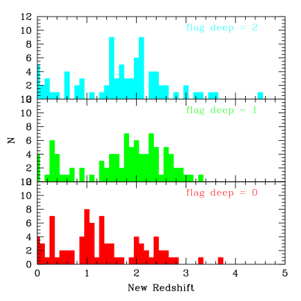
Figure 7: The redshift distribution of objects with spectroscopic flags 0, 1 and 2 from the VVDS-Deep sample with $17.5\leq i_{AB}\leq 24$, re-observed in the VVDS-UltraDeep survey.

4.4 Serendipitous observations of Lyman Alpha Emitting galaxies

As we were processing 2D spectra of the main targets of this program, a number of objects with single emission lines have been identified falling at random positions along the slits. This is not surprising given the depth of the survey, and, as the slits extend into blank sky areas, the high number of slits implied a large serendipitous survey of a significant sky area. For the VVDS-Deep observations of the 0226-04 field, the total sky area observed through the slits is 22 arcmin², while for the Ultra-Deep observations in 3 masks the total sky area amounts to a total of 3.2 arcmin². The majority of these single emission line objects have been identified as Lyman–$\alpha$ emitters with redshifts $2\leq z\leq 6.62$, as described in Cassata et al. (2011).

4.5 Multi-wavelength data in the VVDS surveys

The VVDS surveys have been conducted in fields with a large range of multi-wavelength data, as summarized here.

The VVDS-Wide fields have been observed with the CFH12K camera at CFHT (Le Fèvre et al. 2004a), reaching depth of $I_{AB}=24$ ($3\sigma$) (McCracken et al. 2003). All VVDS-Wide fields have BVRI photometry, except the 1400+05 which has BRI photometry.

The VVDS-02h 0226-04, including the Deep and Ultra-Deep surveys, has been the target of a number of multi-wavelength observations. Improving on the early CHF12K BVRI survey described above and U-band imaging (Radovich et al., 2004), the CFHT Legacy Survey (CFHTLS, Cuillandre et al. 2012) D1 field is including all of the VVDS-02h area observed in the u’gri and z filters with the Megacam at CFHT, with seeing FWHM from 0.75 to 0.99 and reaching 50% completeness magnitude for point sources at depths of 26.96, 26.73, 26.34, 25.98, and 25.44 in these bands, respectively. Following the initial survey of Iovino et al. (2005) and Temporin et al. (2008) in this field, new near-infrared photometry has become available from the WIRDS survey (Bielby et al. 2012), reaching 50% completeness for point-sources at $J_{AB}=24.90$, $H_{AB}=24.85$ and $Ks_{AB}=24.80$ with 0.80, 0.68, 0.73 arcsec seeing FWHM images respectively. Other multi-wavelength data are available in this field, with GALEX (Arnouts et al. 2005), XMM (Pierre et al. 2004), Spitzer-SWIRE (Lonsdale et al. 2003), and VLA (Bondi et al. 2003). This field has been the target of the Herschel HERMES survey (Oliver et al. 2012), and matched to VVDS data (Lemaux et al. in preparation).

The VVDS-22h 2217+00 field has been receiving additional photometric observations since the VVDS imaging completion. Near infrared imaging in J and K bands reaching $K=21$ (Vega) has been obtained by the UKIRT UKIDSS-DXS survey (Lawrence et al. 2007). This field has been extensively imaged in u’,g,r, i, and z bands by the CFHTLS over an extended area named CFHTLS-W4 covering a total of 25 square degrees in a SE-NW oriented stripe.

All the multi-wavelength data has been cross-correlated with the VVDS spectroscopic sample and is made available on the VVDS database.

5 Completeness and selection function

5.1 Photometric redshifts of the full sample

To help understand the spectroscopic completeness, we are using photometric redshifts computed following the method described in Ilbert et al. (2006) and Ilbert et al. (2009). We have used the CFHTLS data release v5.0, with u’,g,r,i and z’ photometry reaching 80% magnitude completeness limits for point sources of 26.4, 26.1, 25.6, 25.3, 25.0, respectively. We have added near-IR photometry from the WIRDS survey in J H and Ks bands (Bielby et al., 2012). The photometric redshifts have been trained on a spectroscopic sample including the highly reliable (flags 3 and 4) spectroscopic redshifts from the VVDS-Deep (Le Fèvre et al. 2005a) and new spectroscopic redshifts with flags 3 and 4 from the Ultra-Deep survey, following the method described in Ilbert et al. (2006). The comparison of spectroscopic redshifts and photometric redshifts is shown in Figure 8.

We find that there is an excellent agreement between the spectroscopic and photometric redshifts with $dz=0.05\times(1+z)$. The rate of photometric redshifts catastrophic failures is below 3% for all flags. There is a small number of catastrophic failures in the redshift range $2\leq z\leq 3.5$, including objects with very secure spectroscopic redshifts (flags 3 and 4), this is due in part to objects for which the NIR photometry is lacking (e.g. on masked areas in the NIR images).

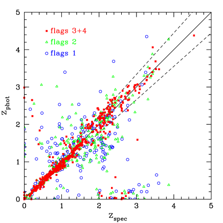
Figure 8: Comparison of photometric and spectroscopic redshifts, for different spectroscopic flags. The dashed lines represent agreement between the two within $|dz|\leq 0.05\times(1+z)$. Filled (empty) symbols are for galaxies with (without) JHK photometry, respectively.

5.2 Sampling rates

The selection function of a spectroscopic redshift survey proceeds from different steps in constructing the final sample, starting from the photometric sample from which targets are selected. To describe the completeness of the VVDS we make use of the following definitions. $N_{phot}^{full}$ is the number of objects in the full photometric catalogue limited by the magnitude range of the survey: $17.5\leq I_{AB}\leq 22.5$ for the Wide survey, $17.5\leq I_{AB}\leq 24$ for the Deep, and $23\leq i_{AB}\leq 24.75$ for the Ultra-Deep. $N_{phot}^{parent}$ is the number of objects in the parent catalogue used for the spectroscopic target selection that corresponds to the full photometric catalogue after removing the objects already observed in this area. $N_{target}$ is the number of targets selected for spectroscopic observations and $N_{spec}$ is the number of objects for which one is able to measure a spectroscopic redshift (using the flag system described in Section 3.4).

With this formalism, we can easily define the completeness of the VVDS spectroscopic samples as the combination of three different sampling rates, as described below.

As the VVDS is purely magnitude selected, the first sampling to consider is the fraction of objects targeted compared to the number of objects in the full photometric catalog, as a function of i-band magnitude. We call this the Target Sampling Rate (TSR) defined as the ratio $N_{target}$/$N_{phot}^{parent}$. This ratio does not depend on the magnitude of the sources, as the VVDS targets have been selected totally randomly within the parent photometric catalogue. The TSR varies with position on the sky, as described in Section 5.6. The weight associated to the TSR is $w_{TSR}=1/TSR$.

A second factor to take into account is the Spectroscopic Success Rate (SSR), the ratio $N_{spec}$/$N_{target}$. It is a function of both the selection magnitude and redshift. To determine the dependence of SSR on redshift, we use the spectroscopic redshift for the targets that yield a redshift, and the photometric redshift for all the other targets. The weight associated to the SSR is $w_{SSR}=1/SSR$.

The third factor is the photometric sampling rate (PSR), computed as the ratio $N_{phot}^{parent}$/$N_{phot}^{full}$. It applies only for the Ultra-Deep survey as some of the brighter objects had already been observed on the Deep survey. The weight associated to the PSR is $w_{PSR}=1/PSR$. For the Wide and Deep surveys $w_{PSR}=1$.

We expand below on the completeness computation for the VVDS-Deep sample, as it can be further refined using the VVDS-Deep galaxies re-observed in the VVDS-UltraDeep. The TSR, defined as $N_{target}$/$N_{phot}^{full}$ ($N_{phot}^{full}=N_{phot}^{parent}$ for VVDS-Deep), is not strictly constant because the VVDS-Deep targeting strategy was optimized to maximize the number of slits on the sky, slightly favouring the selection of small objects, with a size significantly smaller than the slit length. As a consequence, the TSR depends on the x-radius of the objects, the projection of the angular size of the objects on the slit (for further details we refer the reader to Ilbert et al. 2005). The SSR of the re-observed VVDS-Deep needs a more detailed treatment. It is defined as above ($N_{spec}$/$N_{target}$), but the redshift distribution of objects with flag=1,2,9 is corrected using both photometric redshifts and the spectroscopic redshifts of the objects that were re-observed with deeper integration and larger wavelength coverage in the VVDS Ultra-Deep (see Sect. 4.3.2). We used the remeasured redshifts as follows. A sample of $\sim 80$ objects with flag=1 and $\sim 80$ with flag=2 in the original VVDS-Deep were re-observed in the VVDS-UltraDeep, and furthermore these objects were selected with spectroscopic redshift $z_{VVDS-Deep}\geq 1.4$. We computed the $n(z)$ distribution of these objects using the re-observed redshift values, and we rescaled it to the total number of flag 1 and 2 objects (in the VVDS first+second Epoch data) with $z\geq 1.4$. We did it separately for flag 1 and 2, and we call these distributions $n_{1,\geq 1.4}(z)$ and $n_{2,\geq 1.4}(z)$. Then we used the photometric redshifts (see Sect. 5.1) to compute the $n(z)$ of flag 1 and 2 objects with spectroscopic redshift $<1.4$, as these are demonstrated to be secure to $i_{AB}\leq 24$ (e.g. Ilbert et al., 2006). We call these distributions $n_{1,<1.4}(z)$ and $n_{2,<1.4}(z)$. Summing the two new $n(z)$ (for $z<1.4$ and $z\geq 1.4$) for each flag we obtain the total redshift distributions for the two classes of objects, and we consider them 100% correct. We call them $n_{1,corr}(z)$ and $n_{2,corr}(z)$. For each class of flag 1 and 2 we then obtain the original $n_{1}(z)$ and $n_{2}(z)$, made using the original spectroscopic redshifts, and the corrected ones $n_{1,corr}(z)$ and $n_{2,corr}(z)$, made using a combination of remeasured spectroscopic redshifts and photometric redshifts. We computed the corrected redshift distribution also for flag=9 objects ($n_{9,corr}(z)$). We do not have re-observed spectra for this class of targets, so $n_{9,corr}(z)$ is simply their photometric redshift distribution, as this is very robust in this redshift range (see Section 5.1, Ilbert et al. 2009, and the comparison to MASSIV redshifts in Section 3.4). We call M_n(z),i the ratio $n_{i}(z)$/$n_{i,corr}(z)$, where i=1,2,9 (according to the flag). We note that M_n(z) is a modulation of the original $n(z)$, so it does not change the total number of objects. On the contrary, both the TSR and SSR are needed to take into account missed objects. To derive the $N_{spec}$ and $N_{target}$ as a function of redshift we weighted flag=1,2,9 objects by $w_{M,i}=1/M_{n(z),i}$ (where i=1,2,9) while we do not apply any weight to the counts of flag=3 and 4 objects. To compute $N_{target}$ as a function of $z$ we also need the $n(z)$ of flag=0 objects. We use the $n(z)$ of the re-observed flag=0 (see Sect. 4.3.2), normalized to the total number of flag=0 in our sample. We finally computed the $SSR=N_{spec}$/$N_{target}$ as a function of both magnitude and redshift, using the remodulated $N_{spec}$ and $N_{target}$. It is important to note that, when using the $n(z)$ of photometric redshifts, we corrected it for the failure rate in the determination of photometric redshifts themselves. We computed the failure rate as the ratio between the spectroscopic $n(z)$ of objects with flag=3 and 4, and their photometric $n(z)$ (Section 5.1).

5.3 Selection function for the Ultra-deep sample

The PSR, TSR and SSR for the Ultra-Deep sample are shown in Figures 9 and 10. The PSR is rising with magnitude, starting at $PSR\sim 0.7$ as the VVDS-Deep observations reduce the available number of targets, and reaching PSR=1 above $i_{AB}=24$, a magnitude range where no galaxies had been observed in previous observing campaigns. The TSR is constant with magnitude, indicating that 6.5% of objects with $23\leq i_{AB}\leq 24.75$ have been observed in spectroscopy. The SSR is more complex: as magnitude increases the SSR gets globally lower and the success rate varies with redshift. At redshifts up to $z\sim 1.2$ the SSR goes from 1 at the bright end to $\simeq 0.8$ at the faint end, a possible result of the lack of emission features in these objects. In the range $1.2<z<2$, the SSR is starting at $SSR\sim 0.9$ and is getting worse to $SSR\sim 0.6$ at $z\sim 1.5$ in the faintest magnitude bin. With the large wavelength coverage observed, we can see that the ’redshift desert’ is being crossed without much difficulty, but the range $1.5\leq z\leq 2$ is still affected by some incompleteness. The redshift range above $z\sim 2$ benefits from a higher SSR of $0.8<SSR<1$, the result of the combined large wavelength coverage following the key spectral features at these redshifts; above $z=2.5$ the SSR gets down to $\sim 0.8$ only in the faintest magnitude bin.

Globally, the success rate in determining redshifts for this very faint sample is quite high at 80%, which ensures that no major population has escaped detection. We show in Figure 11 the rest U-V colour distribution of the failed sample with flags 0 and 1: the colour distribution of the failed population is not significantly different from the overall population.

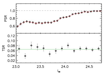
Figure 9: Photometric Sampling Rate (PSR, top) and Target Sampling Rate (TSR, bottom) vs. magnitude for the redshift measurement of the Ultra-Deep $23\leq i_{AB}\leq 24.75$ sample.

Figure 10: Spectroscopic Success Rate (SSR) for the redshift measurement of the Ultra-Deep $23\leq i_{AB}\leq 24.75$ sample, in bins of increasing magnitude, and as a function of redshift.

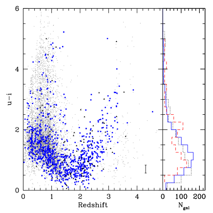
Figure 11: Observed $u-i$ colour distribution vs. redshift of the lowest reliability population (flags 1, black squares) compared to the distribution of galaxies with reliable redshifts (blue squares) for the Ultra-Deep $23\leq i_{AB}\leq 24.75$ sample. The distribution of colours vs. redshift in the Deep sample is shown in grey, and the typical $u-i$ error bar is shown on the lower right corner. The projected colour distribution is shown on the right panel as the blue histogram for reliable redshifts (2,3,4,9), the black dotted histogram for the lowest reliability population (flags 1) multiplied by 10 for comparison, and the red dashed histogram for the population of failed redshifts (flags 0) multiplied by 20 for comparison.

5.4 Selection function for the Deep sample

The TSR and SSR for the Deep sample are shown in Figures 12 and 13. The PSR is irrelevant (PSR=1) for this sample. The TSR is ranging from 0.13 to 0.29 with a mean of 0.261, reflecting the areas where we observed 1, 2 or 4 times with VIMOS, and is varying with the radius of the object along the slit as shown in Figure 12. The SSR is varying as a function of magnitude and redshift (Figure 13). For the faintest magnitudes it is ranging from 0.92 at $z\sim 1$ to 0.7 at $z\sim 2.3$. In addition, we have corrected for the variation of the flag reliability with redshift, computing the weight $w_{129}$ as the ratio of the galaxies with the lower reliability flags 1, 2 and 9 over the number of galaxies with photometric redshifts and re-observed spectroscopic redshifts in the same redshift bin, as shown in figure 14. While this ratio is constant at 1 up to $z\sim 1.6$, independently of magnitude, it is significantly lower than one in the range $1.6<z<2.7$ and becomes higher than one for $z>2.7$, correcting for the fact that spectroscopic redshifts with low reliability flags have been assigned preferentially at $z>2.7$ than in the redshift desert $1.6<z<2.7$.

Figure 12: Target Sampling Rate (TSR) for the redshift measurement of the Deep $17.5\leq I_{AB}\leq 24$ sample, as a function of the projected size of objects along the slit.

Figure 13: Spectroscopic Success Rate (SSR) for the redshift measurement of the Deep $17.5\leq I_{AB}\leq 24$ sample

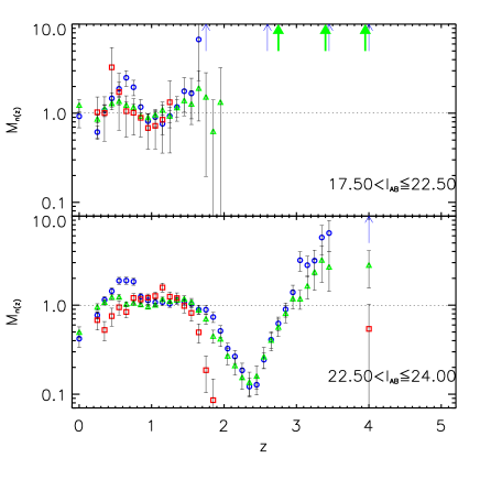
Figure 14: Modulation M_n(z) of the redshift distribution of flag=1 (blue circles), flag=2 (green triangles) and flag=9 (red squares) galaxies. See text for the definition. The two panels represent two magnitude ranges, as indicated in the labels. Arrows indicate when the value of $M_{n(z)}$ is larger than 10: for $z>1.7$ in $17.5\leq I_{AB}\leq 22.5$ and for $z>3.5$ in $22.5\leq I_{AB}\leq 24$ for flag=1 (thin blue arrows), and for $z>2.7$ in $17.5\leq I_{AB}\leq 22.5$ for flag=2 galaxies (thick green arrows). We do not have flag=9 galaxies for $z>1.5$ in $17.5\leq I_{AB}\leq 22.5$ and for $2<z<3.5$ in $22.5\leq I_{AB}\leq 24.$.

5.5 Effect of wavelength domain on redshift completeness

In the complex spectroscopic redshift measurement process, the observed wavelength domain plays a critical role. In order to evaluate the impact of the wavelength coverage on redshift measurements we compare in Figure 15 the redshifts obtained using either the blue (LRBLUE, 3650–6800Å) or red (LRRED, 5500–9350Å) VIMOS setups, and in Figure 16 we show the comparison between redshifts derived from the VIMOS blue or red setups and the final galaxy redshifts obtained when using the full wavelength domain 3650–9350Å. It is clearly seen that with the red setup alone, there is a trend for galaxies with low reliability flags with $z>1.5$ to have their redshifts overestimated. This is directly related to [OII]3727 leaving the observed wavelength domain, leaving only weak features as redshift increases until the Ly$\alpha$ line would enter this wavelength domain at $z>3.5$. On the other hand, using the blue setup alone, galaxies with low reliability flags and redshifts in the range $1.5\leq z\leq 2.5$, have underestimated redshifts. We can also see very well that combining the blue and red wavelength observations to expand the wavelength coverage is needed to cross the ’red redshift desert’ at $2.2\leq z\leq 2.8$ produced by the red wavelength coverage missing out on the 1215–1900Å rest frame domain rich in spectral features (Ly$\alpha$, CIV-1549, etc.), and the ’blue redshift desert’ at $0.8\leq z\leq 1.5$ produced by the blue wavelength coverage corresponding to the absence of the 3727–4000Å domain (with [OII]3727, CaH+K, 4000Å break, etc.). This is best seen in comparing the redshift distributions of the most reliable redshift measurements (flags 3 and 4) for each setup, as shown in Figure 17, where the complementarity of these two wavelength domains is fully evident.

This experience of performing the observations of the same galaxies with a blue and a red setup with the VIMOS spectrograph and independently measuring redshifts with blue, red or a full wavelength coverage 3650–9350Å therefore clearly demonstrates the benefit of using a large range covering most of the visible domain. It is clear from our analysis that surveys using only a partial wavelength coverage in the 0.35–1 micron domain, like the DEEP2 in $6500-9100$Å, the VVDS-Deep and VVDS-Wide using $5500-9300$Å (this paper) or the zCOSMOS-faint using $3600-6800$Å (Lilly et al. 2007), might be subject to observational biases that must be carefully evaluated in terms of their spectroscopic success rate varying with magnitude but also with redshift, as we have discussed in previous sections for the VVDS surveys.

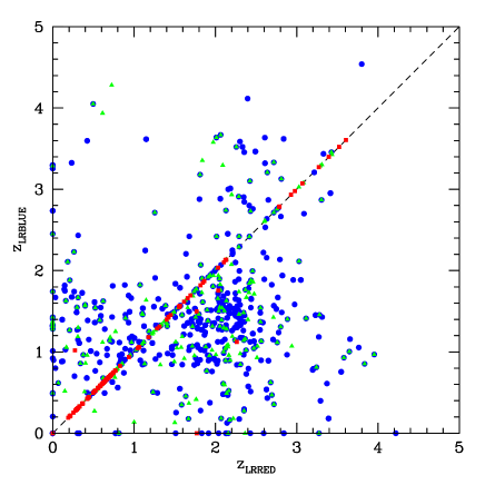
Figure 15: Comparison of redshifts measured from the LRBLUE 3650–6800Å VIMOS grism with redshifts obtained using the LRRED 5500–9350Å grism (red squares: flags 3, 4 and 9; green triangles: flag 2; blue circles: flags 1)

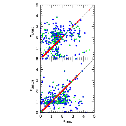
Figure 16: Comparison of redshifts measured from the LRBLUE 3650–6800Å VIMOS grism (bottom) or from the LRRED 5500–9350Å grism (top) with the best redshifts using the full LRBLUE+LRRED 3650-9350Å wavelength domain (red squares: flags 3, 4 and 9; green triangles: flag 2; blue circles: flags 1).

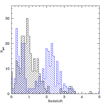
Figure 17: Redshift distribution of galaxies with the most reliable redshifts (flags 3 and 4), from the LRBLUE setup (hatched blue histogram), and from the LRRED setup (hatched black histogram).

5.6 Spectroscopic and photometric masks

The selection of targets in the ($\alpha,\delta$) plane proceeds from the combination of the geometric constraints from the photometric catalogs and the placement of slits in the slit mask-making process. The knowledge of the spatial selection of targets is an important part of the selection function, e.g. for clustering analysis (de la Torre et al. 2011) or group finding (Cucciati et al. 2010).

The photometric catalogs are carefully screened to identify regions where the photometry is potentially affected, e.g. by bright stars and their halos, satellite trails, detector defects, and this information is stored in photometric region files. The spectroscopic slit-masks design leads to geometric constraints (see Le Fèvre et al. 2005a) which, depending on the number of observations at a given sky location, will create a TSR varying with ($\alpha,\delta$). This is stored in spectroscopic region files indicating the $TSR(\alpha,\delta$).

The photometric and spectroscopic region files are made available as part of the final VVDS release.

5.7 Correcting for the selection function

The VVDS sample can be corrected for the selection function described in previous sections, counting each galaxy with the following weight $W_{gal,i}$:

$W_{gal,i}=1/_{PSR}\times 1/_{TSR}\times 1/_{SSR}\times 1/w_{129}$

with $PSR$, $TSR$, $SSR$, and $w_{129}$ as described in Section 5.2. This provides corrected counts, and therefore forms the baseline for volume–complete analysis in the VVDS. The luminosity function and star-formation rate evolution presented in Cucciati et al. (2012), has used the latest VVDS weights as presented here. The redshift distribution of magnitude limited samples at various depth, corrected from selection effects, is presented and discussed in Le Fèvre et al. (2013).

6 Properties of galaxies in the VVDS

6.1 The final VVDS sample

The observations presented in this paper complete the VIMOS VLT Deep Survey. In all, the redshifts of a purely I-band magnitude limited sample of 35 016 extragalactic sources have been obtained, including the redshifts of 34 594 galaxies and 422 type I AGNs, as described in Table 1. The number of galaxies in several redshift ranges are provided in Table 2. We note the large redshift coverage of the VVDS, with redshifts of galaxies ranging from $z=0.0024$ to $z=6.62$, and type-I AGN from $z=0.0224$ to $z=5.0163$. In particular, the VVDS has assembled an unprecedented number of 933 galaxies with spectroscopic redshifts through the ’redshift desert’ $1.5<z<2.5$.

In addition to the extragalactic population, a total of 12 430 galactic stars have an observed spectrum. This results from the deliberate absence of photometric star-galaxy separation ahead of the spectroscopic observations to avoid removing compact extragalactic objects. While galactic stars represent a high 34% fraction of the wide survey, they represent only 8.2% and 3.2% of deep and Ultra-Deep samples, respectively, a modest cost to pay to be able to retain all AGNs and compact galaxies in our sample.

6.2 NIR–selected samples with spectroscopic measurements complete to $J_{AB}=23$, $H_{AB}=22.5$ and $Ks_{AB}=22$

With the depth of the Ultra-deep sample to $i_{AB}=24.75$ and the distribution of $I-J$, $I-H$ and $I-K$ colours, we are able to build samples nearly complete in spectroscopic redshift measurements with 5 846, 5 207, and 4 690 galaxies with $J_{AB}\leq 23$, $H_{AB}\leq 22.5$, and $Ks_{AB}\leq 22$, respectively, as shown in Figure 18. At these limits only a few percent of the reddest galaxies (e.g. with $i-Ks_{AB}>3$) would escape detection. Fainter than this limit, the completeness is still 80% at $Ks_{AB}=23$ loosing only the redder objects with $i-Ks_{AB}\geq 2$, and extends down to $Ks_{AB}=24$ for star forming objects with $i-Ks_{AB}\leq 1$.

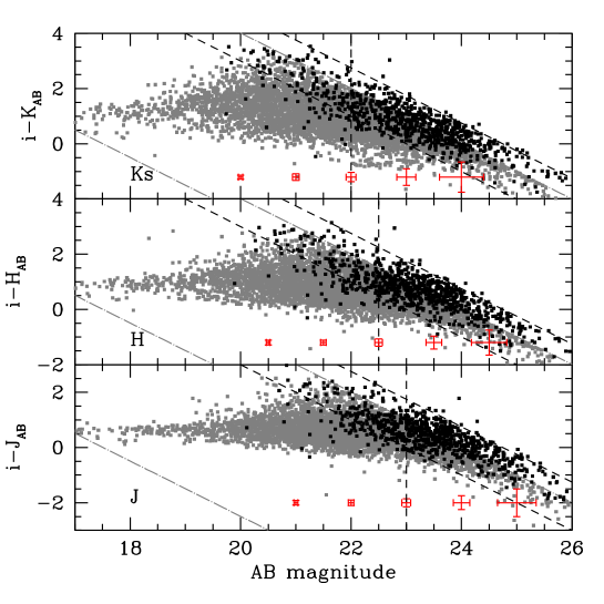
Figure 18: NIR colour magnitude diagram for J, H and Ks selected samples obtained from the Ultra-Deep sample (black points): The two oblique dashed lines correspond to the I-band limiting magnitudes of the survey $i_{AB}=23$ on the bright end, $i_{AB}=24.75$ on the faint end. The VVDS-Deep colour-magnitude distribution is shown as the grey points with the $i_{AB}=17.5$ and $i_{AB}=24$ limits indicated as long-dashed lines. We are able to extract samples nearly complete in spectroscopic redshift measurements, selected down to $J_{AB}=23$, $H_{AB}=22.5$, and $Ks_{AB}=22$ (vertical dashed lines). The faint i-band magnitude cut imposes a loss of red objects for fainter magnitudes but still 80% complete down to $J_{AB}=24$, $H_{AB}=23.5$, and $Ks_{AB}=23$. Typical error bars are shown at the bottom of each panel.

6.3 Magnitude-redshift distributions

The apparent $I_{AB}$ magnitude as a function of redshift for the VVDS Wide, Deep and Ultra-Deep samples shows the imposed magnitude limits as presented in Figure 19. The complementarity of the three samples is evident, with the bright part of the luminosity function best sampled in the Wide and Deep samples, the deep and Ultra-Deep samples sampling the faint population, and the Ultra-Deep sample being mostly unaffected by any instrument-imposed redshift desert.

The distribution of absolute rest-frame u-band and B-band magnitudes in the Deep and Ultra-Deep samples are presented in Figure 20. At redshift $z\sim 1$ the VVDS surveys span a luminosity range from $M_{B}\sim-18$ to $M_{B}\sim-23$, corresponding to 0.07 up to more than $7\times$ the characteristic luminosity $M^{*}$ (Ilbert et al. 2005, Cucciati et al. 2012).

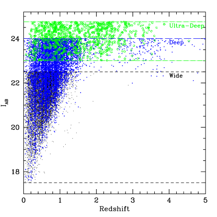
Figure 19: Distribution of apparent $I_{AB}$ apparent magnitudes for the the VVDS-Wide (dots), VVDS-Deep (squares) and Ultra-Deep (open circles) samples.

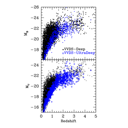
Figure 20: Distribution of B-band (top) and u-band (bottom) absolute magnitudes for the VVDS-Deep (dots) and Ultra-Deep (open circles) samples.

6.4 Colour - magnitude evolution

The $M_{u}-M_{r}$ vs. $M_{r}$ colour magnitude diagrams for the VVDS-Deep and Ultra-Deep samples are presented as a function of redshift in Figure 21. As already noted from our earlier sample by Franzetti et al. (2007), the VVDS data show a clear bimodality in colour, already present from redshifts $1.5<z<2$, with a second peak in $M_{u}-M_{r}$ starting to be prominent at $1<z\leq 1.5$ and below. The VVDS traces up to $z\sim 2$ the ’red sequence’ originally identified in Bell et al. (2004) up to $z\sim 1$.

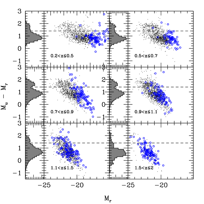
Figure 21: $M_{u}-M_{r}$ vs. $M_{r}$ colour-magnitude diagram for the VVDS-Deep (dots) and VVDS-UltraDeep (circles). A colour bimodality is observed up to $1<z<1.5$.

6.5 Average spectral properties

The average spectra of galaxies in the VVDS are presented in Figures 22 and 23. We have used the odcombine task in IRAF, averaging spectra after moderate sigma clipping and scaling to the same median continuum value, and applying equal weight to all spectra.

These spectra average over the range of spectral types, which cover from early-type to star-forming galaxies.

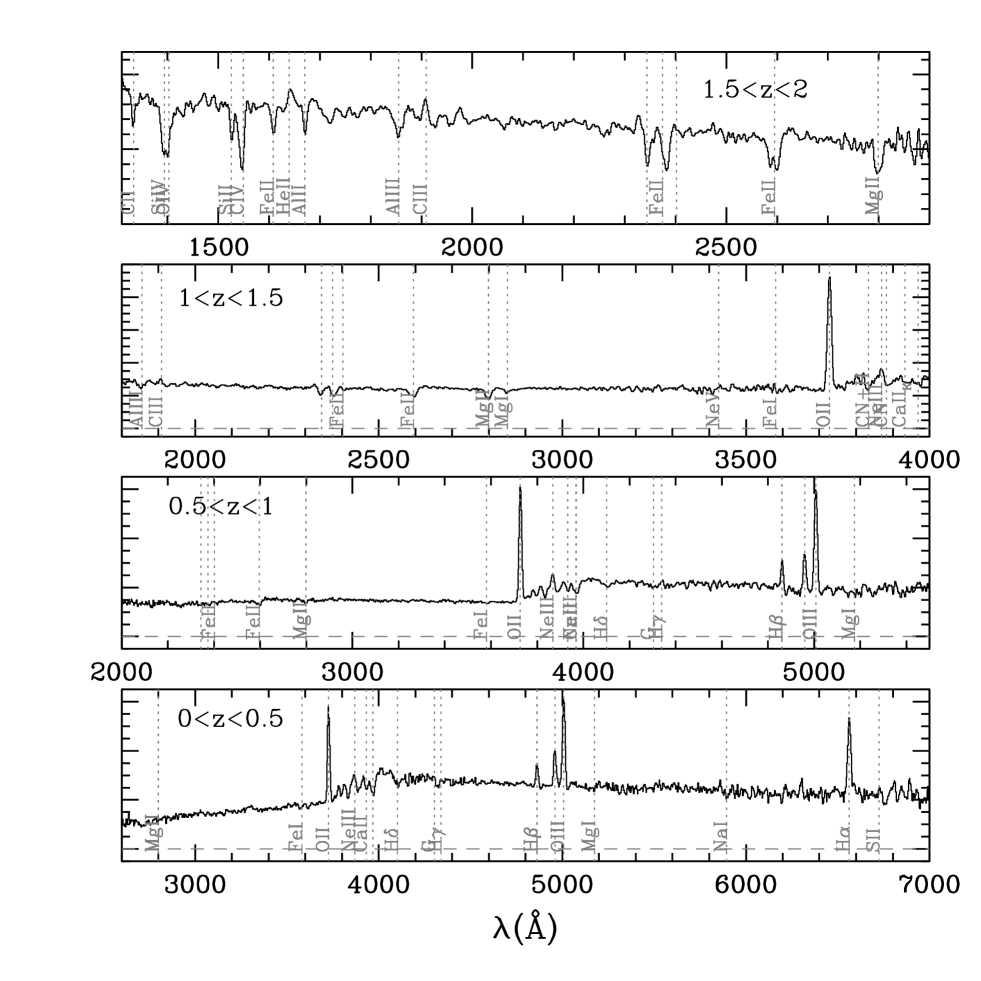
Figure 22: Average rest-frame spectra ($F_{\lambda}$) of all galaxies with flags 3 and 4 in the VVDS per redshift bin up to $z=2$.

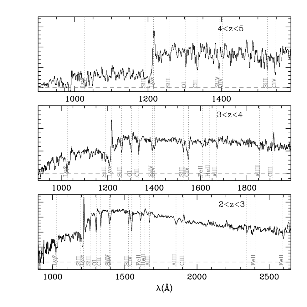
Figure 23: Average rest-frame spectra ($F_{\lambda}$) of all galaxies with flags 2, 3 and 4 in the VVDS per redshift bin from $z=2$ to $z=5$.

7 Comparison with other spectroscopic surveys at high redshifts

Comparing different spectroscopic redshift surveys is not as straightforward as it may seem, as the parameter space defining them is quite large, and the science goals may significantly differ. Different flavours of multi-object spectrographs (MOS) enable different types of surveys, covering different parts of the observing and science parameter space, hence special care must be taken when comparing surveys. The most important survey output parameters are the number of galaxies observed, the limiting magnitude, the sky area or volume covered and the redshift range surveyed. These are directly related to the technical performances of each MOS, including the instrument field of view, the wavelength coverage, the throughput, the number of simultaneous objects that can be observed (multiplex) and the spectral resolution. In addition, the sample selection function is obviously of fundamental importance. If the goals of the survey are more oriented towards galaxy evolution, then a proper sampling of the luminosity and/or mass functions is of primary importance, while for surveys more oriented towards large scale structures and cosmological parameters a fair sampling of all scales in large volumes is a prime concern. In this context, attempts to rationalize a survey performance using information theory, counting the number of bits of information, are largely illusory and it is much more useful to seek complementarity between surveys in a multi–dimensional performance space.

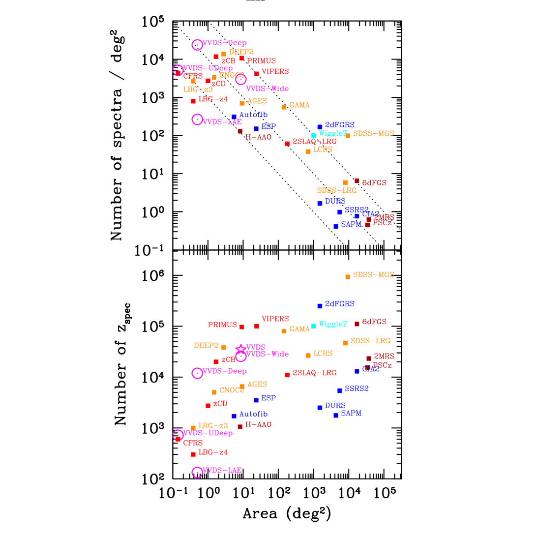
Figure 24: Comparison of the density of spectra (top) and the number of measured spectroscopic redshifts (bottom) versus the observed area, for the VVDS (magenta) and different spectroscopic redshift surveys. The combined VVDS surveys (Wide, deep and Ultra-Deep) are represented by the star symbol (bottom panel). The colour code indicates the wavelength of the sample selection: UV (cyan), B-band (blue), r-band (orange), i-band (red, magenta), IR (brown). zCOSMOS-Bright and zCOSMOS-Deep are labelled ’zCB’ and ’zCD’, respectively. Dashed lines on the top panel represent samples with 1 000, 10 000 and 100 000 redshifts (from bottom to top).

Following Baldry et al. (2010), we have compiled a list of spectroscopic surveys, as listed in Table 5, updated with new and on-going surveys, limiting to spectroscopic samples larger than 100 galaxies. In describing the GAMA survey, Baldry et al. (2010) have compared their survey to other surveys in a plane relating the density of spectra to the area covered by each survey. We present an updated version of this comparison in Figure 24 (top panel), with the VVDS surveys as summarized in this paper. In this plane, the surveys distribution is somewhat bimodal, with larger area surveys with a lower density of spectra on the bottom-right of the plot, and smaller area surveys with a higher density of spectra in the upper-left. All high redshift survey (say beyond $z\sim 0.5$) are of this later category, with the VVDS-Deep presenting the highest density of spectra, followed by the DEEP2 survey. The VVDS-Wide covers an area larger than zCOSMOS-Bright (zCB on the plot) or DEEP2, at a lower spectra density. We show in Figure 24 (bottom panel) the number of spectroscopic redshifts obtained as a function of area for these different surveys. The total number of spectra in the combined VVDS surveys is comparable to the DEEP2 survey, but lower than the number of spectra in the PRIMUS (Coil et al., 2011) and VIPERS surveys limited to $z\sim 1$.

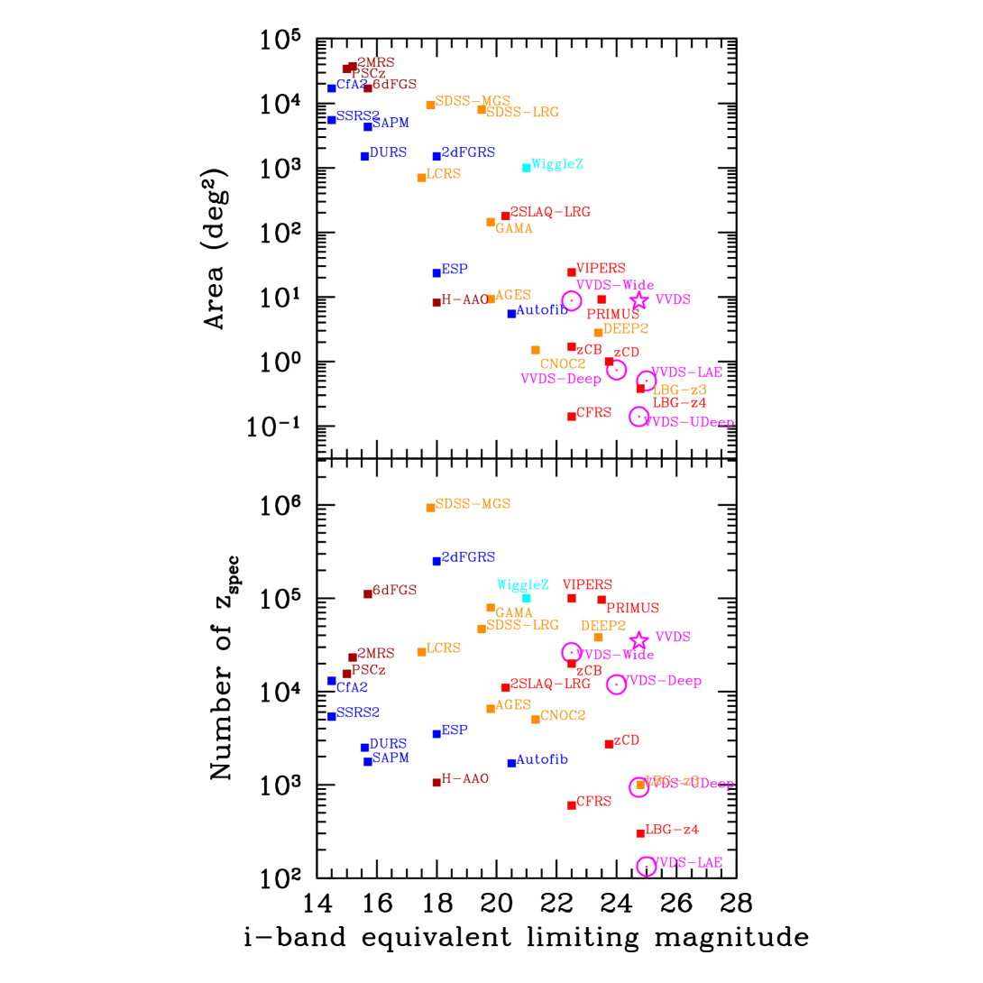
Figure 25: Comparison of the covered area (top) and the number of measured spectroscopic redshifts (bottom) versus depth expressed as the equivalent i–band limiting magnitude, between the VVDS (magenta) and different spectroscopic redshift surveys. The i–band limiting magnitude of each survey has been estimated using the survey band and limiting magnitude in that band, and assuming a flat spectrum. The same colour code as in Figure 24 has been used.

Absent from the two panels in Figure 24 is the key information on the depth and the redshift coverage of each survey. For instance in these plots the VVDS-UltraDeep looks similar to the CFRS as it covers about the same area with the same number density and the same number of spectra, but while the CFRS extends to $z\sim 1.2$ with $i_{AB}\leq 22.5$, the VVDS-UltraDeep extends to $z\sim 4$ with $i_{AB}\leq 24.75$. We therefore compare the number of spectra and covered area versus limiting magnitude in Figure 25. The area (volume) covered by redshift surveys, as well as the number of spectra, are, as expected, getting smaller with increasing limiting magnitude or redshifts. The VVDS-Deep, VVDS-UltraDeep and VVDS-LAE contribute some of the deepest spectroscopic redshift surveys to date.

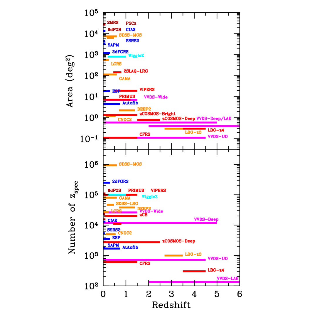
Figure 26: Comparison of the covered area (top) and the number of measured spectroscopic redshifts (bottom) versus redshift, between the VVDS (magenta) and different spectroscopic redshift surveys. The same colour code as in Figure 24 has been used

To give further indications on the useful range of these surveys, we compare in Figure 26 the number of redshifts obtained by the VVDS to other surveys, as well as the area covered, as a function of redshift. The uniqueness of VVDS is evident as the VVDS surveys covers the largest redshift range of all surveys, and reach among the highest redshifts.

Another interesting comparison between surveys is the total time necessary to complete a survey. The observing efficiency of a survey is characterized by the number of (clear) observing nights (hours) necessary to assemble the redshifts. The VVDS-Wide, Deep, and Ultra-Deep surveys took 120h, 160h, and 150h on VIMOS at the VLT, respectively, including all overheads. By comparison at $z\sim 1$, the CFRS took the equivalent of 19 clear nights ($\sim 190$h) on the MOS-SIS at the 3.6m CFHT (Le Fèvre et al 1995) and DEEP2 took 90 nights ($\sim 900$h) on DEIMOS at the 10m Keck telescope (Newman et al. 2012).

As a summary from these comparisons, the complementarity of deep galaxy spectroscopic surveys is evident in the parameter space defined by the number of spectra, area, depth, and redshift coverage. The VVDS survey is providing a unique galaxy sample, selected in magnitude, with the widest redshift coverage of existing surveys and an homogeneous treatment of spectra, and with depth, covered area, and number of spectra comparable to or better than other high redshift spectroscopic surveys existing today.

8 VVDS complete data release

The data produced by the VVDS are all publicly released on a database with open access. A complete information system has been developed with the data embedded in a reliable database environment, as described in Le Brun et al. (in preparation). Queries combining the main survey parameters can be defined on the high–level user interface or through SQL commands. Interactive plotting capabilities enable to identify the galaxies with redshifts on the deep images, and to view all the spectroscopic and photometric information of each object with redshift, including spectra and thumbnails image extractions. Spectra and images can be retreived in FITS format.

The main parameters available on the database are as follows:

• Identification number, following the IAU notation ID-alpha-delta

• $\alpha_{2000},\delta_{2000}$ coordinates

• Broad band photometric magnitudes u’grizJHKs

• Spectroscopic redshift

• Spectroscopic redshift reliability flag

• Photometric redshift

• TSR, SSR, PSR weights

• Spectroscopic and photometric masks (region files)

In addition, specific parameters from connected surveys are available, depending on each of the VVDS fields, including e.g. Galex UV photometry, Spitzer-Swire photometry, VLA radio flux, etc.

The photometric data and spectra of 12 430 Galactic stars are also available on this data release.

All the VVDS data can be queried on http://cesam.lam.fr/vvds.

9 Summary

We have presented the VVDS surveys as completed, including the VVDS-Wide, VVDS-Deep, VVDS-UltraDeep, and VVDS-LAE. In total the VVDS has measured spectroscopic redshifts for 34 594 galaxies and $422$ AGN over a redshift range $0.007\leq z_{spec}\leq 6.62$, over an area up to 8.7 deg², for magnitude-limited surveys with a depth down to $i_{AB}=24.75$ and line flux $F=1.5\times 10^{18}$ erg/s/cm². The VVDS-Wide sample sums up to 25 805 galaxies with $I_{AB}\leq 22.5$ over $0<z<2$, and a mean spectroscopic redshift $\bar{z}=0.55$. The VVDS-Deep contains 11 486 galaxies with $17.5\leq I_{AB}\leq 24.0$ over $0<z<5$ and $\bar{z}=0.92$. The VVDS Ultra-Deep contains 938 galaxies with measured redshifts with $23\leq i_{AB}\leq 24.75$ over $0<z<4.5$ and $\bar{z}=1.38$. The VVDS-LAE sample adds 133 serendipitously discovered LAE to the high redshift populations with $2<z\leq 6.62$.

Independent and deeper observations have been obtained on $\sim 1250$ galaxies, which has enabled to fully assess the reliability of the redshift measurements. A reliability flag is associated to each redshift measurement through inter-comparison of measurements performed independently by two team members. We demonstrate that galaxies with VVDS flags 2, 3, 4 and 9 have a reliability ranging from 83 to 100%, making this the primary sample for science analysis. Galaxies with flag=1 can be used for science analyses after taking into account that they have a $\sim$50% probability to be correct. We emphasize that this probabilistic flag system enables a robust statistical treatment of the survey selection function, compiling a finer information than a simplistic good/bad redshift scheme. This leads to a well described selection function with the TSR (Target Sampling Rate), PSR (Photometric Sampling Rate), and SSR (Spectroscopic Success Rate) which are magnitude and redshift dependent, as characterized in this paper, and available in our final data release.

We have emphasized the dependency of the ’redshift desert’ on instrumental setups, and demonstrated that it can be successfully crossed when using a wavelength domain $3650\leq\lambda\leq 9350$Å. This wavelength range allows to follow the main emission/absorption tracers like [OII]3727 or CaH&K which would leave the domain for $z\geq 1.5$, while CIV-1549Å and Ly$\alpha$-1215Å would enter the domain for $z\geq 1.32$ and $z\geq 2$ respectively.

The basic properties of the VVDS samples have been described, including the apparent and absolute magnitude distributions, as well as the ($M_{u}-M_{r}$, $M_{r}$) colour-magnitude distribution showing a well defined colour bi-modality starting to be prominent at $1\leq z\leq 1.5$, with a red sequence present up to $z\sim 2$. Averages of the observed VVDS-Deep and VVDS-UltraDeep spectra have been produced in redshift bins covering $0<z<5$.

The comparison of the VVDS survey with other spectroscopic redshift surveys shows the unique place of the VVDS in the parameter space defined by the number of spectra, area, depth, and redshift coverage, complementary to other surveys at similar redshifts.

All the VVDS data in this final release are made publicly available on a dedicated database available at http://cesam.lam.fr/vvds.

Table 5: Comparison of VVDS surveys with other spectroscopic redshift surveys, by order of increasing mean redshift (updated from Baldry et al. 2010)

$$\begin{array}[]{lrlrclll}\hline\cr\hline\cr\vskip 3.0pt plus 1.0pt minus 1.0pt\cr Survey&Area&Depth\leavevmode\nobreak\ i_{AB}^{a}&N_{obj}&z_{range}&z_{mean}&Selection&Reference\\ \vskip 3.0pt plus 1.0pt minus 1.0pt\cr\hline\cr\vskip 3.0pt plus 1.0pt minus 1.0pt\cr SSRS2&5500&14.5&5\,369&0.0-0.08&0.03&B<15.5&$da Costa et al. 1998$\\ PSCz&34000&15.0&15\,411&0.0-0.1&0.03&60\mu_{AB}<9.5&$Saunders et al. 2000$\\ 2MRS&37000&15.2&23\,200&0.0-0.08&0.03&K<15.2&$Erdo\u{g}du et al. 2006$\\ SAPM&4300&15.7&1\,769&0.0-0.1&0.034&BJ<17.1&$Loveday et al. 1992$\\ 6dFGS&17000&15.7&110\,256&0.0-0.1&0.05&K<12.7&$Jones et al. 2009$\\ CfA2&17000&14.5&13\,000&0.0-0.1&0.05&B<15.5&$Falco et al. 1999$\\ DURS&1500&15.6&2\,500&0.0-0.2&0.07&BJ<17.0&$Ratcliffe et al. 1996$\\ LCRS&700&17.5&26\,418&0.0-0.25&0.1&R<17.5&$Shectman et al. 1996$\\ 2dFGRS&1500&18.0&250\,000&0.0-0.3&0.11&BJ<19.4&$Colless et al. 2001$\\ H-AAO&8.2&18.0&1\,056&0.0-0.55&0.14&KAB<16.8&$Huang et al. 2003$\\ ESP&23.3&18.0&3\,500&0.0-0.3&0.15&BJ<19.4&$Vettolani et al. 1997$\\ AGES&9.3&19.8&6\,500&0.0-0.5&0.2&R<20B_{W}<20.5&$Watson et al. 2009$\\ GAMA&144&19.8&79\,599&0.0-0.6&0.25&r<19.8,z<18.2,K_{AB}<17.6&$Baldry et al. 2010$\\ CNOC2&1.5&21.3&5\,000&0.12-0.55&0.3&R<21.5&$Yee et al. 2000$\\ Autofib&5.5&20.5&1\,700&0.0-0.75&0.3&B_{J}<22&$Ellis et al. 1996$\\ SDSS-LRG&8000&19.5&46\,748&0.16-0.47&0.3&r<19.5+CS^{b}&$Eisenstein et al. 2005$\\ SDSS-MGS&9380&17.8&935\,000&0.0-0.6&0.3&r<17.8,DR7&$Abazajian et al. 2009$\\ 2SLAQ-LRG&180&20.3&11\,000&0.45-0.8&0.5&i<19.8+CS&$Cannon et al. 2006$\\ CFRS&0.14&22.5&600&0-1.5&0.55&I_{AB}\leq 22.5&$Lilly et al. 1995$\\ zCosmos-Bright&1.7&22.5&20\,000&0-1.5&0.55&17.5\leq i_{AB}\leq 22.5&$Lilly et al. 2007$\\ {\bf VVDS-Wide}^{c}&8.7&22.5&26\,178&0-1.5&0.55&17.5\leq I_{AB}\leq 22.5&$Garilli et al. 2008$\\ PRIMUS&9.1&23.5&96\,599&0.0-1.2&0.6&i_{AB}\leq 23&$Coil et al. 2011$\\ WiggleZ&1000&21.0&100\,000&0.2-1.0&0.6&NUV<22.8+CS&$Blake et al. 2011$\\ {\bf VVDS-Deep}&0.74&24.00&11\,601&0-5&0.92&17.5\leq I_{AB}\leq 24.0&$Le F\`{e}vre et al. 2005a, this paper$\\ DEEP2&2.8&23.4&38\,000&0.7-1.4&1.0&RAB<24.1+CS&$Newman et al. 2012$\\ VIPERS&24&22.5&100\,000&0.5-1.5&1.0&17.5\leq i_{AB}\leq 22.5+CS&$Guzzo et al. 2013$\\ {\bf VVDS-UDeep}&0.14&24.75&941&0-4.5&1.38&23.0\leq i_{AB}\leq 24.75&$This paper$\\ zCosmos-Deep&1&23.75&2\,728&1.5-2.5&2.1&B_{AB}\leq 25+CS&$Lilly et al. 2007$\\ LBG-z3&0.38&24.8&1\,000&2.7-3.5&3.2&R_{AB}<25.5+CS&$Steidel et al. 2003$\\ VUDS&1&25&10\,000&2-6.7&3.7&i_{AB}<25+photo-z&$Le F\`{e}vre et al., in prep.$\\ LBG-z4&0.38&25.0&300&3.5-4.5&4.0&I_{AB}<25+CS&$Steidel et al. 1999$\\ \vskip 3.0pt plus 1.0pt minus 1.0pt\cr\hline\cr\vskip 3.0pt plus 1.0pt minus 1.0pt\cr{\bf VVDS-All}^{d}&8.7&24.75&35\,016&0-5&1.2&$Combined VVDS$&$This paper$\\ \vskip 3.0pt plus 1.0pt minus 1.0pt\cr\hline\cr\end{array}$$

• Equivalent depth in $i_{AB}$ using a flat spectrum transformation from the original survey depth.

• CS: Colour Selection, varies from survey to survey

• The VVDS-Wide includes all objects with $17.5\leq I_{AB}\leq 22.5$ in all 5 VVDS fields

• Includes all objects in the 3 VVDS-Wide fields (1003+01, 1400+05 and 2217+00), in the VVDS-Deep fields (0226 and ECDFS), in the VVDS-UltraDeep field (0226-04), and the LAE emitters, as described in Table 1

References

- (1) Abazajian et al., 2009, ApJS, 182, 543
- (2) Abraham, R., et al., 2004, AJ, 127, 2455
- (3) Arnouts, S., et al., 2005, ApJ, 619, 43
- (4) Arnouts, S., et al., 2007, A&A, 476, 137
- (5) Baldry, I., et al., 2010, MNRAS, 404, 86
- (6) Bertin, E., Arnouts, S., 1996, A&AS, 117, 393
- (7) Bielby, R., et al., 2012, A&A, 545, 23
- Blake et al. (2011) Blake, C., et al., 2011, MNRAS, 418, 1707
- (9) Bondi, M., et al., 2003, A&A, 403, 857
- (10) Bottini, D., et al., 2005, PASP, 117, 996
- Cannon et al. (2006) Cannon, R., et al., 2006, MNRAS, 372, 425
- (12) Cassata, P., Le Fèvre, O., et al., 2011, A&A, 525, 143
- (13) Cassata, P., Le Fèvre, O., et al., 2013, A&A, 556, 68
- (14) Cimatti, A., et al., 2008, A&A, 482, 21
- Coil et al. (2011) Coil, A., et al., 2011, ApJ, 741, 8
- Colless et al. (1990) Colless, M., Ellis, R.S., Taylor, K., Hook, R.N., 1990, MNRAS, 244, 408
- Colless et al. (2001) Colless, M., et al., 2001, MNRAS, 328, 1039
- Conti et al. (2001) Conti, G., et al., 2001, PASP, 113, 452
- Contini et al. (2012) Contini, T., et al., 2012, A&A, 539, 91
- Cucciati et al. (2012) Cucciati, O., et al., 2012, A&A, 539, 31
- Cucciati et al. (2010) Cucciati, O., et al., 2010, A&A, 520A, 42
- Cucciati et al. (2006) Cucciati, O., et al., 2006, A&A, 458, 39
- Cuillandre et al. (2012) Cuillandre, J.C., et al., 2012, Proc. SPIE 8448, Observatory Operations: Strategies, Processes, and Systems IV, 84480
- (24) da Costa, L., et al., 1998, AJ, 116, 1
- (25) Daddi, E., et al., 2004, ApJ, 617, 746
- Davis et al., (2003) Davis, M., et al., 2003, SPIE, 4834, 161
- de la Torre et al., (2011) de la Torre, S., et al., 2011, A&A, 525, 125
- de Ravel et al., (2009) de Ravel, L., et al., 2009, A&A, 498, 379
- Erdogdu et al. (2006) Erdoğdu, P. et al., 2006, MNRAS, 373, 45
- Eisenstein et al. (2005) Eisenstein et al., 2005, ApJ, 633, 560
- Ellis et al. (1996) Ellis, R.S., et al. 1996, MNRAS, 280, 235
- Epinat et al. (2009) Epinat, B., et al., 2009, A&A, 504, 789
- Falco et al. (1999) Falco, E., et al.,1999, PASP, 111, 438
- (34) Forster-Schreiber, N., et al., 2009, ApJ, 706, 1364
- Franzetti et al. (2007) Franzetti, P., et al., 2007, A&A, 465, 711
- Garilli et al. (2008) Garilli, B., et al., 2008, A&A, 486, 683
- Garilli et al. (2010) Garilli, B., et al., 2010, PASP, 122, 827
- Guzzo et al. (2008) Guzzo, L., et al., 2008, Nature, 451, 541
- Guzzo et al. (2013) Guzzo, L., et al., 2013, arXiv:1303.2623
- Hook et al. (2003) Hook, I., et al., 2003, SPIE, 4841, 1645
- Huang et al. (2003) Huang et al. 2003, ApJ, 584, 203
- Ilbert et al. (2005) Ilbert, O., et al., 2005, A&A, 439, 863
- Ilbert et al. (2006) Ilbert, O., et al., 2006, A&A, 457, 841
- Ilbert et al. (2009) Ilbert, O., et al., 2009, ApJ, 690, 1236
- Iovino et al. (2005) Iovino, A., et al., 2005, A&A, 442, 423
- Jones et al. (2009) Jones, D.H., et al., 2009, MNRAS, 399, 683
- Law et al. (2009) Law, D., et al., 2009, ApJ, 697, 2057
- Lawrence et al. (2007) Lawrence, A. et al., 2007, MNRAS, 379, 1599
- Le Fèvre et al. (1994) Le Fèvre, O., Crampton, D., Felenbok, P., Monnet, G., 1994, A&A, 282, 325
- Le Fèvre et al. (1995) Le Fèvre, O., Crampton, D., Lilly, S.J., Hammer, F., Tresse, L., 1995, ApJ, 455, 60
- Le Fèvre et al. (2003) Le Fèvre, O., et al., 2003, SPIE, 4841, 1670
- Le Fèvre et al. (2004a) Le Fèvre, O., et al., 2004a, A&A, 428, 1043
- Le Fèvre et al. (2004b) Le Fèvre, O., et al., 2004b, A&A, 417, 839
- Le Fèvre et al. (2005a) Le Fèvre, O., et al., 2005a, A&A, 439, 845
- Le Fèvre et al. (2005b) Le Fèvre, O., et al., 2005b, Nature, 437, 519
- Le Fèvre et al. (2013) Le Fèvre, O., et al., 2013, A&A, arXiv:1307.6518
- Lemoine-Busserolle et al. (2010) Lemoine-Busserolle, M., Bunker, A., Lamareille, F., Kissler-Patig, M., 2010, MNRAS, 401, 1657
- Lilly et al. (1991) Lilly, S.J., Cowie, L.L., Gardner, J.P., 2001, ApJ, 369, 79
- Lilly et al. (1995) Lilly, S.J., Le Fèvre, O., Crampton, D., Hammer, F., 1995a, ApJ, 455, 50
- Lilly et al. (1996) Lilly, S. J., Le Fèvre, O., Hammer, F., Crampton, D., 1996, ApJ, 460, 1
- Lilly et al. (2007) Lilly, S.J., Le Fèvre, O., et al., 2007, ApJS, 172, 70
- (62) Lonsdale, C.C., et al., 2003, PASP, 115, 897
- (63) López-Sanjuan, C., et al., 2011, A&A, 530, 20
- Loveday et al. (1992) Loveday, J., et al., 1992, ApJ, 390,338
- Madau et al. (1996) Madau, P., Ferguson, H.C., Dickinson, M., Giavalisco, M., Steidel, C.C., Fruchter, A., 1996, MNRAS, 283, 1388
- McCracken et al. (2003) McCracken, H. J., Radovich, M., Bertin, E., Mellier, Y., Dantel-Fort, M., Le Fèvre, O., Cuillandre, J. C., Gwyn, S., Foucaud, S., Zamorani, G., 2003, A&A, 410,17
- Meneux et al. (2009) Meneux, B., et al., 2009, A&A, 505, 463
- Newman et al. (2012) Newman, J., et al., 2012, arXiv:1203.3192
- Noll et al. (2004) Noll, S., et al., 2004, A&A, 418, 885
- Oliver et al. (2012) Oliver, S., et al., 2012, MNRAS, 424, 1614
- Ouchi et al. (2010) Ouchi, M., et al., 2010, ApJ, 723, 869
- (72) Pierre, M., et al., 2004, JCAP, 09, 011
- Popesso et al. (2009) Popesso, et al., 2009, A&A, 494, 443
- Pozzetti et al. (2007) Pozzetti, L., A&A, 474, 443
- Radovich et al. (2004) Radovich, M., et al., 2004, A&A, 417, 51
- Ratcliffe et al. (1996) Ratcliffe et al. 1996, MNRAS, 281, 47
- Saunders et al. (2000) Saunders et al. 2000, MNRAS, 317, 55
- Shectman et al. (1996) Shectman, S.A., et al. 1996, ApJ, 470, 172
- (79) Scodeggio, M., et al., 2005, PASP, 117, 1284
- Scoville et al. (2007) Scoville, N., et al., 2007, ApJS, 172, 1
- Steidel et al. (1996) Steidel, C.C., Giavalisco, M., Pettini, M., Dickinson, M., Adelberger, K.L., 1996, ApJ, 462, 17
- Steidel et al. (1999) Steidel, C.C., Adelberger, K.L., Giavalisco, M., Dickinson, M., Pettini, M., 1999, ApJ, 519, 1
- (83) Steidel, C.C., et al., 2003, ApJ, 592, 728
- Temporin et al. (2008) Temporin, S., et al., 2008, A&A, 482, 81
- (85) Tresse, L., et al., 2007, A&A, 472, 403
- Vettolani et al. (1997) Vettolani, G., et al. 1997, A&A, 325, 954
- Watson et al. (2009) Watson, M.G., et al. 2009, A&A, 493, 339
- Yee et al. (2000) Yee et al. 2000, ApJS, 129, 475
- (89) York, D.G., et al., 2000, AJ, 120, 1579
- (90) Zucca, E., et al., 2006, A&A, 455, 879