An Experimental Comparison of Speed Scaling Algorithms with Deadline Feasibility Constraints

Abstract

We consider the first, and most well studied, speed scaling problem in the algorithmic literature: where the scheduling quality of service measure is a deadline feasibility constraint, and where the power objective is to minimize the total energy used. Four online algorithms for this problem have been proposed in the algorithmic literature. Based on the best upper bound that can be proved on the competitive ratio, the ranking of the online algorithms from best to worst is: ${\rm qOA}$, ${\rm OA}$, ${\rm AVR}$, ${\rm BKP}$. As a test case on the effectiveness of competitive analysis to predict the best online algorithm, we report on an experimental “horse race” between these algorithms using instances based on web server traces. Our main conclusion is that the ranking of our algorithms based on their performance in our experiments is identical to the order predicted by competitive analysis. This ranking holds over a large range of possible power functions, and even if the power objective is temperature.

1 Introduction

Energy consumption has become a key issue in the design of microprocessors. Major chip manufacturers, such as Intel, AMD and IBM, now produce chips with dynamically scalable speeds, and produce associated software, such as Intel’s SpeedStep and AMD’s PowerNow, that enables an operating system to manage power by scaling processor speed. Thus the operating system should have an online speed scaling policy for setting the speed of the processor, that ideally should work in tandem with a job selection policy for determining which job to run. In order to be implementable in a real system, these policies must be online since the system will not in general be aware of which jobs will arrive in the future.

The resulting online optimization problems, generally called speed scaling problems, have dual objectives as one both wants to optimize some schedule quality of service objective and some power related objective. In this paper we consider the first [10], and most well studied [10, 2, 6, 5, 4, 9, 8, 1, 7], speed scaling problem in the algorithmic literature: where the scheduling quality of service measure is a deadline feasibility constraint (each job must be completed by its deadline), and where the power objective is to minimize the total energy used.

This problem can be more formally described as follows. A problem instance consists of $n$ tasks. Task $i$ has a release time $r_{i}$, a deadline $d_{i}>r_{i}$, and work $w_{i}>0$. An online scheduler learns about a task only at its release time; at this time, the scheduler also learns the exact work requirement and the deadline of the task. A schedule specifies for each time a task to be run and a speed at which to run the task. The speed is the amount of work performed on the task per unit time. Thus, a task with work $w$ run at a constant speed $s$ takes time $\frac{w}{s}$ to complete. More generally, the work done on a task during a time period is the integral over that time period of the speed at which the task is run. A schedule is feasible if for each task $i$, work at least $w_{i}$ is done on task $i$ during $[r_{i},d_{i}]$. Note that the times at which work is performed on task $i$ do not have to be contiguous. Essentially all of the algorithmic literature has assumed a power function, which specifies the power $P$ usage as a function of the speed $s$ of the processor, as $P=s^{\alpha}$, where $\alpha>1$ is some constant. Of particular interest is $\alpha=3$ since dynamic power in CMOS based processors is approximately the speed cubed. The energy used during a time period is the integral of the power over that time period.

It is easy to see that without loss of generality one can adopt Earliest Deadline First (${\rm EDF}$) as the job selection algorithm. So the problem reduces to finding algorithms for speed scaling. Four online speed scaling algorithms for this problem has been proposed in the literature. Table 1 summarizes where each of these algorithms were proposed, and the best known bounds on the competitive ratio for these algorithms. We now briefly describe these algorithms:

Average Rate (${\rm AVR}$) runs each job at a constant speed between its release and its deadline. The attraction of the algorithm ${\rm AVR}$ is that it is in some sense fair to all jobs.

Optimal Available (${\rm OA}$) runs at the speed that would be optimal, given the current state, and given that no more tasks will arrive. This speed can be determined using the offline greedy algorithm ${\rm YDS}$ from [10] for computing an optimal schedule.

${\rm BKP}$ intuitively computes the least possible speed that optimal offline schedule ${\rm YDS}$ might currently be running at given the tasks that have arrived to date, and then runs at $e$ times that speed. (If the algorithm ran at some constant $q<e$ times this lower bound, the deadline of some jobs may be missed.)

${\rm qOA}$ runs at speed equal to some constant $q\geq 1$ times the speed that ${\rm OA}$ would run in the current state.

Algorithm	General $\alpha$
	Upper	Lower
General		$e^{\alpha-1}/\alpha\cite[cite]{[\@@bibref{}{qOA}{}{}]}$
AVR[10]	$2^{\alpha-1}\alpha^{\alpha}$[10, 2]	$(2-\delta)^{\alpha-1}\alpha^{\alpha}$[2]
OA[10]	$\alpha^{\alpha}$[4]	$\alpha^{\alpha}$[10]
BKP[4]	$2(\alpha/(\alpha-1))^{\alpha}e^{\alpha}$[4]
qOA[3]	$4^{\alpha}/(2\sqrt{e\alpha})$[3]	$\frac{1}{2q\alpha}4^{\alpha}(1-\frac{2}{\alpha})^{\alpha/2}$[3]
	when $q=2-\frac{1}{\alpha}$
	$\alpha=3$
	Upper	Lower
General		2.4
AVR	108	48
OA	27	27
BKP	135.6
qOA	6.7
	when $q=1.54$

Table 1: Where the online algorithms in the literature were proposed, and the best known bounds on the competitive ratios

Competitive analysis for online scheduling problems in particular, and online problems in general, is sometimes criticized for a variety of reasons. The most common criticism is that competitive analysis focuses on worst-case performance, and thus may not predict the algorithm that performs best in practice, or on average. However, competitive analysis likely will not go away because it can be tractably applied to such a wide range of problems, for which it is not clear how to obtain a useful average case analysis. Competitive analysis has applied to several reasonable algorithms for this problem, and the search for optimally competitive algorithms has lead to candidate algorithms that would not likely have been discovered by local search and experimentation. Plausibly any of these candidate algorithms might be the best experimentally.

So as a test case on the effectiveness of competitive analysis to predict the best experimental online algorithm, we report on an experimental “horse race” between these speed scaling algorithms. Our data was based on web traces, which naturally gave release times and sizes for each job. We consider several natural ways of adding deadlines to the jobs, and tweak the data to produce inputs with workloads with different levels of spikiness. Based on the best upper bound that can be proved on the competitive ratio, when $\alpha$ is around 3, the ranking of the online algorithms from best to worst is: ${\rm qOA}$, ${\rm OA}$, ${\rm AVR}$, ${\rm BKP}$. Our experimental results are essentially that over the wide range of input instances we tried, the order of the algorithms from best to worst was exactly the same order as predicted by the best known upper bounds on the competitive ratio. Further, the differences between the various algorithms was significant. So these experimental results can be viewed as a victory for competitive analysis (or alternatively as a defeat for critics of competitive analysis).

A priori we intuitively expected ${\rm BKP}$ to be the best experimental algorithm, not the worst. We believed that the reason that the best known competitive ratio for ${\rm BKP}$ was so high was that its non-local nature made it more difficult to analyze accurately. To understand the conceptual difference between ${\rm BKP}$ and ${\rm qOA}$, consider a situation where the current load (unfinished work) is low, but the load in the recent past was high. In this situation ${\rm BKP}$ may run at a high speed, while ${\rm qOA}$ definitely will not run at a high speed. It seemed to us that ${\rm BKP}$’s use of the historical load should give it an advantage. Further, in the extreme, when $\alpha=\infty$, the energy optimal schedule is one that is optimal with respect to the maximum speed that it reaches. [4] show that ${\rm BKP}$ is optimally $e$-competitive with respect to maximum speed. This led us to believe that ${\rm BKP}$ is near optimally competitive for large $\alpha$. Further, there appears to be no obvious reason why the relative performance of the algorithms should depend on $\alpha$. Thus, we expected that ${\rm BKP}$ would also be the best algorithm when the cube-root rule ($\alpha=3$) holds.

Some other experimental observations that we believe are interesting are:

• The performance of ${\rm qOA}$ is not so sensitive to the value of $q$. Picking $q$ to be in the range $[1.5,2]$, as suggested by the competitiveness results, gives performance reasonably close to the optimal $q$ for each particular instance. We select $q=1.5$ in comparison with other algorithms because this is the value of $q$ suggested by the competitive analysis of ${\rm qOA}$.

• The schedule produced by ${\rm qOA}$ uses less energy than the schedules produced by ${\rm AVR}$ or ${\rm BKP}$.

• There are two alternative formulations of the algorithm ${\rm BKP}$ given in [4]. We find that the one that produces a better (higher) lower bound for the speed of the optimal algorithm ${\rm YDS}$ at the current time, is the worse performing of the two alternatives.

• The value of $q$ is generally higher for moderately spiky workloads than for flat ones. For flat and moderately spiky workloads, the optimal $q$ for the ${\rm qOA}$ algorithm is usually high— typically around 4 or higher. This is significant because it shows that ${\rm BKP}$ loses to ${\rm qOA}$ even when the multiplier $q$ is relatively large (and bigger than the multiplier $e$ used in ${\rm BKP}$). Intuitively this suggests that the main reason that ${\rm BKP}$ loses relative to ${\rm qOA}$ is because of its consideration of load in the recent past. Further, for these workloads, the optimal value of $q$ tends to increase as $\alpha$ is increased.

• For highly spiky workloads and workloads with a fixed time span for all jobs, the optimal value of $q$ for ${\rm qOA}$ is quite low— near 1. This is true for fixed time span workloads regardless of the length of the fixed time span. For these workloads, the optimal value of $q$ usually decreases as $\alpha$ is increased.

• [4] also showed that ${\rm BKP}$ and ${\rm YDS}$ are cooling oblivious, i.e. they are simultaneously constant-competitive with respect to temperature for all values of the cooling parameter assuming that the environment has a fixed ambient temperature and that the device cools according to Newton’s law of cooling. This led us to also compare the various algorithms with respect to the objective of maximum temperature. The relative ordering of the algorithms with respect to maximum temperature is the same as their order with respect to energy consumption. Further, the energy optimal schedule ${\rm YDS}$ is better than ${\rm qOA}$ with respect to maximum temperature.

All of the implementations of the speed scaling algorithms, and related programs, such as those for generating test instances, can be found at http://www.cs.pitt.edu/$\sim$kirk/SpeedScalingExperiments. We expect, or at least hope, that these tools will be useful to future researchers.

It is important to note again that the purpose of this paper was to determine how the performance of the candidate algorithms predicted by competitive analysis compared to a generic experimental analysis. Thus we based our input on web traces instead of program traces because these were more readily available, and still served our purposes. We acknowledge that the common abstract model for a processor, which we use in this paper, is a significant simplification of a real processor, and that there are many significant issues that would have to be addressed in applying these algorithms in a real setting. But these lower level implementation issues are beyond the scope of this paper.

The rest of the paper is organized as follows. In section 2 we give more formal definitions of the problem and algorithms. In section 3 we explain our experimental setup. In section 4 we give our experimental observations.

2 Preliminaries

Newton’s Law of heat conduction states that the rate of cooling is proportional to the difference in temperature between the object and its environment. We assume the environment has a fixed temperature and that temperature is scaled so that the environmental temperature is zero. A first-order approximation for the rate of change $T^{\prime}$ of the temperature $T$ is then $T^{\prime}=P-bT$, where $P$ is the power used at time $t$, and $b$ is a constant.

A schedule is $R$-competitive, or $R$-approximate, for a particular objective function if the value of that objective function on the schedule is at most $R$ times the value of the objective function on an optimal schedule. An algorithm $A$ is $R$-competitive, or has competitive ratio $R$, if $A(I)$ is $R$-competitive for all instances.

We now more formally define the algorithms that we consider in this paper, along with related concepts. The span of a job $i$ is $d_{i}-r_{i}$. We start with the offline speed scaling algorithm ${\rm YDS}$ proposed in [10]. Let $w(t_{1},t_{2})$ denote the work that has release time at least $t_{1}$ and has deadline at most $t_{2}$. The intensity $I(t_{1},t_{2})$ of the time interval $[t_{1},t_{2}]$ is defined to be $w(t_{1},t_{2})/(t_{2}-t_{1})$.

Algorithm ${\rm YDS}$ [10]: The algorithm repeats the following steps until all jobs are scheduled:

1. Let $[t_{1},t_{2}]$ be the maximum intensity time interval.

2. The processor will run at speed $I(t_{1},t_{2})$ during $[t_{1},t_{2}]$ and schedule all the jobs comprising $w(t_{1},t_{2})$, always running the released, unfinished task with the earliest deadline.

3. Then the instance is modified as if the times $[t_{1},t_{2}]$ didn’t exist. That is, all deadlines $d_{i}>t_{1}$ are reduced to $\max(t_{1},d_{i}-(t_{2}-t_{1}))$, and all release times $r_{i}>t_{1}$ are reduced to $\max(t_{1},r_{i}-(t_{2}-t_{1}))$.

Algorithm ${\rm qOA}$ [3]: The speed is $q\cdot\max_{t}w(t)/t$, where $w(t)$ is the unfinished work that has deadline within the next $t$ units of time. Here $q$ is some constant that is at least 1. We set $q=1.5$ when we compare ${\rm qOA}$ to other algorithms. ${\rm OA}$ is just the algorithm ${\rm qOA}$ when $q=1$.

Algorithm ${\rm AVR}$ [10]: The speed is $\sum_{i\in J(t)}\frac{w_{i}}{d_{i}-r_{i}}$, where $J(t)$ is the collection of tasks $i$ with $r_{i}\leq t\leq d_{i}$.

Algorithm ${\rm BKP}$ [4]: For $t_{1}\leq t\leq t_{2}$, let $w(t,t_{1},t_{2})$ denote the amount of work that has release time at least $t_{1}$ and deadline at most $t_{2}$ and that has already arrived by time $t$. Let $p(t)$ be defined by:

$$p(t)=\max_{t_{1},t_{2}}\frac{w(t,t_{1},t_{2})}{(t_{2}-t_{1})}\qquad\textrm{ such that $t_{1}<t\leq t_{2}$}$$

Let $v(t)$ be defined by:

$$v(t)=\max_{t^{\prime}>t}\frac{w(t,et-(e-1)t^{\prime},t^{\prime})}{e(t^{\prime}-t)}$$

In one variation of ${\rm BKP}$ in [4], the speed is $e\cdot v(t)$, and in the other variation, it is $e\cdot p(t)$. Note that $w(t,t_{1},t_{2})$, $p(t)$ and $v(t)$ may be computed by an online algorithm at time $t$. It is easy to see that $v(t)\leq p(t)$.

3 Experimental Setup

We use the trace file epa-http.txt from the Internet Traffic Archive (http://ita.ee.lbl.gov/) to generate the workloads for our experiments. This trace contains about 50,000 http requests received during one day by the EPA’s webserver located at Research Triangle Park, NC. Each http request has two main pieces of information: its time and the number of bytes in the response. Some requests received 0 bytes in response, nearly always corresponding to a 304 (page not modified since last download) or 404 (page not found) response code. In these cases, we treat the response size as 50 bytes to approximate the header; this value is small relative to the responses generated by other requests. We treat each http request as a job whose release time is the same as the http request time, whose work requirement is the number of transferred bytes in response to the request, and whose deadline is generated in different ways to produce workloads with specific characteristics.

Since our trace file contains a day’s worth of http requests, it has a peak period and slow periods corresponding to high traffic and low traffic reaching the website, respectively. Since we are interested in workloads with different degrees of spikiness, we repeat the set of jobs we create based on the trace file five times to simulate having requests of five days.

To allow us to run multiple experiments on this one trace, in each experiment we only create a job for every 20${}^{\textrm{th}}$ http request in the original trace. This allows us to generate 20 different workloads where the first one starts with the first http request in the file, the second workload starts with the second http request, and so on. Each of these workloads contains different jobs, but each spans the entire day and contains similar variations in request density. In addition to providing multiple input workloads, splitting the trace this way also keeps the computation time of our simulator reasonable. In our simulations, the results of the different workloads exhibited similar trends, so we arbitrarily chose the workload generated starting with the sixth job to present its simulation results.

We will now explain how the deadline is generated for each type of workload. Through these explanations the variable $S$ will stand for a fixed scaling factor, and $N$ will denote some random number. We start with the flat and fixed span workloads. These are the most natural since they correspond to requiring a response time proportional to the request size, and requiring a fixed response time for every request, respectively. After that, we consider the moderately and highly spiky workloads. We include them because we wanted to compare the algorithms on spikier workloads.

3.0.1 Flat Workload

The first workload we consider is the flat workload, in which the span of each job is proportional to its amount of work. Although the amount of work varies over time in this workload, it does not particularly strain the processor. We call this work load flat because the optimal energy schedule shows a relatively modest number and degree of speed changes. See Figure 1, which is typical of optimal schedules for this type of workload.

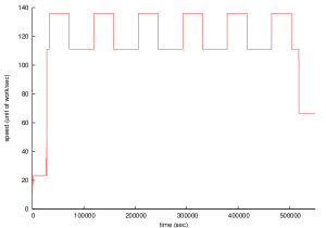
Figure 1: Plot of ${\rm YDS}$ schedule for the flat workload.

We generate the deadlines of jobs in a flat workload using the equation $d_{i}=r_{i}+Sw_{i}$, with $S=0.4$.

3.0.2 Fixed Span Workload

Our second workload is the fixed span workload, in which all jobs have the same span, corresponding to a system that guarantees a worst-case response time for each task. Since jobs vary in their work requirement, the amount of work per unit time varies. The optimal schedule produced by ${\rm YDS}$ for this kind of workload may have large or small variations in speed depending on the job span and how much jobs overlap. Figure 2 plots the ${\rm YDS}$ schedule for one of these workloads generated using a fixed span of 1000 seconds.

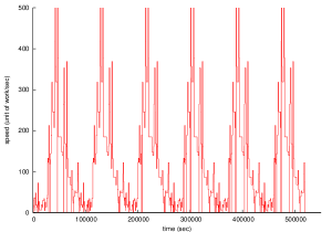
Figure 2: Plot of ${\rm YDS}$ schedule for the fixed span workload.

3.0.3 Moderately Spiky Workload

Our third workload is the moderately spiky workload, which has greater variation in the amount of arriving work. An optimal solution for a moderately spiky workload is shown in Figure 3. To generate the deadlines for this workload, we used the equation $d_{i}=r_{i}+Sw_{i}$, with $S=0.1$. Note that this is the same equation we used to generate a flat workload except for the scaling factor. The change in the optimal schedule can be seen by comparing Figures 1 and 3.

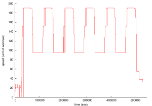
Figure 3: Plot of ${\rm YDS}$ schedule for the moderately spiky workload.

3.0.4 Highly Spiky Workload

For our last workload, which we call the highly spiky workload, we further increased the variability of the amount of work arriving. Intuitively, a highly spiky workload contains bursts of high work when several jobs arrive requiring a lot of work that needs to be finished in a small time period. Therefore, a highly spiky workload contains huge variations in speeds as illustrated by the optimal ${\rm YDS}$ schedule shown in Figure 4.

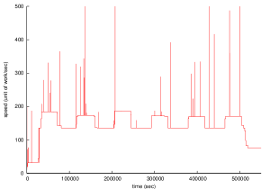
Figure 4: Plot of ${\rm YDS}$ schedule for the highly spiky workload.

When generating this workload, we added additional jobs as well as generating job deadlines. We did this as follows:

1. We divide the time line into intervals of two alternating lengths, $L,H$, with $L>H$. $L$ and $H$ stand for light and high load intervals, respectively. We used $L=200$ and $H=50$.

2. For any job, regardless of whether its release time falls in an $L$ or $H$ interval, we compute its deadline using the equation: $d_{i}=r_{i}+Sw_{i}$, with $S=0.4$.

3. For a job whose release time falls in an $H$ interval we also create zero to two additional jobs with the same release time and amount of work. To compute their deadlines, we first compute the span of the original job (after computing its deadline in the previous step) as $t_{i}=d_{i}-r_{i}$. Then we use the following equation for computing the deadline of each additional job: $d_{i}=r_{i}+Nt_{i}$, where $N$ is a pseudorandom number selected uniformly over the range $(0,2]$. To decide how many additional jobs to create, we use a triangle shaped function $f$ over the high load interval with peak $=2$, and we compute the value $f(x)$ at $x=r_{i}$, the release time of the job; the number of jobs we generate is then $\lceil f(r_{i})\rceil$.

Note that we use a random number in computing the deadlines of these jobs so that we do not have multiple identical jobs which would be equivalent to just one job with the same release time and deadline and an amount of work equal to the sum of their work.

4 Experimental Results

In this section we show the experimental results for the different types of workloads.

Our first observation addresses one possible concern with using ${\rm qOA}$: how does one pick a good value of $q$? For each experiment we run ${\rm qOA}$ with different values of $q$ to find the value that results in the least amount of consumed energy. We tried values of $q$ from $1$ to $9$, increasing in steps of $0.1$. It turns out that the performance of ${\rm qOA}$ is not highly sensitive to the exact value of $q$. Figures 5 and 6 show the consumed energy as a function of $q$ for $\alpha=3$ for the flat and highly spiky workloads, respectively. The curve for a moderately spiky workload is similar to Figure 5, though less steep to the right of the minimum. The curve for a fixed time workload is similar to Figure 6, but with the minimum at 1. In all cases, the curves are relatively flat near the optimal value of $q$, implying that any value near the optimal $q$ produces a near optimal schedule. We set $q=1.5$ when comparing ${\rm qOA}$ to other algorithms because this is the value of $q$ recommended by the competitive analysis of ${\rm qOA}$ when $\alpha$ is about three.

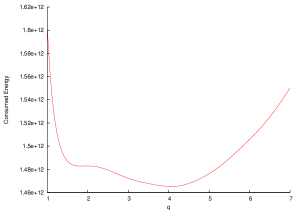
Figure 5: Plot of consumed energy vs. $q$ for ${\rm qOA}$ schedules of a flat workload. ($\alpha=3$)

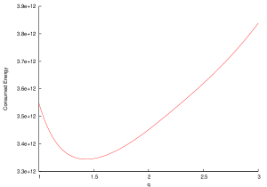
Figure 6: Plot of consumed energy vs. $q$ for ${\rm qOA}$ schedules of a highly spiky workload. ($\alpha=3$)

Now that the choice of $q$ has been addressed, we can compare the different algorithms. In our experiments, the schedule produced by ${\rm qOA}$ (with optimal $q$) always consumed less energy than the schedules produced by ${\rm AVR}$ or ${\rm BKP}$. In fact, ${\rm BKP}$ consistently used the most energy of the algorithms we compared. Figures 7–10 show the energy consumed by each algorithm’s schedule on typical instances of each type of workload. Since the competitive ratio of ${\rm BKP}$ improves relative to the competitive ratio of the other algorithms as $\alpha$ increases, we tried values of $\alpha$ up to 12 and found that ${\rm qOA}$ still always used less energy than ${\rm BKP}$.

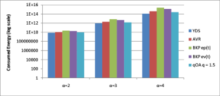
Figure 7: Energy consumption for a flat workload.

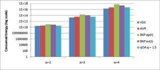
Figure 8: Energy consumption for a fixed span workload.

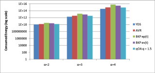
Figure 9: Energy consumption for a moderately spiky workload.

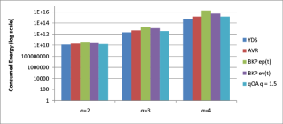
Figure 10: Energy consumption for a highly spiky workload.

What causes the relatively poor performance of ${\rm BKP}$? For our inputs, it seems to consistently choose a high speed at which to run. ${\rm BKP}$ needs to use a high multiplicative factor $e$ times its current estimated load in order to guarantee a feasible schedule. In addition, ${\rm BKP}$’s calculated speed can be increased by jobs that have already finished. Observe the ${\rm BKP}$ schedules depicted in Figures 11–14. The area under the curve appears partially filled because the algorithm keeps switching between a high speed and being idle (i.e. running at speed 0) because it has finished all released jobs. Comparison with Figures 1–4, which show the optimal schedule for the same workloads, confirms that ${\rm BKP}$ does indeed use much higher speeds than necessary.

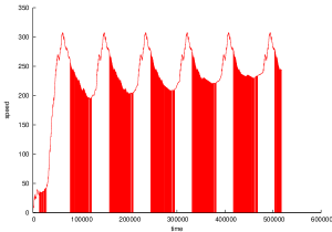
Figure 11: Plot of ${\rm BKP}$ $ev(t)$ schedule for a flat workload.

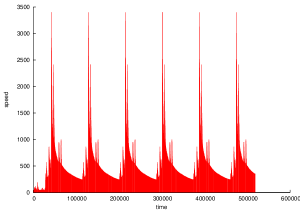
Figure 12: Plot of ${\rm BKP}$ $ev(t)$ schedule for a fixed span workload.

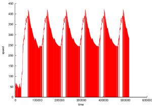
Figure 13: Plot of ${\rm BKP}$ $ev(t)$ schedule for a moderately spiky workload.

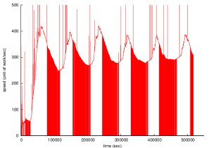
Figure 14: Plot of ${\rm BKP}$ $ev(t)$ schedule for a highly spiky workload.

Comparing the energy consumption of ${\rm BKP}$ schedules when speed is computed using $ep(t)$ and $ev(t)$, we notice that less energy is consumed when speed is computed using $ev(t)$. This is demonstrated in Figures 7–10. To see why this occurs, compare Figures 11 and 15, which respectively give the ${\rm BKP}$ schedules using $ev(t)$ and $ep(t)$ for the flat workload. Notice that the schedule using $ep(t)$ has higher peaks. This is not surprising given that it seems that both versions of ${\rm BKP}$ are running too fast at critical times, and we know that $v(t)\leq p(t)$.

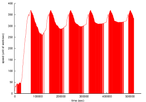
Figure 15: Plot of ${\rm BKP}$ $ep(t)$ schedule for a flat workload.

Our next several observations concern the optimal value of $q$ for algorithm ${\rm qOA}$ on different workloads. As noted above, the performance of ${\rm qOA}$ is not highly sensitive to the exact value of $q$, but its value nonetheless does matter. Our explanation for why different workloads favor different values of $q$ focuses on the spikes in schedule speed. These spikes have disproportionate affect on the energy consumption because raising speed to $\alpha$ causes the power to be much higher at these times due to the convexity of the power function. The spikes occur because the workload itself contains periods when more work arrives, but their height is affected by two factors related to the value of $q$. The first factor relates to the amount of work arriving before the spike that must be finished during it. A higher value of $q$ tends to reduce the amount of this type of work because higher $q$ causes ${\rm qOA}$ to run faster before the spike, thereby reducing the optimal speed during the spike. The second factor, which works against the first, is that ${\rm qOA}$ runs at $q$ times the optimal speed, including during the spike. Thus, a large value of $q$ may increase the speed of a spike even if the optimal speed during that time has been reduced. We believe that the optimal value of $q$ for different types of workloads is largely explained by the interaction of these factors on each type of workload.

First consider flat and moderately spiky workloads. For these workloads, the optimal value of $q$ is usually high— typically around 4 or higher. It is generally higher for moderately spiky workloads than for flat ones, as demonstrated in Figures 7 and 9. To explain these observations, we refer back to the optimal schedules for these workloads shown in Figures 1 and 3. These figures show that the spikes in the optimal schedule are fairly broad, with the optimal schedule for the flat workload exhibiting smaller spikes than the optimal schedule of the moderately spiky workload. The broad spikes allow the benefits of higher $q$ to be felt since finishing work early creates a narrower (but taller) spike. The difference between the workloads occurs because the flat workload, where the arrival rate of work varies less (smaller spikes in the optimal schedule), does not benefit as much from increasing $q$. The ${\rm qOA}$ schedules corresponding to the optimal schedules depicted in Figures 1 and 3 are shown in Figures 16 and 17.

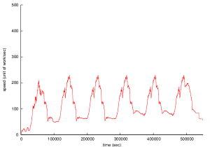
Figure 16: Plot of ${\rm qOA}$ schedule with $q=1.5$ for a flat workload.

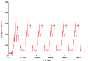
Figure 17: Plot of ${\rm qOA}$ schedule with $q=1.5$ for a moderately spiky workload.

As occurs in Figures 7 and 9, we observed that optimal $q$ usually increases with increasing $\alpha$ for both flat and moderately spiky workloads. Increasing $\alpha$ raises the penalty for having spikes in the schedule, so the workloads benefit from a slightly higher $q$, which finishes work slightly earlier and shrinks the spikes.

Now we turn our attention to the value of $q$ in fixed span and highly spiky workloads. For these workloads, optimal $q$ is usually very low (near 1), as demonstrated in Figures 8 and 10. To explain this, we again examine the optimal schedules for these workloads; see Figures 2 and 4. These optimal schedules have a number of very tall, very narrow spikes, indicating the arrival of a large amount of urgent work. The narrowness of the spike decreases the benefit of increasing $q$ because the schedule quickly runs out of urgent work. The height of the spike also increases the cost of large $q$ because running at a greater multiple of the optimal speed makes the tall spikes even taller. The ${\rm qOA}$ schedules corresponding to the optimal schedules depicted in Figures 2 and 4 are shown in Figures 18 and 19.

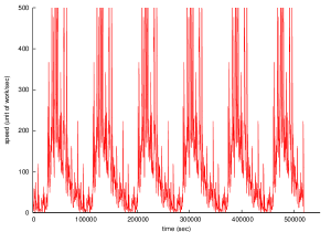
Figure 18: Plot of ${\rm qOA}$ schedule with $q=1.5$ for a fixed span workload.

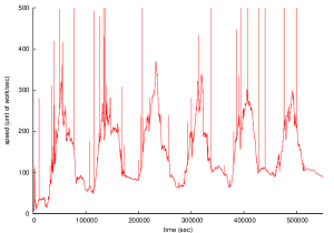
Figure 19: Plot of ${\rm qOA}$ schedule with $q=1.5$ for a highly spiky workload.

As $\alpha$ increases, the optimal value of $q$ for fixed span and highly spiky workloads decreased in our experiments (as demonstrated in Figures 8 and 10), which is consistent with the observation that increasing $\alpha$ increases the penalty for tall spikes.

Regarding the fixed span workload, the observation that optimal $q$ is near 1 holds for all the span lengths we tried. We offer a partial justification for this by discussing the extreme cases. With a short fixed span, there is little overlap between jobs and little reason to finish one before the next arrives since they are largely independent. With a long fixed span, there is a lot of overlap between the spans of jobs, allowing the optimal algorithm enough knowledge to find a good schedule, which then does not benefit by a speed increase. In both cases, the best $q$ will tend to be low.

In addition to comparing the algorithms with respect to energy consumption, we also compare them with respect to the maximum temperature reached by the schedules they compute. Our temperature calculations use a discrete approximation. We considered a range of values for the parameter $b$, and a time step of 0.1 seconds for the discrete approximation. We compared the algorithms using the parameters: $\alpha=2,3,4$, and a wide range of cooling parameters $b$. We found that the performance of the algorithms relative to each other with respect to temperature is the same as their relative performance with respect to energy consumption; from best to worst, the order was ${\rm YDS}$, ${\rm qOA}$, ${\rm AVR}$, ${\rm BKP}$ using $ev(t)$, and ${\rm BKP}$ using $ep(t)$. We did observe that the optimal value of $q$ for ${\rm qOA}$ could be slightly different for minimizing temperature than for minimizing energy consumption. (Although none of the algorithms take $\alpha$ into account when calculating speed, variations in $\alpha$ do favor differently shaped schedules.) Figure 20 plots maximum temperature as a function of the cooling parameter for the schedules produced by ${\rm BKP}$ $ev(t)$ and ${\rm qOA}$ ($q=1.5$) for a moderately spiky workload with $\alpha=3$.

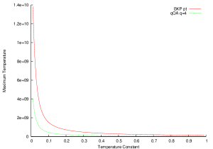
Figure 20: Plot of maximum temperature vs. cooling parameter for schedules of ${\rm BKP}$ $ev(t)$ and ${\rm qOA}$ with $q=1.5$, for a moderately spiky workload using $\alpha=3$

5 Conclusion

In summary, if you order the candidate speed scaling algorithms in the literature by the best competitive ratio that has been proved, this is exactly the order that these algorithms finished in our experimental horse race. We performed many more experiments than the representative sample that we report here, and we saw the same ordering of the algorithms across a wide range of different input distributions. So we don’t believe that these experimental results are due to any particularities in the input distributions that used. We thus believe that these experimental results can be viewed as a victory for competitive analysis as a predictor of experimental performance, even though that is the not the main goal of competitive analysis.

References

- [1] S. Albers, F. Müller, and S. Schmelzer. Speed scaling on parallel processors. In Proc. ACM Symposium on Parallel Algorithms and Architectures (SPAA), pages 289–298, 2007.
- [2] N. Bansal, D.P. Bunde, H.-L. Chan, and K. Pruhs. Average rate speed scaling. In Latin American Theoretical Informatics Symposium, 2008.
- [3] N. Bansal, H.-L. Chan, and K. Pruhs. Improved bounds for speed scaling in devices obeying the cube-root rule. In SODA, 2009. submitted.
- [4] N. Bansal, T. Kimbrel, and K. Pruhs. Speed scaling to manage energy and temperature. JACM, 54(1), 2007.
- [5] N. Bansal and K. Pruhs. Speed scaling to manage temperature. In STACS, pages 460–471, 2005.
- [6] H.-L. Chan, W.-T. Chan, T.-W. Lam, L.-K. Lee, K.-S. Mak, and P.W. H. Wong. Energy efficient online deadline scheduling. In SODA ’07: Proceedings of the eighteenth annual ACM-SIAM symposium on Discrete algorithms, pages 795–804, 2007.
- [7] W.-C. Kwon and T. Kim. Optimal voltage allocation techniques for dynamically variable voltage processors. In Proc. ACM-IEEE Design Automation Conf., pages 125–130, 2003.
- [8] M. Li, B.J. Liu, and F.F. Yao. Min-energy voltage allocation for tree-structured tasks. Journal of Combinatorial Optimization, 11(3):305–319, 2006.
- [9] M. Li and F.F. Yao. An efficient algorithm for computing optimal discrete voltage schedules. SIAM J. on Computing, 35:658–671, 2005.
- [10] F. Yao, A. Demers, and S. Shenker. A scheduling model for reduced CPU energy. In Proc. IEEE Symp. Foundations of Computer Science, pages 374–382, 1995.