Analysis of slope-intercept plots for arrays of electron field emitters

Abstract

In electron field emission experiments, a linear relationship in plots of slope vs. intercept obtained from Fowler-Nordheim analysis is commonly observed for single tips or tip arrays. By simulating samples with many tips, it is shown here that the observed linear relationship results from the distribution of input parameters, assuming a log-normal distribution for the radius of each tip. Typically, a shift from the lower-left to the upper-right of a slope-intercept plot has been correlated with a shift in work function. However, as shown in this paper, the same effect can result from a variation in the number of emitters.

I Introduction

Field emitters such as carbon nanofibers play an important role in today’s vacuum electronics.Gaertner (2012) They are also used in ion sources, for example field ionization sources for neutron generators. Naranjo, Gimzewski, and Putterman (2005); Resnick et al. (2010); Ellsworth et al. (2013); Persaud et al. (2012, 2011) In all cases, it is important to be able to characterize the field emitter samples, which can be done using electron field emission experiments, see for example Ref. Waldmann et al., 2013.

Electron field emission occurs as a result of a tunneling process of electrons through a potential barrier. This was first reported by Fowler and Nordheim in 1928,Fowler and Nordheim (1928) who derived an equation for the emitted current. In their 1-dimensional model, the emission current is expressed as a function of the local field, the emitter area, and the work function of the material. Since then, the model has been extended to include a number of correction factors.Forbes, Fischer, and Mousa (2013)

The Fowler-Nordheim (FN) equation can be rewritten using a different set of variables, such that the relationship between these new variables is linear. The linear fit results in two parameters: the slope and the intercept. If one acquires several FN-plots for the same sample or for a set of different samples, different slope-intercept data points are obtained. When plotting the slope against the intercept, an almost linear relationship has been observed in many cases. Mackie et al. (2003); Charbonnier, Southall, and Mackie (2004); Gotoh et al. (2007a); Kawasaki et al. (2010) It has not been clear what the origin of this linear relationship is or what it implies. In this paper, the linearity is explained using a statistical model simulating field emission from tips with a random distribution of height, radius, and work function.

II Theory

In the following, the equations used for the simulations presented in this paper are introduced. For an introduction into the theory of field emission, the reader is referred to Gomer, Gomer (1994) and for a short summary to the article on FN-analysis by Forbes et al.Forbes (2012); Forbes, Fischer, and Mousa (2013)

The simplest equation for FN-tunneling is given by

$$I=\frac{c_{a}AE_{local}^{2}}{\Phi}\exp\left(\frac{-c_{b}\Phi^{1.5}}{E_{local}}\right),$$ (1)

where $I$ is the emitted current, $c_{a}$ and $c_{b}$ are the so-called first and second FN-constants, $A$ is the emitting area, $\Phi$ is the work function of the material, and $E_{local}$ is the local electric field. The values for the FN-constants are $c_{a}=\frac{e^{3}}{16\pi^{2}\hbar}=1.5414\times 10^{-6}\,\nicefrac{\mathrm{AeV}}{\mathrm{V^{2}}}$ and $c_{b}=\frac{4\sqrt{2m_{e}}}{3e\hbar}=6.8309\times 10^{9}\,\nicefrac{\mathrm{Vm}}{\mathrm{eV^{1.5}}}$, with $e$, $m_{e}$, being the charge and mass of an electron, respectively, and $\hbar$ being the reduced Planck constant.

The local field can be expressed using the applied field $E$ and a local field enhancement factor $\gamma$, as

$$E_{local}=\gamma E.$$ (2)

Equation (1) is derived for the 1-dimensional case and a uniform applied field. In experiments, the field is enhanced at a step or a sharp point. The enhancement factor $\gamma$ directly expresses the amount of enhancement from a tip-like structure compared to a flat surface. For cylindrical tips, a simple estimate is given by

$$\gamma_{simple}=\frac{H}{R},$$ (3)

where $H$ is the height of the tip and $R$ the radius. A more precise estimate is given by Edgcombe and Valdrè Edgcombe and Valdre (2001) as

$$\gamma=1.2\left[\frac{H}{R}+2.5\right]^{0.9}.$$ (4)

If there are many emitters in an array structure, there is also a shielding effect that needs to be taken into account, especially if the tips are very close to each other. The shielding effect can be estimated Bonard et al. (2001); Jo et al. (2003) using

$$\gamma_{array}=\gamma\left[1-\exp\left(-2.3171\frac{S}{H}\right)\right],$$ (5)

where $S$ is the spacing between the tips.

It can be helpful to rescale the FN-equation using

$$f=\frac{c_{S}^{2}}{\Phi^{2}}E_{local},$$ (6)

where $c_{S}$ is the Schottky constant ($c_{S}^{2}=\frac{e^{3}}{4\pi\epsilon_{0}}$; $\epsilon_{0}$ is the electric constant). By doing this, the FN-equation now depends on a dimensionless variable. Using this rescaling approach and adding some correction factors, the FN-equation can be written as Forbes, Fischer, and Mousa (2013)

$$I=Ac_{a}\frac{\Phi^{3}}{c_{S}^{4}}f^{2}\exp\left(-\frac{c_{b}c_{S}^{2}}{\sqrt{\Phi}}\left[1-f+\frac{1}{6}f\ln(f)\right]\frac{1}{f}\right).$$ (7)

This equation is physically more realistic than Eq. (1), since it takes image forces into account. This has the effect that the tunneling barrier is lower compared to the case in Eq. (1), and higher emission currents (typically by a factor of 100 or more) are predicted.

The linear relationship of the FN-plot is seen when rewriting Eq. (1) as

$$\ln\left(\frac{I}{E^{2}}\right)=\ln\left(\frac{c_{a}A\gamma^{2}}{\Phi}\right)-\frac{c_{b}\Phi^{1.5}}{\gamma}\frac{1}{E}.$$ (8)

Clearly, this equation has the linear form,

$$\ln\left(\frac{I}{E^{2}}\right)=b+m\frac{1}{E}.$$ (9)

More realistic equations, such as equation (7), generate nearly (but not exactly) linear FN-plots. These more realistic theoretical plots, and also many experimental FN-plots, can in practice be fitted by a linear equation of form Eq. (9). In all the figures in this paper, the quantity $\frac{I}{E^{2}}$ is expressed in the units ($\mathrm{AV^{-2}m^{2}}$) before the natural logarithm is taken.

From the slope $m$ and the intercept $b$ of the fit, one can calculate two of the three parameters $A$, $\Phi$, and $\gamma$, if one makes an assumption about the third parameter. Often one assumes a known value for the work function in order to extract the other two parameters. Due to the form of the equation, it is not easy to obtain information on the work function and the field enhancement factor at the same time, since they appear almost as $\frac{\Phi}{\gamma}$, which makes them difficult to distinguish. Furthermore, it is non-trivial to define the emitting area. This is due to the fact that the original equation was derived for the 1-dimensional case, whereas for a 3-dimensional sharp tip the electric field will not be constant across the surface and there will be a field dependence of the area that is not included in these equations. In addition, time dependence of any of the parameters is not included in this analysis. Time dependent effects include changes in the work function and field enhancement factors due to absorbents on the surface or blunting of the tips due to sputtering or heating effects.

III Slope-intercept plots

In order to compare different samples or to examine the behavior of a single sample over time, plotting the slope and intercepts from fitting different FN-plots was introduced.Ishikawa et al. (1993); Gotoh et al. (1996) Often these plots are also referred to using their Japanese names: Seppen-Katamuki plots or SK-plots for short. From Eq. (1), one can calculate lines of constant work function or constant field enhancement factor for these plots. Assuming one of the relationships between radius, height, and field enhancement factors listed above, equations for constant height and constant radius can also be derived.Ishikawa et al. (1993); Gotoh et al. (1996); Mackie et al. (2003); da Rocha et al. (2008); Kawasaki et al. (2010); Nicolaescu et al. (2001)

In SK-plots, a linear relationship between the slope and the intercept is often observed. Gotoh et al. (2007b); Ishikawa et al. (1993); Gotoh et al. (1996); Kawasaki et al. (2010) However, this linear relationship cannot easily be explained assuming only a change in a single parameter, such as the radius. For a possible explanation using the simple FN-equation, one needs to assume a more complex radial dependency of the area.Ishikawa et al. (1993); Gotoh, Tsuji, and Ishikawa (2001) Another problem with explanations of this kind can be seen if one looks at data from repeated experiments, for example, as shown in Figure 7 in the paper of Gotoh et al.Gotoh et al. (2004) The data points do not start at one end of the line and then move along to the other end, as one would expect if the change would be due to a continuous function, but rather the distribution of data points along the line appears to be random.

The linear relation shown in the SK-plots seems to be orthogonal to a change in work function and therefore different parallel lines in a SK-plot have been attributed to a change in the work function and absolute values have been extracted. A good example of this can be seen in the work of Gotoh et al.,Gotoh et al. (2007b) where the authors were able to extract the work functions for different crystal planes of a tungsten emitter.

Charbonnier, Southall, and Mackie also investigated further possible explanations for the linear behavior in SK-plots, and considered whether nano-protrusions on top of a single emitter can be the cause. They found that a single protrusion cannot fit the experimental data, but if several protrusions are used then good linear fits to the SK-plots can be obtained by choosing the correct parameters for these protrusions. Charbonnier, Southall, and Mackie (2004)

IV Simplified model

For an array of $N$ tips, the FN-equation becomes more complicated, since one has to deal with many tips that will show a distribution of heights, radii and work functions. Also, the shielding between tips cannot be easily computed, since neighboring tips will have different heights and radii and therefore the shielding effect will vary. The shielding effect can be neglected, however, if the distance between tips is larger than twice the height of the tips.Bonard et al. (2001) From here on, the assumption is made that the tips on the sample are spaced even further apart and therefore any shielding effect is ignored. To make the model very simple, Eqs. (1)– (3) are used. The index $i$ is used to distinguish different tips, that is, $R_{i}$ will be the radius of tip $i$, etc. Furthermore, a very basic relation for the area of each tip, $A_{i}=\pi r_{i}^{2}$, is assumed. The total current for a single sample can then be written as

$$I=\sum_{i}^{N}\frac{c_{a}\pi H_{i}^{2}E^{2}}{\Phi_{i}}\exp\left(\frac{-c_{b}\Phi_{i}^{1.5}R_{i}}{H_{i}E}\right).$$ (10)

Nicolaescu et al. have used a similar equation to directly fit FN-plots using parameters of the distribution as fitting parameters. Nicolaescu et al. (2003, 2004)

The distribution of most parameters is most likely a log-normal distribution (negative values for height and radius from a normal Gaussian distribution would not make sense). A log-normal distribution for the radius has also been observed by Ding et al.,Ding, Sha, and Akinwande (2002); Nicolaescu et al. (2006) as well as by Park et al. for the field enhancement factor.Park, Lee, and Koh (2006)

V Simulation results

In the following, the results of simulations using Eq. (10) with varying parameters are shown. The difference between a simple model and using the more realistic FN-equation (7), and the different approximations for the field enhancement factors are also examined. Various random distributions are explored (log-normal, normal, uniform), as well as the effect of just using a constant value. When comparing a log-normal/Gaussian distribution with a uniform distribution, the range in values for the uniform distribution is chosen to coincide with six standard deviations of the log-normal/Gaussian distribution. Histograms of example distributions are plotted in Fig. 1.

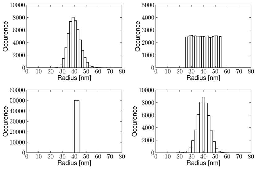
Figure 1: The investigated distributions using the radial distribution as an example. Top row: log-normal distribution, uniform distribution, bottom row: constant value, Gaussian distribution.

The simulations were carried out using python.Foundation (95) The numerical python module numpyJones et al. (01) was used for most of the calculations and for random number generation, pylabHunter (2007) was used for plotting, scipyJones et al. (01) was used for the fitting routine, and ipythonPérez and Granger (2007) was utilized to execute the main routine in parallel on a local ipcluster. The basic algorithm consisted of the following steps for calculating $K$ samples of size $S$: a) generate $S$ random distributed values for radius, height and work function, and calculate field enhancement factors for each tip; b) for a given range of applied electric field, calculate the total current for the sample for each field value; c) perform a linear fit on the simulated data using Eq. (9) and save the fit parameters; d) repeat steps a)-c) $K$ times to generate statistics; e) plot results.

For the following results, the values shown in Table 1 are used unless otherwise noted. The electric fields used for the fit were 20 evenly spaced values between $1.6\,\nicefrac{\mathrm{V}}{\mathrm{\mu m}}$ and $26\,\nicefrac{\mathrm{V}}{\mathrm{\mu m}}$.

Parameter	Radius	Height	Work function
Average $\mu$	40 nm	6 $\mu$m	4.8 eV
Deviation $\sigma$	5 nm	0.1 $\mu$m	0.3 eV

Table 1: Parameters used in the simulation. For a uniform distribution, the minimum and maximum values are taken as $\mu\pm 3\sigma$ and for constant values just the value for $\mu$ is used.

In Figs. 2 and 3, results are plotted for a sample with a constant height and a constant work function, but different radial distributions: uniform and log-normal. Furthermore, the number of tips per sample, $N$ in Eq. (10), is varied as shown in the plots. One can see that a nearly linear relationship emerges for large $N$ and a log-normal distribution of tip radii.

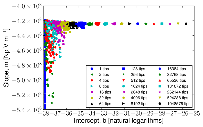
Figure 2: SK-plot for uniform radial distribution, constant height and work function, variation in sample size. For each sample size 100 samples have been simulated.

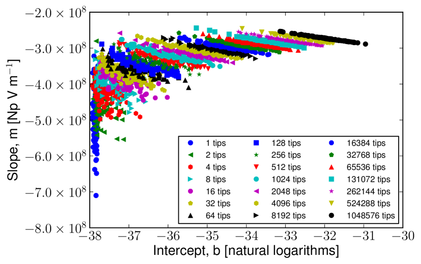
Figure 3: SK-plot for log-normal radial distribution, constant height and work function, variation in sample size. For each sample size, 100 samples have been simulated.

This emerging behavior is purely statistical in nature due to the fact that a log-normal distribution has a non-zero probability of containing very sharp tips. However, when one looks more closely at a single SK-plot and generates better statistics, a different picture is revealed. A histogram of a simulation using 128 emitters per sample for a total of 5000 samples is shown in Fig. 4

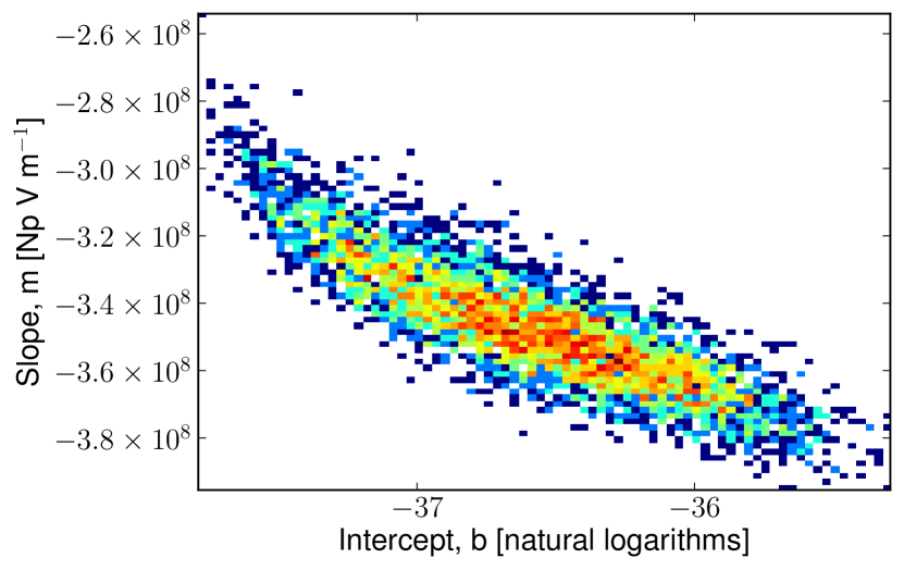
Figure 4: SK-plot for log-normal radial distribution, log-normal height, and constant work function, sample size 128. 5000 samples have been simulated.

and shows that instead of a linear relationship the SK-plot is actually closer to a 2-dimensional Gaussian distribution, which would be expected for large numbers. From Fig. 3, it is clear that the greater the number of tips/sample the narrower the 2-dimensional Gaussian distribution will be, resulting in the almost linear appearance.

In Fig 5, the dependency of the

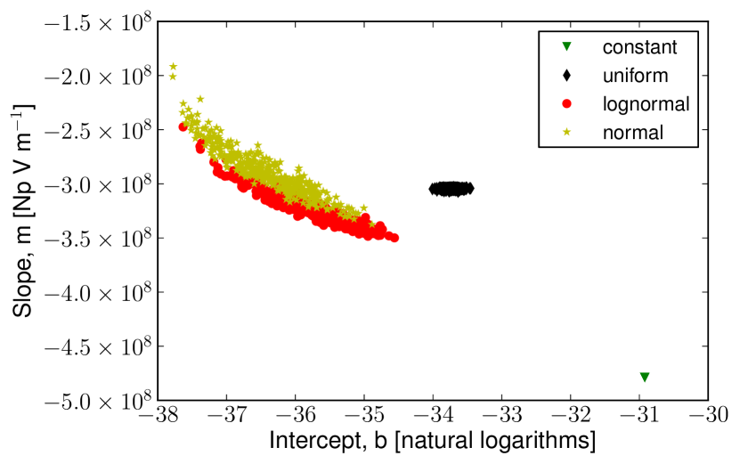
Figure 5: SK-plot for constant height and work function with varying distributions for the radius. Sample size 1024 tips, 400 samples have been simulated for each distribution.

shape of the SK-plot on the type of radial distribution is explored. Obviously, if only constant values are used, all data points in the SK-plot are the same. A uniform distribution for the radius results in a horizontal distribution of points that only varies slightly on the SK-plot. This is similar to plots of constant radius in previous publications, although using a simpler model for the dependency of the FN-equation on tip radius. A log-normal or Gaussian distribution, however, shows an almost linear spread across a wide range of values in the SK-plot, very similar to experimental observations.

It is also easy to simulate the effect of the different approximations for the field enhancement factor (Eqs. (3)–(5)). The results are shown in Fig. 6. Although there is a shift in values, the shape of the resulting plot does not change. Therefore, for the purpose of this paper the use of the simplest approximation is justified.

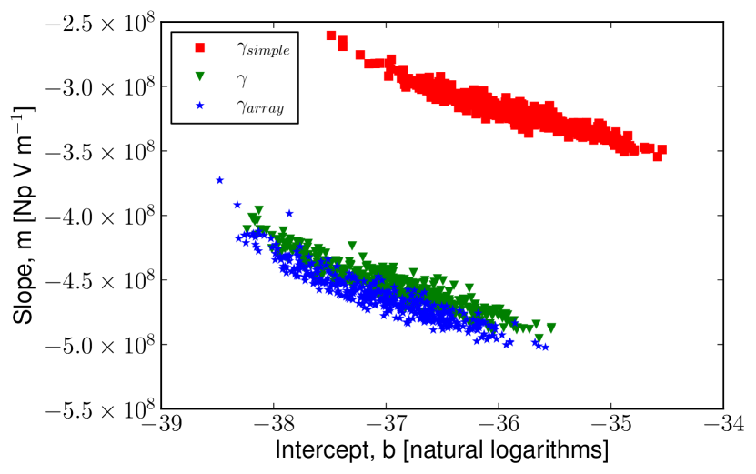
Figure 6: SK-plot for log-normal radial distribution, log-normal height, and constant work function. Comparing the effect of different approximations on the field enhancement factor. For the array simulation a spacing of $10\,\mathrm{\mu m}$ was assumed.

Similarly, the simple FN-equation yields the same results compared to the more realistic one, as seen in Fig. 7.

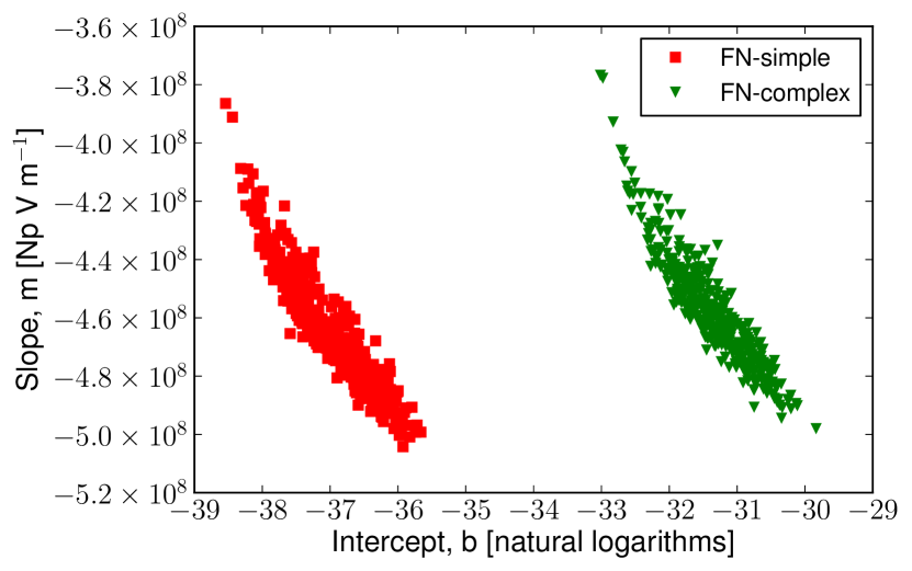
Figure 7: SK-plot for log-normal radial distribution, log-normal height, and constant work function. Comparing the use of the simple FN-equation vs. the more complex one. Each simulation used 400 samples with 1024 tips.

In addition, using different distributions for the height does not influence the shape of the SK-plots, as can be seen in Fig. 8.

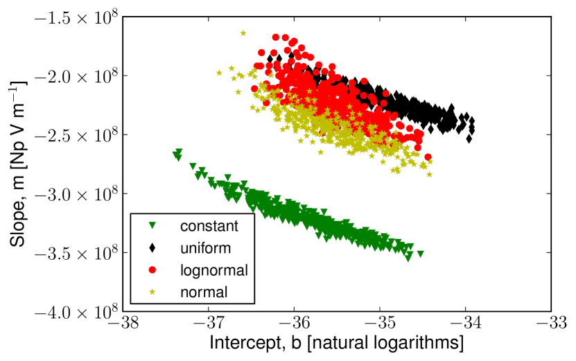
Figure 8: SK-plot for log-normal radial distribution and constant work function. Varying the type of distribution for the height. Each simulation used 400 samples with 1024 tips.

In Fig. 9, different SK-plots

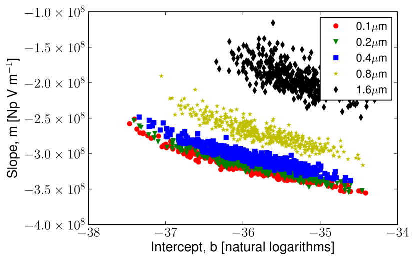
Figure 9: SK-plot for log-normal radial distribution, log-normal height, and constant work function. Varying the standard deviation of the height distribution. Each simulation used 400 samples with 1024 tips.

are shown for a log-normal height distributions with different standard deviations. The width of the resulting plot and the position vary, but the distributions along the length of the SK-plot seem to be dominated by the radial distribution for this parameter space.

Finally, the distribution of different work function values with SK-plots for different sample sizes are compared. In Fig. 10, one can see that it is impossible to distinguish a work function change of 0.3 eV and a change in sample size of a factor of $4$.

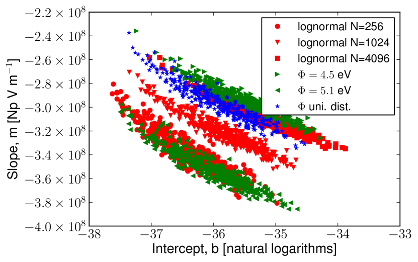
Figure 10: Comparing different sample sizes with a change in work function. All simulations use a constant value for the height and the work function, unless otherwise noted. The simulation used 400 samples for each case and 1024 tips, unless otherwise noted.

A distribution of work function values also only slightly influences the shape of the SK-plot. The resulting SK-plot for a work function that is not constant across a sample is wider than that for a constant work function sample, and tends to be similar in values to a higher work function sample.

VI Conclusions

As shown, experimental electron field-emission data obtained using tip arrays can be reproduced assuming a simple model and a log-normal distribution of tip radii. The model can explain the spread observed in the SK-plots and the almost linear relationship observed, as well as the fact that the data points appear randomly along the line of the plot. The effect seems to be purely statistical in nature due to the finite number of tips on each sample and the fact that a log-normal distribution produces a few very sharp tips leading to a larger distribution in the emitted current. Since the calculations were carried out for arrays of tips, it is not immediately clear how the almost linear form of an SK-plot can also be reproduced for single tips.Kawasaki et al. (2010) One can speculate that this is due to statistical variations in nano-protrusions on the tip surface, which for a small number of protrusions has been shown to result in a similar effect.Charbonnier, Southall, and Mackie (2004) Similarly, for repeated measurements on a single sample, the observation of nearly linear SK-plots indicates that the radial distributions change over time while still following a log-normal or similar distribution.

The simulations also show that a change in work function will shift the SK-plot, supporting analyses conducted elsewhere, as for example in the paper of Gotoh et al.Gotoh et al. (2007b) However, the simulations also show that changes in the number of emitters per sample give similar results to those obtained when varying the work function. Therefore, if the number of emitters is not well known, no conclusion about the work function can be made.

It will not be possible to extract all distribution parameters from measured data using this model, since changes in several parameters lead to the same effect, for example, changes in work function vs. changes in sample size, or changes in standard deviation of the height distribution vs. a distribution of work function values. This is similar to the known fact that one cannot extract the field enhancement factor and the work function reliably at the same time from a single FN-plot. However, when assumptions can be made for several of the parameters one should be able to extract information from the sample by creating SK-plots with good statistics. Here, one has to make sure that the correction factors are used, since these can create large offsets in the absolute values of slope and intercept, as shown. The extraction of distribution parameters using this approach will be explored in a future publication.

References

- Gaertner (2012) G. Gaertner, J. Vac. Sci. Technol. B 30, 060801 (2012).
- Naranjo, Gimzewski, and Putterman (2005) B. Naranjo, J. K. Gimzewski, and S. Putterman, Nature 434, 1115 (2005).
- Resnick et al. (2010) P. Resnick, C. Holland, P. Schwoebel, K. Hertz, and D. Chichester, Microelectronic Engineering 87, 1263 (2010).
- Ellsworth et al. (2013) J. L. Ellsworth, V. Tang, S. Falabella, B. Naranjo, and S. Putterman, AIP Conf. Proc. 1525, 128 (2013).
- Persaud et al. (2012) A. Persaud, O. Waldmann, R. Kapadia, K. Takei, A. Javey, and T. Schenkel, Rev. Sci. Instrum. 83, 02B312 (2012).
- Persaud et al. (2011) A. Persaud, I. Allen, M. R. Dickinson, T. Schenkel, R. Kapadia, K. Takei, and A. Javey, J. Vac. Sci. Technol. B 29, 02B107 (2011).
- Waldmann et al. (2013) O. Waldmann, A. Persaud, R. Kapadia, K. Takei, F. I. Allen, A. Javey, and T. Schenkel, Thin Solid Films 534, 488 (2013).
- Fowler and Nordheim (1928) R. H. Fowler and L. Nordheim, Proc. R. Soc. London. Ser. A 119, 173 (1928).
- Forbes, Fischer, and Mousa (2013) R. G. Forbes, A. Fischer, and M. S. Mousa, J. Vac. Sci. Technol. B 31, 02B103 (2013).
- Mackie et al. (2003) W. A. Mackie, L. A. Southall, T. Xie, G. L. Cabe, F. M. Charbonnier, and P. H. McClelland, J. Vac. Sci. Technol. B 21, 1574 (2003).