The 2d XY model exhibits an essential phase transition, which was predicted long ago — by Berezinskii, Kosterlitz and Thouless (BKT) — to be driven by the (un)binding of vortex–anti-vortex pairs. This transition has been confirmed for the standard lattice action, and for actions with distinct couplings, in agreement with universality. Here we study a highly unconventional formulation of this model, which belongs to the class of topological lattice actions: it does not have any couplings at all, but just a constraint for the relative angles between nearest neighbour spins. By means of dynamical boundary conditions we measure the helicity modulus $\Upsilon$, which shows that this formulation performs a BKT phase transition as well. Its finite size effects are amazingly mild, in contrast to other lattice actions. This provides one of the most precise numerical confirmations ever of a BKT transition in this model. On the other hand, up to the lattice sizes that we explored, there are deviations from the spin wave approximation, for instance for the Binder cumulant $U_{4}$ and for the leading finite size correction to $\Upsilon$. Finally we observe that the (un)binding mechanism follows the usual pattern, although free vortices do not require any energy in this formulation. Due to that observation, one should reconsider an aspect of the established picture, which estimates the critical temperature based on this energy requirement.

E-mail:  wolbi@nucleares.unam.mx,  gerber@correo.nucleares.unam.mx,
               f.rejon@student.uva.nl

1 The 2d XY model and its constraint lattice action

The 2d XY model is one of the simplest models in quantum field theory and statistical mechanics. It has been studied extensively since the 1970s, but interesting aspects are still being revealed.

This model describes certain systems in solid state physics, in particular superfluid helium films [1], which is reflected by the global $O(2)$ symmetry. Further applications include superconducting films [2], the Coulomb gas model [3], Josephson junction arrays [4] and nematic liquid crystals [5]. The applications are not as broad as for the (even simpler) Ising model, but the phase transition in the XY model is conceptually more interesting. It is one of the few examples in the literature for a transition beyond second order; more precisely it is of infinite order, and therefore an essential phase transition, known as the Berezinskii-Kosterlitz-Thouless (BKT) transition [6, 1]. BKT phase transitions have been identified also in other models, which could be solved exactly [7].

In the 2d XY model, the key to its understanding are the vortices and anti-vortices [6, 1]. Entire configurations do not have distinct topological charges, but in a square lattice regularisation each plaquette carries a winding number $0$, $+1$ (vortex) or $-1$ (anti-vortex). The dynamics of these topological defects turned out to be crucial for the phase diagram.

Here we stay within the framework of formulations on an $L\times L$ square lattice, with a classical spin $\vec{e}_{x}$ attached to each site $x$,

$$\vec{e}_{x}=\left(\begin{array}[]{c}\cos\phi_{x}\\ \sin\phi_{x}\end{array}\right)\in{\kern 2.5pt\sf{R}\kern-7.79999pt\sf{I}\kern 7.79999pt\kern-2.5pt}^{2}\ ,$$ (1.1)

such that $|\vec{e}_{x}|=1\,,\ \forall x\,$. The standard action on the lattice (in lattice units) reads

$$S[\vec{e}\,] = \sum_{\langle xy\rangle}s(\vec{e}_{x},\vec{e}_{y})\ ,$$

$$s(\vec{e}_{x},\vec{e}_{y}) = \beta\Big{(}1-\vec{e}_{x}\cdot\vec{e}_{y}\Big{)}=\beta\Big{(}1-\cos(\phi_{x}-\phi_{y})\Big{)}\ ,$$ (1.2)

where the sum runs over all nearest neighbour sites $x$, $y$, and $\beta>0$ is the inverse coupling. Its critical value for the BKT transition was identified as $\beta_{\rm c}=1.1199(1)$ [8] (earlier determinations of $\beta_{\rm c}$ are quoted in Refs. [9, 10]).

The mechanism behind the BKT phase transition was understood based on the density of free vortices (and anti-vortices):

• At $\beta>\beta_{\rm c}$ this density is low, so that a kind of long-range order emerges. The correlations only decay with a power law, so the correlation length $\xi$ is infinite (massless phase). Most of the topological defects occur as tightly bound vortex–anti-vortex pairs, which appear topologically neutral from a large-scale perspective, hence these objects do not prevent the long-range order.

• As $\beta$ decreases below $\beta_{\rm c}$, a significant number of these pairs dissociate, so the density of free vortices jumps up. This destroys the long-range order, and $\xi$ becomes finite (massive phase). The value of $\beta_{\rm c}$ has been estimated from the energy that a free vortex requires [1].

This picture was originally in competition with other proposed scenarios, but it is now generally accepted since it led to correct quantitative predictions. They include the exponential divergence of $\xi$ at $\beta\mathop{\raise 1.29167pt\hbox{$<$\kern-7.5pt\raise-4.73611pt\hbox{$\sim$}}}\beta_{\rm c}$ as [11]

$$\xi\propto\exp\Big{(}\frac{\rm const.}{(\beta_{\rm c}-\beta)^{\nu}}\Big{)}\ ,\qquad\nu_{\rm c}=1/2\ ,$$ (1.3)

which characterises the essential phase transition. If we approach the BKT transition from the other side, i.e. within the massless phase, on large $L\times L$ lattices, this picture predicts the magnetic susceptibility $\chi$ to diverge as [11]

$$\chi\propto L^{2-\eta}\ (\ln L)^{-2r}\ ,\quad\eta_{\rm c}=1/4\ ,\quad r_{\rm c}=-1/16\ .$$ (1.4)

The numerical verification of the critical exponents $\eta_{\rm c}$ and $r_{\rm c}$ has been a long-standing challenge, despite the simplicity of the model, due to the tedious logarithmic finite size effects (see Ref. [10] for an overview). The most satisfactory confirmation of these values was reported in Ref. [12], based on simulations of the action (1.2) on lattices up to size $L=2048$.

The mapping of this system onto the sine-Gordon model also provides analytic predictions for the Step Scaling Function [13]. Again numerical simulations of the standard action yield a plausible confirmation, if one refers to a specific ansatz for the finite size scaling [14].

Lattice actions with additional spin couplings, such as the Villain action [3], lead to the same continuum extrapolation, as expected due to the general principle of universality. However, this property is less clear for the highly unconventional topological lattice actions [15], which are invariant under (most) small deformations of a spin configuration. The formulation of the 2d XY model by topological lattice actions was recently discussed in Ref. [16]. Here we address the most radical variant, the constraint action, which does not have any spin couplings at all. Instead the relative angles between nearest neighbour spins are constrained to some maximum $\delta$. Hence the contribution of such a spin pair to the action amounts to

$$s(\vec{e}_{x},\vec{e}_{y})=\left\{\begin{array}[]{cccc}0&&&\vec{e}_{x}\cdot\vec{e}_{y}>\cos\delta\\ +\infty&&&{\rm otherwise}\end{array}\right.\ .$$ (1.5)

Therefore all configurations which violate this constraint for at least one spin pair $(\vec{e}_{x}$, $\vec{e}_{y})$ are excluded from the functional integral, while all other configurations have the same action $S[\vec{e}\,]=\sum_{\langle x,y\rangle}s(\vec{e}_{x},\vec{e}_{y})=0$. Obviously the concept of a classical limit — which corresponds to the action minimum — does not apply here, and perturbation theory neither. Instead there is an enormous degeneracy, since all allowed configurations have the same action.

For increasing $\delta$ a transition from a massless to a massive phase was observed [16]. In particular, at $\delta\mathop{\raise 1.29167pt\hbox{$>$\kern-7.5pt\raise-4.73611pt\hbox{$\sim$}}}\delta_{\rm c}$ the correlation length could be fitted well to the behaviour analogous to relation (1.3),

$$\xi\propto\exp\Big{(}\frac{\rm const.}{\sqrt{\delta-\delta_{\rm c}}}\Big{)}\ .$$ (1.6)

This observation is based on measurements of $\xi$ on $L\times L$ lattices with $L=500$, $1000$ and $2000$. In the range $\delta=1.89\dots 2$, $\xi$ increases from $17.65(5)$ to $251.2(2)$. Referring to values which are converged (for fixed $\delta$ and increasing $L$), we evaluated $\delta_{\rm c}$ by a fit to the ansatz (1.6), which yields

$$\delta_{\rm c}=1.775(1)\ .$$ (1.7)

As another aspect, the evaluation of the critical exponent $\nu_{\rm c}$ will be discussed in Subsection 3.1.

Also the fits of the susceptibility $\chi$ to the form (1.4) attained a good quality for large volumes, $L=128\dots 4096$. Hence we did observe a behaviour, which is compatible with a BKT transition at $\delta_{\rm c}$, though this type of transition could not be singled out unambiguously. The precision of that study was again limited by the logarithmic finite size effects.

Here we are going to revisit this phase transition for the constraint action. Section 2 deals with the helicity modulus. Its numerical measurement is not straightforward for topological lattice actions. It is achieved nevertheless by the use of dynamical boundary conditions. Section 3 addresses the second moment correlation length $\xi_{2}$ and the Binder cumulant $U_{4}$. We give results for the constraint action and for the standard action, which are compared to predictions of the spin wave approximation. Section 4 discusses the statistics and correlations of vortices and anti-vortices, and the density of “free vortices”. We study their dependence on the constraint angle $\delta$, and verify the pair (un)binding mechanism for the BKT transition in this unconventional formulation, where free vortices can appear without any energy cost (at $\delta>\pi/2$). Three appendices are devoted to the algorithmic tools that we employed, and to the difficulty in formulating a cluster algorithm for simulations with dynamical boundary conditions.

2 The helicity modulus

The helicity modulus $\Upsilon$ is a quantity that condensed matter physics often refers to. It is sometimes also denoted as “spin stiffness” or “spin rigidity”, and it is proportional to the “superfluid density”. It appears in the literature on $O(4)$ models [18] in a form, which would be called a Low Energy Constant in the terminology of Chiral Perturbation Theory. In that context, it is related to the pion decay constant $F_{\pi}$ as $\Upsilon\propto F_{\pi}^{2}$ [19].

$\Upsilon$ is a measure for the sensitivity of a system to torsion, i.e. to a variation of a twist in the boundary conditions [18]. This is often a useful indicator to characterise a universality class, in addition to the critical exponents and the Step Scaling Function.

2.1 Definition and prediction

For a conventional (non-topological) action on an $L\times L$ lattice, $\Upsilon$ can be defined as

$$\Upsilon=\frac{\partial^{2}}{\partial\alpha^{2}}F(\alpha)|_{\alpha=0}\ ,$$ (2.1)

where $F=-\frac{1}{\beta}\ln Z$ is the free energy, and $Z$ is the partition function. Here we assume the boundary conditions to be periodic in one direction, and twisted with the angle $\alpha$ in the other one. $F$ is minimal at $\alpha=0$, hence $\Upsilon$ corresponds to the curvature in this minimum.

Once we are dealing with topological lattice actions, these notions need to be modified. In particular for the constraint action (1.5) there is no coupling, hence we consider the dimensionless helicity modulus

$$\bar{\Upsilon}:=\beta\,\Upsilon\ .$$ (2.2)

For the 2d XY model in a square volume, the critical value at the BKT transition was first predicted analytically [20] as $\bar{\Upsilon}_{\rm c,\,theory}=\frac{2}{\pi}.$ Later a tiny correction (below $0.2$ per mille) due to winding configurations was identified in Ref. [21] (see also Ref. [12]), which leads to

$$\bar{\Upsilon}_{\rm c,\,theory}=\frac{2}{\pi}\Big{(}1-16\pi e^{-4\pi}\Big{)}\simeq 0.636508\ .$$ (2.3)

2.2 Methods of the numerical measurement

For the standard lattice action, there is a convenient way to measure $\bar{\Upsilon}$ at $\alpha=0$, such that the generation of configurations can be restricted to periodic boundary conditions [22]. The most extensive numerical study that evaluated $\bar{\Upsilon}$ in this way was performed by M. Hasenbusch [12]; his results are included in Figure 5. In his largest system, $L=2048$, he obtained at $\beta_{\rm c}=1.1199$ the value $\bar{\Upsilon}_{\rm c}=0.67246(10)$, which is still $5.6~{}\%$ too large. For the infinite volume extrapolation, he fitted his results for various sizes $L$ to the form

$$\bar{\Upsilon}_{\rm c}(L)=\bar{\Upsilon}_{\rm c,\,theory}+\frac{c_{1}}{\ln L+c_{2}}\ ,$$ (2.4)

with free parameters $c_{1},\ c_{2}$, which worked decently. Ref. [12] also derived the theoretical prediction

$$c_{1}\simeq 0.3189$$ (2.5)

in the spin wave limit, which was compatible with the fit to the data for the standard action. This prediction is based on the mapping onto the Gaussian model, where the parameter $\beta$ is inverted. Further arguments in favour of the universality of the coefficient $c_{1}$ (though not of $c_{2}$) are based on the renormalisation group flow [23]. Nevertheless it is interesting to reconsider the coefficient $c_{1}$ for a lattice action which does not involve any $\beta$ parameter.

For topological actions, the determination of $\bar{\Upsilon}$ at $\alpha=0$ fails. A small change in $\alpha$ does (in general) not affect $F$ at all (in a finite volume). Naively referring to eq. (2.2) would suggest $\bar{\Upsilon}=0$. Instead, a valid approach evaluates the curvature that eq. (2.2) refers to from a histogram for the $\alpha$ values, which describes their probability $p(\alpha)$. Now $\alpha$ has to be treated as a dynamical variable in the simulation. According to definitions (2.1), (2.2), its probability density is related to $\bar{\Upsilon}$ as [24]

$$\bar{\Upsilon}=-\frac{\partial^{2}}{\partial\alpha^{2}}\,\ln p(\alpha)|_{\alpha=0}\ .$$ (2.6)

In practice the idea is to determine the curvature in the maximum of $\ln p(\alpha)$ from a histogram up to moderate $|\alpha|\,$.

If this model is formulated with the step action (which the literature calls “step model”, although the model is the same [9, 24]), the convenient evaluation at $\alpha=0$ is not applicable either. Here the action of a pair of nearest neighbour spins is given by

$$s(\phi_{x},\phi_{y})=\left\{\begin{array}[]{cccc}-\beta&&&|\phi_{x}-\phi_{y}|<\pi/2\\ \ ~{}\beta&&&{\rm otherwise}\end{array}\right.\ .$$ (2.7)

The BKT transition is observed around $\beta_{\rm c}\approx 1.2\dots 1.3$ [9, 24]. The corresponding histograms for $p(\alpha)$ have been studied in Ref. [24], which introduced twist angles in both directions. In each direction it was divided into $L$ independent “small twists”, which were updated separately in a Metropolis simulation. In this way, Olsson and Holme measured, at $\beta_{\rm c}$, on a $L=256$ lattice, $\bar{\Upsilon}_{\rm c}=0.663(6)$. This is closer to the BKT value than the results for the standard action (even in huge volumes [12]), but still $4.2\ \%$ too large. The authors of Ref. [24] were confident that a large $L$ extrapolation is compatible with the BKT prediction. They also fitted their data to the form (2.4) and inserted $c_{1}=1/\pi$ [25], which is close to Hasenbusch’s value (2.5).

In our case, we only deal with one twist at one of the boundaries, an infinite step height, but a flexible step angle $\delta$. We have to switch between spin updates and twist angle updates. Since a Metropolis accept/reject step is fully deterministic, we are guided to a heat bath algorithm, see Appendix A. We update the spins or $\alpha$ one by one; the problem with the formulation of a cluster algorithm is discussed in Appendix B.

2.3 The helicity gap

In infinite volume, the BKT theory predicts a discontinuity of the helicity modulus. When we apply the 2d XY model to describe superfluids, this jump has a direct physical interpretation: $\bar{\Upsilon}$ is then related to the viscosity, which drops to $0$ in a discontinuous manner.

For lattice formulations with a coupling, this prediction implies that, as soon as the coupling exceeds its critical value, $\bar{\Upsilon}$ drops to $0$. In finite volume the function $\bar{\Upsilon}(\beta)$ is continuous, but for increasing size $L$ the jump to $0$ is approximated better and better. This behaviour is sketched qualitatively in Figure 1.

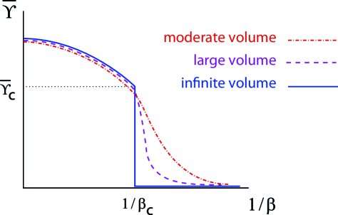
Figure 1: A qualitative picture of the expected coupling dependence of the helicity modulus in different volumes.

In fact, the observations for the standard action [26] and for the step action [24] are compatible with this picture.

We expect the same behaviour for the constraint action, where (in an infinite volume) $\bar{\Upsilon}(\delta)$ should jump to $0$ when $\delta$ exceeds $\delta_{\rm c}$. As a test, we measured $\bar{\Upsilon}(\delta)$ in volumes of size $L=8\dots 64$. Figure 2 shows the results, which are well compatible with this expectation.

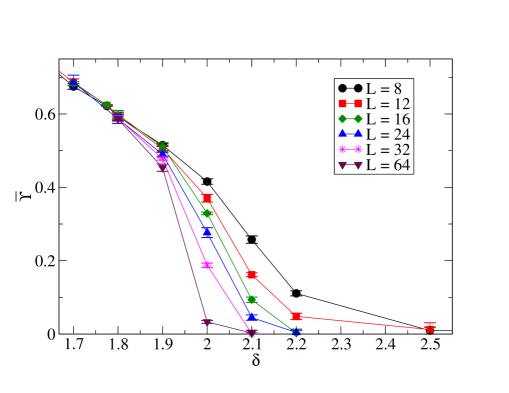
Figure 2: Results for $\bar{\Upsilon}$ in six volumes, over a range of $\delta$ angles, which includes $\delta_{\rm c}\simeq 1.775$. We observe the expected trend towards a jump down to $0$ next to $\delta_{\rm c}$, in analogy to the schematic Figure 1.

To further underscore this observation, Figure 3 shows specifically the values $\bar{\Upsilon}(\delta=2)$ in various volumes, which have a highly plausible extrapolation to $0$ in the thermodynamic limit $L\to\infty$.

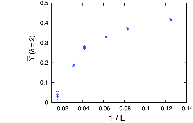
Figure 3: Values of $\bar{\Upsilon}$ at $\delta=2$ against $1/L$. For increasing volume they rapidly drop towards $0$, in agreement with the helicity gap picture.

2.4 Critical value of the helicity modulus

We now focus on the critical constraint angle given in Ref. [16] (cf. Section 1), $\delta_{\rm c}=1.77521$, and measure $\bar{\Upsilon}_{\rm c}$ in various volumes. We simulated the model on $L\times L$ lattices in the range $L=8\dots 256$ with dynamical boundary conditions. Figure 4 shows two of our histograms for the twist angles $\alpha$. The histograms for $L\leq 128$ are based on more than a million $\alpha$ values, see Table 1.

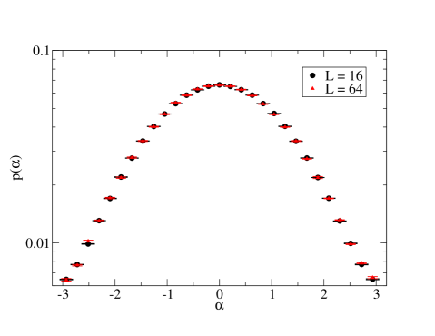
Figure 4: Histograms for the twist angle $\alpha$, measured by heat bath simulations in various volumes. A fit in some interval $[-\alpha_{0},\ \alpha_{0}]$ ($\alpha_{0}=(n_{\rm bin}-1)\cdot\pi/30$) determines the curvature in the maximum at $\alpha=0$.

The optimal evaluation of the curvature at $\alpha=0$ was identified by probing a variety of bin sizes, and fitting ranges. The best option (regarding the ratio $\chi^{2}$/d.o.f.) involves 31 bins for the $\alpha$ values. A parabolic fit is performed by including the number $n_{\rm bin}$ of bins around $\alpha=0$, which again minimises the quantity $\chi^{2}$/d.o.f. Table 1 displays this number for each volume, along with our results for $\bar{\Upsilon}_{\rm c}$ and their uncertainties.

$L$	statistics	$n_{\rm bin}$	$\chi^{2}$/d.o.f.	$\bar{\Upsilon}_{\rm c}$	error
8	16 097 744	21	0.000004	0.6217	0.0006
12	9 142 032	17	0.000004	0.6234	0.0011
16	6 266 902	15	0.000005	0.6243	0.0015
32	2 506 795	13	0.000006	0.6257	0.0025
64	1 001 355	13	0.000016	0.6355	0.0041
128	1 2417 90	7	0.000010	0.6345	0.0041
256	584 178	7	0.000020	0.6333	0.0073

Table 1: Numerical results for the dimensionless helicity modulus, measured at the critical constraint angle $\delta_{\rm c}$, in $L\times L$ volumes, by means of histograms for the twist angles $\alpha$ (the statistics gives the number of $\alpha$ values involved).

For all sizes $L$ that we consider, the deviations of $\bar{\Upsilon}_{\rm c}$ from the theoretical value $\bar{\Upsilon}_{\rm c,\,theory}$ in eq. (2.3) is less than $2.4\ \%$, and for $L\geq 64$ our results confirm the prediction within the errors. This observation is highly remarkable in view of earlier attempts to measure $\bar{\Upsilon}_{\rm c}$ with other lattice actions, which could only claim agreement with the BTK value based on specific large volume extrapolations. For illustration, Figure 5 compares our results to those for the standard action [12] and for the step action [24].

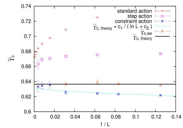
Figure 5: Numerical results for $\bar{\Upsilon}_{\rm c}$ on $L\times L$ lattices at the critical parameter, for the standard action (data from Ref. [12]), the step action (data from Ref. [24]) and for the constraint action (data from Table 1). In the former two cases, all measured results differ significantly from the theoretical BKT value $\bar{\Upsilon}_{\rm c,\,theory}$ in eq. (2.3), which could only be attained with extended extrapolations. Only for the constraint action the results agree with the BKT prediction for $L\geq 64$, and the deviation is just $1.9\ \%$ ($2.3\ \%$) even at $L=16$ ($L=8$). For that action, we show the fit to eq. (2.4) with $c_{1}=-0.0335382$, $c_{2}=0.166499$. (We also include data measured at $\delta_{\rm c,sw}=1.756$, denoted as $\bar{\Upsilon}_{\rm c,sw}$, which will be discussed in Subsection 3.1.)

The fit for the constraint action data to eq. (2.4) yields

$$c_{1}=-0.034(11)\ ,\quad c_{2}=0.17(80)\ .$$ (2.8)

The corresponding graph is included in Figure 5.

Thus there is a clear discrepancy from the $c_{1}$ value in eq. (2.5), which was derived in the spin wave limit and with renormalisation group considerations. Of course, there is no rigorous guarantee that our data really reveal the asymptotic large $L$ behaviour, although this is what one would naturally expect.

Still, this discrepancy may look surprising, and it calls for a discussion. On the other hand, this observation might be viewed in light of the recent experience with topological (and mixed) lattice actions:

• Based on the mapping of the 2d XY model onto the sine-Gordon model, Ref. [27] derived — in addition to the continuum Step Scaling Function [13] — the coefficient of the leading lattice artifact term, which was also assumed to be universal. In fact, it agrees with data for the standard action [14], but it clearly disagrees with results for various topological actions, including the constraint action [16].

• In the large $N$ limit of the 2d O(N) model, there are corrections to the continuum Step Scaling Functions, which start in the quadratic order of the lattice spacing, multiplied by some logarithmic factor. In this case, even the leading power of this logarithmic term differs between the standard action and topological actions [28].

• For the 2d O(3) model with a “mixed action” (with a standard coupling plus an angular constraint), the Step Scaling Function has lattice artifacts, which seem incompatible with the expected asymptotic agreement with the standard action artifacts [28].

• For the 1d O(2) model (the quantum rotor), the topological actions are plagued by linear lattice artifacts [15], although one might expect them to be generically quadratic. (However, since this is not a field theoretic example, universality arguments do not apply.)

Nevertheless, in the next section we are going to investigate further the applicability of spin wave predictions to the constraint action results, now proceeding to much larger lattices.

3 Binder cumulant and second moment correlation length

For the measurement of the dimensionless helicity modulus $\bar{\Upsilon}$ we were restricted to use the heat bath algorithm described in Appendix A. Therefore the lattice sizes which could be reached were rather moderate ($L\leq 256$). In this range, the results agree with the thermodynamic prediction for $\bar{\Upsilon}_{\rm c,theory}$, but not with the prediction for the coefficient $c_{1}$.

For an extended test of the applicability of spin wave theory predictions, we now consider the Binder cumulant $U_{4}$ and the second moment correlation length $\xi_{2}$. This can be done at fixed periodic boundary conditions, hence we can apply the more efficient Wolff cluster algorithm [29] and explore much larger lattices.

We start from the magnetisation $\vec{m}$ and the magnetic susceptibility $\chi$,

$$\vec{m}=\sum_{x}\vec{e}_{x}\quad,\quad\chi=\frac{1}{L^{2}}\langle\vec{m}^{2}\rangle\ .$$ (3.1)

The Binder cumulant $U_{4}$ is obtained as

$$U_{4}=\frac{\langle(\vec{m}^{2})^{2}\rangle}{\langle\vec{m}^{2}\rangle^{2}}\ .$$ (3.2)

To compute the second moment correlation length $\xi_{2}$, one considers the Fourier transform of the correlation function $G(x-y)=\langle\vec{e}_{x}\cdot\vec{e}_{y}\rangle$

$$\widetilde{G}(p)=\sum_{x}G(x)\exp({\rm i}px)\ ,$$ (3.3)

on an $L\times L$ lattice. It contains the magnetic susceptibility $\chi=\widetilde{G}(p=0)$, as well as the quantity $F=\widetilde{G}(p=(2\pi/L,0))$ at the smallest non-vanishing momentum. The second moment correlation length is given by

$$\xi_{2}=\frac{1}{2\sin(\pi/L)}\left(\frac{\chi}{F}-1\right)^{1/2}\ .$$ (3.4)

It is very similar to the (actual) correlation length, but easier to measure.

Predictions for $U_{4}$ [30] and $\xi_{2}/L$ [12] in the thermodynamic limit $L\to\infty$ of the 2d XY model have been calculated by using the spin wave approximation, which yields

$$U_{4,{\rm sw}} = 1.018192(6)+\frac{C_{1}}{\ln L+C_{2}}+\dots\ ,$$

$$\xi_{2,{\rm sw}}/L = 0.7506912\dots+\frac{C_{1}{{}^{\prime}}}{\ln L+C_{2}{{}^{\prime}}}+\dots\ ,$$ (3.5)

where $C_{1},\,C_{2},\,C_{1}{{}^{\prime}},C_{2}{{}^{\prime}}$ are constants. These asymptotic values, and the coefficients $C_{1}$, $C_{1}{{}^{\prime}}$ are interesting in view of universality. Ref. [30] obtained results for the standard action of the 2d XY model, which are consistent with two other models in the same universality class, over a wide range of sizes $L$.

We computed $U_{4}$ and $\xi_{2}/L$ for the constraint action, as well as the standard action, at the critical parameter, on $L\times L$ lattices in the range $L=12\dots 1024$. Our results for the standard action (at $\beta_{\rm c}=1.1199$) fully agree with those obtained by Hasenbusch [30]. Figure 6 shows our results for the Binder cumulant. For both lattice actions we observe a trend to a plateau value, which is close to the prediction (3.5), but not in exact agreement. There remains a deviation of about 1 per mille, which is positive (negative) for the constraint action (standard action).

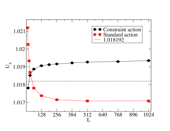
Figure 6: The Binder cumulant for the constraint action and for the standard action, compared to the spin wave prediction in the large volume limit.

The behaviour of the ratio $\xi_{2}/L$ is qualitatively similar, as Figure 7 shows. Here we observe a deviation from the spin wave prediction (3.5) on the percent level, again with opposite signs for the two actions. This time the data for the constraint action are clearly closer to the prediction. Our numerical values for $U_{4}$ and $\xi_{2}/L$ are listed in Tables 2 and 3.

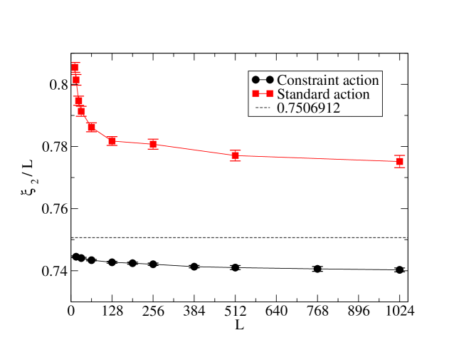
Figure 7: The second moment correlation length $\xi_{2}$, divided by the lattice size $L$, for the standard action and for the constraint action. The results for both actions deviate a little from the spin wave prediction.

$L$	$U_{4}$	$\xi_{2}/L$
16	1.017811(5)	0.7445(3)
32	1.018521(6)	0.7441(3)
64	1.018871(7)	0.7434(3)
128	1.019061(8)	0.7427(4)
192	1.019121(9)	0.7424(4)
256	1.01916(7)	0.7421(4)
384	1.019218(9)	0.7413(4)
512	1.019266(6)	0.7410(7)
768	1.019294(13)	0.7406(8)
1024	1.01935(21)	0.7402(7)

Table 2: Numerical results for $U_{4}$ and $\xi_{2}/L$, obtained with the constraint action.

$L$	$U_{4}$	$\xi_{2}/L$
12	1.02119(4)	0.8054(17)
16	1.02025(5)	0.8014(18)
24	1.01933(4)	0.7947(15)
32	1.01868(6)	0.7913(18)
64	1.01780(4)	0.7861(15)
128	1.01738(2)	0.7817(15)
256	1.01715(3)	0.7807(17)
512	1.01708(3)	0.7771(18)
1024	1.01708(2)	0.7751(21)

Table 3: Numerical results for $U_{4}$ and $\xi_{2}/L$, obtained with the standard action.

Considering the stable behaviour on the largest lattice sizes that we explored, and the even larger lattices where Hasenbusch simulated the standard action [30], it is not obvious to expect that both curves would ultimately converge to the predicted values for $L\to\infty$, even in the presence of logarithmic finite size effects. Hasenbusch suspected that (universal) sub-leading finite $L$ corrections to the spin wave results could explain this discrepancy. However, this scenario has now the additional difficulty to explain our observation that the results for different lattice actions disagree as well.

For the standard action, Hasenbusch estimated a minimum of $U_{4}$ around $L\approx 6200$, and an extremely slow increase on even larger lattices. Of course, this scenario — and its analogue for the constraint action with a $U_{4}$ maximum in some huge volume — cannot be excluded. The alternative scenario would be that $U_{4}$ and $\xi_{2}/L$ are not truly (but still approximately) universal quantities. It remains as an open question if that alternative scenario holds, and how it could possibly be explained.

3.1 Criticality determined from spin wave predictions

For lattice sizes in the range up to $L=1024$, we have seen in Figures 6 and 7, as well as Table 2 and 3, small but significant discrepancies from the spin wave predictions for the quantities $U_{4}$ and $\xi_{2}/L$. In this subsection we are going to explore an alternative approach, which takes these predictions as a basis to determine the critical point. Hence in this alternative approach we assume the predictions (3.5) to be correct, and the numerical data to display a visible convergence towards these values for the lattice sizes under consideration.

For the constraint action this leads to an alternative suggestion for the critical angle, which amounts to

$$\delta_{\rm c,sw}=1.756(2)\ .$$ (3.6)

The results for $U_{4}$ and $\xi_{2}/L$ at this angle are shown in Figure 8. Indeed this shift from $\delta_{\rm c}$ to $\delta_{\rm c,sw}$ provides convincing convergence of both quantities towards the spin wave predictions.

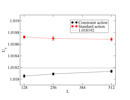
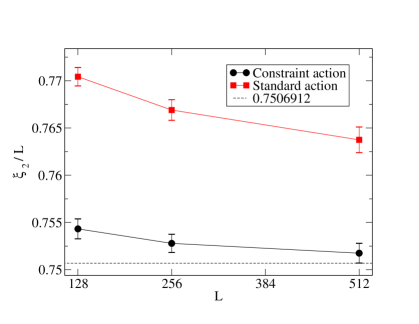
Figure 8: The Binder cumulant $U_{4}$ and the ratio $\xi_{2}/L$ at the alternative suggestions for the critical parameters, based on the spin wave predictions: $\delta_{\rm c,sw}=1.756$ (for the constraint action) and $\beta_{\rm c,sw}=1.112$ (for the standard action).

Next we measured $\bar{\Upsilon}$ at $\delta_{\rm c,sw}$ to verify if the curve $\bar{\Upsilon}_{\rm c,sw}(L)$ also converges to the predicted value $\bar{\Upsilon}_{\rm c,theory}$ in the thermodynamics limit. These data points are included in Figure 5. They do converge to $\bar{\Upsilon}_{\rm c,theory}$, which is already attained (within errors) at $L=12$. So to this point $\delta_{\rm c,sw}$ looks like a plausible alternative for the critical constraint angle.

However, if we fit these data to the predicted asymptotic formula (2.4) we obtain

$$c_{1}=0.00015(12)\ ,\quad c_{2}=-2.19(9)\ ,$$ (3.7)

so the discrepancy from the $c_{1}$ prediction (2.5) persists. In fact the determination of $\delta_{\rm c}$ from $\xi$ is somewhat involved, but even if we shift this value considerably, the absolute value $|c_{1}|$ — as obtained from our fits — remains tiny and incompatible with $\approx 0.32$. Of course we cannot rigorously rule out that the use of tremendously large volumes and ultra-high precision would still provide that value. However, the results accessible with a reasonable computational effort can hardly be reconciled with the $c_{1}$ prediction, even with some tolerance for the critical $\delta$ angle.

In order to explore the alternative approach of this subsection further, we tried the same method also for the standard action. However, in this case it is not possible to find any $\beta$ parameter which would lead to good convergence of $U_{4}$ and of $\xi_{2}/L$ towards the the values in eq. (3.5). As a compromise we choose $\beta_{\rm c,sw}=1.112$; a separate matching of $U_{4}$ (of $\xi_{2}/L$) would suggest a larger (lower) $\beta$, as Figure 8 shows. Moreover, $\beta_{\rm c,sw}$ is incompatible with the value that we quoted earlier in Section 1, $\beta_{\rm c}=1.1199(1)$ [8], which is based on a careful high precision study, and which is accepted in the literature.

Therefore we consider the critical parameter evaluated from the correlation length $\xi$ more reliable. As a further cross-check, we fit the formula

$$\xi\propto\exp\Big{(}{\rm const.}/(\delta-\delta_{\rm c}^{\rm(t)})^{\nu_{\rm c}}\Big{)}$$ (3.8)

to our data for the correlation length $\xi$ at $\delta=1.89\dots 2$. Now we insert some trial value for $\delta_{\rm c}^{(t)}$ and evaluate the critical exponent $\nu_{\rm c}$ through the fit. In particular, if we insert $\delta_{\rm c}^{\rm(t)}=\delta_{\rm c}=1.77521$ or $\delta_{\rm c}^{\rm(t)}=\delta_{\rm c,sw}=1.756$, we obtain $\nu_{\rm c}=0.501(7)$ and $0.691(7)$, respectively. The corresponding extrapolations in $\xi(\delta)$ are shown in Figure 9 (above). The plot below illustrates the results for $\nu_{\rm c}$ obtained in this way (along with its error band) over the entire range $\delta_{\rm c}^{\rm(t)}=1.75\dots 1.78$. The BKT value $\nu_{\rm c}=1/2$ [11] singles out $1.7748<\delta_{\rm c}<1.7763$, which is clearly incompatible with $\delta_{\rm c,sw}$.

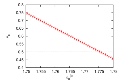
Figure 9: On top: The correlation length $\xi$, measured in large volumes (up to convergence in $L$ at fixed $\delta$) and its fits to the function (3.8) for $\delta_{\rm c}^{\rm(t)}=\delta_{\rm c}=1.77521$ and for $\delta_{\rm c}^{\rm(t)}=\delta_{\rm c,sw}=1.756$. Below: The critical exponent $\nu_{\rm c}$, obtained by fits to eq. (3.8), as a function of the angle inserted for $\delta_{\rm c}^{\rm(t)}$. We see that $\delta_{\rm c}^{(t)}\in[1.7748,1.7763]$ leads to agreement with the theoretically predicted exponent $\nu_{\rm c}=1/2$ [11], in contrast to $\delta_{\rm c,sw}$.

4 Free vortices and vortex–anti-vortex pairs

We define the relative angle between nearest neighbour spins with a ${\rm mod}~{}2\pi$ operation, which acts such that the absolute value becomes minimal,

$$\Delta\Phi_{x,y}=(\Phi_{x}-\Phi_{y})\ {\rm mod}\ 2\pi\in(-\pi,\pi]\ .$$ (4.1)

If we sum these relative angles over the corners $x,y,z,w$ of a plaquette, and normalise by $2\pi$, we obtain the vortex number

$$v_{\Box}=\frac{1}{2\pi}(\Delta_{x,y}+\Delta_{y,z}+\Delta_{z,w}+\Delta_{w,x})\in\{1,0,-1\}\ .$$ (4.2)

For $v_{\Box}=1$ ($v_{\Box}=-1$) the plaquette carries a vortex (an anti-vortex); higher vortex numbers ($|v_{\Box}|>1$) do not occur.

As in the previous section we deal with periodic boundary conditions. Hence Stokes’ Theorem implies that the total vorticity always vanishes,

$$\sum_{\Box}v_{\Box}=0\ .$$ (4.3)

With this terminology, the picture of vortex (un)binding as the mechanism that drives the BKT transition can be probed explicitly. For the standard action (1.2) this has been done in Refs. [31, 32, 33, 34], and the results are essentially consistent with the suggested picture. These considerations were static, comparing the behaviour in the different phases.

There are also studies of the dynamics of the unbinding when $\beta$ decreases gradually below $\beta_{\rm c}$. Such considerations proceeded first by solving the Fokker-Planck equation [35], and later by Monte Carlo simulations [36]. For the standard action, the outcome was again compatible with the picture of dissociating vortex–anti-vortex pairs.

For the constraint action that we are investigating here, we first show in Table 4 and Figure 10 how the total vortex plus anti-vortex density $\rho$ depends on $\delta$. Vortices are possible for $\delta>\pi/2$, but their density become significant only around $\delta\mathop{\raise 1.29167pt\hbox{$>$\kern-7.5pt\raise-4.73611pt\hbox{$\sim$}}}1.9$, i.e. somewhat above $\delta_{\rm c}$.

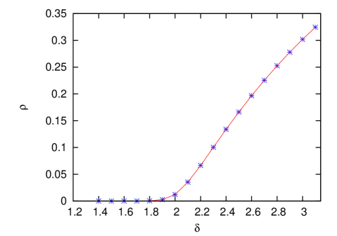
Figure 10: The vortex density $\rho$, i.e. the number of plaquettes with $|v_{\Box}|=1$, divided by the volume. We show results obtained at $L=128$, but the volume dependence is marginal. Error bars are included, but too small to be seen, and the line is drawn to guide the eye.

$\delta$	$\rho$	$\rho_{1}^{\rm free}$	$\rho_{2}^{\rm free}$	$\rho_{4}^{\rm free}$
1.8	0.00032(1)	0.00016(5)	0.000021(7)	0.000013(5)
2	0.0122(1)	0.0068(1)	0.0045(2)	0.0016(1)
2.2	0.066424(7)	0.0334(1)	0.015517(8)	0.00172(1)
2.4	0.13390(5)	0.05527(3)	0.01733(3)	0.00030(1)
2.6	0.19661(2)	0.06701(2)	0.014110(3)	0.000032(1)

Table 4: The density of all vortices (plus anti-vortices), $\rho$, and of the “free vortices” $\rho_{r}^{\rm free}$ — without any opposite partner within Euclidean distance $r=1$, $2$ or $4$ — at different constraint angles $\delta$. The measurement was performed at $L=128$, but the size dependence is modest.

As an illustration, we show in Figure 11 the vortex and anti-vortex distribution in typical configurations of a $L=64$ lattice at $\delta=1.85$, $2$, $2.15$ and $2.3$. We observe also here the increase in the total vortex density. In addition we recognise a strong trend towards vortex–anti-vortex pair formations at $\delta=1.85$, which fades away for increasing $\delta$. These specific configurations appear qualitatively consistent with the (un)binding mechanism. However, a solid verification requires statistical investigations, which we will present in the rest of this section.

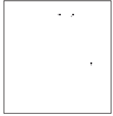
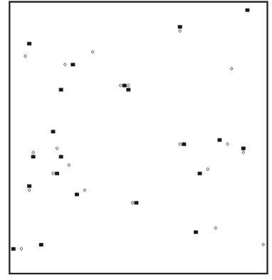
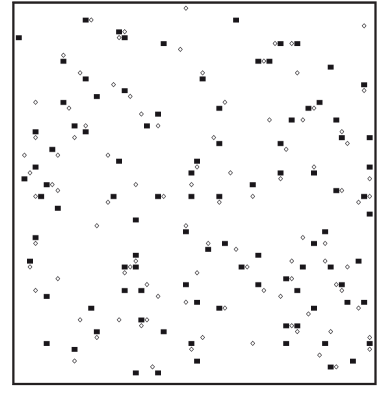
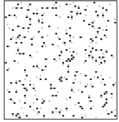
Figure 11: The distribution of vortices (filled squares) and anti-vortices (empty diamonds) in typical configurations on a $64\times 64$ lattice at $\delta=1.85$, $2$ (above), and $\delta=2.15$, $2.3$ (below). For growing $\delta$ we observe an increasing vortex density (cf. Figure 10), but a decreasing trend towards vortex–anti-vortex pair formations, and therefore more and more free vortices (cf. Figure 12).

4.1 Free vortex density

According to the established picture, it is not the total vortex density which matters for the fate of a long-ranged order, but rather the density of “free vortices”. There is clearly some ambiguity in an explicit definition of this term. An obvious possibility is to count those vortices which are not accompanied by any anti-vortex (or vice versa) within some Euclidean distance $r$. Table 4 and Figure 12 show the corresponding free vortex densities $\rho_{r}^{\rm free}$ for $r=1$, $r=2$ and $r=4$. In all cases, there is a significant onset in the interval $\delta=1.8\dots 1.9$, which is compatible with the onset of $\rho$. For $r\geq 2$ the densities $\rho_{r}^{\rm free}$ decrease again at large $\delta$ angles, as a consequence of the high total density $\rho$. However, it is the first onset which indicates the dissociation of vortex–anti-vortex pairs, and which is therefore relevant for the BKT picture. Our observation is compatible with this picture, up to a shift of the onset somewhat into the massive phase. A similar behaviour has been observed for the standard action [31, 32, 33, 34].

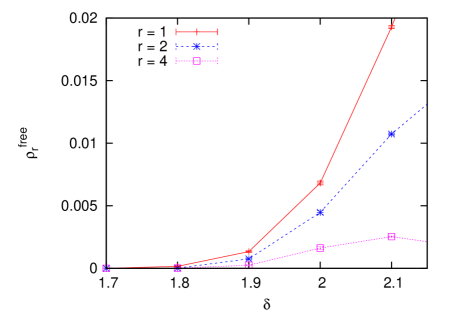
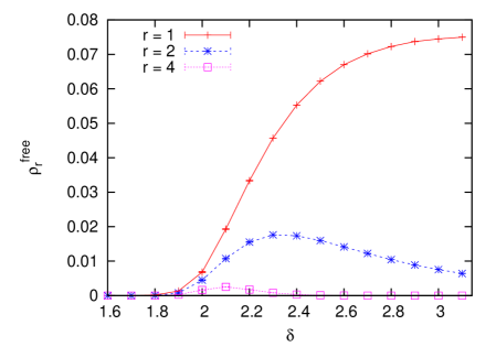
Figure 12: The density of “free vortices”, $\rho_{r}^{\rm free}$, i.e. vortices or anti-vortices, which do not have an opposite partner within some Euclidean distance $r$. For various choices of $r$, a significant density sets in around $\delta=1.8\dots 1.9$. This is best seen from the plot above, while the plot below provides an overview. These results are obtained at $L=128$, but they are hardly size dependent.

4.2 Vorticity correlation

The established picture of the BKT transition also implies a sizable vorticity anti-correlation over short distances in the massless phase — in particular over distance $1$. Figure 13 shows results for the vorticity correlation function

$$C(r)=\langle\,v_{\Box,(x_{1},x_{2})}\,v_{\Box,(x_{1}+r,x_{2})}\,\rangle|_{|v_{\Box,(x_{1},x_{2})}|=1}$$ (4.4)

over distances $r=1$, 2 and 3, at a set of constraint angles $\delta\geq\delta_{\rm c}$. Indeed we confirm a marked anti-correlation over distance 1 around $\delta_{\rm c}$, which rapidly fades away when $\delta$ increases.

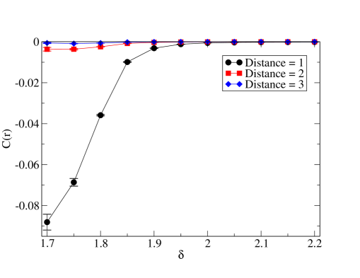
Figure 13: The vorticity correlation function $C(r)$ of eq. (4.4) over distances $r=1,2,3$, as a function of the constraint angle $\delta$. In particular, there is a strong anti-correlation over the minimal distance $r=1$ at $\delta\mathop{\raise 1.29167pt\hbox{$<$\kern-7.5pt\raise-4.73611pt\hbox{$\sim$}}}\delta_{\rm c}$, in agreement with the formation of vortex–anti-vortex pairs. This effect get lost rapidly as $\delta$ increases, since the pairs tend to dissociate.

Of course, there is a trivial argument for $C(1)<0$, since the relative angle of the common link of adjacent plaquettes contributes to their vorticity with opposite sign. However, this alone does not explain the sharp slope at $\delta=1.8\dots 1.9$, and the remaining anti-correlation at $r=2$ and $3$.

This observation is reminiscent of the anti-correlation of the topological charge density in gauge theories, for configurations in the neutral sector [38]. This property was confirmed explicitly on the lattice for QCD [39] and for the Schwinger model [40].

4.3 Vortex–anti-vortex pair formation

Finally we want to investigate the vortex–anti-vortex pair formation from yet another, more direct perspective. Given a configuration, we first identify its $N$ vortices and $N$ anti-vortices, and we search for the optimal pairing. This optimisation minimises the quantity

$$D^{2}=\frac{1}{N}\,\sum_{i=1}^{N}d_{{\rm VA},\,i}^{\,2}\ \,,$$ (4.5)

where $d_{{\rm VA},\,i}$ are the Euclidean distances that separate the vortex–anti-vortex partners. The straightforward method of checking all possibilities is safe, but only applicable up to $N\approx 14$. We work again at lattice size $L=128$ with constraint angles up to $\delta=2.05$, where typically $N$ is close to $200$ (see Figure 10). In order to still identify the optimal pairing (with high probability), we applied the technique of “simulated annealing”, see Appendix C.

The results for $D^{2}$ at different angles $\delta$ are shown in Figure 14. We see a slight increase at $\delta\mathop{\raise 1.29167pt\hbox{$>$\kern-7.5pt\raise-4.73611pt\hbox{$\sim$}}}1.8$, followed by a sharp increase at $\delta\mathop{\raise 1.29167pt\hbox{$>$\kern-7.5pt\raise-4.73611pt\hbox{$\sim$}}}1.9$. This is another piece of evidence for the (un)binding mechanism behind the BTK transition, and once more the obvious effect is shifted somewhat into the massless phase.

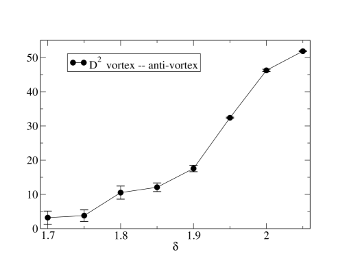
Figure 14: The mean distance squared within the vortex–anti-vortex pairs, $D^{2}$, on a $L=128$ lattice. The significant (drastic) increase above $\delta_{\rm c}$ (above $\delta=1.9$) indicates the unbinding of some (numerous) pairs.

To take a closer look at the meaning of the $D^{2}$ values in Figure 14, we add the following comparison: we take the mean vortex number $N$ at some $\delta$ angle, and spread the same number of $N$ vortices and anti-vortices randomly (with a flat probability) over the $L=128$ lattice. Figure 15 (above) compares the $D^{2}$ values obtained in this way to those of the simulation. We see a large difference, i.e. a strong trend towards non-accidental pair formation in the simulation, in particular up to $N\approx 50$, which corresponds to $\delta\approx 1.9$ in the simulation; for larger $N$ this trend is much weaker.

As a further reference quantity, we add (at even $N$) the same comparison for

$$R_{\rm VV}^{2}=\frac{2}{N}\,\sum_{i=1}^{N/2}d_{{\rm VV},\,i}^{\,2}\quad{\rm and}\quad R_{\rm AA}^{2}=\frac{2}{N}\,\sum_{i=1}^{N/2}d_{{\rm AA},\,i}^{\,2}\ ,$$ (4.6)

where $d_{{\rm VV},\,i}$ ($d_{{\rm AA},\,i}$) are the distances between two vortices (two anti-vortices), if we perform the pairing which minimises $R_{\rm VV}^{2}$ ($R_{\rm AA}^{2}$). This process is somewhat different from the case of opposite pairs (there are only $(N-1)!!$ possibilities). Figure 15 (below) shows that for these quantities (which statistically coincide) it makes hardly any difference if we take simulated or random distributed vortices (and anti-vortices). Hence the trend for pair formations is in fact specific to the pairs of opposite partners.

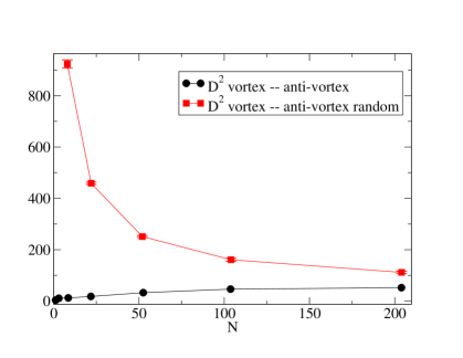
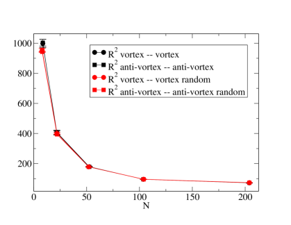
Figure 15: The quantities $D^{2}$ (above), $R_{\rm VV}^{2}$ and $R_{\rm AA}^{2}$ (below) of eqs. (4.5), (4.6). In each case, we compare the values for simulated configurations (at a $\delta$ angle, which leads on average to $N$ vortices) to $N$ randomly distributed vortices and anti-vortices. For $D^{2}$ this makes a sizable difference, in particular at low $\delta$, due to the pair formation. On the other hand, such a formation mechanism does not exist for vortex–vortex pairs, or anti-vortex–anti-vortex pairs, as the results for $R_{\rm VV}^{2}$ and $R_{\rm AA}^{2}$ reveal.

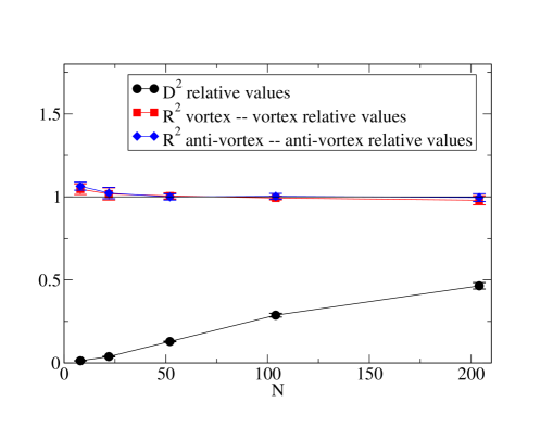
Figure 16: The ratio between the quantities $D^{2}$, $R_{\rm VV}^{2}$ and $R_{\rm AA}^{2}$ for simulated configurations, and for random distributions, with $N$ vortices and $N$ anti-vortices.

For an ultimate clarification, Figure 16 shows the ratios between $D^{2}$ for simulated configurations with $N$ vortices and $N$ anti-vortices, and with the same number of randomly distributed vortices and anti-vortices. We see again the powerful trend towards pair formation at small $N$, which fades away as $N$ increases. The plots also shows the corresponding ratios for $R_{\rm VV}^{2}$ and for $R_{\rm AA}^{2}$. In those cases the difference between simulation and random distribution is tiny; for small $N$ (corresponding to $\delta\mathop{\raise 1.29167pt\hbox{$<$\kern-7.5pt\raise-4.73611pt\hbox{$\sim$}}}1.9$) we even observe a slight trend of repulsion between simulated vortices.

5 Conclusions

We have investigated the phase transition of the 2d XY model in the formulation with the constraint lattice action (1.5). Simulations with dynamical boundary conditions confirmed — in an unprecedented manner — the value of the dimensionless helicity modulus $\bar{\Upsilon}_{\rm c,\,theory}$, which was predicted for a BKT phase transition. In contrast to other lattice actions, the finite size effects are modest in this case. In particular, the value of $\bar{\Upsilon}_{\rm c}$ remains close to the BKT value, up to $1.9~{}\%$ down to volumes as small as $16\times 16$.

This eliminates any doubt that the constraint lattice action does belong to the same universality class as the conventional lattice actions, which involve spin couplings, like the standard action (1.2). Moreover, this provides one of the most compelling numerical evidences that has ever been found for the BKT behaviour of the 2d XY model.

Regarding the spin wave predictions for this model, however, we observed discrepancies in the range of lattice sizes that we could explore. This is seen clearly for the coefficient $c_{1}$ in the leading finite size correction to $\bar{\Upsilon}_{\rm c,\,theory}$, cf. eq. (2.4), although the universality of $c_{1}$ is also supported by renormalization group flow arguments [23]. In this context, however, our data are restricted to $L\leq 256$.

On much larger lattices we still observed small but significant deviations from the values predicted by spin wave theory for $U_{4}$ and $\xi_{2}/L$. In this case there are also deviations for the standard action, at least up to the largest volumes that have been simulated. For both quantities, the data obtained for the two actions deviate from the spin wave prediction with opposite signs.

For the constraint action there is an alternative angle $\delta_{\rm c,sw}$, which leads to good agreement with the spin wave predictions for $U_{4}$ and $\xi_{2}/L$. However, adopting that value does still not fix the discrepancy with the prediction for the coefficient $c_{1}$. In addition it is not compatible with our data for the correlation length $\xi$, and this approach to determine the critical point does not work well for the standard action.

Finally we verified the picture of vortex–anti-vortex pair (un)binding as the mechanism behind the BKT transition. Our results for the density of free vortices and anti-vortices (without an opposite partner up to some distance), for the vorticity correlation, and for the sum over pair separations squared, are all compatible with this picture. As for the conventional actions, we can indeed confirm that a relevant number of pairs dissociate when we move from the massless to the massive phase, so that the free vortex density becomes significant. However, this consideration alone would not enable a precise determination of the critical constraint angle $\delta_{\rm c}$, in analogy to the standard action, where the critical value $\beta_{\rm c}$ could only be estimated approximately based on the pair (un)binding. In both cases, the obvious onset of the free vortex density is shifted somewhat into the massive phase.

The validity of this mechanism is highly non-trivial, since the free vortices do not cost any energy (if the constraint allows them). Hence their suppression in the range $\pi/2<\delta\mathop{\raise 1.29167pt\hbox{$<$\kern-7.5pt\raise-4.73611pt\hbox{$\sim$}}}\delta_{\rm c}$ can only be explained by the combinatorial frequency of configurations carrying different vorticities. In this regard, our results deviate from the established point of view, since they demonstrate that a BKT transition can occur even without any Boltzmann factor suppression of free vortices.

To summarise, the quantitative BKT prediction for the helicity modulus in the thermodynamic limit is confirmed excellently, and the picture behind it as well. On the other hand, the inspiration of this picture — with a Boltzmann weight for free vortices — is not confirmed, since we observe the same feature on purely combinatorial grounds.

Acknowledgements: Michael Bögli has contributed to this work at an early stage. We thank him in particular for providing the data that we used in Figure 9. We further thank Uwe-Jens Wiese for instructive discussions, and Martin Hasenbusch and Ulli Wolff for interesting remarks.

This work was supported by the Mexican Consejo Nacional de Ciencia y Tecnología (CONACyT) through project 155905/10 “Física de Partículas por medio de Simulaciones Numéricas” and through the scholarship 312631 for graduate studies, as well as DGAPA-UNAM. The simulations were performed on the cluster of the Instituto de Ciencias Nucleares, UNAM. We thank Luciano Díaz and Enrique Palacios for technical support.

Appendix A Heat bath algorithm

When we run a Metropolis algorithm for the constraint action given in eq. (1.5), the decision about accepting a proposed update step is fully deterministic: if the updated configuration obeys the constraint, it will always be accepted, otherwise it must be rejected. This unusual property holds both for updated spin variables and — in case of dynamical boundary conditions — also for the updated twist angle $\alpha$.

In this algorithmic scheme it is optimal to update the spins one by one. If we suggest a new spin

$$\vec{e}_{x}=\left(\begin{array}[]{c}\cos\phi_{x}\\ \sin\phi_{x}\end{array}\right)\to\vec{e}_{x}{\,{}^{\prime}}=\left(\begin{array}[]{c}\cos\phi_{x}{{}^{\prime}}\\ \sin\phi_{x}{{}^{\prime}}\end{array}\right)\ ,$$ (A.1)

it depends on its four nearest neighbours if it will be accepted, and — if $x$ is next to the twisted boundary — also on $\alpha$. The common Metropolis implementation would suggest a new angle in some small interval around the previous one, $\phi_{x}{{}^{\prime}}\in[\phi_{x}-\Delta,\phi_{x}+\Delta]$.

It is noteworthy, however, that for $\delta>\pi/2$ (the case we are dealing with) the allowed circular section for $\phi_{x}{{}^{\prime}}$ may consist of disjoint arcs. Hence by using a small $\Delta$, one could overlook part of these allowed arcs, far away from $\phi_{x}$, although those angles are not suppressed. Therefore it is better to probe the entire allowed circular section, and choose $\phi_{x}{{}^{\prime}}$ therein with flat probability. The situation is similar for the update of the twist angle $\alpha\to\alpha^{\prime}$, which should also be chosen arbitrarily in the allowed circular section (which does not violate the constraint).

Thus the new values do not depend on the previous ones, but only on (part of) the rest of the configuration, so this is a heat bath algorithm. This algorithm is robust and generally applicable for this type of actions. It was also used for quenched QCD simulations with an analogous constraint [41], i.e. a lower bound for each plaquette variable (which was in that case combined with a kinetic term).

One could compute the boundaries of the allowed section, including possible disjoint pieces, but in particular in the case of $\alpha^{\prime}$ this tends to be tedious. A simpler method suggests a new angle, $\phi_{x}{{}^{\prime}}$ or $\alpha^{\prime}$, anywhere on the circle (with flat probability), and checks if it is allowed. If not, one tries again and repeats this until one finds an allowed one — this is a multi-hit procedure. In practice one may also limit the number of proposals (“hits”) for the angle under consideration; if it is still not accepted after some maximal number of attempts, one moves on to the update of another angle.

For spin updates and $\delta\approx\delta_{\rm c}$, in average 2 proposals for $\phi_{x}{{}^{\prime}}$ are sufficient. More delicate is the search for an acceptable $\alpha^{\prime}$; here the required hit number is much larger and it increases with the lattice size $L$. At $\delta_{\rm c}$ it takes on average $23.44(4)$ hits for $L=16$, $109(4)$ hits for $L=128$, and $162(5)$ hits for $L=256$. Still, for the study of the helicity modulus the fluctuation of $\alpha$ is vital, so we have to make sure to choose the cutoff for the number of $\alpha^{\prime}$ hits large enough to keep the twist angle moving frequently.

Appendix B Cluster algorithm

Sections 3 and 4 deal with periodic boundary conditions, where it is straightforward and profitable to apply the Wolff cluster algorithm [29]. For a given spin configuration we choose a random Wolff direction $\vec{r}$, which defines a spin flip as a reflection on the line through $0$, which is vertical to $\vec{r}$. We then consider pairs of nearest neighbour spins: if the flip of one of them would violate the $\delta$-constraint, we connect them by a bond. Similar to Appendix A, we encounter the peculiarity that the bonds are set in a fully deterministic way. A set of spins connected by bonds constitutes one cluster. Thus we can divide the whole lattice into clusters (sets of spins, which can only be flipped collectively) and flip each one with probability $1/2$ (multi-cluster algorithm), or we start from a random site and build one cluster, which will be flipped for sure (single-cluster algorithm). In either case, it is guaranteed that the new configuration obeys the $\delta$-constraint, since the collective flip of two spins in the same cluster just changes the sign in their relative angle,

$$\Delta\phi_{x,y}\,\rightarrow\,-\Delta\phi_{x,y}\ .$$ (B.1)

This algorithm is far more efficient than the heat bath method, in particular close to $\delta_{\rm c}$.

Hence it is highly motivated to search for a generalised cluster algorithm, which can also be applied in the presence of dynamical boundary conditions, that we are confronted with in Section 2. This issue has been addressed before in Ref. [42], for a setting where the twist is split over the layers of lattice sites, though that algorithm does not apply to all configurations.

In our setting, the difficulty can be seen as follows. Assume that we build clusters of spins by implementing the instruction to put a bond whenever the flip of one spin out of a nearest neighbour pair would be forbidden. However, the actual goal behind this instruction is that clusters can be flipped freely without ever violating the constraint. If we flip a cluster which includes a spin pair across the twisted boundary, its relative angle

$$\Delta\phi_{x_{2}}^{\rm tb}=(\phi_{L,x_{2}}-\phi_{1,x_{2}})\ {\rm mod}\ 2\pi\ ,\quad x_{2}\in\{1,\dots,L\}$$ (B.2)

before the flip obeys

$$|\,(\Delta\phi_{x_{2}}^{\rm tb}+\alpha)\ {\rm mod}\ 2\pi\,|<\delta\ .$$ (B.3)

A cluster flip (in the above sense) only entails the transition $\Delta\phi_{x_{2}}^{\rm tb}\to-\Delta\phi_{x_{2}}^{\rm tb}$, so it is not guaranteed anymore that the constraint still holds.

We could guarantee that for the cluster under consideration if we flip simultaneously the sign of $\alpha$. However, if the cluster does not capture the entire twisted boundary, this sign change could lead to a violation of the constraint for other spin pairs. Hence we are forced to include $\alpha$ in the cluster building. The inclusion of such a non-local variable — which extends in this case over a whole boundary — would be a conceptual novelty.

B.1 Proposal for a cluster algorithm with dynamical boundary conditions

Here we sketch an attempt to construct a cluster algorithm that involves the twist angle $\alpha$, and its shortcomings. We still assume only one twist, at the boundary between $x_{1}=1$ and $L$. Then the constraint across this boundary takes the form (B.3).

We stay with the prescription that a flip of a spin changes the sign of its component parallel to the Wolff direction, while flipping $\alpha$ means

$$\alpha\rightarrow-\alpha\ .$$ (B.4)

Cluster updates alone are not ergodic, since they never change $|\alpha|$. Hence one has to insert intermediate steps which do perform such a change; this is done best by a heat bath $\alpha$-update, as described in Appendix A.

However, the real issue is the formation of the clusters, such that they can be flipped freely while Detailed Balance is guaranteed. The spin part of a cluster grows in the usual way. Once a cluster touches the twisted boundary, i.e. once it incorporates a spin variable $\vec{e}_{1,x_{2}}$ or $\vec{e}_{L,x_{2}}$, it is possible to add $\alpha$ and/or the periodic neighbour spin to this cluster. If this happens for $\alpha$, any spin $\vec{e}_{1,x_{2}{{}^{\prime}}}$ or $\vec{e}_{L,x_{2}{{}^{\prime}}}$ (with $x_{2}{{}^{\prime}}\neq x_{2}$) could further join the cluster. Thus a “cluster” could consist of disconnected patches.

Let us consider two spins $\vec{e}_{1,x_{2}}$ and $\vec{e}_{L,x_{2}}$ (for some $x_{2}$) and the twist angle $\alpha$. We discuss the options to put a bond which ties 2 of these 3 variables, or even a super-bond which captures all the 3, so they all belong to the same cluster. In light of the above flip definition, there are 8 possible constellations: the projection of the spins in the Wolff direction, and the angle $\alpha$, can all be positive or negative. We have also pointed out before that a collective flip of all 3 variables cannot violate the constraint. Hence we restrict our table to the case $\alpha>0$; the rest is determined by the invariance under a collective flip. We distinguish the orientations of the two spins ($\uparrow$ or $\downarrow$ with respect to the Wolff direction) at $\alpha>0$. For each of these 4 options, the action can be $0$ or $+\infty$, so there are $16$ cases, see Table 5.

In each case we specify which among the 3 variables have to be tied by a bond in order to exclude cluster flips that could violate the constraint. These variables are given as the indices of the bond term $B$, where $1$ and $L$ refer to the spins $\vec{e}_{1,x_{2}}$ and $\vec{e}_{L,x_{2}}$, respectively. Also these bonds are set in a fully deterministic manner.

$\vec{e}_{1,x_{2}}$	$\vec{e}_{L,x_{2}}$	$\exp(-S)$
$\uparrow$	$\uparrow$	$1$	$1$	$1$	$1$	$0$	$1$	$1$	$0$
$\uparrow$	$\downarrow$	$1$	$1$	$1$	$0$	$1$	$1$	$0$	$1$
$\downarrow$	$\uparrow$	$1$	$1$	$0$	$1$	$1$	$0$	$1$	$1$
$\downarrow$	$\downarrow$	$1$	$0$	$1$	$1$	$1$	$0$	$0$	$0$
case number		1	2	3	4	5	6	7	8
bond		—	$B_{1L\alpha}$	$B_{1L\alpha}$	$B_{1L\alpha}$	$B_{1L\alpha}$	$B_{1\alpha}$	$B_{L\alpha}$	$B_{1L}$

$\vec{e}_{1,x_{2}}$	$\vec{e}_{L,x_{2}}$	$\exp(-S)$
$\uparrow$	$\uparrow$	$1$	$0$	$0$	$1$	$0$	$0$	$0$	$0$
$\uparrow$	$\downarrow$	$0$	$1$	$0$	$0$	$1$	$0$	$0$	$0$
$\downarrow$	$\uparrow$	$0$	$0$	$1$	$0$	$0$	$1$	$0$	$0$
$\downarrow$	$\downarrow$	$1$	$1$	$1$	$0$	$0$	$0$	$1$	$0$
case number		9	10	11	12	13	14	15	16
bond		$B_{1L}$	$B_{L\alpha}$	$B_{1\alpha}$	$B_{1L\alpha}$	$B_{1L\alpha}$	$B_{1L\alpha}$	$B_{1L\alpha}$	$\exists\!\!\!/$

Table 5: Table for the orientations of two spins at the twisted boundary. We assume $\alpha>0$, consider the possible actions in each case, and specify which bonds are necessary to avoid flips to forbidden configurations.

• Two cases in Table 5 are trivial: case 1 (no bond, so flips lead to all 8 constellations) and case 16 (never occurs).

• In cases $12\dots 15$, 3 spin orientations are forbidden. Here a super-bond over all three variables is required, which just allows for a total flip of both spins and $\alpha$, thus including exactly the 2 allowed constellations.

• In cases $6\dots 11$, there are two forbidden spin orientations. In these cases, we put one bond which ties 2 out of the 3 variables; then going through all flips covers exactly the 4 allowed constellations.

• In cases $2\dots 5$ there is one forbidden spin orientation, and excluding it requires again a super-bond over all 3 variables.

  Unlike the previous cases, this is not really consistent, because this super-bond only allows for flips between 2 constellations of the spins and of $\alpha$, missing the other 4 allowed constellations. Actually it is obvious that we cannot get access to all the 6 allowed constellations in this way, because flips can only attain to $2^{n}$ constellations, $n\in{\kern 2.5pt\sf{N}\kern-7.79999pt\sf{I}\kern 7.79999pt\kern-2.5pt}$.

Not allowing a transition to the missing 4 constellations in cases $2\dots 5$ implies a violation of Detailed Balance, so this is a serious problem (similar to the approach of Ref. [42]). A brute force solution is to put no bond in these cases, and suggest cluster flips, which are rejected if they violate the constraint.

To probe if this mixed approach is promising, we investigate how often these troublesome constellations occur. There are 5 angles involved: the spin angles $\phi_{1,x_{2}}$ and $\phi_{L,x_{2}}$, the twist angle $\alpha$, the angle of the Wolff direction and the constraint angle $\delta$. Again we assume $\alpha\geq 0$, we fix $\delta=\delta_{\rm c}$ and we now distinguish the classes with $k=1$, 2, 3 or 4 allowed spin orientations. The “bad cases” are those in the class $k=3$ (cases $2\dots 5$ in Table 5); one might hope that they are rare.

We consider $\alpha\in[0,\,0.4]$. At fixed $\alpha$, we vary the 3 remaining angles (Wolff direction and the two spins, such that we obtain an allowed spin orientation), and count which fraction belong to each of the 4 classes. This is shown in Figure 17. At $\alpha=0$ the “odd classes” ($k=1$ or 3) do not occur. When we keep $\alpha$ small, they are still suppressed. This suppression is strong for $k=1$, but not that much for $k=3$, unfortunately. For instance, at $\alpha=0.1$ already $9\ \%$ of the angular combinations belong to class $k=3$.

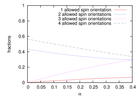
Figure 17: The relative frequency of the classes with $k=1$, $2$, $3$ or $4$ allowed spin orientations, at $\delta=\delta_{\rm c}=1.77521$, for variable angles of the Wolff direction and the two spins (with an allowed starting orientation).

The brute-force method is not a consistent cluster algorithm; this could be harmful for its efficiency. In view of its occasional accept/reject decision about cluster flips, and the additional heat bath step (which is required for the alteration of $|\alpha|$), this algorithm does not appear very promising. Hence we did not apply it, and it remains an interesting open question how to deal with the cases in the class $k=3$, and — more generally — how to construct a consistent cluster algorithm which involves a non-local variable, such as a dynamical boundary twist.

Appendix C Simulated annealing

For a given configuration, we first identify the $N$ vortices and $N$ anti-vortices. There are $N!$ possibilities to build vortex–anti-vortex pairs. For one option, they are separated by some Euclidean distances $d_{{\rm VA},\,i}$, $i=1\dots N$. For the considerations in Subsection 4.3 we search for the pairing which minimises the term $D^{2}$ in eq. (4.5). For comparison we also perform the optimal pairing among the vortices and among the anti-vortices. On the $L=128$ lattice, and $\delta$ close to — or above — $\delta_{\rm c}$, we cannot check all possibilities, since $N$ is of $O(100)$. Hence we resort to the technique of simulated annealing [43].

We start from one arbitrary pairing, measure $D^{2}$ and suggest a minimal modification by exchanging the partners among two pairs (which are randomly selected). Then we take a Metropolis-style decision about this modification: it is always accepted if $D^{2}_{\rm new}\leq D^{2}_{\rm old}$, and with probability $\exp([D^{2}_{\rm old}-D^{2}_{\rm new}]/T)$ otherwise. The parameter $T$ decreases as a monotonous annealing function of the number of $\tau$ of such annealing steps. We test 3 functions of this kind: linear, exponential and piecewise constant,

$$T(\tau)=\left\{\begin{array}[]{ccc}T_{0}(1-\tau/u)&&\tau/u<1\\ 0&&{\rm otherwise}\end{array}\right.\ ,\quad T(\tau)=T_{0}\cdot v^{1000\tau/u}\ ,$$ (C.1)

or the deformation of the linear decrease into stair steps. The constants are chosen as $T_{0}=100$, $u=10^{7}$ and $v=0.99$.

For a given configuration, we test $20$ initial pairings, all 3 annealing functions, and the process ends based on a “Cauchy criterion” (no change within 500 annealing steps). The lowest final $D^{2}$ value found in this way is in fact the global minimum for configurations with up to 14 vortices, as we checked by testing all pair formations. For higher vortex numbers we consider this way of searching for the global minimum still quite reliable, based on the consistency of the optimal solution identified in multiple runs, with distinct starting points and annealing functions.

References

- [1] J.M. Kosterlitz and D.J. Thouless, J. Phys. C 6 (1973) 1181.
- [2] M.R. Beasley, J.E. Mooij and T.P. Orlando, Phys. Rev. Lett. 42 (1979) 1165.
- [3] J. Fröhlich and T. Spencer, Commun. Math. Phys. 81 (1981) 527.
- [4] A.I. Belousov and Yu.E. Lozovik, Solid State Commun. 100 (1996) 421. C. Rojas and J.V. José, Phys. Rev. B 54 (1996) 12361.
- [5] A.N. Pargellis, S. Green and B. Yurke, Phys. Rev. E 49 (1994) 4250.
- [6] V.L. Berezinskii, Sov. Phys. JETP 32 (1970) 493; Sov. Phys. JETP 34 (1971) 610.
-
[7]
E.H. Lieb and F.Y. Wu, in “Phase Transitions
and Critical Phenomena”, edited by C. Domb and N.S. Green,
Academic Press (1972), vol. 1.
S.T. Chui and J.D. Weeks, Phys. Rev. B 14 (1976) 4978.
H. van Beijeren, Phys. Rev. Lett. 38 (1977) 993.
B. Nienhuis, Phys. Rev. Lett. 49 (1982) 1062. - [8] M. Hasenbusch and K. Pinn, J. Phys. A 30 (1997) 63.
- [9] R. Kenna and A.C. Irving, Nucl. Phys. B 485 (1997) 583.
- [10] R. Kenna, arXiv:cond-mat/0512356 [cond-mat.stat-mech].
- [11] J.M. Kosterlitz, J. Phys. C 7 (1974) 1046.
- [12] M. Hasenbusch, J. Phys. A 38 (2005) 5869.
- [13] J. Balog, M. Niedermaier, F. Niedermayer, A. Patrascioiu, E. Seiler and P. Weisz, Nucl. Phys. B 618 (2001) 315.
- [14] J. Balog, F. Knechtli, T. Korzec and U. Wolff, Nucl. Phys. B 675 (2003) 555.
- [15] W. Bietenholz, U. Gerber, M. Pepe and U.-J. Wiese, JHEP 1012 (2010) 020.
- [16] W. Bietenholz, M. Bögli, F. Niedermayer, M. Pepe, F.G. Rejón-Barrera and U.-J. Wiese, JHEP 1303 (2013) 141.
-
[17]
W. Bietenholz, A. Pochinsky and
U.-J. Wiese, Phys. Rev. Lett. 75 (1995) 4524.
M. Hasenbusch, Phys. Rev. D 53 (1996) 3445.
A. Patrascioiu and E. Seiler, J. Stat. Phys. 106 (2002) 811. - [18] M.E. Fisher, M.N. Barber and D. Jasnow, Phys. Rev. A 8 (1973) 1111.
- [19] P. Hasenfratz and H. Leutwyler, Nucl. Phys. B 343 (1990) 241.
-
[20]
D.R. Nelson and J.M. Kosterlitz,
Phys. Rev. Lett. 39 (1977) 1201.
P. Minnhagen and G.G. Warren, Phys. Rev. B 24 (1981) 2526. - [21] N.V. Prokof’ev and B.V. Svistunov, Phys. Rev. B 61 (2000) 11282.
-
[22]
T. Otha and D. Jasnow,
Phys. Rev. B 20 (1979) 139.
S. Teitel and C. Jayaprakash, Phys. Rev. B 27 (1983) 598. - [23] A. Pelissetto and E. Vicari, Phys. Rev. E 87 (2013) 032105.
- [24] P. Olsson and P. Holme, Phys. Rev. B 63 (2001) 052407.
- [25] H. Weber and P. Minnhagen, Phys. Rev. B 37 (1988) 5986.
- [26] P. Minnhagen and B.J. Kim, Phys. Rev. B 67 (2003) 172509.
- [27] J. Balog, J. Phys. A 34 (2001) 5237.
- [28] J. Balog, F. Niedermayer, M. Pepe, P. Weisz and U.-J. Wiese, JHEP 1211 (2012) 140.
- [29] U. Wolff, Phys. Rev. Lett. 62 (1989) 361.
- [30] M. Hasenbusch, J. Stat. Mech. (2008) P08003.
- [31] S. Miyashita, H. Nishimori, A. Kuroda and M. Suzuki, Prog. Theor. Phys. 60 (1978) 1669.
- [32] J. Tobochnik and G.V. Chester, Phys. Rev. B 20 (1979) 3761.
- [33] C. Bowen, D.L. Hunter and N. Jan, J. Stat. Phys. 69 (1992) 1097.
- [34] R. Gupta and C.F. Baillie, Phys. Rev. B 45 (1992) 2883.
- [35] H.-C. Chu and G.A. Williams, Phys. Rev. Lett. 86 (2001) 2585.
- [36] A. Jelić and L.F. Cugliandolo, J. Stat. Mech. (2011) P02032.
- [37] S.B. Ota and S. Ota, Phys. Lett. A 206 (1995) 133.
- [38] S. Aoki, H. Fukaya, S. Hashimoto and T. Onogi, Phys. Rev. D 76 (2007) 054508.
- [39] S. Aoki et al. (JLQCD and TWQCD Collaborations), Phys. Lett. B 665 (2008) 294.
- [40] W. Bietenholz, I. Hip, S. Shcheredin and J. Volkholz, Eur. Phys. J. C 72 (2012) 1938.
-
[41]
H. Fukaya, S. Hashimoto, T. Hirohashi,
K. Ogawa and T. Onogi,
Phys. Rev. D 73 (2006) 014503.
W. Bietenholz, K. Jansen, K.-I. Nagai, S. Necco, L. Scorzato and S. Shcheredin, JHEP 0603 (2006) 017. - [42] P. Olsson, Phys. Rev. B 52 (1995) 4511.
- [43] S. Kirkpatrick, C.D. Gelatt and M.P. Vecchi, Science 220 (1983) 671.