Two-colour QCD with heavy quarks at finite densities

Abstract

We extend the density-of-states approach to gauge systems (LLR method Langfeld et al. (2012)) to QCD at finite temperature and density with heavy quarks. The approach features an exponential error suppression and yields the Polyakov loop probability distribution function over a range of more than hundred orders of magnitude. SU(2) gauge theory is considered in the confinement and the high-temperature phase, and at finite densities of heavy quarks. In the latter case, a smooth rise of the density with the chemical potential is observed, and no critical phenomenon associated with deconfinement due to finite densities is found.

The phase structure of QCD is governed by two main phenomena, quark confinement and chiral symmetry breaking. At non-vanishing chemical potential this phase structure is unresolved yet despite the impressive progress made in the last two decades. On the one hand this relates to the sign-problem which hampers lattice computations at baryo-chemical potential $\mu_{B}/T\gtrsim 1$. On the other hand, first principle continuum methods at large chemical potential are hampered by the necessity of fully taking into account the hadronic resonance spectrum and the increasingly complicated ground state structure of QCD at finite density.

In QCD with static quarks, the confinement-deconfinement transition is a phase transition of first or second order, depending on the rank of the gauge group. The related order parameter is the expectation value of the Polyakov loop in the fundamental representation, $\langle P(\vec{x})\rangle$, Polyakov (1978); McLerran and Svetitsky (1981). It relates to the free energy of a single quark state. For $SU(N)$ the Polyakov loop is an order parameter for the order - disorder transition the centre of the gauge group. For $SU(2)$ the centre symmetry is $Z_{2}$, and the transition is of second order. It is conjectured that it belongs to the Ising universality class.

These findings have ever since stirred the hope that an effective theory of the Polyakov line might be based upon a rather simple action but still has a grasp of the confinement mechanism Pisarski (2000). In the last two decades, this idea has inspired numerous Polyakov loop enhanced quark-meson models. These models contain the Polyakov line as a remanent degree of freedom from the gluon sector, see e.g. Meisinger and Ogilvie (1996); Langfeld et al. (1997); Langfeld and Rho (1999); Fukushima (2004); Ratti et al. (2006); Megias et al. (2006); Schaefer et al. (2007) in terms of a Polyakov loop potential. More recently, it has been shown how these Polyakov loop enhanced low energy models of QCD are embedded in first principle QCD with the help of functional methods, Braun et al. (2010); Fister and Pawlowski (2013); Braun et al. (2011); Haas et al. (2013); Fischer et al. (2013). This entails that these model potentially give access to the phase structure of QCD and may offer explanations of heavy-ion-collision phenomena such as the excess in the dilepton production in collisions with heavy nuclei Langfeld et al. (1997).

Polyakov-loop enhanced models might also provide access to the QCD phase diagram at low temperatures and high baryon densities. Using an expansion with respect to inverse powers of the heavy quark mass, the QCD partition function can be systematically reduced to a theory of Polyakov lines, interacting with (spatial) gluons, for which the dependence on the baryon chemical potential is known Langfeld and Shin (2000). Integrating out the spatial gluon fields would leave us with the PLA at finite chemical potential which is, in fact, finite density QCD in the heavy quark limit. Many attempts have been made to guess this PLA by using symmetry arguments DeGrand and DeTar (1983) or by reducing the Polyakov line action to the simplest case of the nearest neighbour interactions Karsch and Wyld (1985). The latter so-called SU(3) spin model has served in the past as testbed for new simulations techniques which are designed to circumvent the notorious sign problem of dense matter systems Karsch and Wyld (1985); Aarts and James (2012); Mercado and Gattringer (2012). Another recent approach to the PLA at finite densities is the strong coupling approximation Langelage et al. (2011); Fromm et al. (2012). First studies show that scaling violations might be mild adding predictive power to this approach. A more systematic approach to PLA has been recently has been recently put forward: Using the relative-weights-method Greensite (2012), a surprisingly simple Polyakov line effective theory has been reported in momentum space at least in the confinement phase for the SU(2) gauge theory Greensite and Langfeld (2013).

The main obstacle for the calculation of the Polyakov line effective potential by means of Monte-Carlo simulations are cancellations that result in a poor signal-to-noise ratio. Recently a density-of-states method on the basis of the Wang-Landau approach Wang and Landau (2001) has been improved and made available for theories with continuous gauge groups Langfeld et al. (2012). The new method (called LLR method in the following) features an exponential error suppression and directly provides access to the partition function. It has been tested for the $U(1)$, $SU(2)$ and $SU(3)$ gauge theories with large volumes Langfeld et al. (2012).

In this letter, we generalise the LLR-method for the calculation of the Polyakov line effective potential with an unprecedented precision due to the exponential error suppression. We will use our numerical findings to study the properties of $SU(2)$ gauge theory at finite densities of heavy quarks.

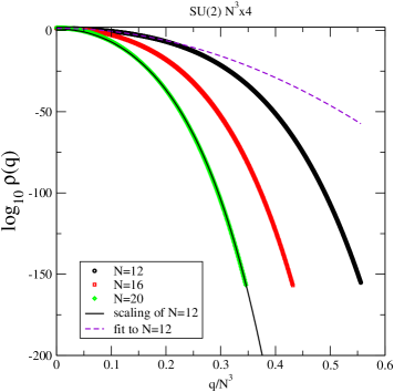
Figure 1: The Polyakov line probability distribution $\rho(q)$ (9) for a lattice size of $N^{3}\times 4$, $N=12,\,16,\,20$ in the confinement phase ($\beta=2.2$).

Our simulations are based upon the Wilson action using a $N\times N_{t}$ lattice. The gluonic degrees of freedom are represented by unitary matrices $U_{\mu}(x)$ associated with the links of the lattice. The Polyakov line $P(\vec{x})$ is the ordered product of the time-like links,

$$P(\vec{x})\;=\;\frac{1}{2}\,\hbox{tr}\,\prod_{t}\,U_{0}(\vec{x},t)\;.$$ (1)

The effective potential $V$ is derived by a Legendre transformation from the generating functional $Z[j]$,

$$Z[j] = \int{\cal D}U_{\mu}\;\exp\left\{S_{g}[U]+j\,\sum_{\vec{x}}P(\vec{x})\right\},$$ (2)

with

$$V(q) = \frac{T}{\Omega_{3}}\,\Bigl{(}j\,q-\ln Z[j]\Bigr{)}\;,\qquad q=\frac{d\,\ln Z[j]}{dj}\;.$$ (3)

Here $S_{g}$ is the Wilson action, and $\Omega_{3}$ is the spatial volume. We also consider a non-vanishing chemical potential $\mu$ which couples to heavy and static quarks. In the heavy quark limit the quark determinant can be explicitly calculated Langfeld and Shin (2000). The complete action can be approximated by

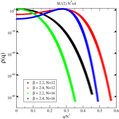
Figure 2: The Polyakov line probability distribution $\rho(q)$ (9) for a lattice size of $N^{3}\times 4$, $N=12,\,16$ in the confinement phase ($\beta=2.2$) and in the deconfined phase ($\beta=2.4$).

$$S[U] = S_{g}[U]\;+\;f\,\sum_{\vec{x}}P(\vec{x})\;,$$ (4)

with the ‘relative fugacity’ $f$,

$$f = \frac{\sqrt{2}}{\pi^{3/2}}(mT)^{3/2}\,a^{3}\,\exp\left\{\frac{\mu-m}{T}\right\}\;.$$ (5)

Here, $m$ is the heavy quark mass, $T$ the temperature and $a$ the lattice spacing. Note that the derivation of the result (4) neglects terms with multiple windings of the Polyakov line around the torus. This approximation is only justified for chemical potentials smaller than or close to the mass gap Langfeld and Shin (2000). As a result, we do not observe the saturation of the baryonic density for $\mu\gg m$ which takes place on finite lattices when the lattice is filled with quarks. Here, we consider (4) as a ”weak coupling” extension of the popular Polyakov loop model Mercado et al. (2011); Gattringer (2011) and take it for granted for the remainder of the paper. With this assumption, $f$ merely shifts the external source $j$ in (2), and we find

$$V(q;f)\;=\;V(q)\;+\;T\,f\,q/\Omega_{3}\;.$$ (6)

It is generically difficult to calculate the effective potential $V(q)$ defined in (3) by means of Monte-Carlo simulations. The reason for this is that the Polyakov line $q$ in (3) is an extensive observable, which scales with the spatial volume:

$$q\;=\;N^{3}\,\langle P(\vec{x})\rangle(j)\;.$$

Hence, the term $\exp\{jq\}$ in the partition function is generically large, i.e., of order $N^{3}$, but is cancelled to a good deal by the “classical term” in (3), i.e., $-jq$, leaving us with a poor signal-to-noise ratio.

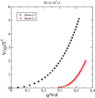
Figure 3: The Polyakov line effective potential $V(q)$ (3) for a lattice size of $16^{3}\times 4$ for $\beta=2.2$ and $\beta=2.4$.

In the present work we adopt the improved Wang-Landau approach presented in Langfeld et al. (2012) for the calculation of the partition function $Z[j]$ to a very high precision. Central to this approach is the generalised density of states for the Polyakov line,

$$\rho(q)\;=\;\int{\cal D}U_{\mu}\;\mathrm{e}^{S_{g}[U]}\;\delta\Bigl{(}q-p[U]\Bigr{)}\;,$$ (7)

where

$$p[U]\;=\;\sum_{\vec{x}}P(x)\;,$$

with $P(x)$ defined in (1). If we manage to obtain a high precision result for $\rho(q)$, the partition function is recovered by standard integration,

$$Z[j]\;=\;\int dq\;\rho(q)\;\exp\{j\,q\}\;.$$ (8)

To obtain the density-of-states $\rho$ numerically, we approximate its logarithm by a piecewise linear function,

$$\rho(q)\;=\;\rho(q_{0})\,\exp\Bigl{\{}a(q_{0})\,(q-q_{0})\Bigr{\}}\,,$$ (9)

for $q_{0}\leq q<q_{0}+\delta q$. We generalise the LLR approach and define the truncated and re-weighted expectation values of present case by

$${\langle\kern-1.69998pt\langle}f(q){\rangle\kern-1.69998pt\rangle}(a)=\frac{1}{\cal N}\int_{[q_{0},\delta q]}\hskip-14.22636pt{\cal D}U_{\mu}\,\mathrm{e}^{S_{g}[U]}\,f\Bigl{(}p[U]\Bigr{)}\;\mathrm{e}^{-ap[U]},$$ (10)

with

$${\cal N} = \int_{[q_{0},\delta q]}{\cal D}U_{\mu}\;\mathrm{e}^{S_{g}[U]}\;\mathrm{e}^{-ap[U]}\;.$$ (11)

These expectation values can be calculated by straightforward Monte-Carlo simulations. Thereby, the integration only extends over configurations $\{U\}$ with $q_{0}<p([U])<q_{0}+\delta q$. In practice, this constraint is implemented as follows: we start with an ‘empty vacuum’ configuration where all links are set to the unit element. We then set the time-like links at the time slice $t=1$ according to,

$$U_{0}(1,\vec{x})=\cos\theta+i\sin\theta\tau^{3},$$ (12)

with

$$\cos\theta=\left(q_{0}+\frac{\delta q}{2}\right)/N^{3}.$$ (13)

This generates an ‘allowed’ configuration with $p[U]$ inside the desired interval. Subsequent Markov chain updates make sure that an update is disregarded (probability zero) if the configurations $p[U]$ would fall outside the interval. We then follow the standard procedures: after thermalisation, we perform“dummy” sweeps between measurements. For the determination of $a(q_{0})$, we follow the technique detailed in Langfeld et al. (2012). This technique exploits the fact that we find

$${\langle\kern-1.69998pt\langle}\Delta q{\rangle\kern-1.69998pt\rangle}(a)=0,\hbox to28.45274pt{\hfill}\delta q=q-\left(q_{0}+\frac{\delta q}{2}\right)\,,$$

if the re-weighting factor $\exp\{-ap[U]\}$ compensates the true density-of-states. This is a non-linear equation which we solve for $a$ using the iteration:

$$a_{n+1}\;=\;a_{n}\,+\,\lambda\,\frac{12}{\delta q^{2}}{\langle\kern-1.69998pt\langle}\Delta q{\rangle\kern-1.69998pt\rangle}(a_{n}).$$

Thereby, $\lambda<1$ is an under-relaxation factor which we found useful to control the amount of noise in during the iteration. The precise value of $\lambda$ is not critical, and we worked with $\lambda=0.25$ most of the time. We repeat these steps for any $q_{0}$ out of the range of interest and reconstruct the density-of-states $\rho(q)$ (9), i.e., the Polyakov line probability distribution.

We have studied the Polyakov line distribution function $\rho(q)$ (9) for several lattice sizes $N^{3}\times 4$ for $\beta=2.2$ and for $\beta=2.4$. For this temporal extent, the deconfinement phase transition occurs for $\beta\approx 2.3$ which leaves us with $\beta=2.2$ in the confinement phase and for $\beta=2.4$ well in the high temperature deconfined phase. Let us firstly consider the confinement phase. In order to check our new numerical method, we have also calculated $\rho(q)$ by histogramming the Polyakov line obtained by a standard heat-bath simulation. In the small $q$ range, $q<0.05$, where a reasonable of amount of statistics can be obtained by the standard method, we find a good agreement. We stress that our new method can easily produce results for $q$ as large as $0.4$ and provides access to the probability distribution over more than hundred orders of magnitude with good precision. The (logarithms base $10$ of the) probability distributions $\rho(q)$ are shown in Figure 1 for several spatial values. The error bars have been obtained with the bootstrap method and are well with the plotting symbols. As expected, the probability distributions centre around the trivial value $q=0$. The distributions get narrower with increasing spatial volume. In fact, one expects that $\mathrm{log}_{10}\rho(q)$ scales with number of degrees of freedom and therefore with the volume $\Omega_{3}$. To put this to the test, we have rescaled the $N=12$ results to match with the $N=20$ distribution. After a proper normalisation of the distribution, the result is shown in Figure 1, solid line. We find an almost perfect match. We also point out that the distribution $\rho(q)$ of the Polyakov line is far from Gaussian. To this aim, we have fitted the low $q$ range of $\mathrm{log}_{10}\rho(q)$ at $N=12$ to a parabola. The result of this fit (dashed line in Figure 1) shows large deviations from the quadratic behaviour even at moderate values of $q$.

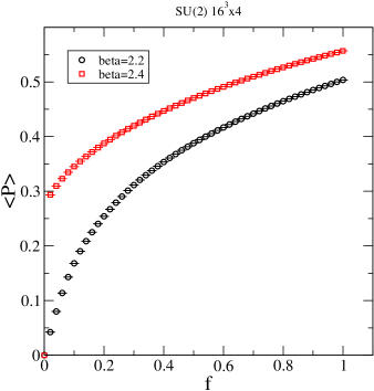
Figure 4: The Polyakov line expectation value $P$ for a $16^{3}\times 4$ lattice, $\beta=2.2$ and $\beta=2.4$.

The probability distributions of the confined and the high-temperature phase are compared in Figure 2. In the latter phase ($\beta=2.4$), the most likely value for $q$ is different from zero indicating the spontaneous breakdown of the centre symmetry. Again the distribution functions get narrower with increasing spatial volume leaving us with a decreasing value for $\rho$ at $q=0$. One expects that $\rho(q=0)$ vanishes in the infinite volume limit realising the spontaneous symmetry breakdown. A more systematic volume study of this effect will be presented elsewhere.

It turns out that the precision of the data is good enough to attempt the Legendre transformation and to directly obtain the Polyakov line effective potential. To this aim, we choose $j$ as an implicit parameter and obtain the partition function by means of (8) and $q$ by

$$q(j)\;=\;\frac{\int dq^{\prime}\;\rho(q^{\prime})\;q^{\prime}\;\exp\{j\,q^{\prime}\}}{\int dq^{\prime}\;\rho(q^{\prime})\;\exp\{j\,q^{\prime}\}}.$$

Substituting both into (3) allows us to obtain the potential in implicit form. Error bars are obtained by the bootstrap method. The related result is shown in Figure 3. In both cases, i.e., $\beta=2.2$ and $\beta=2.4$, the potential is convex. For the deconfinement case, the potential is flat until $q\approx 0.3$ indicating the spontaneous breakdown of centre symmetry. The absolute values of the potential in units of the temperature are quite high when compared to the results from ab initio continuum methods. We stress that only the unrenormalised potential as function of the unrenormalised Polyakov line is shown in Figure 3. To prepare the grounds for a comparison, simulations with more values of $\beta$ and several lattice sizes are need to renormalise and extrapolate to the continuum limit. This is left to future work.

Now we apply our approach to two-colour QCD at finite densities of heavy quarks. The baryon number $B$ can be retrieved from the partition function by

$$B\;=\;T\,\frac{d\ln Z}{d\mu}\;=\;f\,\langle p[U]\rangle\;,$$ (14)

where we have used (4) and (5). We will use the heavy quark mass $m$ as the fundamental scale to present our results: We define the baryon density (in units of $m$) as

$$\rho_{B}/m^{3} := B/(Vm^{3})$$ (15)

$$= \sqrt{2}\,\left(\frac{T}{m\pi}\right)^{3/2}\mathrm{e}^{(\mu-m)/T}\;\frac{1}{N^{3}}\langle p[U]\rangle\;.$$

In the heavy quark limit (and within the remit of the approximations leading to (4), $\rho_{B}$ is proportional the Polyakov line expectation value. Our high precision results for $\langle P\rangle=\langle p[U]\rangle/N^{3}$ are shown in Figure 4 for the phases below and above the deconfinement transition. While $\langle P\rangle$ goes to zero for vanishing fugacity $f$ in the confinement phase, $\langle P\rangle$ remains finite in the same limit for the high temperature phase. The reason for this is that any small non-vanishing value for $f$ triggers a sizeable response for $\langle P\rangle$ because of the spontaneously broken centre symmetry in the high temperature phase.

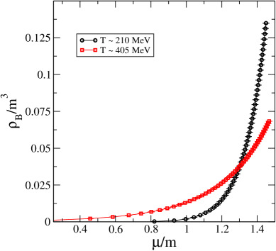
Figure 5: The baryon density $\rho_{B}$ for ”charmonium” as a function of the chemical potential $\mu$ in units of the charmonium mass $m$ in the confinement phase $(T\approx 210\mathrm{MeV})$ and in the gluon plasma phase $(T\approx 405\mathrm{MeV})$.

Let us now investigate the response of the baryon density to the chemical potential for the two-colour analogue of charmonium with $m=1.29\,$GeV. For vanishing temperature, the fugacity $f$ vanishes as well for chemical potentials smaller than the mass gap, i.e., $\mu<m$. Thus, the onset value coincides with the mass $m$, and a Silver Blaze problem Cohen (2003) is absent in our approach. In the following, we consider two temperatures well above and well below the confinement-deconfinement temperature. The temperature is generically given by

$$T\;=\;\frac{1}{N_{t}a}\;=\;\frac{\sqrt{\sigma}}{N_{t}\sqrt{\sigma a^{2}}}\;,$$

where the lattice spacing is measured in units of the string tension. We use $\sigma a^{2}(\beta=2.2)=0.28(1)$ and $\sigma a^{2}(\beta=2.4)=0.0738(5)$, see e.g. Langfeld and Shin (2000). With the standard value $\sigma=(440\mathrm{MeV})^{2}$ and for a $16^{3}\times 4$, $N_{t}=4$ lattice, we are left with temperatures $T(\beta=2.2)=210\,$MeV, well below transition temperature $T_{c}\approx 300\,$ MeV, and $T(\beta=2.4)=405\,$MeV in the deconfinement phase. Our findings are summarised in Figure 5: In the confinement phase and for chemical potentials below the onset value, the response of the density to $\mu$ is much weaker than in the gluon plasma phase. The physics behind this observation is that in the confinement phase temperature effects need to excite a baryon whereas in the plasma phase single quark excitations are allowed.

Let us now discuss the existence of a density driven phase transition in heavy quark SU(2) Yang-Mills theory. Within the remit of the approximations leading to the effective theory (4), we do not expect that a phase transition exists: Since the fugacity $f$ directly couples to the Polyakov line, any small value implies that Polyakov line potential flattens at large distances $|\vec{x}|$,

$$\langle P(\vec{x})P(0)\rangle\to\langle P\rangle^{2}(f)\not=0\,.$$ (16)

This property relates to the breaking of the colour electric flux tube: the colour electric flux tube, which connects a quark and a anti-quark test charge, can break and attach to one of the static background charges. Hence, deconfinement sets in at the onset value $\mu=m$. The situation is similar to the $O(2)$ quantum model for which superfluidity occurs at the critical chemical potential Langfeld (2013). We point out that lattice simulations and effective model computations of dense two-colour QCD found a more rich state of matter for chemical potentials close to the onset value, for recent results see e.g. Cotter et al. (2013); Boz et al. (2013); Strodthoff and von Smekal (2013). This is (i) due to the finite quark masses in Q₂D and (ii) due to the neglect of higher Polyakov windings in the built-up to (4). These contributions are potentially important to describe physics such as the transition from BEC to BCS.

Acknowledgments: We thank Antonio Rago for helpful discussions. This work is supported by STFC under the DiRAC framework, by the Helmholtz Alliance HA216/EMMI and by ERC- AdG-290623. We are grateful for the support from the HPCC Plymouth, where the numerical computations have been carried out.

References

- Langfeld et al. (2012) K. Langfeld, B. Lucini, and A. Rago, Phys.Rev.Lett. 109, 111601 (2012), eprint 1204.3243.
- Polyakov (1978) A. M. Polyakov, Phys.Lett. B72, 477 (1978).
- McLerran and Svetitsky (1981) L. D. McLerran and B. Svetitsky, Phys.Rev. D24, 450 (1981).
- Pisarski (2000) R. D. Pisarski, Phys.Rev. D62, 111501 (2000), eprint hep-ph/0006205.
- Meisinger and Ogilvie (1996) P. N. Meisinger and M. C. Ogilvie, Phys.Lett. B379, 163 (1996), eprint hep-lat/9512011.
- Langfeld et al. (1997) K. Langfeld, H. Reinhardt, and M. Rho, Nucl.Phys. A622, 620 (1997), eprint hep-ph/9703342.
- Langfeld and Rho (1999) K. Langfeld and M. Rho, Nucl.Phys. A660, 475 (1999), eprint hep-ph/9811227.
- Fukushima (2004) K. Fukushima, Phys.Lett. B591, 277 (2004), eprint hep-ph/0310121.
- Ratti et al. (2006) C. Ratti, M. A. Thaler, and W. Weise, Phys.Rev. D73, 014019 (2006), eprint hep-ph/0506234.
- Megias et al. (2006) E. Megias, E. Ruiz Arriola, and L. Salcedo, Phys.Rev. D74, 065005 (2006), eprint hep-ph/0412308.
- Schaefer et al. (2007) B.-J. Schaefer, J. M. Pawlowski, and J. Wambach, Phys.Rev. D76, 074023 (2007), eprint 0704.3234.
- Braun et al. (2010) J. Braun, H. Gies, and J. M. Pawlowski, Phys.Lett. B684, 262 (2010), eprint 0708.2413.
- Fister and Pawlowski (2013) L. Fister and J. M. Pawlowski (2013), eprint 1301.4163.
- Braun et al. (2011) J. Braun, L. M. Haas, F. Marhauser, and J. M. Pawlowski, Phys.Rev.Lett. 106, 022002 (2011), eprint 0908.0008.
- Haas et al. (2013) L. M. Haas, R. Stiele, J. Braun, J. M. Pawlowski, and J. Schaffner-Bielich (2013), eprint 1302.1993.
- Fischer et al. (2013) C. S. Fischer, L. Fister, J. Luecker, and J. M. Pawlowski (2013), eprint 1306.6022.
- Langfeld and Shin (2000) K. Langfeld and G. Shin, Nucl.Phys. B572, 266 (2000), eprint hep-lat/9907006.
- DeGrand and DeTar (1983) T. A. DeGrand and C. E. DeTar, Nucl.Phys. B225, 590 (1983).
- Karsch and Wyld (1985) F. Karsch and H. Wyld, Phys.Rev.Lett. 55, 2242 (1985).
- Aarts and James (2012) G. Aarts and F. A. James, JHEP 1201, 118 (2012), eprint 1112.4655.
- Mercado and Gattringer (2012) Y. D. Mercado and C. Gattringer, Nucl.Phys. B862, 737 (2012), eprint 1204.6074.
- Langelage et al. (2011) J. Langelage, S. Lottini, and O. Philipsen, JHEP 1102, 057 (2011), eprint 1010.0951.
- Fromm et al. (2012) M. Fromm, J. Langelage, S. Lottini, and O. Philipsen, JHEP 1201, 042 (2012), eprint 1111.4953.
- Greensite (2012) J. Greensite, Phys.Rev. D86, 114507 (2012), eprint 1209.5697.
- Greensite and Langfeld (2013) J. Greensite and K. Langfeld (2013), eprint 1301.4977.
- Wang and Landau (2001) F. Wang and D. P. Landau, Phys. Rev. Lett. 86, 2050 (2001).
- Mercado et al. (2011) Y. D. Mercado, H. G. Evertz, and C. Gattringer, Phys.Rev.Lett. 106, 222001 (2011), eprint 1102.3096.
- Gattringer (2011) C. Gattringer, Nucl.Phys. B850, 242 (2011), eprint 1104.2503.
- Cohen (2003) T. D. Cohen, Phys.Rev.Lett. 91, 222001 (2003), eprint hep-ph/0307089.
- Langfeld (2013) K. Langfeld, Phys. Rev. D 87, 114504 (2013), eprint 1302.1908.
- Cotter et al. (2013) S. Cotter, P. Giudice, S. Hands, and J.-I. Skullerud, Phys.Rev. D87, 034507 (2013), eprint 1210.4496.
- Boz et al. (2013) T. Boz, S. Cotter, L. Fister, D. Mehta, and J.-I. Skullerud (2013), eprint 1303.3223.
- Strodthoff and von Smekal (2013) N. Strodthoff and L. von Smekal (2013), eprint 1306.2897.