Transmission spectrum of Earth as a transiting exoplanet
from the ultraviolet to the near-infrared

Abstract

Transmission spectroscopy of exoplanets is a tool to characterize rocky planets and explore their habitability. Using the Earth itself as a proxy, we model the atmospheric cross section as a function of wavelength, and show the effect of each atmospheric species, Rayleigh scattering and refraction from 115 to 1000 nm. Clouds do not significantly affect this picture because refraction prevents the lowest 12.75 km of the atmosphere, in a transiting geometry for an Earth-Sun analog, to be sampled by a distant observer. We calculate the effective planetary radius for the primary eclipse spectrum of an Earth-like exoplanet around a Sun-like star. Below 200 nm, ultraviolet (UV) O₂ absorption increases the effective planetary radius by about 180 km, versus 27 km at 760.3 nm, and 14 km in the near-infrared (NIR) due predominantly to refraction. This translates into a 2.6% change in effective planetary radius over the UV-NIR wavelength range, showing that the ultraviolet is an interesting wavelength range for future space missions.

1. Introduction

Many planets smaller than Earth have now been detected with the Kepler mission, and with the realization that small planets are much more numerous than giant ones (Batalha et al. 2013), future space missions, such as the James Webb Space Telescope (JWST), are being planned to characterize the atmosphere of potential Earth analogs by transiting spectroscopy, explore their habitability, and search for signs of life. The simultaneous detection of large abundances of either O₂ or O₃ in conjunction with a reducing species such as CH₄, or N₂O, are biosignatures on Earth (see e.g. Des Marais et al. 2002; Kaltenegger et al. 2010a and reference therein). Although not a clear indicative for the presence of life, H₂O is essential for life.

Simulations of the Earth’s spectrum as a transiting exoplanet (Ehrenreich et al. 2006; Kaltenegger & Traub 2009; Pallé et al. 2009; Vidal-Madjar et al. 2010; Rauer et al. 2011; García Muñoz et al. 2012; Hedelt et al. 2013) have focused primarily on the visible (VIS) to the infrared (IR), the wavelength range of JWST (600-5000 nm). No models of spectroscopic signatures of a transiting Earth have yet been computed from the mid- (MUV) to the far-ultraviolet (FUV). Which molecular signatures dominate this spectral range? In this paper, we present a model of a transiting Earth’s transmission spectrum from 115 to 1000 nm (UV-NIR) during primary eclipse. While no UV missions are currently in preparation, this model can serve as a basis for future UV mission concept studies.

2. Model description

To simulate the spectroscopic signatures of an Earth-analog transiting its star, we modified the Smithsonian Astrophysical Observatory 1998 (SAO98) radiative transfer code (see Traub & Stier 1976; Johnson et al. 1995; Traub & Jucks 2002; Kaltenegger & Traub 2009 and references therein for details), which computes the atmospheric transmission of stellar radiation at high spectral resolution from a molecular line list database. Updates include a new database of continuous absorber’s cross sections, as well as N₂, O₂, Ar, and CO₂ Rayleigh scattering cross sections from the ultraviolet (UV) to the near-infrared (NIR). A new module interpolates these cross sections and derives resulting optical depths according to the mole fraction of the continuous absorbers and the Rayleigh scatterers in each atmospheric layer. We also compute the deflection of rays by atmospheric refraction to exclude atmospheric regions for which no rays from the star can reach the observer due to the observing geometry.

Our database of continuous absorbers is based on the MPI-Mainz-UV-VIS Spectral Atlas of Gaseous Molecules. For each molecular species of interest (O₂, O₃, CO₂, CO, CH₄, H₂O, NO₂, N₂O, and SO₂), we created model cross sections composed of several measured cross sections from different spectral regions, at different temperatures when measurements are available, with priority given to higher spectral resolution measurements (see Table 1). We compute absorption optical depths for different altitudes in the atmosphere using the cross section model with the closest temperature to that of the atmospheric layer considered. Note that we do not consider line absorption from atomic or ionic species which could produce very narrow but possibly detectable features at high spectral resolution (see also Snellen et al. 2013).

The Rayleigh cross sections, $\sigma_{R}$, of N₂, O₂, Ar, and CO₂, which make-up 99.999% of the Earth’s atmosphere, are computed with

$${\sigma_{R}}=\frac{32\pi^{3}}{3}\left(\frac{{\nu_{0}}}{n_{0}}\right)^{2}w^{4}F_{K},$$ (1)

where $\nu_{0}$ is the refractivity at standard pressure and temperature (or standard refractivity) of the molecular species, $w$ is the wavenumber, $F_{K}$ is the King correction factor, and $n_{0}$ is Loschmidt’s constant. Various parametrized functions are used to describe the spectral dependence of $\nu_{0}$ and $F_{K}$. Table 2 gives references for the functional form of both parameters, as well as their spectral region.

The transmission of each atmospheric layer is computed with Beer’s law from all optical depths. We use disc-averaged quantities for our model atmosphere.

We use a present-day Earth vertical composition (Kaltenegger et al. (2010b) for SO₂; Lodders & Fegley, Jr. (1998) for Ar; and Cox (2000) for all other molecules) up to 130 km altitude, unless specified otherwise. Above 130 km, we assume constant mole fraction with height for all the molecules except for SO₂ which we fix at zero, and for N₂, O₂, and Ar which are described below. Below 100 km, we use the US 1976 atmosphere (COESA 1976) as the temperature-pressure profile. Above 100 km, the atmospheric density is sensitive to and increases with solar activity (Hedin 1987). We use the tabulated results of the MSIS-86 model, for solar maximum (Table A1.2) and solar minimum conditions (Table A1.1) published in Rees (1989), to derive the atmospheric density, pressure, and mole fractions for N₂, O₂, and Ar above 100 km. We run our simulations in two different spectral regimes. In the VIS-NIR, from 10000 to 25000 cm^-1 (400-1000 nm), we use a 0.05 cm^-1 grid, while in the UV from 25000 to 90000 cm^-1 (111-400 nm), we use a 0.5 cm^-1 grid. For displaying the results, the VIS-NIR and the UV simulations are binned on a 4 cm^-1 and a 20 cm^-1 grid, respectively. The choice in spectral resolution impacts predominantly the detectability of spectral features.

The column abundance of each species along a given ray is computed taking into account refraction, tracing specified rays from the observer back to their source. Each ray intersects the top of the model atmosphere with an impact parameter $b$, the projected radial distance of the ray to the center of the planetary disc as viewed by the observer. As rays travel through the planetary atmosphere, they are bent by refraction along paths define by an invariant $L=(1+\nu(r))r\sin\theta(r)$ where both the zenith angle, $\theta(r)$, of the ray, and the refractivity, $\nu(r)$, are functions of the radial position of the ray with respect to the center of the planet. The refractivity is given by

$$\nu(r)=\left(\frac{n(r)}{n_{0}}\right)\sum_{j}f_{j}(r){\nu_{0}}_{j}=\left(\frac{n(r)}{n_{0}}\right)\nu_{0}(r),$$ (2)

where ${\nu_{0}}_{j}$ is the standard refractivity of the j^th molecular species while $\nu_{0}(r)$ is that of the atmosphere, $n(r)$ is the local number density, and $f_{j}(r)$ is the mole fraction of the j^th species. Here, we only consider the main contributor to the refractivity (N₂, O₂, Ar, and CO₂) which are well-mixed in the Earth’s atmosphere, and fix the standard refractivity at all altitudes at its surface value.

If we assume a zero refractivity at the top of the atmosphere, the minimum radial position from the planet’s center, $r_{min}$, that can be reached by a ray is related to its impact parameter by

$$L=(1+\nu(r_{min}))r_{min}=R_{top}\sin\theta_{0}=b,$$ (3)

where $R_{top}$ is the radial position of the top of the atmosphere and $\theta_{0}$ is the zenith angle of the ray at the top of the atmosphere. Note that $b$ is always larger than $r_{min}$, therefore the planet appears slightly larger to a distant observer. For each ray, we specify $r_{min}$, compute $\nu(r_{min})$, and obtain the corresponding impact parameter. Then, each ray is traced through the atmosphere every 0.1 km altitude increment, and column abundances, average mole fractions, as well as cumulative deflection along the ray are computed for each atmospheric layer (Johnson et al. 1995; Kaltenegger & Traub 2009).

We characterize the transmission spectrum of the exoplanet using effective atmospheric thickness, $\Delta z_{eff}$, the increase in planetary radius due to atmospheric absorption during primary eclipse. To compute $\Delta z_{eff}$ for an exoplanet, we first specify $r_{min}$ for $N$ rays spaced in constant altitude increments over the atmospheric region of interest. We then compute the transmission, $T$, and impact parameter, $b$, of each ray through the atmosphere, and finally use,

$$R_{eff}^{2}=R_{top}^{2}-\sum_{i=1}^{N}\left(\frac{T_{i+1}+T_{i}}{2}\right)(b_{i+1}^{2}-b_{i}^{2})$$ (4a)

$$R_{top}=R_{p}+\Delta z_{atm}$$ (4b)

$$\Delta z_{eff}=R_{eff}-R_{p},$$ (4c)

where $R_{eff}$ is the effective radius of the planet, $R_{top}$ is the radial position of the top of the atmosphere, $R_{p}$ is the planetary radius (6371 km), $\Delta z_{atm}$ is the thickness of the atmosphere, and $i$ denotes the ray considered. Note that $(N+1)$ refer to a ray that grazes the top of the atmosphere. The rays define $N$ projected annuli whose transmission is the average of the values at the borders of the annulus. The top of the atmosphere is defined where the transmission is 1, and no bending occurs ($b_{N+1}=R_{top}$). We choose R_top where atmospheric absorption and refraction are negligible, and use 100 km in the VIS-NIR, and 200 km in the UV for $\Delta z_{atm}$.

To first order, the total deflection of a ray through an atmosphere is proportional to the refractivity of the deepest atmospheric layer reached by a ray (Goldsmith 1963). The planetary atmosphere density increases exponentially with depth, therefore some of the deeper atmospheric regions can bend all rays away from the observer (see e.g. Sidis & Sari 2010, García Muñoz et al. 2012), and will not be sampled by the observations. At which altitudes this occurs depends on the angular extent of the star with respect to the planet. For an Earth-Sun analog, rays that reach a distant observer are deflected on average no more than 0.269$\arcdeg$. We calculate that the lowest altitude reached by these grazing rays range from about 14.62 km at 115 nm, 13.86 km at 198 nm (shortest wavelength for which all used molecular standard refractivities are measured), to 12.95 km at 400 nm, and 12.75 km at 1000 nm.

As this altitude is relatively constant in the VIS-NIR, we incorporate this effect in our model by excluding atmospheric layers below 12.75 km. To determine the effective planetary radius, we choose standard refractivities representative of the lowest opacities within each spectral region: 2.88$\times 10^{-4}$ for the VIS-NIR, and 3.00$\times 10^{-4}$ for the UV. We use 80 rays from 12.75 to 100 km in the VIS-NIR, and 80 rays from 12.75 to 200 km altitude in the UV. In the UV, the lowest atmospheric layers have a negligible transmission, thus the exact exclusion value of the lowest atmospheric layer, calculated to be between 14.62 and 12.75 km, do not impact the modeled UV spectrum.

3. Results and discussion

The increase in planetary radius due to the additional atmospheric absorption of a transiting Earth-analog is shown in Fig. 1 from 115 to 1000 nm.

The individual contribution of Rayleigh scattering by N₂, O₂, Ar, and CO₂ is also shown, with and without the effect of refraction by these same species, respectively. The individual contribution of each species, shown both in the lower panel of Fig. 1 and in Fig. 2, are computed by sampling all atmospheric layers down to the surface, assuming the species considered is the only one with a non-zero opacity. In the absence of absorption, the effective atmospheric thickness is about 1.8 km, rather than zero, because the bending of the rays due to refraction makes the planet appear larger to a distant observer.

The spectral region shortward of 200 nm is shaped by O₂ absorption and depends on solar activity. Amongst the strongest O₂ features are two narrow peaks around 120.5, and 124.4 nm, which, increase the planetary radius by 179-185 and 191-195 km, respectively. The strongest O₂ feature, the broad Schumann-Runge continuum, increases the planetary radius by more than 150 km from 134.4 to 165.5 nm, and peaks around 177-183 km. The Schumann-Runge bands, from 180 to 200 nm, create maximum variations of 30 km in the effective planetary radius. O₂ features can also be seen in the VIS-NIR, but these are much smaller than in the UV. Two narrows peaks around 687.0 and 760.3 nm increase the planetary radius to about 27 km, at the spectral resolution of the simulation.

Ozone absorbs in two different broad spectral regions in the UV-NIR increasing the planetary radius by 66 km around 255 nm (Hartley band), and 31 km around 602 nm (Chappuis band). Narrow ozone absorption, from 310 to 360 nm (Huggins band), produce variations in the effective planetary radius no larger than 2.5 km. Weak ozone bands are also present throughout the VIS-NIR: all features not specifically identified on the small VIS-NIR panel in Fig. 1 are O₃ features, and show changes in the effective planetary radius on the order of 1 km.

NO₂ and H₂O are the only other molecular absorbers that create observable features in the spectrum (Fig. 1, small VIS-NIR panel). NO₂ shows a very weak band system in the visible shortward of 510 nm, which produces less than 1 km variations in the effective planetary radius. H₂O features are observable only around 940 nm, where they increase the effective planetary radius to about 14.5 km.

Rayleigh scattering (Fig. 1) increases the planetary radius by about 68 km at 115 nm, 27 km at 400 nm, and 5.5 km at 1000 nm, and dominates the spectrum from about 360 to 510 nm where few molecules in the Earth’s atmosphere absorb, and refraction is not yet the dominant effect. In this spectral region, NO₂ is the dominant molecular absorber but its absorption is much weaker than Rayleigh scattering.

The lowest 12.75 km of the atmosphere is not accessible to a distant observer because no rays below that altitude can reach the observer in a transiting geometry for an Earth-Sun analog. Clouds located below that altitude do not influence the spectrum and can therefore be ignored in this geometry. Figure 1 also shows that refraction influences the observable spectrum for wavelengths larger than 400 nm.

The combined effects of refraction and Rayleigh scattering increases the planetary radius by about 27 km at 400 nm, 16 km at 700 nm, and 14 km at 1000 nm. In the UV, the lowest 12.75 km of the atmosphere have negligible transmission, so this atmospheric region can not be seen by a distant observer irrespective of refraction.

Both Rayleigh scattering and refraction can mask some of the signatures from molecular species. For instance, the individual contribution of the H₂O band in the 900-1000 nm region can increase the planetary radius by about 10 km. However, H₂O is concentrated in the lowest 10-15 km of the Earth’s atmosphere, the troposphere, hence its amount above 12.75 km increases the planetary radius above the refraction threshold only by about 1 km around 940 nm. The continuum around the visible O₂ features is due to the combined effects of Rayleigh scattering, ozone absorption, and refraction. It increases the effective planetary radius by about 21 and 17 km around 687.0 and 760.3 nm, respectively. The visible O₂ features add 6 and 10 km to the continuum values, at the spectral resolution of the simulation.

Figure 3 compares our effective model from Fig. 1 with atmospheric thickness with the one deduced by Vidal-Madjar et al. (2010) from Lunar eclipse data obtained in the penumbra. The contrast of the two O₂ features are comparable with those in the data. However, there is a slight offset (about 3.5 km) and a tilt in the main O₃ absorption profile. Note that, Vidal-Madjar et al. (2010) estimate that several sources of systematic errors and statistical uncertainties prevent them from obtaining absolute values better than $\pm$2.5 km. Also, we do not include limb darkening in our calculations. However, for a transiting Earth, the atmosphere eclipses an annular region on the Sun, whereas during Lunar eclipse observations, it eclipses a band across the Sun (see Fig. 4 in Vidal-Madjar et al. 2010), leading to different limb darkening effects.

Many molecules, such as CO₂, H₂O, CH₄, and CO, absorb ultraviolet radiation shortward of 200 nm (see Fig. 2). However, for Earth, the O₂ absorption dominates in this region and effectively masks their signatures. For planets without molecular oxygen, the far UV would still show strong absorption features that increase the planet’s effective radius by a higher percentage than in the VIS to NIR wavelength range.

4. Conclusions

The UV-NIR spectrum (Fig. 1) of a transiting Earth-like exoplanet can be divided into 5 broad spectral regions characterized by the species or process that predominantly increase the planet’s radius: one O₂ region (115-200 nm), two O₃ regions (200-360 nm and 510-700 nm), one Rayleigh scattering region (360-510 nm), and one refraction region (700-1000 nm).

From 115 to 200 nm, O₂ absorption increases the effective planetary radius by up to 177-183 km, except for a narrow feature at 124.4 nm where it goes up to 191-195 km, depending on solar conditions. Ozone increases the effective planetary radius up to 66 km in the 200-360 nm region, and up to 31 km in the 510-700 nm region. From 360 to 510 nm, Rayleigh scattering predominantly increases the effective planetary radius up to 31 km. Above 700 nm, refraction and Rayleigh scattering increase the effective planetary radius to a minimum of 14 km, masking H₂O bands which only produce a further increase of at most 1 km. Narrow O₂ absorption bands around 687.0 and 760.3 nm, both increase the effective planetary radius by 27 km, that is 6 and 10 km above the continuum, respectively. NO₂ only produces variations on the order of 1 km or less above the continuum between 400 and 510 nm.

One can use the NIR as a baseline against which the other regions in the UV-NIR can be compared to determine that an atmosphere exists. From the peak of the O₂ Schumann-Runge continuum in the FUV, to the NIR continuum, the effective planetary radius changes by about 166 km, which translates into a 2.6% change.

The increase in effective radius of the Earth in the UV due to O₂ absorption shows that this wavelength range is very interesting for future space missions. This increase in effective planetary radius has to be traded off against the lower available stellar flux in the UV as well as the instrument sensitivity at different wavelengths for future mission studies. For habitable planets with atmospheres different from Earth’s, other molecules, such as CO₂, H₂O, CH₄, and CO, would dominate the absorption in the ultraviolet radiation shortward of 200nm, providing an interesting alternative to explore a planet’s atmosphere.

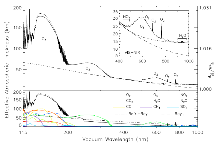
Figure 1.— Effective atmospheric thickness and effective planetary radius, R_eff (expressed in Earth radii, R_p), of a transiting Earth as a function of wavelength. The upper panel shows the overall spectrum from the UV to the NIR while the small insert panel zooms on the visible and NIR for clarity. Prominent spectral features are identified. The lower panel shows the effect of individual species (see Fig. 2 for details). In all panels, the solid and short-dashed lines are for solar minimum and solar maximum conditions, respectively. Furthermore, the dot-dashed and dashed lines show the individual contribution of Rayleigh scattering by N₂, O₂, Ar and CO₂, with and without the effect of refraction by these same species, respectively. See electronic edition of the Journal for a color version of this figure.

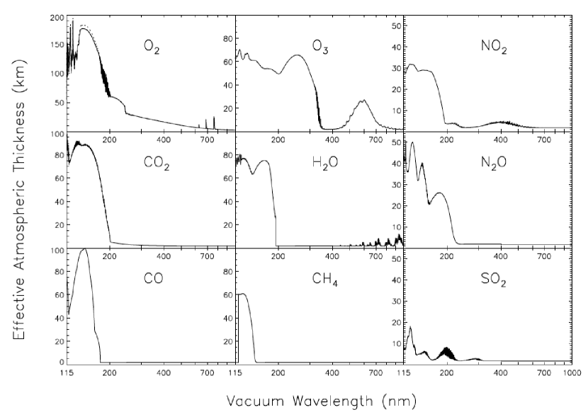
Figure 2.— Effective atmospheric thickness for each molecular species as a function of wavelength, assuming it is the only one with a non-zero opacity. Note the difference in scale on the y-axis: 200 km for O₂, 55 km for NO₂, N₂O, and SO₂, and 100 km elsewhere. O₂ and CO₂ curves also show the effect of Rayleigh scattering. The O₂ panel shows differences between solar minimum (solid line) and solar maximum (short-dashed line) conditions.

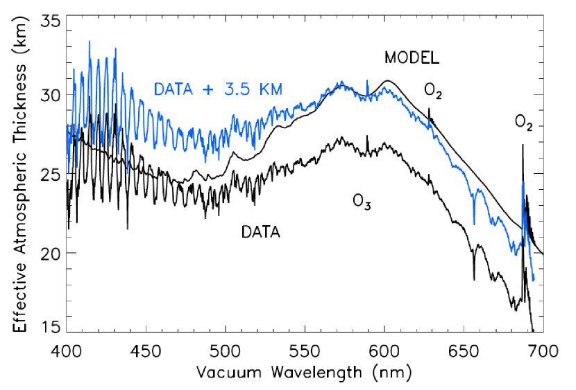
Figure 3.— Comparison of our model transiting Earth effective atmospheric thickness with the data of Vidal-Madjar et al. (2010). The data is also shown shifted by +3.5 km for ease of comparison. Note that the obvious oscillatory features on the short wavelength side of the data are due to uncorrected echelle spectrograph cross-order contamination and should be ignored.

Table 1UV - NIR model continuous absorption cross sections.

Species	Temperature of data (K)	Wavelength range (nm)	References
O2	303	115.0 - 179.2	Lu et al. (2010)
	300	179.2 - 203.0	Yoshino et al. (1992)
	298	203.0 - 240.5	Yoshino et al. (1988)
	298	240.5 - 294.0	Fally et al. (2000)
O3	298	110.4 - 150.0	Mason et al. (1996)
	298	150.0 - 194.0	Ackerman (1971)
	218	194.0 - 230.0	Brion et al. (1993)
	293, 273, 243, 223	230.0 - 1070.0	Bogumil et al. (2003)
NO2	298	15.5 - 192.0	Au & Brion (1997)
	298	192.0 - 200.0	Nakayama et al. (1959)
	298	200.0 - 219.0	Schneider et al. (1987)
	293	219.0 - 500.01	Jenouvrier et al. (1996) + Mérienne et al. (1995)
	293, 273, 243, 223	500.01 - 930.1	Bogumil et al. (2003)
CO	298	6.2 - 177.0	Chan et al. (1993)
CO2	300	0.125 - 201.6	Huestis & Berkowitz (2010)
H2O	298	114.8 - 193.9	Mota et al. (2005)
CH4	295	120.0 - 142.5	Chen & Wu (2004)
	295	142.5 - 152.0	Lee et al. (2001)
N2O	298	108.2 - 172.5	Zelikoff et al. (1953)
	302, 263, 243, 225, 194	172.5 - 240.0	Selwyn et al. (1977)
SO2	293	106.1 - 171.95	Manatt & Lane (1993)
	295	171.95 - 262.53	Wu et al. (2000)
	358, 338, 318, 298	262.53 - 416.66	Vandaele et al. (2009)

Table 2Parameters for Rayleigh cross section

Standard refractivity
Species	Wavelength range (nm)	References
N2	149 - 189	Griesmann & Burnett (1999)
	189 - 2060	Bates (1984)
O2	198 - 546	Bates (1984)
Ar	140 - 2100	Bideau-Mehu et al. (1981)
CO2	180 - 1700	Bideau-Mehu et al. (1973)
King correction factor
N2	$\geq$ 200	Bates (1984)
O2	$\geq$ 200	Bates (1984)
Ar	all	Bates (1984)
CO2	180 - 1700	Sneep & Ubachs (2005)

Note. — In unlisted spectral regions, quantities are assumed constant at the value of the closest wavelength for which data is available.

References

- Ackerman (1971) Ackerman, M. 1971, Mesospheric Models and Related Experiments, G. Fiocco, Dordrecht:D. Reidel Publishing Company, 149
- Au & Brion (1997) Au, J. W., & Brion, C. E. 1997, Chem. Phys., 218, 109
- Batalha et al. (2013) Batalha, N. M., Rowe, J. F., Bryson, S. T., et al. 2013, ApJS, 204, 24
- Bates (1984) Bates, D. R. 1984, Planet. Space Sci., 32, 785
- Bideau-Mehu et al. (1973) Bideau-Mehu, A., Guern, Y., Abjean, R., & Johannin-Gilles, A. 1973, Opt. Commun., 9, 432
- Bideau-Mehu et al. (1981) Bideau-Mehu, A., Guern, Y., Abjean, R., & Johannin-Gilles, A. 1981, J. Quant. Spec. Radiat. Transf., 25, 395
- Bogumil et al. (2003) Bogumil, K., Orphal, J., Homann, T., Voigt, S., Spietz, P., Fleischmann, O. C., Vogel, A., Hartmann, M., Bovensmann, H., Frerick, J., & Burrows, J. P. 2003, J. Photochem. Photobiol. A.: Chem., 157, 167
- Brion et al. (1993) Brion, J. Chakir, A., Daumont, D., Malicet, J., & Parisse, C. 1993, Chem. Phys. Lett., 213, 610
- Chan et al. (1993) Chan, W. F., Cooper, G., & Brion, C. E. 1993, Chem. Phys., 170, 123
- Chen & Wu (2004) Chen, F. Z., & Wu, C. Y. R. 2004, J. Quant. Spec. Radiat. Transf., 85, 195
- COESA (1976) COESA (Committee on Extension to the Standard Atmosphere) 1976, U.S. Standard Atmosphere, Washington, D.C.:Government Printing Office
- Cox (2000) Cox, A. N. 2000, Allen’s Astrophysical Quantities, 4th ed., New York:AIP
- Des Marais et al. (2002) Des Marais, D. J., Harwit, M. O., Jucks, K. W., Kasting, J. F., Lin, D. N. C., Lunine, J. I., Schneider, J., Seager, S., Traub, W. A., & Woolf, N. J. 2010, Astrobiology, 2, 153
- Ehrenreich et al. (2006) Ehrenreich, D., Tinetti, G., Lecavelier des Etangs, A., Vidal-Madjar, A., & Selsis, F. 2006, A&A, 448, 379
- Fally et al. (2000) Fally, S., Vandaele, A. C., Carleer, M., Hermans, C., Jenouvrier, A., Mérienne, M.-F., Coquart, B., & Colin, R. 2000, J. Mol. Spectrosc., 204, 10
- García Muñoz et al. (2012) García Muñoz, A., Zapatero Osorio, M. R., Barrena, R., Montañés-Rodríguez, P., Martín, E. L., & Pallé, E. 2012, ApJ, 755, 103
- Goldsmith (1963) Goldsmith, W. W. 1963, Icarus, 2, 341
- Greismann & Burnett (1999) Griesmann, U., & Burnett, J. H. 1999, Optics Letters, 24, 1699
- Hedelt et al. (2013) Hedelt, P., von Paris, P., Godolt, M., Gebauer, S., Grenfell, J. L., Rauer, H., Schreier, F., Selsis, F., & Trautmann, T. 2013, A&A, submitted (arXiv:astro-ph/1302.5516)
- Hedin (1987) Hedin, A. E. 1987, J. Geophys. Res., 92, 4649
- Huestis & Berkowitz (2010) Huestis, D. L. & Berkowitz, J. 2010, Advances in Geosciences, 25, 229
- Jenouvrier et al. (1996) Jenouvrier, A., Coquart, B., & Mérienne, M. F. 1996, J. Atmos. Chem., 25, 21
- Johnson et al. (1995) Johnson, D. G., Jucks, K. W., Traub, W. A., & Chance, K. V. 1995, J. Geophys. Res., 100, 3091
- Kaltenegger & Traub (2009) Kaltenegger, L., & Traub, W. A. 2009, ApJ, 698, 519
- Kaltenegger et al. (2010a) Kaltenegger, L., Selsis, F., Friedlund, M., Lammer, H., et al. 2010a, Astrobiology, 10, 89
- Kaltenegger et al. (2010b) Kaltenegger, L., Henning, W. G., & Sasselov, D. D. 2010b, AJ, 140, 1370
- Lee et al. (2001) Lee, A. Y. T., Yung, Y. L., Cheng, B. M., Bahou, M., Chung, C.-Y., & Lee, Y. P. 2001, ApJ, 551, L93
- Lodders & Fegley, J. (1998) Lodders, K., & Fegley, Jr., B. 1998, The Planetary Scientist’s Companion, New York:Oxford University Press
- Lu et al. (2010) Lu, H.-C., Chen, K.-K., Chen, H.-F., Cheng, B.-M., & Ogilvie, J. F. 2010, A&A, 520, A19
- Manatt & Lane (1993) Manatt, S. L., & Lane, A. L. 1993, J. Quant. Spec. Radiat. Transf., 50, 267
- Mason et al. (1996) Mason, N. J., Gingell, J. M., Davies, J. A., Zhao, H., Walker, I. C., & Siggel, M. R. F. 1996, J. Phys. B: At. Mol. Opt. Phys., 29, 3075
- Mérienne et al. (1995) Mérienne, M. F., Jenouvrier, A., & Coquart, B. 1995, J. Atmos. Chem., 20, 281
- Mota et al. (2005) Mota, R., Parafita, R., Giuliani, A., Hubin-Franskin, M.-J., Lourenço, J. M. C., Garcia, G., Hoffmann, S. V., Mason, M. J., Ribeiro, P. A., Raposo, M., & Limão-Vieira, P. 2005, Chem. Phys. Lett., 416, 152
- Nakayama et al. (1959) Nakayama, T., Kitamura, M. T., & Watanabe, K. 1959, J. Chem. Phys., 30, 1180
- Pallé et al. (2009) Pallé, E., Zapatero Osorio, M. R., Barrena, R., Montañés-Rodríguez, P., & Martín, E. L. 2009, Nature, 459, 814
- Rauer et al. (2011) Rauer, H., Gebauer, S., von Paris, P., Cabrera, J., Godolt, M., Grenfell, J. L., Belu, A., Selsis, F., Hedelt, P., & Schreier, F. 2011, A&A, 529, A8
- Rees (1989) Rees, M. H. 1989, Physics and Chemistry of the Upper Atmosphere, 1st ed., Cambridge:Cambridge University Press
- Schneider et al. (1987) Schneider, W., Moortgat, G. K., Burrows, J. P., & Tyndall, G. S. 1987, J. Photochem. Photobiol., 40, 195
- Selwyn et al. (1977) Selwyn, G., Podolske, J., & Johnston, H. S. 1977, Geophys. Res. Lett., 4, 427
- Sidis & Sari (2010) Sidis, O., & Sari, R. 2010, ApJ, 720, 904
- Sneep & Ubachs (2005) Sneep, M. & Ubachs, W. 2005, J. Quant. Spec. Radiat. Transf., 92, 293
- Snellen et al. (2013) Snellen, I., de Kok, R., Le Poole, R., Brogi, M., & Birkby, J. 2013, ApJ, submitted (arXiv:astro-ph/1302.3251)
- Traub & Jucks (2002) Traub, W. A., & Jucks, K. W. 2002, AGU Geophysical Monograph Ser. 130, Atmospheres in the Solar System: Comparative Aeronomy, M. Mendillo, 369
- Traub & Stier (1976) Traub, W. A., & Stier, M. T. 1976, Appl. Opt., 15, 364
- Vandaele et al. (2009) Vandaele, A. C., Hermans, C., & Fally, S. 2009, J. Quant. Spec. Radiat. Transf., 110, 2115
- Vidal-Madjar et al. (2010) Vidal-Madjar, A., Arnold, A., Ehrenreich, D., Ferlet, R., Lecavelier des Etangs, A., Bouchy, F., et al. 2010, A&A, 523, A57
- Wu et al. (2000) Wu, C. Y. R., Yang, B. W., Chen, F. Z., Judge, D. L., Caldwell, J., & Trafton, L. M. 2000, Icarus, 145, 289
- Yoshino et al. (1988) Yoshino, K., Cheung, A. S.-C., Esmond, J. R., Parkinson, W. H., Freeman, D. E., Guberman, S. L., Jenouvrier, A., Coquart, B., & Mérienne, M. F. 1988, Planet. Space Sci., 36, 1469
- Yoshino et al. (1992) Yoshino, K., Esmond, J. R., Cheung, A. S.-C., Freeman, D. E., & Parkinson, W. H. 1992, Planet. Space Sci., 40, 185
- Zelikoff et al. (1953) Zelikoff, M., Watanabe, K., & Inn, E. C. Y. 1953, J. Chem. Phys., 21, 1643