Local spin relaxation within the random Heisenberg chain

Abstract

Finite–temperature local dynamical spin correlations $S_{nn}(\omega)$ are studied numerically within the random spin–$1/2$ antiferromagnetic Heisenberg chain. The aim is to explain measured NMR spin–lattice relaxation times in BaCu_2(Si_0.5Ge_0.5)_2O_7, which is the realization of a random spin chain. In agreement with experiments we find that the distribution of relaxation times within the model shows a very large span similar to the stretched–exponential form. The distribution is strongly reduced with increasing $T$, but stays finite also in the high–$T$ limit. Anomalous dynamical correlations can be associated to the random singlet concept but not directly to static quantities. Our results also reveal the crucial role of the spin anisotropy (interaction), since the behavior is in contrast with the ones for XX model, where we do not find any significant $T$ dependence of the distribution.

One–dimensional (1D) quantum spin systems with random exchange couplings reveal interesting phenomena fundamentally different from the behavior of ordered chains. Since the seminal studies of antiferromagnetic (AFM) random Heisenberg chains (RHC) by Dasgupta and Ma ma1979 ; dasgupta1980 using the renormalization–group approach and further development by Fisher fisher1994 , it has been recognized that the quenched disorder of exchange couplings $J$ leads at lowest energies to the formation of random singlets with vanishing effective $\tilde{J}$ at large distances. The consequence for the uniform static susceptibility $\chi^{0}$ is the singular Curie–type temperature ($T$) dependence, dominated by nearly uncoupled spins at low–$T$ and confirmed by numerical studies of model systems hirsch1980 , as well by measurements of $\chi^{0}(T)$ on the class of materials being the realizations of RHC physics, in particular the mixed system BaCu_2(Si_1-xGe_x)_2O_7 zheludev2007 ; shiroka2011 ; shiroka2012 .

Recent measurements of NMR spin–lattice relaxation times $T_{1}$ in BaCu_2(Si_0.5Ge_0.5)_2O_7 shiroka2011 reveal a broad distribution of different $T_{1}$ resulting in a nonexponential magnetization decay being rather of a stretched–exponential form. In connection to this the most remarkable is the strong $T$ dependence of the $T_{1}$ span becoming progressively large and the corresponding distribution non–Gaussian at low–$T$. It is evident that in a random system $T_{1}$, which is predominantly testing the local spin correlation function $S_{nn}(\omega\to 0)$, becomes site $n$ dependent and we are therefore dealing with the distribution of $T_{1n}$ leading to a nonexponential magnetization decay.

Theoretically the behavior of dynamical spin correlations in RHC has not been adequately addressed so far. There is (to our knowledge) no established model result and moreover no clear prediction for the behavior of dynamical ($\omega\neq 0$) spin correlations at $T>0$ in RHC. It seems plausible that the low–$T$ behavior should follow from the random–singlet concept and its scaling properties, discussed within the framework of the renormalization–group approaches dasgupta1980 ; fisher1994 ; westerberg1997 ; motrunich2001 . Still, the relation to singular static correlations as evidenced, e.g., by $\chi^{0}(T)$ diverging at $T\to 0$, and low- $\omega$ dynamical correlations is far from clear.

One open question is also the qualitative similarity to the behavior of the random anisotropic XX chain invoked in several studies bulaevskii1972 ; hirsch1980 ; westerberg1997 ; motrunich2001 . The latter system is equivalent to more elaborated problem of noninteracting (NI) spinless fermions with the off–diagonal (hopping) disorder theodorou1976 ; eggarter1978 .

In the following we present results for the dynamical local spin correlation function $S_{nn}(\omega)$, in particular for its limit $s=S_{nn}(\omega\to 0)$ relevant for the NMR $T_{1}$, within the AFM RHC model for $T>0$, obtained using the numerical method based on the density–matrix renormalization group (DMRG) approach kokalj2009 . At high $T\geq J$, distribution of $s$ reveals a modest but finite width qualitatively similar both for the isotropic and the XX chain. On the other hand, the low–$T$ variation established numerically is essentially different. While for the XX chain there is no significant $T$ dependence, results for the isotropic case reveal at low $T\ll J$ a very large span of $s$ values and corresponding $T_{1n}$, qualitatively and even quantitatively consistent with NMR experiments shiroka2011 .

We study in the following the 1D spin–$1/2$ model representing the AFM RHC,

$$H=\sum_{i}J_{i}\left(S^{x}_{i}S^{x}_{i+1}+S^{y}_{i}S^{y}_{i+1}+\Delta S^{z}_{i}S^{z}_{i+1}\right)\,,$$ (1)

where $J_{i}$ are random and we will assume their distribution as uncorrelated and uniform in the interval $J-\delta J\leq J_{i}\leq J+\delta J$, with the width $\delta J<J$ as the parameter. In the following we will consider predominantly the isotropic case $\Delta=1$, but as well the anisotropic XX case with $\Delta=0$. The chain is of the length $L$ with open boundary conditions (o.b.c.) as useful for the DMRG method. We further on use $J=1$ as the unit of energy as well as $\hbar=k_{B}=1$.

Our aim is to analyse the local spin dynamics in connection with the NMR spin–lattice relaxation shiroka2011 . In a homogeneous system the corresponding relaxation rate $1/T_{1}$ is expressed in terms of the $q$–dependent spin correlation function,

$$\frac{1}{T_{1}}=\sum_{q\alpha}A^{2}_{\alpha}(q)S^{\alpha\alpha}(q,\omega\to 0)\,,$$ (2)

where $A^{2}_{\alpha}(q)$ involve hyperfine interactions and NMR form factors shiroka2011 . In the Supplement supp we show that the dominant dynamical $\omega\to 0$ contribution at low–$T$ is coming from the regime $q\sim\pi$. Therefore the variation $A^{2}_{\alpha}(q)$ is not essential and the rate depends only on the local spin correlation function $1/T_{1}\propto S^{zz}_{\mathrm{loc}}(\omega\to 0)$. In a system with quenched disorder the relaxation time becomes site dependent, i.e. $T_{1n}$, hence we study in the following the local correlations $S_{nn}(\omega)$ and the distribution of local limits $s=S_{nn}(\omega\to 0)$ and related relaxation times $\tau=1/s$ where

$$S_{nn}(\omega)=\frac{1}{\pi}\mathrm{Re}\int\limits_{0}^{\infty}\mathrm{d}t\,{\rm e}^{\imath\omega t}\langle S^{z}_{n}(t)S^{z}_{n}(0)\rangle\,.$$ (3)

In order to reduce finite–size effects we study large systems employing the finite–temperature dynamical DMRG (FTD–DMRG) kokalj2009 ; schollwock2005 ; prelovsek2013 method to evaluate the dynamical $S_{nn}(\omega)$, Eq. (3). To reduce edge effects we choose the local site $n$ to be in the middle of the chain, $n=L/2$. The distribution of $s$ is then calculated with $N_{r}\sim 10^{3}$ different realizations of the system with random $J_{i}$. More technical detail on the calculation can be found in the Supplement supp .

We start the presentation of results with typical examples of $S_{nn}(\omega)$. In Fig. 1 we show calculated spectra for system with $L=80$ sites, $T=0.5$, $\Delta=1$, and three different realizations of $J_{i}$, i.e. the homogeneous system with $J_{i}=1$ and two configurations with $\delta J=0.7$. Spectra for the uniform system are broad and regular at $\omega\sim 0$ agreeing with those obtained with other methods naef1999 , while $S_{nn}(\omega)$ for random case strongly depend apart from $\delta J$ also on the local $J_{i},i\sim n$. In particular, spectra with both $J_{n-1}$ and $J_{n}$ small have large amplitude at the relevant $\omega\sim 0$, while spectra with one large $J_{n-1}$ or $J_{n}$ have most of the weight at high–$\omega$ and small amplitude at $\omega\sim 0$ (elaborated further in the conclusions). For the following analysis it is important that $s=S_{nn}(\omega\to 0)$ can be extracted reliably.

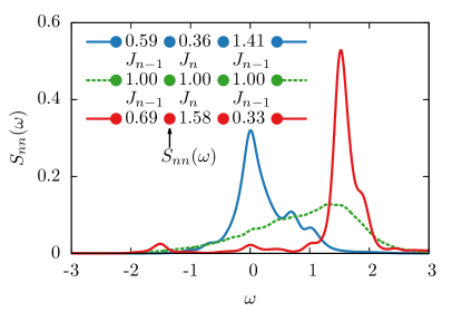
Figure 1: (Color online) Dynamical local spin correlations $S_{nn}(\omega)$ for different configurations of $J_{i}$. Shown are spectra for the homogeneous case $\delta J=0$ and two configurations with $\delta J=0.7$, calculated for $T=0.5$ and $L=80$ sites.

Results for $T\geq J$: Before displaying results for most interesting $T<J$ regime, we note that even at $T\gg J$ one cannot expect a well defined $\tau=\tau_{0}$ but rather a distribution of values. One can understand this by studying analytically local frequency moments within the high–$T$ expansion and using the Mori’s continued fraction representation mori1965 with the Gaussian–type truncation at the level of $l>3$ tommet1975 ; oitmaa1984 (see supp for more details). In the inset of Fig. 2 we present the high–$T$ result for $\mathrm{PDF}(s)$ and compare it with the numerical results evaluated for $T=1$. Several conclusions can be drawn from results presented on Fig. 2: (a) The agreement of PDF$(s)$ obtained via the analytical approach and numerical FTD–DMRG method is satisfactory having the origin in quite broad and featureless spectra $S_{nn}(\omega)$ at $T\geq J$. Still we note that median value of $s$ ($s_{\mathrm{med}}$) differ between both approaches and that for $T\gg J$ (unlike $T\leq J$) contribution of $q\to 0$ can become essential supp ; sandvik1997 . (b) PDF$(s)$ becomes quite asymmetric and broad for $\delta J\geq 0.5$. (c) Consequently, also the distribution of local relaxation times PDF$(\tau)$ has finite but modest width for $T\to\infty$. This seems in a qualitative agreement with NMR data for BaCu_2(Si_0.5Ge_0.5)_2O_7, where the width was hardly detected at high–$T$ shiroka2011 .

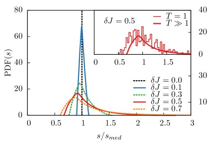
Figure 2: (Color online) Probability distribution function of local relaxation rates PDF$(s)$ at $T\gg 1$ evaluated using the moment expansion for different $\delta J$. Inset: Comparison of analytical and FTD–DMRG result for $\delta J=0.5$, $L=20$ with full basis and averaged over $N_{r}=10^{3}$ realizations.

Results for $T<J$: More challenging is the low–$T$ regime which we study using the FTD–DMRG method for typically $L=80$ and $N_{r}\sim 10^{3}$. Besides the isotropic case $(\Delta=1)$, we investigate for comparison also the XX model ($\Delta=0$). As the model of NI fermions with the off–diagonal disorder bulaevskii1972 ; theodorou1976 it can be easily studied via full diagonalization on much longer chains with $L\sim 16000$. PDF for $T<J$ can become very broad and asymmetric. Hence, we rather present results as the cumulative distribution $\mathrm{CDF}(x)=\int_{0}^{x}\mathrm{d}y\,\mathrm{PDF}(y)$. Further we rescale $x$ values to the median defined as $\mathrm{CDF}(x_{\mathrm{med}})=0.5$. Results for CDF$(s)$ are presented in Fig. 3. Note that $\mathrm{PDF}(\tau)=\mathrm{PDF}(s)/\tau^{2}$. Panels in Fig. 3 represent results for the isotropic case $\Delta=1$ with (a) fixed $T=0.2$ and varying $\delta J=0.1-0.9$, while in (b) $\delta J=0.7$ is fixed and $T=0.1-0.5$. Inset of Fig. 3b displays the $T$ dependence (for fixed $\delta J=0.7$) of CDF for the XX chain.

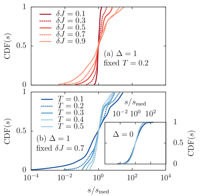
Figure 3: (Color online) Cumulative distribution function of $s$. Shown are FTD–DMRG results for $\Delta=1$: (a) for fixed $T=0.2$ and various $\delta J$, (b) for fixed $\delta J=0.7$ and various $T\leq 0.5$. Inset of (b):full diagonalization results for $\Delta=0$, $\delta J=0.7$ and various $T$.

We first note that within the XX chain CDF$(s)$ are essentially $T$ independent. This appears as quite a contrast to, e.g., static $\chi^{0}(T)$ which exhibits a divergence at $T\to 0$ hirsch1980 ; supp . Results for the isotropic case $\Delta=1$ in Figs. 3a,b are evidently different. The span in CDF becomes very large (note the logarithmic scale) either by increasing $\delta J$ at fixed $T$ or even more by decreasing $T$ at fixed $\delta J$. From the corresponding PDF one can calculate the relaxation function $R(t)=\int\mathrm{d}s\,\mathrm{PDF}(s){\rm e}^{-ts}$, which is in fact the quantity measured in the NMR as a time–dependent magnetization recovery shiroka2011 . As in experiment the large span in our results for low–$T$ can be captured by a stretched exponential form, $R(t)\approx\exp[-\left(t/\tau_{0}\right)^{\Gamma}]$, where $\Gamma$ and $\tau_{0}$ are parameters to be fitted for particular PDF$(s)$ and corresponding $R(t)$. It is evident that $\Gamma\ll 1$ means large deviations from the Gaussian–like form, and in particular very pronounced tails in PDF$(s)$, both for $s\gg s_{\mathrm{med}}$ as well as a singular variation for $s\to 0$. In the latter regime $1/\tau_{0}$ can deviate substantially from average of local $1/\tau$. It should be also noted that stretched exponential form, is the simplest one capturing the large span of $s$ values. It is also used in the experimental analysis shiroka2011 , but the corresponding PDF$(s)$ reveal somewhat enhanced tails for $s>s_{\mathrm{med}}$ relative to calculated ones in Fig. 3a,b, and the opposite trend for $s<s_{\mathrm{med}}$. This suggests possible improvements and description beyond stretched exponential form, which we leave as a future challenge. More details can be found in the Supplement supp .

Results for the fitted exponent $\Gamma(T)$ for $\Delta=1$ as extracted from numerical PDF$(s)$ for various $\delta J$ are shown in Fig. 4a. They confirm experimental observation shiroka2011 of increasing deviations from simple exponential variation ($\Gamma=1$) for $T\ll J$. While for $T>J$, $\Gamma\lesssim 1$ for modest $\delta J<0.7$, low–$T$ values can reach even $\Gamma<0.5$ at lowest reachable $T<0.1$. Note that in such a case values of $s$ are distributed over several orders of magnitude.

Of interest for the comparison with experiment is also the $T$ variation of fitted $1/\tau_{0}$. Results are again essentially different for $\Delta=0$ and $\Delta=1$. $\tau_{0}$ (as well $s_{\mathrm{med}}$) for $\Delta=0$ follows well the Korringa law $1/\tau_{0}\propto T$ for $T<0.5$, as usual for the system of NI fermions with a constant density of states (DOS) (divergent DOS at $E\to 0$ could induce a logarithmic correction). On the other hand, for the isotropic ($\Delta=1$) chain with no randomness $\tau_{0}=\tau$ it should follow $1/\tau\sim\mathrm{const.}$ for $T<J$ sandvik1995 ; naef1999 . Similar behavior is observed for weak disorder $\delta J=0.1$ as shown in Fig. 4b. However, with increasing randomness $\delta J$, $1/\tau_{0}$ becomes more $T$ dependent and increases with $T$. Such $T$ dependence in the RHC of $1/\tau_{0}$ is, although in agreement with experiment, in apparent contrast with diverging $\chi^{0}(T\to 0)$. This remarkable dichotomy between static and dynamical $\omega\to 0$ behaviour can be reconciled by the observation that in a random system $S(q,\omega\sim 0)$ reveals besides the regular part also a delta peak at $\omega=0$ (not entering $1/T_{1}$), which can be traced back to diagonal matrix elements supp being an indication of a nonergodic behaviour (at least at low–$T$). Note that more frequently studied static $S(q)$ (equal-time correlation) hoyos2007 represents a sum rule containing both parts. Also, the relation $\chi^{0}(T)=S(q=0)/T$ in spite of divergent $\chi(T\to 0)$ leads to vanishing $S(q=0)$ at $T\to 0$ only slower than linearly supp ; hoyos2007 .

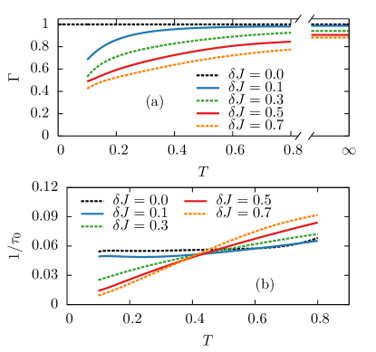
Figure 4: (Color online) (a) Exponent $\Gamma$ vs. $T$ obtained from PDF$(s)$ data for different $\delta J$ and isotropic case $\Delta=1$. (b) $T$ dependence of fitted $1/\tau_{0}$ for $\Delta=1$ and different $\delta J$.

As a partial summary of our results, we comment on the relation to the experiment on BaCu_2(Si_0.5Ge_0.5)_2O_7 zheludev2007 ; shiroka2011 . The spin chain is in this case assumed to be random mixture of two different values $J_{i}=280$ K, $580$ K, which correspond roughly to our $\delta J\simeq 0.6$ (fixing the same effective width) and $J=430$ K. Taking these values, our results for $\Gamma(T)$ as well as $1/\tau_{0}(T)$ agree well with experiment. In particular we note that at lowest $T\ll J$ our calculated $\Gamma\sim 0.5$ for $\delta J=0.6$ matches the measured one. Some discrepancy appears to be a steeper increase of measured $\Gamma(T)$ towards the limiting $\Gamma=1$ coinciding with observed very narrow PDF$(\tau)$ which remains of finite width in our results even for $T\to\infty$ as seen in Fig. 2. As far as calculated $1/\tau_{0}(T)$ vs. NMR experiment is concerned we note that taken into account the normalization of average $J$ disordered system reveals at $T\to 0$ smaller $1/\tau_{0}$ than a pure one consistent with the experiment shiroka2011 . In agreement with the experimental analysis is also strong $T$ variation of $1/\tau_{0}$ at low–$T$ in disordered system in contrast to a pure one.

Our results on the local spin relaxation $S_{nn}(\omega)$ and in particular its $T$ dependence cannot be directly explained within the framework of existing theoretical studies and scaling approaches to RHC dasgupta1980 ; fisher1994 ; motrunich2001 . Our study clearly shows the qualitative difference in the behavior of the XX chain and the isotropic RHC. While in the former model mapped on NI electrons, $T$ does not play any significant role on PDF$(s)$ as seen in inset of Fig. 3b, $\Delta=1$ case shows strong variation with $T\ll J$. It is plausible that the difference comes from the interaction and many–body character involved in the isotropic RHC. To account for that we design in the following a simple qualitative argument.

The behavior of $S_{nn}(\omega\sim 0)$ at low–$T$ is dominated by transitions between low–lying singlet and triplet states which become in a RHC nearly degenerate following the scaling arguments with effective coupling $\tilde{J}\to 0$ for more distant spins and reflected in diverging $\chi^{0}(T\to 0)$ supp ; dasgupta1980 ; hirsch1980 ; fisher1994 . Such transitions are relevant at $\omega\to 0$ behavior as presented in Fig. 1. Moreover, local $S_{nn}(\omega\sim 0)$ exhibit large spread due to the variations in the local environment. Let us for simplicity consider the symmetric Heisenberg model on four sites (with o.b.c.) with a stronger central bond $J_{2}\gg J_{1}=J_{3}$ and $J=(J_{1}+J_{2}+J_{3})/3$. It is then straightforward to show that the lowest singlet–triplet splitting is strongly reduced, i.e. $\Delta E\propto\eta^{2}J$ where $\eta=J_{1}/J_{2}$. Within the same model one can evaluate also the ratio between two different amplitudes of $S_{nn}(\omega\sim\Delta E)=A_{nn}\delta(\omega-\Delta E)$, on sites $n=1,2$ neighboring the weak and strong bond,

$$\frac{1}{W}=\frac{A_{22}}{A_{11}}=\frac{|\langle\Psi_{t}|S^{z}_{2}|\Psi_{s}\rangle|^{2}}{|\langle\Psi_{t}|S^{z}_{1}|\Psi_{s}\rangle|^{2}}\sim\eta^{2}\,.$$ (4)

The relation shows that the span between largest and smallest amplitudes increases as $W\propto 1/\eta^{2}\propto 1/\Delta E$. Continuing in the same manner the scaling procedure for AFM RHC dasgupta1980 ; fisher1994 for a long chain the smallest effective coupling between further spins $\tilde{J}$ vanishes at $T=0$ and $\Delta E\propto\tilde{J}\to 0$, so that one expects $W\to\infty$ for $T\to 0$. On the other hand, for $T>0$ the scaling should be cut off at $\tilde{J}\sim T$ at least for $\Delta=1$, finally leading to the strong $W(T)$ dependence ($W\propto 1/T$).

In the summary, we have reproduced qualitatively main experimental NMR results on mixed system BaCu_2(Si_0.5Ge_0.5)_2O_7 including anomalously wide distribution of relaxation rates, together with $T$ dependencies of experimental parameters ($1/\tau_{0}$, $\Gamma$) and provide microscopic explanation with the help of the random-singlet framework. Our qualitative conclusions on the RHC do not change by changing $S^{z}_{\mathrm{tot}}$ (adding finite field in the fermionic language) or even reducing $\Delta<1$ provided that $\Delta>0$ (see Supplement supp ). We also comment on striking difference between static and dynamic quantities and observed deviations from stretched exponential phenomenology.

SUPPLEMENTARY MATERIAL for “Local spin relaxation within random Heisenberg chain”

Appendix A I. NUMERICAL METHOD

In this section we present in more detail the numerical method, finite–temperature dynamical DMRG (FTD–DMRG). The method is a variation of a zero temperature ($T=0$) DMRG s_white1992 ; s_schollwock2005 , with targeting of the ground state or ground state density matrix $\rho_{0}=|0\rangle\langle 0|$ generalized to targeting of the finite–$T$ density matrix $\rho^{\beta}=\frac{1}{Z}\sum_{n}|n\rangle\textrm{e}^{-\beta H}\langle n|$, s_kokalj2009 ; s_kokalj2010 ; s_prelovsek2011 . Similar generalization is applied to targeting of the operator on the ground state. From such targets, the reduced density matrix is calculated and then truncated in the standard DMRG like manner for basis optimization. All quantities, that need to be evaluated at finite–$T$, are calculated with the use of finite–temperature Lanczos method (FTLM) s_jaklic2000 ; s_prelovsek2011 , which in FTD–DMRG replaces $T=0$ Lanczos method used in the standard DMRG algorithm.

The method is most efficient at low–$T$ and for low frequencies, where basis can be efficiently truncated and only small portion ($M$ basis states) of the whole basis for block can be kept. In this regime large system sizes can be reached. The truncation error becomes larger at higher–$T$, and one needs to either use larger $M$, or reduce system size, which is legitimate approach, since finite size effects are smaller at higher–$T$ due to reduced correlation lengths.

We typically keep $M\sim 200$ basis states in the DMRG block and use systems with length $L\sim 80$ at low $T<J/2$, while for $T>J/2$ smaller systems are employed down to $L\sim 20$, for which full basis can be used. We stress that randomness of $J_{i}$ reduces the truncation error since some larger values of $J_{i}$ induce strong tension for formation of a local singlet and therefore in turn reduces the entanglement on larger distances. Also the local operator, acting on the middle of the chain, where the local one site basis is not truncated, helps in this respect.

The quenched random $J_{i}$ are introduced into the DMRG procedure at the beginning of finite algorithm. Infinite algorithm is preformed for homogeneous system $J_{i}=J$ and the randomness of $J_{i}$ is introduced in the first sweep (see Fig. S1 for schematic presentation). In this way the preparation of the basis in the infinite algorithm is performed just once and for all realizations of $J_{i}$–s, while larger number of sweeps (usually $\sim 5$) is needed to converge the basis within the finite algorithm for random $J_{i}$. After finite algorithm local dynamical spin structure factor $S_{nn}(\omega)$ at desired $T$ is calculated for the site in the middle of the chain within measurements part of DMRG procedure.

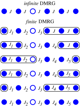
Figure S1: (Color online) Schematic ($L=6$) representation of the beginning of the sweeping method in finite–DMRG algorithm, in which randomness is introduced. Open circle represents site of a local operator used to calculated local spin correlation function in the measurement part of the DMRG method.

Any spectra on finite system consists of separate $\delta$–peaks, which we broaden by changing them into Gaussian with small broadening $\delta=0.05$ and in this way obtain a smooth spectra.

Since NMR relaxation rate is related to $S_{nn}(\omega\to 0)$, we are interested in the limit $\omega\to 0$, which should be contrasted with the singular $S_{nn}(\omega=0)$. In order to avoid the problem of diagonal elements and keeping $\omega\neq 0$ we perform the evaluation of $S_{nn}(\omega\to 0)$ in the magnetization sector $S^{z}_{\mathrm{tot}}=0$, which in terms of spinless fermions corresponds to the canonical ensemble (in the thermodynamic limit canonical and grand canonical give the same result) and we remove $\delta(\omega=0)$ peak (see also Section IV).

Diagonal elements are however essential when evaluating static uniform susceptibility $\chi^{0}(T)=\langle(S^{z}_{\mathrm{tot}})^{2}\rangle/(LT)$, which we show in Fig. S2. It has been argued s_hirsch1980 ; s_fisher1994 ; s_zheludev2007 , that in 1D random Heisenberg chain the density of low lying excitation is strongly increased, which is observed in diverging $\chi^{0}(T)$ for $T\to 0$. Our numerical results show similar behavior (see Fig. S2), which agrees also with experiment s_shiroka2011 ; s_masuda2004 .

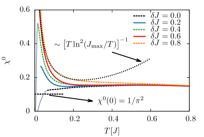
Figure S2: (Color online) Static spin susceptibility $\chi^{0}(T)$ vs. temperature $T$ for various randomness $\delta J$. For random system ($\delta J\neq 0$) $\chi^{0}(T)$ is strongly increased at low–$T$ and agrees with the random singlet s_fisher1994 prediction (black dotted line). Sudden drop of $\chi^{0}(T)$ at low–$T$ shown for $\delta J=0$ and $\delta J=0.4$ represents opening of finite–size gap, which is strongly reduced in the random (shown for $\delta J=0.4$) system. Results are obtained with the finite–temperature Lanczos method s_jaklic2000 ; s_prelovsek2011 on $L=24$ sites.

Increased number of low–lying excitations (see Fig. S2) also reduces the finite size effect, since, e.g., finite size gap is reduced, and in this way also the temperature $T_{\textrm{fs}}$, below which the finite size effects become important. Therefore, smaller $T$ can be numerically reached in a random system.

Appendix B II. HIGH–$T$ EXPANSION

The local spin correlation function can be related to the (local) dynamical spin susceptibility by relation

$$S_{nn}(\omega)\left[1-\exp(-\beta\omega)\right]=\chi_{nn}^{\prime\prime}(\omega)\,,$$ (S1)

with

$$\chi_{nn}(\omega)=\imath\int\limits_{0}^{\infty}\mathrm{d}t\,\mathrm{e}^{\imath\omega t}\langle[S^{z}_{n}(t),S^{z}_{n}(0)]\rangle\,.$$ (S2)

Taking the high–$T$ limit ($\beta\to 0$) of Eq. (S1) one gets $\beta S_{nn}(\omega)=\chi_{nn}^{\prime\prime}(\omega)/\omega$, which is so–called relaxation function - symmetric with respect to $\omega=0$, non–negative function. Note that due to symmetric form of relaxation function all odd frequency moments, $m_{ln}$, are equal to zero.

The local spin correlation function can by expressed by the Mori’s continued fraction representation s_mori1965 :

$$\hat{S}_{nn}(z=\imath\omega)=\cfrac{\delta_{0n}}{z+\cfrac{\delta_{1n}}{z+\cfrac{\delta_{2n}}{z+\cdots}}}\,,$$ (S3)

where coefficient $\delta_{ln}$ are cumulants of $S_{nn}(\omega)$, i.e. $\delta_{0n}=m_{0n}$, $\delta_{1n}=m_{2n}/m_{0n}$, $\delta_{2n}=m_{4n}/m_{2n}-m_{2n}/m_{0n}$. $m_{ln}$ are frequency moments of the local spectra, $m_{ln}=\int\mathrm{d}\omega\,\omega^{l}S_{nn}(\omega)$.

For $l>3$ we chose a truncation $\zeta_{n}=\delta_{3n}/(z+\dots)$, which assumes s_tommet1975 ; s_oitmaa1984 a Gaussian–like decay of correlation function, i.e. $\zeta_{n}=\sqrt{2/\pi}(\delta_{1n}+\delta_{2n})/\delta_{2n}^{3/2}$. The $S_{nn}(\omega)$ can be recovered from Eq. (S3) by the relation $S_{nn}(\omega)=\mathrm{Re}[\hat{S}_{nn}(z=\imath\omega)]/\pi$, leading to

$$S_{nn}(\omega)=\frac{1}{\pi}\frac{\zeta_{n}\delta_{0n}\delta_{1n}\delta_{2n}}{\left[\omega\zeta_{n}\left(\omega^{2}-\delta_{1n}-\delta_{2n}\right)\right]^{2}+\left(\omega^{2}-\delta_{1n}\right)^{2}}\,.$$ (S4)

Note that Eq. (S4) gives the first three nonzero ($l=0,2,4$) frequency moments $m_{ln}$ correctly, independent of a choice of $\zeta_{n}$.

Frequency moments $m_{ln}$ of $S_{nn}(\omega)$ can be evaluated analytically for $T=\infty$, e.g., $m_{0n}=\langle S^{z}_{n}S^{z}_{n}\rangle$, $m_{2n}=\langle[H,S^{z}_{n}][H,S^{z}_{n}]\rangle$, etc. For zero magnetization, $S^{z}_{\mathrm{tot}}=(L_{\uparrow}-L_{\downarrow})/2L=0$, where $L_{\uparrow}$ ($L_{\downarrow}$) is number of up (down) spins, the first three nonzero moments of the order of ${\cal O}(\beta)$ are:

$$m_{0n}=\frac{1}{4}\,,\qquad m_{2n}=\frac{J^{2}_{n-1}+J^{2}_{n}}{8}\,,$$

$$m_{4n}=\frac{1+\Delta^{2}}{32}\left(J^{2}_{n-2}J^{2}_{n-1}+J^{2}_{n}J^{2}_{n+1}\right)$$

$$+\frac{3+2\Delta^{2}}{32}\left(J^{4}_{n-1}+J^{4}_{n}\right)+\frac{7+2\Delta^{2}}{32}J^{2}_{n-1}J^{2}_{n}\,.$$ (S5)

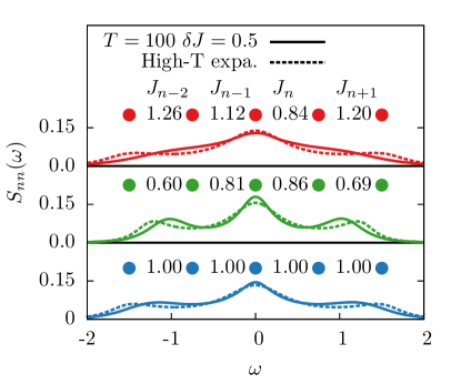
Figure S3: (Color online) Comparison of $S_{nn}(\omega)$ between analytical high–$T$ expansion result and numerical FTD–DMRG result ($L=20$, $T=100$, full basis) for three realization of $J_{i}$.

In Fig. S3 we present comparison of high–$T$ expansion result and FTD–DMRG result ($L=20$, $T=100$, full basis) for $S_{nn}(\omega)$ and three realizations of $J_{i}$. One can see that the agreement is good for actual finite size system. It should be, however, noted that $q\to 0$ contribution (leading to finite size corrections) can become essential for $T\gg J$ s_sandvik1997 .

As a final remark of this section we comment on the probability distribution function (PDF) of $s=S_{nn}(\omega\to 0)$ presented in Fig. 2 in the main text. Assuming the uniform distribution of $J_{i}$, $i=n-2,\cdots,n+1$ the PDF$(s)$ can be can be generated from expression

$$s=S_{nn}(\omega\to 0)=\frac{1}{\sqrt{8\pi^{3}}}\frac{\delta_{1n}+\delta_{2n}}{\delta_{1n}\delta_{2n}^{1/2}}\,.$$ (S6)

The PDF-s presented in Fig. 2 (main text) where obtained from $N_{r}=10^{6}$ realizations of $J_{i}$.

Appendix C III. FINITE MAGNETIC FIELD AND $\Delta=0.5$

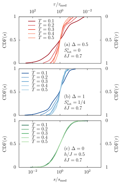
Figure S4: (Color online) Cumulative distribution function of relaxation rates $s$ and times $\tau=1/s$. Shown are FTD–DMRG results for various $T\leq 0.5$ and: (a) for $\Delta=0.5$, $S^{z}_{\mathrm{tot}}=0$ and $\delta J=0.7$, (b) for $\Delta=1$, $S^{z}_{\mathrm{tot}}=1/4$ and $\delta J=0.7$, while (c) are diagonalization results for $\Delta=0$, $\delta J=0.7$ and $h/J=0.5$.

In Fig. S4 we show that our main conclusions stay valid also in a more general case, such as for $\Delta=0.5<1$ and for finite magnetization ($S_{tot}^{z}=1/4$), where considerable $T$ dependence of distribution with large spread is observed. In the last panel of Fig. S4 we show that the distribution for noninteracting case (XX model) stays $T$ independent even in a finite magnetic field $h$ or for finite magnetization.

Appendix D IV. Wavevector resolved spin structure factor

Looking at the diverging uniform ($q=0$) susceptibility $\chi^{0}(T)$ as $T\to 0$ (Fig. S2) intuitively suggests large low–$q$ response and in turn increasing contribution of $S(q\sim 0,\omega)$ to the spin relaxation rate $1/T_{1}$ as $T\to 0$. This is not what is observed, since we see no increase of $1/\tau_{0}$ (Fig. 4b in the main text) as $T\to 0$, but instead $1/\tau_{0}$ decreases with decreasing $T$, which is in agreement also with experimental data (Ref. s_shiroka2011 , Fig. 3a).

This dichotomy can be partly understood by exploring the connection between static uniform spin susceptibility $\chi^{0}(T)$ with the static spin structure factor (equal-time correlation) $S(q)$, representing also the frequency integral of dynamical spin structure factor $S(q)=\int_{-\infty}^{\infty}\mathrm{d}\omega\,S(q,\omega)$. The connection $\chi^{0}(T)=S(q=0)/T$ together with the low–$T$ RG results (see Fig. S2) $\chi^{0}(T)=A/[T\ln^{2}(J_{\textrm{max}}/T)]$ leads to $S(q=0)=A/[\ln^{2}(J_{\textrm{max}}/T)]$. This shows that $S(q=0)$ goes to 0 as $T\to 0$ and is not diverging, rather its slow logarithmic approach to $0$ (in contrast to linear in $T$ decrease for homogeneous system). This is in agreement with results in Fig. 15 in Ref. s_hoyos2007 , which show that $S(q)$ at $T=0$ goes to 0 as $q\to 0$ and is only slightly increased by randomness for $q\sim 0$.

Another remarkable property of RHC can be seen in the difference between dynamic ($\omega>0$) properties, e.g. $S(q,\omega\to 0)$, and strictly $\omega=0$ contribution. This is shown in the lower panel of Fig. S5, which shows that $S(q,\omega)$ is singular at $\omega=0$ since it consists besides the continuous background (regular part) also of a distinct delta peak at $\omega=0$ (see Fig. S5b). This peak is non–dispersive and is the signature of non–ergodicity in the random system (absence of diffusion) at least for low–$T$. Similar peak is observed even in a random non–interacting electron system at finite–$T$ (not presented). In our analysis of spin relaxation for which $\omega\to 0$ is relevant, the $\omega=0$ peak was excluded (see Fig. S5c and also Section I above). Distinction between strictly $\omega=0$ and $\omega>0$ properties can be traced back to the difference between diagonal elements, e.g. $\langle(S^{z}_{tot})^{2}\rangle$ determining $\chi^{0}$ with only total spin $S>0$ (triplet) states contributing, and non–diagonal elements describing the transitions between, e.g. singlet and triplet states, which are relevant for dynamical ($\omega>0$) properties.

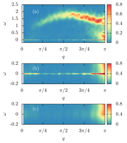
Figure S5: (Color online) (a) Wavevector resolved $S(q,\omega)$ for $\delta J=0.8$ and $T=0.1$ showing much larger weight at low–$\omega$ at $q\sim\pi$. Panel (b) show $S(q,\omega)$ for low $\omega$ where the non–dispersive $\omega=0$ delta peak is seen. The width of the peak is due to thew broadening used in the presentation. Panel (c) show low–$\omega$ $S(q,\omega)$ with removed $\omega=0$ delta peak.

D.1 IVa. Dominance of wavevectors $q\sim\pi$ in relaxation rate

By approximating NMR relaxation rate $1/T_{1}$ with local $S_{\textrm{loc}}(\omega\to 0)$, we neglected the effect of form factors ($A_{\alpha}^{2}(q)$, Eq. 2 in the main text), which is a good approximation since in the regime of our calculations the main contribution comes only from $q\sim\pi$. To show this, we present $S(q,\omega)$ in Fig. S5, where it is evident that the main contribution at $\omega\to 0$ comes from $q\sim\pi$. This stays valid even in the low–$T$ regime, where $\chi^{0}(T)$ is already increased due to renormalization of $J$-s as observed in the RG flow. Randomness does in fact slightly reduces the contribution of $q\sim\pi$ and slightly increases the contribution of $q\sim 0$, but the transfer of weight is much too small to make $q\sim 0$ dominant. This is in agreement with finding for $S(q)$ shown in Fig. 15 in Ref. s_hoyos2007 , where even for very large randomness and $T=0$ the main contribution stays at $q\sim\pi$ similarly to the homogeneous system s_sandvik1995 . It also agrees with experimental observation and direct statement of the authors s_shiroka2011 , that there in no indication of important $q\sim 0$ contributions as, e.g., the d.c. field dependence of $1/T_{1}$, being indication of the absence of (anomalous) low–$q$ (diffusion) contribution.

D.2 IVb. Long–wavelength contributions

Our analysis of local $s$ was based on assumption that there is no singular contribution emerging from long–wavelength $q\to 0$ physics. Indeed, all our available data for $S^{zz}(q,\omega\to 0)$ for AFM RHC confirm that the dominant regime at low–$T$ is $q\sim\pi$. Still, $q\to 0$ regime needs further attention since it can lead at $T>J$ to a divergent $S_{nn}(\omega\to 0)\propto 1/\omega^{\alpha}$ either from the propagation (prevented by randomness in the RHC) in the homogeneous XX chain s_naef1999 (with $\alpha\to 0$) or even more as the consequence of the spin diffusion s_sirker2009 ($\alpha=1/2$). The latter can be realized at $T>0$ but vanishes at $T\to 0$ within the RHC s_theodorou1976 ; s_motrunich2001 . Our results so far indicate that in spite of possible $T>0$ diffusion its contribution to $S_{nn}(\omega\to 0)$ is unresolvable for reachable systems, as follows also from NMR experiments s_shiroka2011 where it can be directly tested via the magnetic field dependence of $T_{1}$.

Appendix E V. Binary disorder distribution

Concrete realization of a random system in Ref. s_shiroka2011 , namely BaCu_2(Si_0.5Ge_0.5)_2O_7, has binary disorder distribution with two exchange couplings, $J_{\text{Si}}=280\,[K]$ and $J_{\text{Ge}}=580\,[K]$, which is in contrast with our continuous disorder distribution model, motivated by a usual theoretical reference. Therefore the question arises, how different are the results for the binary distribution from our results. Here we argue that the results are qualitatively and even quantitatively very similar for both distributions. This was realized already by J. E. Hirsch s_hirsch1980 , who showed that arbitrary disorder distribution lead to the similar low–$T$ behaviour.

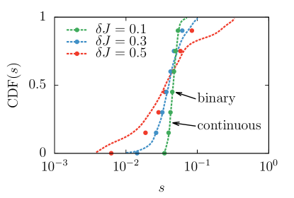
Figure S6: (Color online) Comparison of CDF-s for continuous and binary disorder distribution. Both distributions give almost the same CDF for small disorder, while for larger disorder they show only small quantitative difference. Note that the $x$–axis is not rescaled and both distributions would therefore give almost the same $1/\tau_{0}$. Plots are for $L=80$, $T=0.3$ and obtained with $N_{r}=10^{3}$ realizations.

To demonstrate the effect of binary distribution we show in Fig. S6 the comparison of relaxation rate CDF-s for continuous disorder distribution with the ones for binary disorder distribution with the same effective width. It is seen that the difference is small and largest for strongest disorder, where it still remains only quantitative, while for low disorder CDF-s are essentially the same for both disorder distributions. Therefore our results obtained with continuous distribution can easily be compared with measurements and they indeed agree qualitatively and to some extend even quantitatively with them (see main text).

Appendix F VI. Comments on stretched exponential

Using phenomenological stretched exponential form to fit experimental data on magnetization relaxation seems to be a common practice, which can be attributed to the fact that stretched exponential form can capture anomalously long tails in the distribution of the relaxation rates (normal distribution can not) and is at the same time very convenient for the fitting procedure. This immediately raises the question, how good this form really is for the description of experimental data and can it be motivated by some microscopic picture, e.g. model Hamiltonian.

In Fig. S7 we show our RHC model results for relaxation time distributions (PDF-s), which shows several important features when compared to the experimentally suggested stretched exponential forms (see Fig. 4 in Ref. s_shiroka2011 ). First one can see that the $T$ evolution is similar to the experimental one and more importantly at low–$T$ anomalously long tails (or large spread) in PDF appear, which can be captured with stretched exponential form and not with, e.g., normal (Gaussian) distribution. This could be the reason for the success of the stretched exponential form in the fitting procedures and its phenomenological description of experimental data.

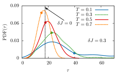
Figure S7: (Color online) Probability distribution function PDF($\tau$) for several temperatures and one randomness $\delta J=0.3$. These results should be compared with the shape of experimental ones in Fig. 4 in Ref. s_shiroka2011 . Temperature evolution of the distribution agrees with the experiment, as well as appearance of anomalously long tails of the distribution at low–$T$. Points correspond to fitted $\tau_{0}$ which shows similar $T$–dependence as experiment, while dashed vertical line corresponds to homogeneous ($\delta J=0$) model.

However, the description of our RHC model results with stretched exponential is not perfect as can be expected, and the most obvious deviations can be found in the long tails. E.g., for few specific value of $\Gamma$ analytical form of PDF-s is know s_lindsey1980 ; s_johnston2006 and for $\Gamma=0.5$ has a form

$$\mathrm{PDF}_{\Gamma=0.5}(s)=\frac{\exp\left[-1/\left(4\tau_{0}s\right)\right]}{\sqrt{4\pi\tau_{0}s^{3}}}\,.$$ (S7)

On Fig. S8 we compare our numerical result with $\Gamma=0.49$ (for $T=0.1$ and $\delta J=0.5$) with stretched exponential CDF obtained from Eq. (S7), $\mathrm{CDF}_{\Gamma=0.5}(s)=\mathrm{Erf}[1/(2\sqrt{s\,\tau_{0}})]$. We observe that the RHC model predicts longer (shorter) tails in the PDF for smaller (larger) $s$ than stretched exponential form. This is in turn reflected in the corresponding time dependent magnetization relaxation function (being Laplace transform of PDF) directly probed by experiment. One could, for example, from our PDF-s propose a new form (instead of stretched exponential) by approximating PDF-s with some function and performing its Laplace transform. This is however not trivial and we leave it as a motivation for future work. In this way obtained form is expected to describe experimental data better than stretched exponential, although differences might be small and experimental data with higher resolution might be needed.

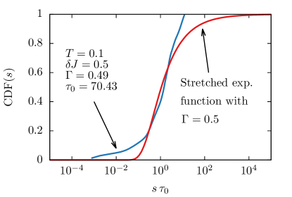
Figure S8: (Color online) One of more critical comparisons of our calculated CDF (blue line) to approximated stretched exponential form (red line) for $\Gamma\simeq 0.5$, for which stretched exponential distribution has particularly simple analytical form s_lindsey1980 ; s_johnston2006 .

References

- (1) S. R. White, Phys. Rev. Lett. 69, 2863 (1992).
- (2) U. Schollwöck, Rev. Mod. Phys. 77, 259 (2005).
- (3) J. Kokalj and P. Prelovšek, Phys. Rev. B 80, 205117 (2009).
- (4) J. Kokalj and P. Prelovšek, Phys. Rev. B 82, 060406(R) (2010).
- (5) For a recent review, see P. Prelovšek and J. Bonča, in Strongly Correlated Systems - Numerical Methods, edited by A. Avella and F. Mancini (Springer Series in Solid–State Sciences 176, Berlin, 2013), pp. 1–29.
- (6) J. Jaklič and P. Prelovšek, Adv. Phys. 49, 1 (2000).
- (7) D. Fisher, Phys. Rev. B 50, 3799 (1994).
- (8) J. E. Hirsch, Phys. Rev. B 22, 5355 (1980).
- (9) A. Zheludev, T. Masuda, G. Dhalenne, A. Revcolevschi, C. Frost, and T. Perring, Phys. Rev. B 75, 054409 (2007).
- (10) T. Shiroka, F. Casola, V. Glazkov, A. Zheludev, K. Prša, H.–R. Ott, and J. Mesot, Phys. Rev. Lett. 106, 137202 (2011).
- (11) T. Masuda, A. Zheludev, K. Uchinokura, J.-H. Chung, and S. Park, Phys. Rev. Lett. 93, 077206 (2004).
- (12) H. Mori, Prog. Theor. Phys. 34, 399 (1965).
- (13) T. N. Tommet and D. L. Huber, Phys. Rev. B 11, 1971 (1975).
- (14) J. Oitmaa, M. Plischke, and T. A. Winchester, Phys. Rev. B 29, 1321 (1984).
- (15) O. A. Starykh, A. W. Sandvik, and R. R. P. Singh, Phys. Rev. B 55, 14953 (1997).
- (16) J.A. Hoyos, A.P. Vieira, N. Laflorencie and E. Miranda, Phys. Rev. B 76, 174425 (2007).
- (17) A. W. Sandvik, Phys. Rev. B 52, R9831 (1995).
- (18) F. Naef, X. Wang, X. Zotos, and W. von der Linden, Phys. Rev B 60, 359 (1999).
- (19) J. Sirker, R. G. Pereira, and I. Affleck, Phys. Rev. Lett. 103, 216602 (2009).
- (20) G. Theodorou and M. H. Cohen, Phys. Rev. B 13, 4597 (1976).
- (21) O. Motrunich, K. Damle, and D. A. Huse, Phys. Rev. B 63, 134424 (2001).
- (22) O. Motrunich, K. Damle, and D. A. Huse, Phys. Rev. B 63, 134424 (2001).
- (23) C. P. Lindsey and G. D. Patterson, J. Chem. Phys. 73, 3348 (1980).
- (24) D. Johnston, Phys. Rev B 74, 184430 (2006).