Syntactic sensitive complexity for symbol-free sequence

Abstract

This work uses the L-system to construct a tree structure for the text sequence and derives its complexity [1]. It serves as a measure of structural complexity of the text. It is applied to anomaly detection in data transmission.

Keyword: text complexity, anomaly detection, structural complexity, rewriting rule, context-free grammar, L-system

1 Introduction

Complexity of the text has been developed with varying degrees of success, [2][3]. This work devised a novel measure based on L-system [1] that can compute the structural complexity of a text sequence. Given a text, we first transform it into a binary string. Then, use L-system to model the tree structure of this string and get its structural complexity. We will introduce how to use L-system to model the string in this section. The measure of complexity for the text sequence is included in the next section.

1.1 Transforming binary string into rewriting rules

The Lindenmayer system, or L-system, is a parallel rewriting system which was introduced by the biologist Aristid Lindenmayer in 1968. The major operation of L-system is rewriting. A set of rewriting rules, or productions, are operated to define a complex object by successively replacing parts of a simple initial object. The operations for a hierarchical tree can be represented by a set of rewriting rules. These rules can be further transformed into a bracketed string. A binary tree can be represented by a bracketed string and the tree can be restored from the string. This bracked string contains five symbols, $F$, $+$, $-$, $[$ , and $]$ . These symbols are defined in the following paragraph.

• $F$ denotes the current location of a tree node. It can be replaced by any word or be omitted.

• $+$  denotes the following string that represents the right subtree.

• $-$  denotes the following string that represents the left subtree.

• $[$  is pairing with $]$. “$[\ldots]$” denotes a subtree where “$\dots$” indicates all the bracketed string of its subtree.

Given a binary tree, the direct way to represent it with L-system is to construct rewriting rules that replace a tree with two smaller subtrees. An example is shown in Fig. 1. The left tree in Fig. 1 is expressed as $P\rightarrow[-F{T_{L}}][+F{T_{R}}]$. The right tree is expressed as $P\rightarrow[-F{T_{L}}][+F{T_{R}}]$ and ${T_{R}}\rightarrow[-F{T_{R_{L}}}][+F{T_{R_{R}}}]$. We see that the two rules, $P\rightarrow[-F{T_{L}}][+F{T_{R}}]$ and ${T_{R}}\rightarrow[-F{T_{R_{L}}}][+F{T_{R_{R}}}]$, are similar. The binary tree example in Fig.2 can be transformed into the set of rewriting rules in Table 1.

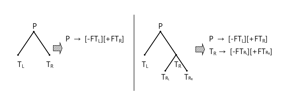
Figure 1: Rewriting rules for the two bracketed strings.

Fig.2 shows an example with four fixed tree elements representing the four 2-bit strings, { $00$, $10$, $01$, and $11$}. In this figure, every two leaves are combined into a small tree, and two small trees are combined into a bigger tree recursively. In this way, we can get a whole binary tree for a long binary string. Each node of the tree represents all its descendant string sections. The binary tree example in Fig.2 can be transformed into the set of rewriting rules in Table 1.

Figure 2: Binary string represented by binary tree.

Table 1: Rewriting Rules for the binary tree in Fig.2.

$P\rightarrow[-FT_{L}][+FT_{R}]$	$T_{R}\rightarrow[-FT_{R_{L}}][+FT_{R_{R}}]$
$T_{L}\rightarrow[-FT_{L_{L}}][+FT_{L_{R}}]$	$T_{R_{L}}\rightarrow[-FT_{R_{L_{L}}}][+FT_{R_{L_{R}}}]$
$T_{L_{L}}\rightarrow[-FT_{L_{L_{L}}}][+FT_{L_{L_{R}}}]$	$T_{R_{L_{L}}}\rightarrow[-F][+F]$
$T_{L_{L_{L}}}\rightarrow[-F][+F]$	$T_{R_{L_{R}}}\rightarrow[-F][+F]$
$T_{L_{L_{R}}}\rightarrow[-F][+F]$	$T_{R_{R}}\rightarrow[-FT_{R_{R_{L}}}][+FT_{R_{R_{R}}}]$
$T_{L_{R}}\rightarrow[-FT_{L_{R_{L}}}][+FT_{L_{R_{R}}}]$	$T_{R_{R_{L}}}\rightarrow[-F][+F]$
$T_{L_{R_{L}}}\rightarrow[-F][+F]$	$T_{R_{R_{R}}}\rightarrow[-F][+F]$
$T_{L_{R_{R}}}\rightarrow[-F][+F]$

1.2 Classifying rewriting rules into different sets

Two similarity definitions are used in classifying the rewriting rules.

Definition 1

Homomorphism in rewriting rules. We say rewriting rule $R_{1}$ and rewriting rule $R_{2}$ are homomorphic to each other if and only if they have the same structure.

Definition 2

Isomorphism on level X in rewriting rules. Rewriting rule $R_{1}$ and rewriting rule $R_{2}$ are isomorphic on depth $X$ if they are homomophic and their non-terminals are relatively isomophic on depth $X-1$. Isomorphic on level 0 indicates homomorphism.

After defining the similarity between rules by homomorphism and isomorphism, we can classify all the rules into different subsets where each subset has the same similarity relation. We will use the rule name as the class name. For example, we asign the terminal rewriting rule a class, “$C_{3}\rightarrow$ null”. Assign a rule linked to two terminals, “$C_{2}\rightarrow C_{3}C_{3}$”, here $C_{3}$ is the terminal class. After classification, we obtain a context free grammar set, which can be converted into an automata. After transforming the binary tree in Fig, 2 into the set of rewriting rules in Table 1, we can do classification and get the results listed in Table 2.

Table 2: Classification based on the similarity of rewriting rules. Several parameters for nodes and subtrees are attached to their symbols.

	Classification of Rules	Isomorphic Depth #2	Substring
$\left(n=10\right)$	Class #1 $\left(n_{1}=3\right)$	$n_{11}$      $\ a_{111}a_{112}$
		( 1)$C_{1}\rightarrow C_{1}C_{1}$
		$n_{12}$      $\ a_{121}a_{122}$	00100111
		( 1)$C_{1}\rightarrow C_{4}C_{3}$
		$n_{13}$      $\ a_{131}a_{132}$	00101101
		( 1)$C_{1}\rightarrow C_{4}C_{2}$
	Class #2 $\left(n_{2}=1\right)$	$n_{21}$      $\ a_{211}a_{212}$	1101
		( 1)$C_{2}\rightarrow C_{5}C_{7}$
	Class #3 $\left(n_{3}=1\right)$	$n_{31}$      $\ a_{311}a_{312}$	0111
		( 1)$C_{3}\rightarrow C_{7}C_{5}$
	Class #4 $\left(n_{4}=1\right)$	$n_{41}$      $\ a_{411}a_{412}$	0010
		( 2)$C_{4}\rightarrow C_{8}C_{6}$
	Class #5 $\left(n_{5}=1\right)$	$n_{51}$      $\ a_{511}a_{512}$	11
		( 2)$C_{5}\rightarrow C_{9}C_{9}$
	Class #6 $\left(n_{6}=1\right)$	$n_{61}$      $\ a_{611}a_{612}$	10
		( 2)$C_{6}\rightarrow C_{9}C_{10}$
	Class #7 $\left(n_{7}=1\right)$	$n_{71}$      $\ a_{711}a_{712}$	01
		( 2)$C_{7}\rightarrow C_{10}C_{9}$
	Class #8 $\left(n_{8}=1\right)$	$n_{81}$      $\ a_{811}a_{812}$	00
		( 2)$C_{8}\rightarrow C_{10}C_{10}$
	Class #9 $\left(n_{9}=1\right)$	$n_{91}$      $\ a_{911}a_{912}$	1
		( 8)$C_{9}\rightarrow$ null
	Class #10 $\left(n_{10}=1\right)$	$n_{10,1}$     $a_{10,11}a_{10,12}$	0
		( 8)$C_{10}\rightarrow$ null

1.3 Complexity for classified rules

The generating function of a context free grammar is defined in the following paragraph.

Definition 3

Generating function of a context free grammar.

1. Assume that there are $n$ classes of rules, $\{C_{1},C_{2},\dots,C_{n}\}$, and the class $C_{i}$ contains $n_{i}$ rules. Let $V_{i}\in\{C_{1},C_{2},\dots,C_{n}\}$, $U_{ij}\in\{R_{ij},i=1,2,\dots,n;$ $j=1,2,\dots,n_{i}\}$, and $a_{ijk}\in\{x:x=1,2,\dots,n\}$, where each $U_{ij}$ has the following form for a binary tree:

   $$\begin{array}[]{rl}U_{i1}&\rightarrow V_{a_{i11}}V_{a_{i12}}\\ U_{i2}&\rightarrow V_{a_{i21}}V_{a_{i22}}\\ \dots&\rightarrow\dots\\ U_{in_{i}}&\rightarrow V_{a_{i{n_{i}}1}}V_{a_{i{n_{i}}2}}\text{.}\end{array}$$

2. The generating function of $V_{i},V_{i}(z)$ has a form,

   $$V_{i}(z)=\frac{\sum\limits_{p=1}^{n_{i}}n_{ip}z^{k}V_{a_{ip1}}(z)V_{a_{ip2}}(z)}{\sum\limits_{q=1}^{n_{i}}n_{iq}}\text{.}$$

   If $V_{i}$ does not have any non-terminal, we set $V_{i}(z)=1$. The parameter $k$ is set to $1$, $k=1$, in [1]. An alternative setting is to weight the redundancy of rewriting rules by setting $k=1/n_{ip}$.

3. After formulating the generating function $V_{i}(z)$, we plan to find the largest value of $z,z^{max}$, where $V_{1}(z^{max})$ is convergent. Note that we will use $V_{1}$ to denote the function of the root node of the binary tree. After obtaining the largest value, $z^{max}$, of $V_{1}(z)$, we set $R=z^{max}$, where $R$ is the radius of convergence of $V_{1}(z)$. The complexity, $K_{0}$, of the binary tree is

   $$K_{0}=-\ln R\text{.}$$

4. Since computing the maximum value, $z^{max}$, directly is not feasible, we use iterations and region tests to accomplish the complexity. Rewrite the generating function in an iterative form,

   $$\begin{array}[]{rl}V_{i}^{m}(z^{\prime})&=\frac{\sum\limits_{p=1}^{n_{i}}n_{ip}z^{\prime k}V_{a_{ip1}}^{m-1}(z^{\prime})V_{a_{ip2}}^{m-1}(z^{\prime})}{\sum\limits_{q=1}^{n_{i}}n_{iq}}\quad;\text{ }m=1,2,3,...;\text{ }\mbox{and}\\ V_{i}^{0}(z^{\prime})&=1\text{.}\end{array}$$

5. The value of the function $V_{i}$ at a specific $z^{\prime}$ can be calculated by iterations of the form. In each iteration, calculate the values from $V_{i}^{0}(z^{\prime})$ to $V_{i}^{m}(z^{\prime})$. When $V_{i}^{m-1}(z^{\prime})=V_{i}^{m}(z^{\prime})$ is satisfied for all rules, we  stop the iteration. From experiences, we set $m=200$.

6. Now we can test whether $V_{i}(z^{\prime})$ is convergent or divergent at a value $z^{\prime}$. We use binary seaching to test the values between $0$ and $1$. In each test, when $V_{i}(z^{\prime})$ is convergent, we set a bigger value $z^{\prime}$ in the next test. When $V_{i}(z^{\prime})$ is divergent, we set a smaller value $z^{\prime}$ in the next test. We expect that this test will approach the radius, $R=z^{max}$, closely.

2 Complexity of encoded text

We show how to compute the complexity of the text. A text sequence is first transformed into a binary string by any giving encoding method. One can directly set each character be an integer and obtain a binary string for the text. For example, use the integer indexes, $1$ to $27$, to represent the 26 alphabets plus the space character. We use the term BIN to call this encoding method. This method is simple and doesn’t apply any sophisticated encoding algorithm. A different method, Lempel-Ziv-Welch (LZW), is also applied to encode the text. LZW is designed for lossless data compression and is a dictionary-based encoding [4]. In LZW, when certain substring appears frequently in the text, it will be saved in the dictionary. These two methods will be used in this work to accomplish the binary strings.

Before LZW processing, its dictionary contains all possible single characters of the text. LZW searches through the text sequence, successively, for a longer substring until it finds one that is not in the dictionary. Whenever LZW finds a substring that is in the dictionary, its index is retrieved from the dictionary and this index will replace the substring’s place in the encoded sequence. LZW will add a new substring to the dictionary and attach a new index to the substring. The last character of the newly replaced substring will be used as the next starting character to scan for new substrings. Longer strings are saved, successively, in the dictionary and made available for subsequent encoding. When LZW works on sequence with many repeated patterns, its compression efficiency is high.

For example, suppose there are only three characters “a”, “b”, “c” in the dictionary before we start searching. The indeices, “1”, “2”, and “3”, are used to represent them respectively. Giving a text “abcabcabc”, the substrings, “ab”, “bc”, “ca”, “abc”, “cab”, will be saved in the dictionary successively with their new assigned indeices, “4”, “5”, “6”, “7”, “8”. This string “abcabcabc” will be transformed into an array [1,2,3,4,6,5]. By using binary numbers, the array [1,2,3,4,6,5] can be transformed into a binary string ”001 010 011 100 110 101”.

Example

The article “The Declaration of Independence” is used as the text sequence. After removing all punctuation, the total number of characters are 7930. Apply the two encoding methods and obtain its two binary strings. We calculate the complexity every 512 bits along the string. Figure 3 shows that the complexity values of BIN are roughly fixed across the text sequence. The complexity values of LZW near the front end of the text are lower than those near the rear end of the text. Those lower valuses reveals the encoding features of LZW. Since the LZW dictionary saves a lot of regular patterns in the front end and absorbs the regularity, there will be no such regular patterns in the rear end. A string with high regularity has low complexity. So, the represented string near the rear end becomes much random with high complexity.

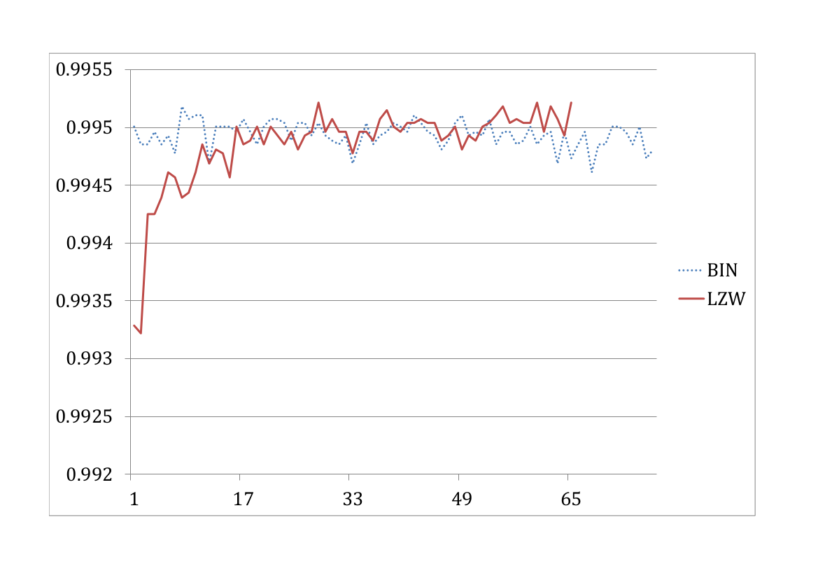
Figure 3: The complexity of the Declaration of Independence

3 Comparison with other Measures

Two other measures of complexity, topological entropy (TE) [2] and linguistic complexity (LC) are discussed and compared with the proposed method.

Topological entropy

An information function $A_{i}(s)$ is defined as,

$$A_{l}(s)=|\{u:|u|=l\text{ and }u\text{ is a distinct substring in }s\}|\text{,}$$

where $A_{i}(s)$ represents the total number of distinct substrings with length $l$ in the sequence $s$. The entropy [5] is defined as,

$$H_{l}(s)=\frac{log_{k}A_{l}(s)}{l}\text{,}$$

where $k$ is the size of all alphabets of the sequence. Since there are many values for $l$ and this definition can’t produce a single value of complexity for the whole sequence. A new definition [2] for the topological entropy is in the following paragraph.

Definition 4

Let $s$ be a finite sequence of length $|s|$ and $k$ be the size of alphabet, let $l$ be the unique integer such that

$$k^{l}+l-1\leq|s|\leq k^{l+1}+(l+1)-1$$

We use $s_{1}^{k^{l}+l-1}$ to represent the first $k^{l}+l-1$ letters of s.

$$H_{TE}(s):=\frac{log_{k}(A_{l}(s_{1}^{k^{l}+l-1}))}{l}$$

where $A_{l}(s_{1}^{k^{l}+l-1})$ is the number of distinct substrings with length $l$ in sequence $s_{1}^{k^{l}+l-1}$.

Linguistic complexity

Linguistic complexity [6, 8] is a measure of the vocabulary richness of a text. LC is defined as the ratio of the number of substrings presented in the string of interest to the maximum number of substrings of the same length string over the same alphabet. Thus, the more complex a text sequence, the richer its vocabulary, whereas a repetitious sequence has relatively lower complexity. Some notations are used in LC. Let $|s|$ be the length of the binary string $s$. Let $M_{l}(s)$ denote the maximal possible number of distinct substrings with length $l$, and $M_{l}(s)$ is equal to $min(2^{i},|s|-i+1)$. Let $M(s)$ be the sum of $M_{1}(s)$, $M_{2}(s)$,.., and $M_{|s|}(s)$. Let $A_{l}(s)$ be the actual number of distinct substrings with length $l$. Let $A(s)$ be the sum of $A_{1}(s)$, $A_{2}(s)$,…, and $A_{|s|}(s)$. Then, LC of the sequence $s$ is $A(s)/M(s)$.

For example, consider the binary string “$s_{1}:0111001100$”. The length of $s_{1}$ is equal to $|s_{1}|=10$. The $M(s_{1})$ value is $M(s_{1})=2+4+8+7+6+5+4+3+2+1=42$. Note that this value depends only on the length of the string and the alphabet size. We then use the suffix tree to calculate the actual number of distinct substrings, $A(s_{1})=38$. The LC value of $s_{1}$ is equal to $38/42=0.904762$.

We take another example “$s_{2}:0101010101$”. The length of $s_{2}$ is equal to $10$, and the value $M(s_{2})=42$ is also equal to $M(s_{1})$. The $A(s_{2})$ value $A(s_{2})=19$ is smaller than that of $A(s_{1})$. This is because $s_{2}$ is more regular. The LC of $s_{2}$ is equal to $19/42=0.45238$.

Comparison and analysis

Topological entropy focuses on only one subword length and computes its complexity. In contrast, linguistic complexity computes the complexity of all possible subword lengths. LC uses much more computations than that of TE. The proposed method uses the binary tree to represent a binary sequence that has a length of power of $2$. It reveals the structural information of the sequence.

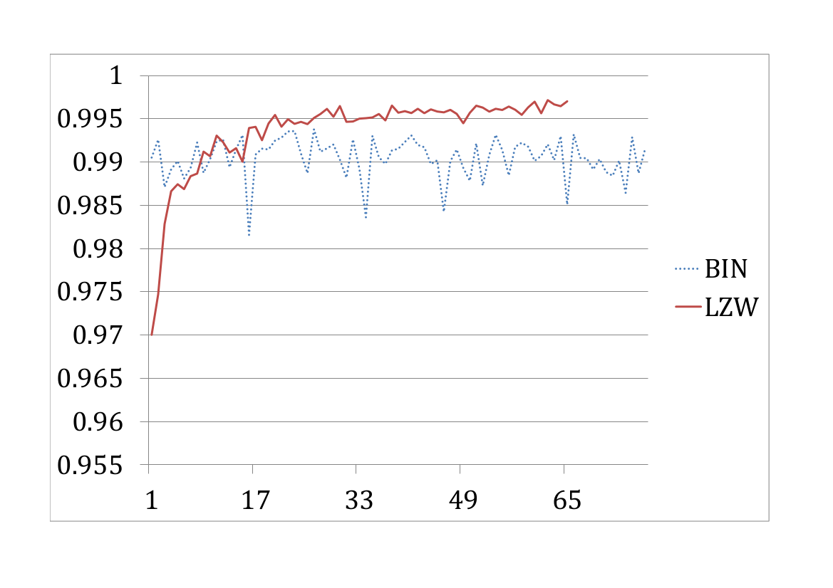
Figure 4: The linguistic complexity of the Declaration of Independence

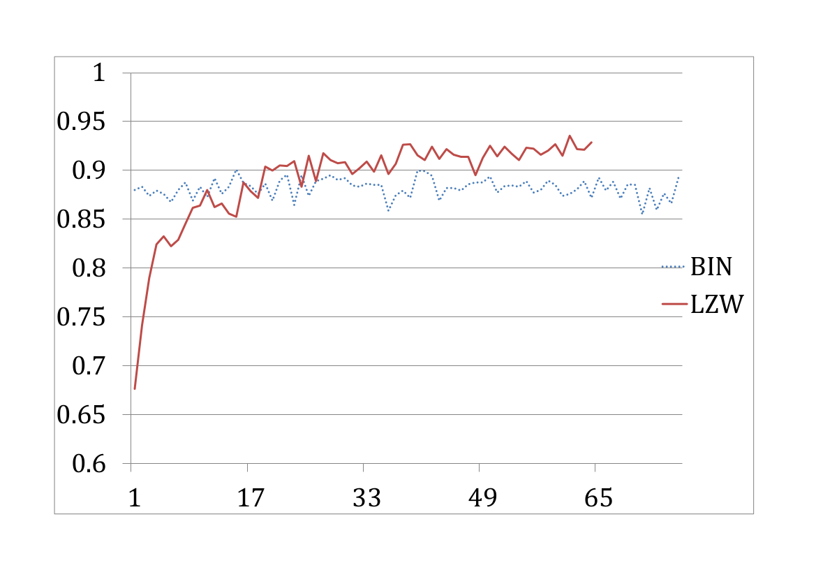
Figure 5: The topological entropy of the Declaration of Independence

Finally, we discuss some potential applications. The proposed complexity can be used to assist encoding and data compression. By monitoring the complexity of a text sequence, we can encode certain text sections of low complexity with better compression ratios and with fewer bits. We can also use the proposed complexity to detect anomaly in data transmission.

References

- [1] Liou, C.Y., Wu, T.H., Lee, C.Y.: Modeling complexity in musical rhythm. Complexity 15 (2010) 19–30
- [2] Koslicki, D.: Topological entropy of DNA sequences. Bioinformatics 27 (2011) 1061–1067
- [3] Tiño, P.: Spatial representation of symbolic sequences through iterative function systems. Systems, Man and Cybernetics, Part A: Systems and Humans, IEEE Transactions on 29 (1999) 386–393
- [4] Welch, T.A.: A technique for high-performance data compression. IEEE Computer 17 (1984) 8–19
- [5] Kirillova, O.V.: Entropy concepts and DNA investigations. Physics Letters A 274 (2000) 247–253
- [6] Gabrielian, A.E., Bolshoy, A.: Sequence complexity and DNA curvature. Computers & Chemistry 23 (1999) 263–274
- [7] Koukouvinos, C., Pillwein, V., Simos, D.E., Zafeirakopoulos, Z.: On the average complexity for the verification of compatible sequences. Inf. Process. Lett. 111 (2011) 825–830
- [8] Trifonov, E.: Making sense of the human genome. In: Structure and Methods: Human Genome Initiative and DNA Recombination. Volume 1. Adenine Press (1990) 69–77
- [9] Troyanskaya, O.G., Arbell, O., Koren, Y., Landau, G.M., Bolshoy, A.: Sequence complexity profiles of prokaryotic genomic sequences: A fast algorithm for calculating linguistic complexity. Bioinformatics 18 (2002) 679–688