Estimation of first passage time densities of diffusions processesthrough time-varying boundaries

Abstract.

In this paper, we develop a Monte Carlo based algorithm for estimating the FPT density of a time-homogeneous SDE through a time-dependent frontier. We consider Brownian bridges as well as localized Daniels curve approximations to obtain tractable estimations of the FPT probability between successive points of a simulated path of the process. Under mild assumptions, a (unique) Daniels curve local approximation can easily be obtained by explicitly solving a non-linear system of equations.

1. Introduction

Let $X$ be a time homogeneous diffusion process which is the unique (strong) solution of the following stochastic differential equation :

(1) $$dX\left(t\right)=\mu\left(X\left(t\right)\right)dt+\sigma\left(X\left(t\right)\right)dW\left(t\right),\>X\left(0\right)=x_{0}$$

if $S$ is a time dependent boundary, we are interested in estimating either the pdf or cdf of the first passage time (FPT) of the diffusion process through this boundary that is we will study the following random variable :

$$\tau_{S}=\inf\left\{t>0|X\left(t\right)=S\left(t\right)\right\}$$

In general, there is no explicit expression for the first passage-time density of a diffusion process through a time-varying boundary. To this date, only a few specific cases provide closed formed formulas for example when the process is gaussian and the boundary is of a Daniels’ curve type. Thus, we mainly rely on simulation techniques to estimate this density in a general setting.

The main goal of this work is to develop a computationally efficient algorithm that will provide reliable FPT density estimates. The paper is organized as follows. In section 2, we review existing techniques followed by the mathematical foundations leading to a novel algorithm. Finally, section 3 is devoted to various examples enabling us to evaluate the algorithm’s performance.

2. Monte Carlo simulation estimation

This is the simplest and best-known approach based on the law of large numbers. After fixing a time interval, basically we divide the latter into smaller ones, simulate a path of the process along those time points and, if it occurs, note the subinterval where the first upcrossing occurs. Generally, the midpoint of this subinterval forms the estimated first passage time of this simulated path. We repeat the process a large number of time to construct a pdf or cdf estimate of this stopping time.

Consider a Brownian motion $W$, a linear boundary $S\left(t\right)=\alpha+\beta t$, then for $\alpha>0$ and $T>0$, from standard theory the first passage time probability has an explicit form given by

$$P\left(\tau_{S}\leqslant T\right)=\Phi\left(-\frac{\alpha+\beta T}{\sqrt{T}}\right)+e^{-2\alpha\beta}\Phi\left(\frac{-\alpha+\beta T}{\sqrt{T}}\right)$$

where $\Phi$ denotes the cdf of a standard normal distribution.

Setting $\alpha=0.5$, $\beta=0.2$ and $T=1$, table 1 gives us estimates of the FPT probability with various number of simulated paths $N$ and time-step discretization $\Delta t$. Clearly, even in a simple case as this one, in order to have a suitable estimation of the true value $P\left(\tau_{S}\leqslant T\right)=0.5548$ we have to rely on a large number of paths and a very fine partition of the time interval.

Table 1. Monte Carlo estimates of the FPT probability of a Brownian motion through the boundary $S\left(t\right)=0.5+0.2t$

$P\left(\tau_{S}\leqslant 1.0\right)$	$\Delta t=10^{-2}$	$\Delta t=10^{-3}$	$\Delta t=10^{-4}$
$N=10^{4}$	0.5096	0.5407	0.5487
$N=10^{5}$	0.5102	0.5390	0.5506
$N=10^{6}$	0.5122	0.5412	0.5504

Another drawback of the crude Monte Carlo approach is that it tends to overestimates the true value of the first passage-time since an upcrossing may occur earlier in between simulated points of a complete path as illustrated in figure 1.

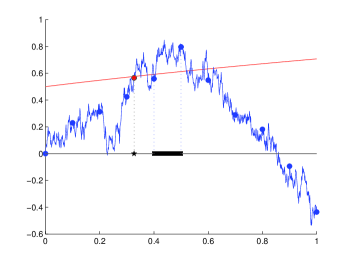
Figure 1. Undetected prior upcrossing through a basic Monte Carlo path simulation

2.1. Monte Carlo approach with intertemporal upcrossing simulations

Instead of continuously repeating the whole Monte Carlo procedure with an even finer interval partition to obtain better estimates, let us see how one could improve on the initial estimates without discarding the simulated paths.

An astute idea that have been put forward by several authors, is to ideally obtain the probability law of an upcrossing between simulated points, thus if $p_{k}$ is the probability of an upcrossing in the time interval $\left[t_{k},t_{k+1}\right]$, then one would simply generate a value $U_{k}$ taken from a uniform random variable on $\left[0,1\right]$ and assert that there is an upcrossing if $U_{k}\leqslant p_{k}$. Since the exact FPT probability of a diffusion bridge will more than often not be available, we need to consider an adequate estimation of this probability.

2.1.1. Diffusion bridge approximation

For each subinterval, one could consider simulating paths of approximate tied-down processes as proposed by Giraudo, Sacerdote and Zucca [1] where they basically used a Kloden Platen approximation scheme with order of convergence 1.5, or we could make use of more recent results from Lin, Chen and Mykland [2] or Sørensen and Bladt [3] to improve on the FPT probability estimates. Although all of these may constitute adequate approximations of the true FPT probability it may prove costly in computation time since these methods tantamounts to generating numerous simulations of bridge paths on successive subintervals for each of the original sample paths.

Another alternative, as first proposed in Strittmatter [4], is to consider that for a small enough interval, the diffusion part of the process should remain fairly constant and then consider a Brownian bridge approximation of the diffusion bridge and exploit known results on the FPT of Brownian bridges. For example Giraudo and Sacerdote [5] considered solving numerically the Volterra type integral equation linked to the generalized Brownian bridge FPT probability through a general time varying boundaries. Since a certain number of iterations may be needed to obtain adequate solutions of integral equations specific to each sample paths and successive subinterval this may sensibly increase computing time.

Finally, it is worth mentioning that all of the above methods could, in many cases, be improved significantly as far as accuracy is considered by first applying a Lamperti transform on both the original process and the frontier as described for example in Iacus [6].

Indeed , define

(2) $$F\left(x\right)=\int^{x}\frac{1}{\sigma\left(u\right)}du$$

and apply it on the original process and the time-varying boundary. Assuming that $F$ is one-to-one, then the original problem is equivalent to finding the FPT density of

$$\tau_{S^{*}}=\inf\left\{t>0|Y\left(t\right)=S^{*}\left(t\right)\right\}$$

where the new boundary is given by $S^{*}\left(t\right)=F\left(S\left(t\right)\right)$ and, by Itô’s formula, the diffusion process $Y$ follows the dynamic

(3) $$dY\left(t\right)=b\left(Y\left(t\right)\right)dt+dW\left(t\right),\;Y\left(0\right)=F\left(x_{0}\right)$$

where

$$b\left(t,Y\left(t\right)\right)=\frac{\mu\left(F^{-1}\left(Y\left(t\right)\right)\right)}{\sigma\left(F^{-1}\left(Y\left(t\right)\right)\right)}-\frac{1}{2}\frac{\partial\sigma}{\partial x}\left(F^{-1}\left(Y\left(t\right)\right)\right)$$

Since the diffusion part of the process $Y$ is constant, then the simple Brownian bridge will constitute a good approximation of the diffusion bridge.

2.1.2. Diffusion bridge approximation with local boundary approximation

In our approach, while still considering a Brownian bridge approximation of the diffusion bridges after a Lamperti transform as described previously, we propose to consider localized Daniels curve approximation of the time-varying boundary. Since explicit formulas of the first passage time probability are available in this case, one would readily get an adequate approximation of the true probability $p_{k}$. Furthermore, under mild assumptions, a (unique) Daniels curve approximation can easily be obtained by simply taking the endpoints of the segment and the value at midpoint (or another point of our choosing). Indeed, we will show that it leads to consider a non-linear system of three equations that can be explicitly solved.

Before describing our algorithm, we will need the following key results :

Proposition 1. Consider a Brownian bridge $W^{0,\Delta t}$ define on an time interval $\left[0,\Delta t\right]$ and $S$ a Daniels curve defined by

(4) $$S\left(t\right)=\frac{\alpha}{2}-\frac{t}{\alpha}\ln\left[\frac{\beta+\sqrt{\beta^{2}+4\gamma e^{-\alpha^{2}/t}}}{2}\right]$$

where $\alpha,\beta>0$, $\gamma\in R$ and $\lim_{t\rightarrow\Delta t}\beta^{2}+4\gamma e^{-\alpha^{2}/t}>0$, if $\tau_{S}=\inf\left\{0\leqslant t\leqslant\Delta t|W^{0,\Delta t}(t)=S(t)\right\}$ then

$$P\left(\tau_{S}\leqslant\Delta t\right)=\beta e^{-\frac{\alpha^{2}}{2\Delta t}}+\gamma e^{-\frac{2\alpha^{2}}{\Delta t}}$$

Proof. Apply Therom 3.4 of Di Nardo et al. [7].

Proposition 2. Let $\left[0,\Delta t\right]$ be a time interval, consider the points $\left(0,a\right)$, $\left(\Delta t/2,b\right)$,$\left(\Delta t,c\right)$ and set $A=e^{\frac{2a^{2}}{\Delta t}}$ $B=e^{-\frac{4\alpha b}{\Delta t}}$et $C=e^{-\frac{2ac}{\Delta t}}$. If

(5) $$\frac{1}{A^{2}}<\frac{B}{C}<\frac{1}{A}+\frac{\sqrt{A^{2}-1}}{A^{2}}$$

then there is a unique Daniels curve (4) passing through the three points with parameters

(6) $$\alpha=2a,\>\beta=\frac{A\left(A^{4}B^{2}-C^{2}\right)}{A^{3}B-C},\>\gamma=A^{4}C^{2}-\beta A^{3}C$$

Proof. The set of points generate the following non-linear system of equations :

$$\frac{\alpha}{2} = a$$

(7) $$\frac{\alpha}{2}-\frac{\Delta t}{2\alpha}\ln\left[\frac{\beta+\sqrt{\beta^{2}+4\gamma e^{-2\alpha^{2}/\Delta t}}}{2}\right] = b$$

$$\frac{\alpha}{2}-\frac{\Delta t}{\alpha}\ln\left[\frac{\beta+\sqrt{\beta^{2}+4\gamma e^{-\alpha^{2}/\Delta t}}}{2}\right] = c$$

obviously the first equation gives $\alpha=2a>0$, while simple algebraic manipulations on the last two equations lead us to solve the following linear system

$$\beta e^{\frac{\alpha^{2}-2\alpha b}{\Delta t}}+\gamma e^{-\frac{2\alpha^{2}}{\Delta t}} = e^{\frac{2\alpha^{2}-4\alpha b}{\Delta t}}$$

$$\beta e^{\frac{\alpha^{2}-\alpha b}{\Delta t}}+\gamma e^{-\frac{\alpha^{2}}{\Delta t}} = e^{\frac{\alpha^{2}-2\alpha b}{\Delta t}}$$

which can be rewritten in the form

$$\beta A^{6}B+\gamma = A^{8}B^{2}$$

$$\beta A^{3}C+\gamma = A^{4}C^{2}$$

since $A^{6}B-A^{3}C=A^{3}\left(A^{3}B-C\right)>0$ then there exists a unique solution given by :

$$\beta = \frac{A\left(A^{4}B^{2}-C^{2}\right)}{A^{3}B-C}$$

$$\gamma = A^{4}C^{2}-\beta A^{3}C$$

$$= A^{7}BC\left[\frac{C-AB}{A^{3}B-C}\right]$$

this would constitute the solution to the original system provided that $\beta>0$ and $\lim_{t\rightarrow\Delta t}\beta^{2}+4\gamma e^{-\alpha^{2}/t}>0$.

Notice first that $\frac{1}{A^{2}}<\frac{B}{C}\Rightarrow A^{4}B^{2}-C^{2}>0$ and therefore $\beta>0$ and if furthermore $\frac{B}{C}\leqslant\frac{1}{A}$ then $\gamma\geqslant 0$ and clearly $\lim_{t\rightarrow\Delta t}\beta^{2}+4\gamma e^{-\alpha^{2}/t}>0$ is satisfied. So if we assume now that $\frac{B}{C}>\frac{1}{A}$ then $\gamma<0$ , thus we need to verify that $\beta^{2}+\frac{4\gamma}{A^{2}}>0$ which is the case since

$$\beta^{2}+\frac{4\gamma}{A^{2}} = \frac{A^{2}\left(A^{4}B^{2}-C^{2}\right)^{2}}{\left(A^{3}B-C\right)^{2}}+4A^{5}BC\left[\frac{C-AB}{A^{3}B-C}\right]$$

$$= \frac{A^{2}}{\left(A^{3}B-C\right)^{2}}\left(\left(A^{4}B^{2}-C^{2}\right)^{2}+4A^{3}BC\left(C-AB\right)\left(A^{3}B-C\right)\right)$$

$$= \frac{A^{2}}{\left(A^{3}B-C\right)^{2}}\left(A^{4}B^{2}+C^{2}-2A^{3}BC\right)^{2}$$

The final step is to make sure that it solves the original system. Substituting back in (2.1.2), (where only positive square roots are involved), we see that is the case only if $A^{4}B^{2}+C^{2}-2A^{3}BC<0$, or equivalently

$$\left(\frac{B}{C}-\frac{1}{A}\right)^{2}<\frac{A^{2}-1}{A^{4}}$$

which is verified through (5). ∎

The FPT algorithm is described as follows :

1. Apply the Lamperti transform (2) to the original diffusion process (1) and frontier $S$ to obtain the new process (3) and boundary $S^{*}=F\left(S\left(t\right)\right)$

2. Select a time interval $\left[T_{l},T_{u}\right]$ and construct a partition $T_{l}=t_{0}<t_{1}<\ldots<t_{n}=T_{u}$

3. Initialize FPT vector counter to $\tau:=\left\{0,\ldots,0\right\}$

4. Initialize path counter to $k:=1$
   

   WHILE $k$ is less than $N$ the number of desired paths DO the following :
   

   1. Simulate a path of the process $\left\{Y\left(t_{1}\right),\ldots,Y\left(t_{n}\right)\right\}$

   2. Initialize subinterval counter to $i:=1$
      

      WHILE $i$ is less than $n$ the number of desired subintervals DO the following :
      

      1. IF $Y\left(t_{i}\right)\geqslant S^{*}\left(t_{i}\right)$ THEN set $i^{th}$ FPT vector component to $\tau_{i}:=\tau_{i}+1$ and path counter to $k:=k+1$, GO TO Step 5

      2. Set $\Delta:=t_{i}-t_{i-1}$, $a:=S\left(t_{i-1}\right)-Y\left(t_{i-1}\right)$, $b:=S\left(\frac{t_{i-1}+t_{i}}{2}\right)-Y\left(\frac{t_{i-1}+t_{i}}{2}\right)$,
         $c:=S\left(t_{i}\right)-Y\left(t_{i}\right)$, finally set $A$, $B$, $C$, $\alpha$, $\beta$ and $\gamma$ as in (6) of proposition 2

      3. IF $\frac{1}{A^{2}}<\frac{B}{C}<\frac{1}{A}+\frac{\sqrt{A^{2}-1}}{A^{2}}$ THEN set $c_{1}:=\beta$, $c_{2}:=\gamma$
         IF $\frac{1}{A^{2}}\geq\frac{B}{C}$ THEN set $c_{1}:=0$, $c_{2}:=A^{4}C^{2}$
         IF $\frac{B}{C}\geq\frac{1}{A}+\frac{\sqrt{A^{2}-1}}{A^{2}}$ THEN set $c_{1}:=2AC$ $c_{2}:=-A^{4}C^{2}$

      4. Set probability upcrossing to $p:=c_{1}e^{-\frac{\alpha^{2}}{2\Delta}}+c_{2}e^{-\frac{2\alpha^{2}}{\Delta}}$

      5. Generate a value $U$ taken from a uniform random variable

      6. IF $U\leq p$ THEN set $i^{th}$ FPT vector component to $\tau_{i}:=\tau_{i}+1$ and path counter to $k:=k+1$, GO TO Step 5, ELSE set $i:=i+1$, GO TO Step 7

Note that step 9 includes extreme cases where the middle point of the frontier in a subinterval may not be reached by a Daniels curve, thus we use the closest curve possible.

3. Examples

We will focus our examples on diffusion processes which paths can be simulated exactly. Therefore with known results on FPT density and bounds, it will allow us to better visualize the approximation error due essentially to the algorithm.

Example 1. Consider the following Ornstein-Uhlenbeck process and time varying boundary

$$dX\left(t\right) = \left(1.0-0.5X\left(t\right)\right)dt+dW\left(t\right),\>X\left(0\right)=1.6$$

$$S\left(t\right) = 2.0\left(1.0-\sinh\left(0.5t\right)\right)$$

This diffusion process is a Gauss-Markov process and according to Di Nardo et al. [7] the chosen boundary allows us to obtain an explicit FPT density given by

$$f\left(S\left(t\right),t\right)=\frac{e^{0.5t}}{\sinh\left(0.5t\right)}\varphi_{0}\left(S\left(t\right)\right)$$

where $\varphi_{0}$ is the probability density function of the Ornstein-Uhlenbeck process starting at $X\left(0\right)=0$.

Figure 2 compares the true FPT density with the empirical density histogram obtained through our algorithm using a time step discretization of 0.01 and 10 000 simulated paths. Furthermore, the algorithm gives us a FPT probability estimate of $0.9622$ over the whole interval compared to the true value of $0.9608$ representing a relative error of about $0.15\%$.

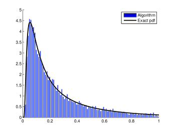
Figure 2. Ornstein-Uhlenbeck FPT pdf through the boundary $2.0\left(1.0-\sinh\left(0.5t\right)\right)$

Example 2. Consider the following geometric Brownian process and linear boundary

$$dX\left(t\right) = 5.0X\left(t\right)dt+2.5X\left(t\right)dW\left(t\right),\;X\left(0\right)=0.5$$

$$S\left(t\right) = 1.0+2.0t$$

By applying the Lamperti transform to both the process and boundary we obtain respectively

$$dY\left(t\right) = 0.75dt+dW\left(t\right),\>Y\left(0\right)=0.4\ln\left(0.5\right)$$

$$S^{*}\left(t\right) = 0.4\ln\left(1.0+2.0t\right)$$

As in example 1, this transformed diffusion process is also a Gauss-Markov process and, although the new frontier does not allow an explicit FPT density, using the deterministic algorithm in Di Nardo et al. [7] with a 0.01 time step discretization, we can obtain a reliable approximation.

Figure 2 compares the Di Nardo FPT density approximation with the empirical density histogram obtained through our algorithm using the same time step discretization with 10 000 simulated paths. In addition, the algorithm offers a FPT probability estimate of $0.8251$ over the whole interval agreeing with the actual value of $0.8258$ (a relative error of about $0.08\%$).

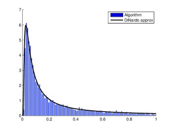
Figure 3. Geometric Brownian Motion FPT pdf through the boundary $1.0+2.0t$

Example 3. Consider the modified Cox-Ingersoll-Ross process and linear boundary

$$dX\left(t\right) = -0.5X\left(t\right)dt+\sqrt{1+X\left(t\right)^{2}}dW\left(t\right),\>X\left(0\right)=0$$

$$S\left(t\right) = 0.3+0.2t$$

By applying the Lamperti transform to both the process and boundary we obtain respectively

$$dY\left(t\right) = -\tanh\left(Y\left(t\right)\right)dt+dW\left(t\right),\>Y\left(0\right)=0$$

$$S^{*}\left(t\right) = \operatorname*{arcsinh}\left(0.3+0.2t\right)$$

As opposed to the preceding examples, this transformed diffusion process is not gaussian however using Beskos and Roberts’ [8] exact algorithm we can simulate exact sample paths. Although an explicit FPT density is not available, using results of Downes and Borovkov [9] we can, in this case, obtain the following lower and upper bounds:

$$f_{L}\left(S\left(t\right),t\right) = \frac{1}{t}\left(S\left(t\right)-\frac{0.2t}{\sqrt{1.09}}\right)\frac{e^{-0.5t}}{\cosh\left(S\left(t\right)\right)}\varphi_{W}\left(S\left(t\right)\right)$$

$$f_{U}\left(S\left(t\right),t\right) = \frac{1}{t}\left(S\left(t\right)-\frac{0.2t}{\sqrt{1.25}}\right)\frac{e^{0.5t}}{\cosh\left(S\left(t\right)\right)}\varphi_{W}\left(S\left(t\right)\right)$$

where $\varphi_{W}$ is the probability density function of a standard Brownian motion.

Figure 2 compares the FPT bounds with the empirical density histogram obtained through our algorithm using a 0.01 time step discretization starting initially with 15 000 simulations and obtaining 11 768 valid paths through the exact algorithm. Moreover, the algorithm suggests a FPT probability estimate of $0.7398$ over the whole interval which lies within the values $\int_{0}^{T}f_{L}\left(S\left(t\right),t\right)dt=0.6204$ and $\int_{0}^{T}f_{U}\left(S\left(t\right),t\right)dt=0.7673$.

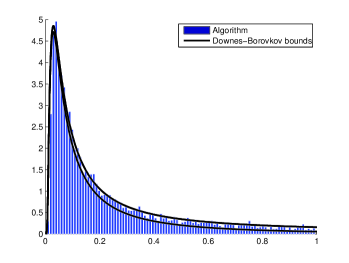
Figure 4. Modified CIR process FPT pdf through the boundary $0.3+0.2t$

References

- Giraudo, Sacerdote and Zucca [2001] Giraudo, M.T., Sacerdote, L. and Zucca, C., A Monte Carlo Method for the Simulation of First Passage Time of Diffusion Processes, Methodology and Computing in Applied Probability, Vol. 3, p. 215-231, 2001.
- Lin, Chen and Mykland [2010] Lin, M., Chen, R. and Mykland, P., On Generating Monte Carlo Samples of Continuous Diffusion Bridges, Journal of the American Statistical Association Vol. 105, No. 490, p. 820-838, 2010.
- Søorensen and Bladt [2013] Sørensen, M. and Bladt, M., Simple simulation of diffusion bridges with application to likelihood inference for diffusions, To appear in Bernoulli.
- Strittmatter [1987] Strittmatter, W., Numerical simulation of the mean first passage time, Preprint, University Freiburg, 1987.
- Giraudo and Sacerdote [1999] Giraudo, M.T., Sacerdote, L., An improved technique for the simulation of first passage times for diffusion processes, Communications in Statistics - Simulation and Computation, Vol. 28, No 4, p. 1135-1163, 1999.
- Iacus [2008] Iacus, S.M., Simulation and Inference for Stochastic Differential Equations, Springer, New York, 2008.
- Di Nardo et al. [2001] Di Nardo, E. et al., A Computational Approach to First Passage Time Problems for Gauss-Markov Processes, Advances in Applied Probability, Vol. 33, p. 453-482, 2001.
- Beskos and Roberts [2005] Beskos, A. and Roberts, G. O., Exact simulation of diffusions, Annals of Applied Probability, Vol. 15, No. 4, p. 2422-2444, 2005.
- Downes and Borovkov [2008] Downes, A.N. and Borovkov K., First Passage Densities and Boundary Crossing Probabilities for Diffusion Processes, Methodology and Computing in Applied Probability, Vo. 10, p. 621-644, 2008.