Algorithms of the LDA model

Jaka Špeh, Andrej Muhič, Jan Rupnik
Artificial Intelligence Laboratory
Jožef Stefan Institute
Jamova cesta 39, 1000 Ljubljana, Slovenia
e-mail: {jaka.speh, andrej.muhic, jan.rupnik}@ijs.si

ABSTRACT

We review three algorithms for Latent Dirichlet Allocation (LDA). Two of them are variational inference algorithms: Variational Bayesian inference and Online Variational Bayesian inference and one is Markov Chain Monte Carlo (MCMC) algorithm – Collapsed Gibbs sampling. We compare their time complexity and performance. We find that online variational Bayesian inference is the fastest algorithm and still returns reasonably good results.

1. INTRODUCTION

Nowadays big corpora are used daily. People often search through huge numbers of documents either in libraries or online, using web search engines. Therefore, we need efficient algorithms that enable us efficient information retrieval.

Sometimes appropriate documents are hard to find, especially if you do not have the exact title. One solution is to search using keywords. As many documents do not have keywords, we need to know what certain document is talking about. Therefore, we would like to tag documents with appropriate keywords by clustering them according to their topics.

As the size of corpus increases, manual annotation is not an option. We would like that computers process documents and find their topics automatically. That can be done using machine learning.

Probabilistic graphical models such as Latent Dirichlet Allocation (LDA) allow us to describe a document in terms of probabilistic distributions over topics, and these topics in terms of distributions over words. In order to obtain documents topics and corpus topics (distributions over words), we need to compute posterior distribution. Unfortunately, the posterior is intractable to compute and one must appeal to approximate posterior inference.

Modern approximate posterior inference algorithms fall into two categories: sampling approaches and optimization approaches. Sampling approaches are usually based on MCMC sampling. Conceptual idea of the methods is to generate independent samples from posterior and then reason about documents and corpus topics. Whereas optimization approaches are usually based on variational inference, also called Variational Bayes (VB) for Bayesian models. Variational Bayes methods optimize closeness, in Kullback-Leibler divergence, of simplified parametric distribution to the posterior.

In this paper, we compare one MCMC and two VB algorithms for approximating posterior distribution. In the subsequent sections, we formally introduce LDA model and algorithms. We study performance of algorithms and make comparisons between them. For training and testing set we use articles from Wikipedia. We show that Online Variational Bayesian inference is the fastest algorithm. However the accuracy is lower than in the other two, but the results are still good enough for practical use.

2. LDA MODEL

Latent Dirichlet Allocation [1] is a Bayesian probabilistic graphical model, which is regularly used in topic modeling. It assumes $M$ documents are build in a following fashion. First, a collection of $K$ topics (distributions over words) are drawn from a Dirichlet distribution, $\varphi_{k}\sim\mbox{Dirichlet}(\beta)$. Then for $m$-th document, we:

Figure 1. Plate notation of LDA.

1. Choose a topic distribution $\theta_{m}\sim\mbox{Dirichlet}(\alpha)$.

2. For each word $w_{m,n}$ in $m$-th document:

   1. choose a topic of the word

      $z_{m,n}\sim\mbox{Multinomial}(\theta_{m})$,

   2. choose a word $w_{m,n}\sim\mbox{Multinomial}(\varphi_{z_{m,n}})$.

LDA can be graphically presented using plate notation (Figure 1).

Probability of the LDA model is

$$p(\mathbf{w},\mathbf{z},\mathbf{\theta},\mathbf{\varphi}\mid\alpha,\beta)=$$

$$\prod_{k=1}^{K}p(\varphi_{k}|\beta)\prod_{m=1}^{M}\left(p(\theta_{m}|\alpha)\prod_{n=1}^{N_{m}}p(z_{m,n}|\theta_{m})p(w_{m,n}|\varphi_{z_{m,n}})\right).$$

We can analyse a corpus of documents by computing the posterior distribution of the hidden variables ($\mathbf{z},\mathbf{\theta},\mathbf{\varphi}$) given a document ($\mathbf{w}$). This posterior reveals latent structure in $\mathbf{w}$) brez oklepajev? the corpus that can be used for prediction or data exploration. Unfortunately, this distribution cannot be computed directly [1], and is usually approximated using Markov Chain Monte Carlo (MCMC) methods or variational inference.

3. ALGORITHMS

In the following subsections, we will derive one MCMC algorithm and two variational Bayes algorithms for the approximation of the posterior inference.

3.1. Collapsed Gibbs sampling

In the Collapsed Gibbs sampling we first integrate $\mathbf{\theta}$ and $\mathbf{\varphi}$ out.

$$p(\mathbf{z},\mathbf{w}\mid\alpha,\beta)=\int_{\mathbf{\theta}}\int_{\mathbf{\varphi}}p(\mathbf{z},\mathbf{w},\mathbf{\theta},\mathbf{\varphi}\mid\alpha,\beta)\;d\mathbf{\theta}\,d\mathbf{\varphi}.$$

The goal of Collapsed Gibbs sampling here is to approximate the distribution $p(\mathbf{z}\mid\mathbf{w},\alpha,\beta)$. Conditional probability $p(\mathbf{w}\mid\alpha,\beta)$ does not depend on $\mathbf{z},$ therefore Gibbs sampling equations can be derived from $p(\mathbf{z},\mathbf{w}\mid\alpha,\beta)$ directly. Specifically, we are interested in the following conditional probability

$$p(z_{m,n}\mid\mathbf{z}_{\lnot(m,n)},\mathbf{w},\alpha,\beta),$$

where $\mathbf{z}_{\lnot(m,n)}$ denotes all $z$-s but $z_{m,n}$. Note that for Collapsed Gibbs sampling we need only to sample a value for $z_{m,n}$ according to the above probability. Thus we only need thevalue of izbrisano probability mass function up to scalar multiplication. So, the distribution can be simplified [4, page 22] as:

(1) $$p(z_{m,n}=k\mid\mathbf{z}_{\lnot(m,n)},\mathbf{w},\alpha,\beta)\propto$$

$$\frac{n_{k,\lnot(m,n)}^{(v)}+\beta}{\sum_{v=1}^{V}(n_{k,\lnot(m,n)}^{(v)}+\beta)}\leavevmode\nobreak\ (n_{m,\lnot(m,n)}^{(k)}+\alpha),$$

where $n_{k}^{(v)}$ refers to the number of times that term $v$ has been observed with topic $k$, $n_{m}^{(k)}$ refers to the number of times that topic $k$ has been observed with a word of document $m$, and $n_{\;\cdot\;,\lnot(m,k)}^{(\;\cdot\;)}$ indicate that the $n$-th token in ., mogoče bolje eksplicitno $m$-th document is excluded from the corresponding $n_{k}^{(v)}$ or $n_{m}^{(k)}$.

Corpus and document topics can be obtained by [4, page 23]:

$$\varphi_{k,v}=\frac{n_{k}^{(t)}+\beta}{\sum_{v=1}^{V}(n_{k}^{(t)}+\beta)},\quad\theta_{m,k}=\frac{n_{m}^{(k)}+\alpha}{\sum_{k=1}^{K}(n_{m}^{(k)}+\alpha)}.$$

In Collapsed Gibbs sampling algorithm, we need to remember values of three variables: $z_{m,n}$, $n_{m}^{(k)},$ and $n_{k}^{(v)},$ and some sums of these variables for efficiency. The algorithm first initializes $\mathbf{z}$ and computes $n_{m}^{(k)}$, $n_{k}^{(v)}$ according to the initialized values. Then in one iteration of the algorithm we go over all words of all documents, sample values of $z_{m,n}$ according to Equation (1), and recompute $n_{m}^{(k)}$, $n_{k}^{(v)}$. Then one has to decide when (from which iteration/s) to take a sample or samples and which criteria to choose to check if Markov chain has converged.

3.2. Variational Bayesian inference

This algorithm was proposed in the original LDA paper [1].

In Variational Bayesian inference (VB) the true posterior is approximated by a simpler distribution $q(\mathbf{z},\mathbf{\theta},\mathbf{\phi})$, which is indexed by a set of free parameters [6]. We choose a fully factorized distribution $q$ of the form

$$q(z_{m,n}=k) =\psi_{m,n,k},$$

$$q(\theta_{m}) =\mbox{Dirichlet}(\theta_{m}\mid\gamma_{m}),$$

$$q(\varphi_{k}) =\mbox{Dirichlet}(\varphi_{k}\mid\lambda_{k}).$$

The posterior is parameterized by $\mathbf{\psi}$, $\mathbf{\gamma}$ and $\mathbf{\lambda}$. We refer to $\mathbf{\lambda}$ as corpus topics and $\mathbf{\gamma}$ as documents topics.

Figure 2. Plate notation of parameterized distribution $q$.

The parameters are optimized to maximize the Evidence Lower Bound (ELBO):

(2) $$\log p(\mathbf{w}\mid\alpha,\beta)\geq\mathcal{L}(\mathbf{w},\mathbf{\psi},\mathbf{\gamma},\mathbf{\lambda})$$

$$=\mathbb{E}_{q}[\log p(\mathbf{w},\mathbf{z},\mathbf{\theta},\mathbf{\varphi}\mid\alpha,\beta)]-\mathbb{E}_{q}[\log q(\mathbf{z},\mathbf{\theta},\mathbf{\varphi})].$$

Maximizing the ELBO is equivalent to minimizing the Kullback-Leibler divergence between $q(\mathbf{z},\mathbf{\theta},\mathbf{\varphi})$ and the posterior $p(\mathbf{z},\mathbf{\theta},\mathbf{\varphi}\mid\mathbf{w},\alpha,\beta)$.

ELBO $\mathcal{L}$ can be optimized using coordinate ascent over the variational parameters (detailed derivation in [1, 2]):

(3) $$\psi_{m,v,k} \propto\exp\left\{\mathbb{E}_{q}[\log\theta_{m,k}]+\mathbb{E}_{q}[\log\varphi_{k,v}]\right\},$$

(4) $$\gamma_{m,k} =\alpha+\textstyle\sum_{v=1}^{V}n_{m,v}\psi_{m,v,k},$$

(5) $$\lambda_{k,v} =\beta+\textstyle\sum_{m=1}^{M}n_{m,v}\psi_{m,v,k},$$

where $n_{m,v}$ is the number of terms $v$ in document $m$. The expectations are

$$\mathbb{E}_{q}[\log\theta_{m,k}] =\Psi(\gamma_{m,k})-\Psi\left(\textstyle\sum_{\widetilde{k}=1}^{K}\gamma_{m,\widetilde{k}}\right),$$

$$\mathbb{E}_{q}[\log\varphi_{k,v}] =\Psi(\lambda_{k,v})-\Psi\left(\textstyle\sum_{\widetilde{v}=1}^{V}\lambda_{k,\widetilde{v}}\right),$$

where $\Psi$ denotes the digamma function (the first derivative of the logarithm of the gamma function).

The updates of the variational parameters are guaranteed to converge to a stationary point of the ELBO. We can make some parallels with Expectation-Maximization (EM) algorithm [3]. Iterative updates of $\mathbf{\gamma}$ and $\mathbf{\psi}$ until convergence, holding $\mathbf{\lambda}$ fixed, can be seen as “E”-step, and updates of $\mathbf{\lambda}$, given $\mathbf{\gamma}$ and $\mathbf{\psi}$, can be seen as “M”-step.

The Variational Bayesian inference algorithm first initializes $\mathbf{\lambda}$ randomly. Then for each documents does the “E”-step: initializes $\mathbf{\gamma}$ randomly and then until $\mathbf{\gamma}$ converges does the coordinate ascend using Equations (3) and (4). After $\mathbf{\gamma}$ converges, the algorithm performs the “M”-step: sets $\mathbf{\lambda}$ using Equation (4). Each combination “E” and “M”-step improves ELBO. Variational Bayesian inference finishes after relative improvement of $\mathcal{L}$ is less than a pre-prescribed limit or after we reach maximum number of iterations. We define an iteration as “E” + “M”-step.

After algorithm finishes $\mathbf{\gamma}$ represents documents topics and $\mathbf{\lambda}$ represents corpus topics.

3.3. Online Variational Bayesian inference

Previously described algorithm has constant memory requirements. It requires full pass through the entire corpus each iteration. Therefore, it is not naturally suited when new data is constantly arriving. We would like an algorithm that gets the data, calculates the data topics and updates the existing corpus topics.

Let us modify previous algorithm and make desired one. First, we factorize ELBO Kaj pa referenca? previous algorithm (Equation (2)) into:

$$\mathcal{L} (\mathbf{w},\mathbf{\psi},\mathbf{\gamma},\mathbf{\lambda})=$$

$$\textstyle\sum_{m=1}^{M}\left\{\mathbb{E}_{q}[\log p(w_{m}\mid\theta_{m},z_{m},\mathbf{\varphi})]+\mathbb{E}_{q}[\log p(z_{m}\mid\theta_{m})]\right.$$

$$-\mathbb{E}_{q}[\log q(z_{m})]+\mathbb{E}_{q}[\log p(\theta_{m}\mid\alpha)]-\mathbb{E}_{q}[\log q(\theta_{m})]$$

$$+\left.\left(\mathbb{E}_{q}[\log p(\mathbf{\varphi}\mid\beta)]-\mathbb{E}_{q}[\log q(\mathbf{\varphi})]\right)/M\right\}.$$

Note that we bring the per corpus topics terms into the summation over documents, and divide them by the number of documents $M$. This allows us to look at the maximization of the ELBO according to the parameters $\mathbf{\psi}$ and $\mathbf{\gamma}$ for each document individually. Therefore, we first maximize ELBO according to the $\mathbf{\psi}$ and $\mathbf{\gamma}$ as in previous algorithm with $\mathbf{\lambda}$ fixed. Then we choose such $\mathbf{\lambda}$ for which the ELBO is as high as possible. Let $\gamma(w_{m},\mathbf{\lambda})$ and $\psi(w_{m},\mathbf{\lambda})$ be the values of $\gamma_{m}$ and $\psi_{m}$ produced by the “E”-step. Our goal is to find $\mathbf{\lambda}$ that maximizes

$$\mathcal{L}(\mathbf{w},\mathbf{\lambda})=\textstyle\sum_{m=1}^{M}\ell_{m}\left(w_{m},\gamma(w_{m},\mathbf{\lambda}),\psi(w_{m},\mathbf{\lambda}),\mathbf{\lambda}\right),$$

where $\ell_{m}(w_{m},\gamma(w_{m},\mathbf{\lambda}),\psi(w_{m},\mathbf{\lambda}),\mathbf{\lambda})$ is the $m$-th document’s contribution to ELBO.

Then we compute $\mathbf{\widetilde{\lambda}}$, the setting of $\mathbf{\lambda}$ that would be optimal with given $\psi$ if our entire corpus consisted of the single document $w_{m}$ repeated $M$ times:

$$\widetilde{\lambda}_{k,v}=\beta+Mn_{m,v}\psi_{m,v,k}.$$

Here $M$ is the number of available documents, the size of the corpus. Then we update $\mathbf{\lambda}$ using convex combination of its previous value and $\mathbf{\widetilde{\lambda}}$: $\mathbf{\lambda}=(1-\rho_{m})\mathbf{\lambda}+\rho_{m}\mathbf{\widetilde{\lambda}}$, where the weight is $\rho_{m}=(\tau_{0}+m)^{-\kappa}$. Unknowns have special meaning: $\tau_{0}\geq 0$ slows down the early iteration and $\kappa$ controls the rate at which old values $\mathbf{\widetilde{\lambda}}$ are forgotten.

To sum up. The algorithm firstly initializes $\mathbf{\lambda}$ randomly. Then, on a given document, performs “E”-step as in Variational Bayesian inference. Next it updates $\mathbf{\lambda}$ as discussed above. Finally it moves on the new document and repeats everything. The algorithm terminates after all documents are processed.

This algoritem is called Online Variational Bayesian inference (Online VB) and was proposed by Hofffman, Blei and Bach in [5].

4. EXPERIMENTS

We ran several experimets to evaluate algorithms of the LDA model. Our purpose was to compare the time complexity and performance of previously described algorithms. The implementation is as similar as possible. For training and testing corpora we used Wikipedia.

Efficiency was measured by using perplexity on held-out data, which is defined as

$$\mbox{perplexity}(\mathbf{w}_{\mbox{test}},\mathbf{\lambda})=\exp\left\{-\frac{\sum_{m=1}^{M}\log p(\mathbf{w}_{m}\mid\mathbf{\lambda})}{\sum_{m=1}^{M}N_{m}}\right\},$$

where $N_{m}$ denotes number of words in $m$-th document. Since we cannot directly compute $\log p(\mathbf{w}_{m}\mid\mathbf{\lambda})$, we use ELBO as approximation:

$$\mbox{perplexity}(\mathbf{w}_{\mbox{test}},\mathbf{\lambda})$$

$$\leq\exp\left\{-\textstyle\sum_{m=1}^{M}(\mathbb{E}_{q}[\log p(\mathbf{w}_{m},\mathbf{z}_{m},\mathbf{\theta}_{m}\mid\mathbf{\varphi})]\right.$$

$$\quad-\left.E_{q}[\log q(\mathbf{z}_{m},\mathbf{\theta}_{m}\mid\mathbf{\varphi})])\right/\textstyle\sum_{m=1}^{M}N_{m}\}.$$

We tested three algorithms and ran experiments for 10.000,
20.000, …, 80.000 documents as a training set for corpora topics. Later we evaluated perplexity on 100 held-out documents. Size of vocabulary was around 150.000 words.

In all experiments $\alpha$ and $\beta$ are fixed at $0.01$ and the number of topics $K$ is equal to $100$. For Collapsed Gibbs sampling, no experiment converged. The criteria was relative change in $\mathbf{z}$ variable; change did not get under 20% in 1000 iterations.

In Variational Bayesian inference the “E”-step and the “M”-step converge if relative change in $\gamma$ is under $0.001$ and relative improvement of the ELBO is under $0.001,$ respectively. If there is no convergence, we terminate after $100$ iterations for both “E” and “M”-step. However algorithm always converged in less than 20 iterations.

In Online Variational Bayesian inference limit for the “E”-step was the same as in Variational Bayesian inference. Batchsize was 100 documents, $\tau_{0}$ was 1024 and $\kappa$ was equal to $0.7$ as proposed in [5].

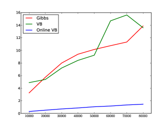
Figure 3. Time used by the algorithms (in hours) given the number of the documents.

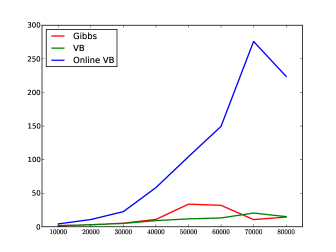
Figure 4. Perplexity on held-out documents as a function of number of documents analyzed.

The fastest algorithm is Online VB, other two have similar time complexity with a large note: VB algorithm converged every time while Gibbs sampling algorithm did not converge. Unexpected, Online VB does not perform as well as other two but in practice still gives reasonably goodExplain unexpected results. Our future goal is to explain the results obtained by experiments.

We see that Gibbs sampling and VB are similar with respect to performance. But if Gibbs sampling converged, we would expect its better performance.

Therefore we recommend Online VB algorithm for practical use, if time is a factor.

5. ACKNOWLEDGMENT

The authors gratefully acknowledge that the funding for this work was provided by the project XLIKE (ICT-
257790-STREP).

References

- [1] David M. Blei, Andrew Y. Ng, and Michael I. Jordan. Latent dirichlet allocation. J. Mach. Learn. Res., 3:993–1022, March 2003.
- [2] Wim De Smet and Marie-Francine Moens. Cross-language linking of news stories on the web using interlingual topic modelling. In Proceedings of the 2nd ACM workshop on Social web search and mining, SWSM ’09, pages 57–64, New York, NY, USA, 2009. ACM.
- [3] A. P. Dempster, N. M. Laird, and D. B. Rubin. Maximum likelihood from incomplete data via the em algorithm. JOURNAL OF THE ROYAL STATISTICAL SOCIETY, SERIES B, 39(1):1–38, 1977.
- [4] Gregor Heinrich. Parameter estimation for text analysis. Technical report, Fraunhofer IGD, Darmstadt, Germany, 2005.
- [5] Matthew D. Hoffman, David M. Blei, and Francis R. Bach. Online learning for latent dirichlet allocation. In NIPS, pages 856–864. Curran Associates, Inc., 2010.
- [6] Michael I. Jordan, Zoubin Ghahramani, Tommi S. Jaakkola, and Lawrence K. Saul. An introduction to variational methods for graphical models. Mach. Learn., 37(2):183–233, November 1999.