Delayed feedback control of self-mobile cavity solitons

Abstract

Control of the motion of cavity solitons is one the central problems in nonlinear optical pattern formation. We report on the impact of the phase of the time-delayed optical feedback and carrier lifetime on the self-mobility of localized structures of light in broad area semiconductor cavities. We show both analytically and numerically that the feedback phase strongly affects the drift instability threshold as well as the velocity of cavity soliton motion above this threshold. In addition we demonstrate that non-instantaneous carrier response in the semiconductor medium is responsible for the increase in critical feedback rate corresponding to the drift instability.

The emergence of spatial-temporal dissipative structures far from equilibrium is a well documented issue since the seminal works of Turing Turing , Prigogine, and Lefever Prigogine1 . Dissipative structures have been theoretically predicted and experimentally observed in numerous nonlinear chemical, biological, hydrodynamical, and optical systems (for reviews on this issue see Review1 ; Review2 ). They can be periodic or localized in space Barland . Localized structures of light in nonlinear laser systems often called cavity solitons are among the most interesting spatiotemporal patterns occurring in extended nonlinear systems. They have attracted growing interest in optics due to potential applications for all-optical control of light, optical storage, and information processing Barland .

Localized structures may loose their stability and start to move spontaneously as a result of symmetry breaking drift bifurcation due to finite relaxation time TSB93 -Gurevich or delayed feedback Tlidi1 -Gurevich13 . The motion of cavity soliton can also be triggered by an external symmetry breaking effects such as a phase gradient Turaev08 , a symmetry breaking due to off-axis feedback Ramazza2 , or resonator detuning Kestas , and an Ising-Bloch transition Coullet ; Michaelis ; Staliunas .

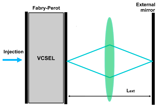
Figure 1: Schematic setup of a nonlinear Fabry-Perot cavity based on a vertical-cavity surface emitting laser (VCSEL) structure, driven by a coherent externally injected beam. The cavity is subject to delayed self-imaging optical feedback from an external mirror located at a distance $L_{ext}$ from the VCSEL output facet.

In what follows we investigate a drift instability of the cavity solitons induced by the time-delayed feedback, which provides a robust and a controllable mechanism, responsible for the appearance of a spontaneous motion. Moving localized strutures and fronts were predicted to appear in extended nonlinear optical  Tlidi1 -Gurevich13 and population dynamics ecology systems, as well as in several chemical and biological systems, described by reaction-diffusion models reaction-diffusion . Previous works revealed that when the product of the delay time and the rate of the feedback exceeds some threshold value, cavity solitons start to move in an arbitrary direction in the transverse plane Tlidi1 -Gurevich13 . In these studies, the analysis was restricted to the specific case of nascent optical bistability described by the real Swift-Hohenberg equation with a real feedback term.

The purpose of the present Letter is to study the role of the phase of the delayed feedback and the carrier lifetime on the motion of cavity solitons in broad-area semiconductor cavities. This simple and robust device received special attention owing to advances in semiconductor technology. We show that for certain values of the feedback phase cavity soliton can be destabilized via a drift bifurcation leading to a spontaneous motion in the transverse direction. Furthermore, we demonstrate that the slower is the carrier decay rate in the semiconductor medium, the higher is the threshold associated with the motion of cavity solitons. Our analysis has obviously a much broader scope than semiconductor cavities and could be applicable to large variety of optical and other systems.

We consider a broad-area semiconductor cavity operating below the lasing threshold and subject to a coherent optical injection and an optical feedback from a distant mirror in a self-imaging configuration, see Fig. 1. The time-delayed feedback is modeled according to Rosanov-Lang-Kobayashi-Pyragas approach rosanov75 . This device can be described by the following dimensionless equations KM1 ; KM2

$$\frac{dE}{dt} = -\left(\mu+i\theta\right)E+2C(1-i\alpha)(N-1)E$$

$$+ E_{i}+\eta e^{i\varphi}[E(t)-E(t-\tau)]+i\nabla^{2}E\,,$$

$$\frac{dN}{dt} = -\gamma\left[N-I+(N-1)\left|E\right|^{2}-d\nabla^{2}N\right]\,,$$ (2)

where $E$ is the slowly varying electric field envelope and $N$ is the carrier density. The parameter $\alpha$ describes the linewidth enhancement factor, $\mu={\tilde{\mu}+\eta\cos{\varphi}}$, and $\theta={\tilde{\theta}}+\eta\sin{\varphi}$, where ${\tilde{\mu}}$ and ${\tilde{\theta}}$ are the cavity decay rate and the cavity detuning parameter, respectively. Below we will assume $\eta$ to be small enough, so that we can neglect the dependence of the parameters $\mu$ and $\theta$ on $\phi$. The parameter $E_{i}$ is the amplitude of the injected field, $C$ is the bistability parameter, $\gamma$ is the carrier decay rate, $I$ is the injection current, and $d$ is the carrier diffusion coefficient. The diffraction of light and the diffusion of the carrier density are described by the terms $i\nabla^{2}E$ and $d\nabla^{2}N$, respectively, where $\nabla^{2}$ is the Laplace operator acting in the transverse plane $(x,\,y)$. The feedback is characterized by the delay time $\tau=2L_{ext}/c$, the feedback rate $\eta\geq 0$, and phase $\varphi$, where $L_{ext}$ is the external cavity length, and $c$ is the speed of light.

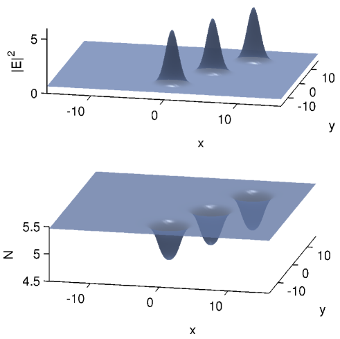
Figure 2: Field intensity (top) and carrier density $N$ (bottom) of two-dimensional moving cavity soliton at different times. The laser parameters are $C=0.45$, $\theta=-2$, $\alpha=5$, $\gamma=0.05$, $d=0.052$, $\mu=2$. The injection is $E_{i}=0.8$, and the feedback parameters are $\tau=200$, $\eta=0.07$, and $\varphi=3.5$. Split-step Fourier method was used to obtain solitons at $t=28000$, $t=30000$, and $t=32000$ (from right to left).

In the absence of delayed feedback, $\eta=0$, we recover the mean field model Spinelli_pra98 , which supports stable stationary patterns and localized structures SC-semiC . In the case of one spatial dimension the localized solutions correspond to homoclinic solutions of Eqs. (Delayed feedback control of self-mobile cavity solitons) and (2) with $\frac{dE}{dt}=\frac{dN}{dt}=0$ and the transverse coordinate $x$ considered as a time variable. They are generated in the subcritical domain, where a uniform intensity background and a branch of spatially periodic pattern are both linearly stable Barland . When the feedback rate $\eta$ exceeds a certain critical value, a cavity soliton can start to move, see Fig. 2. Since the system is isotropic in the $(x,y)$-transverse plane, the velocity of the moving soliton has an arbitrary direction. Numerical simulations were performed using the split-step Fourier method with periodic boundary conditions in both transverse directions.

To calculate the critical value of the feedback rate, which corresponds to the drift instability threshold, and small cavity soliton velocity $v=|{\mathbf{v}}|$ near this threshold, we look for a solution of Eqs. (Delayed feedback control of self-mobile cavity solitons) and (2) in the form of a slowly moving cavity soliton expanded in power series of $v$: $E=E_{0}(\boldsymbol{\xi})+v\,\left[E_{1}(\boldsymbol{\xi})+vE_{2}(\boldsymbol{\xi})+v^{2}E_{3}(\boldsymbol{\xi})+...\right]$ and $N=N_{0}(\boldsymbol{\xi})+v\,\left[N_{1}(\boldsymbol{\xi})+vN_{2}(\boldsymbol{\xi})+v^{2}N_{3}(\boldsymbol{\xi})+...\right]$. Here $E=E_{0}(\mathbf{r})$ and $N=N_{0}(\mathbf{r})$ is the stationary soliton profile, $\boldsymbol{\xi}=\mathbf{r}-v\,\mathbf{e}\,t$, $\mathbf{r}=(x,\,y)$, and $\mathbf{e}$ is the unit vector in the direction of the soliton motion. Substituting this expansion into Eqs. (1) and (2) and collecting the first order terms in small parameter $v$ we obtain:

$$L\left(\begin{array}[]{l}\operatorname{Re}E_{1}\\ \operatorname{Im}E_{1}\\ N_{1}\end{array}\right)=\left(\begin{array}[]{l}\operatorname{Re}(w_{01}-\eta\tau w_{01}e^{i\varphi})\\ \operatorname{Im}(w_{01}-\eta\tau w_{01}e^{i\varphi})\\ \gamma^{-1}m_{01}\end{array}\right)$$ (9)

with $w_{01}={\mathbf{e}}\cdot\nabla E_{0}$ and $m_{01}={\mathbf{e}}\cdot\nabla N_{0}$. The linear operator $L$ is given by

$$L=\left(\begin{array}[]{ccc}\mu-2Cn_{0}&\nabla_{eff}^{2}&-2C(A_{0}+\alpha B_{0})\\ -\nabla_{eff}^{2}&\mu-2Cn_{0}&-2C(B_{0}-\alpha A_{0})\\ 2n_{0}A_{0}&2n_{0}B_{0}&-d\nabla^{2}+1+|E_{0}|^{2}\end{array}\right),$$

where $A_{0}=\operatorname{Re}E_{0}$, $B_{0}=\operatorname{Im}E_{0}$, $\nabla_{eff}^{2}=\nabla^{2}-\theta-2C\,\alpha\,n_{0}$, and $n_{0}=N_{0}-1$. By applying the solvability condition to the right hand side of Eq. (3), we obtain the drift instability threshold

$$\eta=\eta_{0}=\frac{1}{\tau}\frac{1+\gamma^{-1}b}{\sqrt{1+a^{2}}\cos(\varphi+\arctan{a})}$$ (10)

with $a=(\langle\operatorname{Re}w_{01},Y\rangle-\langle\operatorname{Im}w_{01},X\rangle)/g$, $b=\langle m_{01},Z\rangle/g$, and $g=\langle\operatorname{Re}w_{01},\,X\rangle+\langle\operatorname{Im}w_{01},\,Y\rangle$. Here, the eigenfunction ${\psi}^{\dagger}=\left(X,\,Y,\,Z\right)^{T}$ is the solution of the homogeneous adjoint problem $L^{\dagger}\psi^{\dagger}=0$ and the scalar product $\langle\cdot\rangle$ is defined as $\langle\psi_{1},\,\psi_{2}\rangle=\int_{-\infty}^{+\infty}\psi_{1}\psi_{2}^{\dagger}\,d{\mathbf{r}}$. To estimate the coefficients $a$ and $b$ we have calculated the function $\psi$ numerically using the relaxation method in two transverse dimensions, $(x,y)$.

It is noteworthy that since the stationary soliton solution does not depend on the carrier relaxation rate $\gamma$, the coefficients $a$ and $b$ in the threshold condition (10) are also independent of $\gamma$. In the limit of instantaneous carrier response, $\gamma\rightarrow\infty$, and zero feedback phase, $\varphi=0$, we recover from (10) the threshold condition obtained earlier for the drift instability of cavity solitons in the Swift-Hohenberg equation with delayed feedback, $\eta_{0}=\tau^{-1}$Tlidi1 . Note that the drift instability exists in Eqs. (Delayed feedback control of self-mobile cavity solitons) and (2) only for those feedback phases when the cosine function is positive in the denominator of Eq. (10). Furthermore, at $\gamma\to\infty$, $a\neq 0$, and $\varphi=-\arctan{a}$ the critical feedback rate appears to be smaller than that obtained for the real Swift-Hohenberg equation, $\eta_{0}=\tau^{-1}/\sqrt{1+a^{2}}<\tau^{-1}$.

In order to calculate the first order corrections $E_{1}$ and $N_{1}$ to the stationary soliton solution $E_{0}$ and $N_{0}$ we have solved the system (9) numerically using the relaxation method. The second order corrections $E_{2}$ and $N_{2}$ have been obtained in a similar way by equating the second order terms in the small parameter $v$. Finally, assuming that a small deviation of the feedback rate from the drift bifurcation point (10) is of the order $v^{2}$ and equating the third order terms in $v$, we obtain

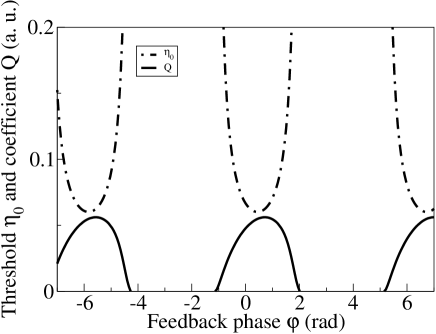
Figure 3: Threshold $\eta_{0}$ associated with the moving cavity soliton (dash-dotted line) given by Eq. (10) and coefficient $Q$ in the expression for the soliton velocity (12) calculated numerically using Eq. (13) (solid line). The parameters are $\mu=1$, $\theta=-2$, $C=0.45$, $\alpha=5$, $\gamma=0.05$, $\tau=200$, $d=0.052$, $E_{i}=0.8$, $I=2$.

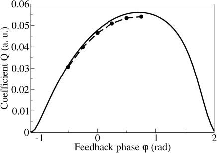
Figure 4: Coefficient $Q$ in the expression for the soliton velocity (12) calculated numerically as a function of the phase $\varphi$ of the delayed feedback (solid line). The circles indicate the values of $Q$ estimated by direct numerical integration of Eqs. (Delayed feedback control of self-mobile cavity solitons) and (2) using the split-step Fourier method. Parameters are the same as in Fig. 3.

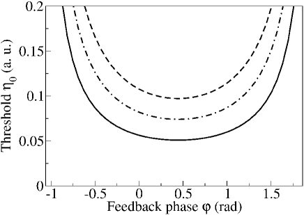
Figure 5: Threshold associated with the motion of cavity soliton as a function of the phase of delayed feedback obtained for different values of the carrier decay rate: $\gamma=0.06$ (solid), $\gamma=0.04$ (dash-dotted), $\gamma=0.03$ (dashed). Other parameters are the same as in Fig. 3.

$$v^{2}L\begin{pmatrix}\operatorname{Re}E_{3}\\ \operatorname{Im}E_{3}\\ N_{3}\end{pmatrix}=\begin{pmatrix}\operatorname{Re}[-r_{1}+v^{2}(\eta_{0}\tau e^{i\varphi}W_{\tau}+r_{3})]\\ \operatorname{Im}[-r_{1}+v^{2}(\eta_{0}\tau e^{i\varphi}W_{\tau}+r_{3})]\\ v^{2}(\gamma^{-1}m_{21}+r_{n})\end{pmatrix},\,$$ (11)

$$r_{1} = (\eta-\eta_{0})e^{i\varphi}\tau w_{01},$$

$$W_{\tau} = \tau^{2}w_{03}/6+\tau w_{12}/2+w_{21},$$

$$r_{3} = w_{21}+2C(1-i\alpha)(N_{1}E_{2}+N_{2}E_{1}),$$

$$r_{n} = -N_{1}|E_{1}|^{2}-N_{2}(E_{0}^{*}E_{1}+E_{0}E_{1}^{*})-$$

$$- N_{1}(E_{0}^{*}E_{2}+E_{0}E_{2}^{*})-n_{0}(E_{1}E_{2}^{*}+E_{2}E_{1}^{*})\,,$$

where $w_{03}={\mathbf{e}}\cdot\nabla({\mathbf{e}}\cdot\nabla({\mathbf{e}}\cdot\nabla E_{0}))$, $w_{12}={\mathbf{e}}\cdot\nabla({\mathbf{e}}\cdot\nabla E_{1})$, $w_{21}={\mathbf{e}}\cdot\nabla E_{2}$, and $m_{21}={\mathbf{e}}\cdot\nabla N_{2}$. The solvability condition for Eq. (11) requires orthogonality of the right hand side of this equation to the eigenfunction $\psi^{\dagger}$ of the adjoint linear operator $L^{\dagger}$. This condition yields the following expression for the soliton velocity:

$$v = (\eta-\eta_{0})^{1/2}Q,$$ (12)

$$Q^{2} = \frac{\tau\,g\sqrt{1+a^{2}}\cos{(\varphi+\arctan{a})}}{\eta_{0}\,\tau h_{\tau}\sqrt{1+p_{\tau}^{2}}\cos{(\varphi+\arctan{p_{\tau}})}+q+s/\gamma}\,$$ (13)

with $h_{\tau}=\langle\operatorname{Re}W_{\tau},X\rangle+\langle\operatorname{Im}W_{\tau},Y\rangle$, $p_{\tau}=(\langle\operatorname{Re}W_{\tau},Y\rangle-\langle\operatorname{Im}W_{\tau},X\rangle)/h$, $q=\langle r_{n},Z\rangle$, and $s=\langle m_{21},Z\rangle$. Here, $h_{\tau}=\langle\operatorname{Re}W_{\tau},X\rangle+\langle\operatorname{Im}W_{\tau},Y\rangle$, $p_{\tau}=(\langle\operatorname{Re}W_{\tau},Y\rangle-\langle\operatorname{Im}W_{\tau},X\rangle)/h$, $q=\langle r_{n},Z\rangle$, and $s=\langle m_{21},Z\rangle$. In the case of zero feedback phase and instantaneous carrier response, $\gamma^{-1}=\varphi=0$, the change of the soliton shape induced by its spontaneous motion is of order $v^{3}$ Gurevich13 ($E_{1}=N_{1}=E_{2}=N_{2}=0$), and, hence, we have $q=r_{n}=s=0$ and $W_{\tau}=\tau^{2}w_{03}/6$. Therefore, in this case the expression for the coefficient $Q$ in Eq. (12) is transformed into $Q^{2}=g/(6\tau^{2}h^{\prime})$ with $h^{\prime}=\langle\operatorname{Re}w_{03},X\rangle+\langle\operatorname{Im}w_{03},Y\rangle$, and we recover a result similar to that obtained earlier for the real Swift-Hohenberg equation with delayed feedback Tlidi1 , $v^{2}=(\eta-\eta_{0})g/(6\tau^{2}h^{\prime})$.

The dependence of the critical feedback rate $\eta_{0}$ on the feedback phase $\varphi$, calculated using Eq. (10) is shown in Fig. 3 by the dash-dotted curves. One can see, that the drift instability exists only within the subinterval $(\varphi_{min}-\pi/2,\varphi_{min}+\pi/2)$ of the interval $(\varphi_{min}-\pi,\varphi_{min}+\pi)$, where $\varphi_{min}=-\arctan{a}$ is the feedback phase, corresponding to the lowest critical feedback rate $\eta_{0}^{min}=(1+\gamma^{-1}b)/(\tau\sqrt{1+a^{2}})$. In addition, $\eta_{0}$ increases very rapidly when approaching the boundaries of this subinterval. The solid lines in Fig. 3 illustrate the dependence of the coefficient $Q$, defined by Eq. (13), on the phase $\varphi$. This coefficient determines the growth rate of the soliton velocity with the square root of the deviation of the feedback rate from the drift bifurcation point, $(\eta-\eta_{0})^{1/2}$. Finally, it is seen from Fig. 4 that the values of the coefficient $Q$ obtained from Eq. (13) are in a good agreement with those of the quantity $v(\eta-\eta_{0})^{-1/2}$ estimated by calculating the soliton velocity near the drift instability threshold with the help of direct numerical simulations of the model equations (Delayed feedback control of self-mobile cavity solitons) and (2).

The impact of carrier decay rate $\gamma$ on the soliton drift instability threshold is illustrated in Fig. 5. It is seen that the threshold value of the feedback rate $\eta_{0}$ increases with $\gamma$, which indicates that the coefficient $b$ in Eq. 10 must be positive. Thus, non-instantaneous carrier response in a semiconductor cavity leads to a suppression of the drift instability of cavity solitons.

To conclude, we have shown analytically and verified numerically that the mobility properties of transverse localized structures of light in a broad area semiconductor cavity with delayed feedback are strongly affected by the feedback phase. In particular, the drift instability leading to a spontaneous motion of cavity solitons in the transverse direction can develop with the increase of the feedback rate only in a certain interval of the feedback phases. Furthermore, we have demonstrated that the critical value of feedback rate corresponding to the drift instability threshold is higher in the case of a semiconductor cavity with slow carrier relaxation rate than in the instantaneous nonlinearity case. The results presented here constitute a practical way of controlling the mobility properties of cavity solitons in broad area semiconductor cavities.

A.P. and A.G.V. acknowledge the support from SFB 787 of the DFG. A.G.V. and G.H. acknowledges the support of the EU FP7 ITN PROPHET and E.T.S. Walton Visitors Award of the Science Foundation Ireland. With the support of the F.R.S.-FNRS. This research was supported in part by the Interuniversity Attraction Poles program of the Belgian Science Policy Office under Grant No. IAP P7-35.

References

- (1) A. M. Turing, Philosophical Transactions of the Royal Society of London, 237, 37 (1952).
- (2) I. Prigogine and R. Lefever, J. Chem. Phys. 48, 1695 (1968).
- (3) N. N. Rosanov, Progress in Optics, 35, 1 (1996); V. S. Zykov, Simulation of Wave Processes in Excitable Media (Manchester University, Manchester, UK, 1987); J.D. Murray, Mathematical Biology, 5Springer 2002); N.N. Rosanov, Spatial Hysteresis and Optical Patterns (Springer, Berlin, 2002); A. S. Mikhailov and K. Showalter, Phys. Rep. 425, 79 (2006); L.A Lugiato, Journal of Quantum Electronics, IEEE, 39, 193 (2003). M. Tlidi and P. Mandel, Journal of Optics B: Quantum and Semiclassical Optics, 6, R60 (2004); G. Purwins et al., Adv. Phys. 59, 485 (2010).
- (4) D. Mihalache et al., Prog. Opt. 27, 229 (1989); K. Staliunas and V. J. Sanchez-Morcillo, Transverse Patterns in Nonlinear Optical Resonators, Springer Tracts in Modern Physics (Springer-Verlag, Berlin, 2003); Y.S. Kivshar and G. P. Agrawal, Optical Solitons: From Fiber to Photonic Crystals (Academic, New York, 2003); B. A. Malomed, D. Mihalache, F. Wise, and L. Torner, J. Optics B: Quant. Semicl. Opt. 7, R53-R72 (2005); M. Tlidi et al., Chaos 17, 037101 (2007); N. Akhmediev and A. Ankiewicz, Dissipative Solitons: From Optics to Biology and Medicine (Springer-Verlag, Berlin, Heidelberg, 2008); O. Descalzi, M. Clerc, S. Residori, and G. Assanto, Localized States in Physics: Solitons and Patterns (Springer, New York, 2011); L. Ridol, P. D’Odorico, F. Laio, Noise-induced phenomena in the environmental sciences, (Cambridge University Press, 2011)
- (5) N.N. Rosanov and G.V. Khodova, JOSA B, 7, 1057 (1990); H.R. Brand and R.J. Deissler, Phys. Rev. Lett. 63, 2801 (1989); B. A. Malomed, Phys. Rev. A 44, 6954 (1991); B. A. Malomed, Phys. Rev. E 58, 7928 (1998); M. Tlidi, P. Mandel, and R. Lefever, Phys. Rev. Lett. 73, 640 (1994); A. J. Scroggie et al., Chaos Solitons Fractals 4, 1323 (1994); G. Slekys, K. Staliunas, and C. O. Weiss, Opt. Commun. 149, 113 (1998); S. Barland et al., Nature 419, 699 (2002); X. Hachair, G. Tissoni, H. Thienpont, and K. Panajotov, Phys. Rev. A 79, 011801(R) (2009) A.G. Vladimirov, R. Lefever, and M. Tlidi, Phys.Rev. A 84, 043848 (2011).
- (6) C.O. Weiss, H.R.Telle, K. Staliunas, and M. Brambilla, Phys. Rev. A 47, R1616 (1993).
- (7) S.V. Fedorov, A.G. Vladimirov, G.V. Khodova, and N.N. Rosanov, Phys. Rev. E 61, 5814 (2000).
- (8) S.V. Gurevich, H.U. Bödeker, A.S. Moskalenko, A.W. Liehr, and H.-G. Purwins, Physica D 199, 115 (2004).
- (9) M. Tlidi, A.G. Vladimirov, D. Pieroux, and D. Turaev, Phys. Rev. Lett. 103, 103904 (2009);
- (10) K. Panajotov and M. Tlidi, Eur. Phys. J. D 59, 67 (2010).
- (11) M. Tlidi, E. Averlant, A. Vladimirov, and K. Panajotov, Phys. Rev. A 86, 033822 (2012).
- (12) S. V. Gurevich and R. Friedrich, Phys. Rev. Lett. 110, 014101 (2013).
- (13) D. Turaev, M. Radziunas, and A.G. Vladimirov, Phys. Rev. E 77, 065201(R) (2008).
- (14) P. Coullet, J. Lega, B. Houchmanzadeh, and J. Lajzerowicz, Phys. Rev. Lett. 65, 1352 (1990).
- (15) D. Michaelis, U. Peschel, F. Lederer, D.V. Skryabin, and W.J. Firth, Phys. Rev. E 63, 066602 (2001).
- (16) K. Staliunas and V.J. Sanchez-Morcillo, Phys. Rev. E 72, 016203 (2005).
- (17) P.L. Ramazza, S. Ducci, and F.T. Arecchi, Phys. Rev. Lett. 81, 4128 (1998); R. Zambrini and F. Papoff, Phys. Rev. Lett. 99, 063907 (2007); S. Coen et al., Phys. Rev. Lett. 83, 2328 (1999).
- (18) K. Staliunas and V.J. Sanchez-Morcillo, Phys. Rev. A 57, 1454 (1998).
- (19) V. Ortega-Cejas, J. Fort, and V. Méndez, Ecology, 85, 258 (2004).
- (20) S. Coombes and C. R. Laing, Physica D 238, 264 (2009); M.A. Dahlem, F. M. Schneider, and E. Schöll, Chaos, 18, 026110 (2008); F.M. Schneider, M.A. Dahlem, and E. Schöll, Chaos 19, 015110 (2009); M.A. Dahlem et al., Physica D 239, 889 (2010); D.A. Jones, H. L. Smith, H.R. Thieme, and G. Röst, SIAM J. Appl. Math., 72, 670 (2012); M. Tlidi, A. Sonnino, and G. Sonnino, Phys. Rev. E 87, 042918 (2013); S. V. Gurevich, Phys. Rev. E 87, 052922 (2013).
- (21) N.N. Rosanov, Sov. J. Quantum Electronics, vol. 4(10), 1191 (1975); R. Lang and K. Kobayashi, IEEE Quantum Electron. 16, 347 (1980); K. Pyragas, Phys. Lett. A 170, 421 (1992).
- (22) L. Spinelli, G. Tissoni, M. Brambilla, F. Prati, L. A. Lugiato, Phys. Rev. A 58, 2542 (1998).
- (23) X. Hachair, S. Barland, L. Furfaro, M. Giudici, S. Balle, J.R. Tredicce, M. Brambilla, T. Maggipinto, I.M. Perrini, G. Tissoni, and L. Lugiato, Phys. Rev. A 69, 043817 (2004).