One cannot hear the density of a drum
(and further aspects of isospectrality)

Abstract

It is well known that certain pairs of planar domains have the same spectra of the Laplacian operator. We prove that these domains are still isospectral for a wider class of physical problems, including the cases of heterogeneous drums and of quantum billiards in an external field. In particular we show that the isospectrality is preserved when the density or the potential are symmetric under reflections along the folding lines of the domain. These results are also confirmed numerically using the finite difference method: we find that the pairs of numerical matrices obtained in the discretization are exactly isospectral up to machine precision.

In an important and influential paper, Kac proposed an interesting problem, summarized in the title of the paper itself: ”can one hear the shape of a drum?” Kac66 . From a mathematical point of view, the spectrum of a drum corresponds to the set of eigenvalues of the negative Laplacian on a given planar domain, where the solutions vanish at the border (Dirichlet boundary conditions). Therefore, Kac’s question can be rephrased as ”are there nonisometric planar domains where the Laplacian has the same spectrum?”. A partial answer to the question comes from Weyl’s law: although in most cases, one does not know the spectrum of a given domain exactly, the asymptotic behavior of the eigenvalues is related to the geometrical properties of the domain (area, perimeter, …). As a result it is possible to distinguish drums with different area and perimeter just by hearing their sound. This result however does not exclude the existence of nonisometric isospectral domains of equal area and perimeter.

In 1992, twenty five years after the publication of Ref. Kac66 , Gordon, Webb and Wolpert GWW92 ; GWW92b found a first example of a pair of nonisometric planar domains with the same Laplace spectrum (see Fig. 1) using a theorem by Sunada Sunada85 . Bérard has given a simple proof of the isospectrality constructing a map which takes an eigenfunction in one domain and maps it into an eigenfunction of the second domain Berard92 ; Berard93 . Buser et al. Buser94 have used this ”transplantation” approach to obtain a large number of isospectral planar domains, while Chapman has visualized this result in terms of ”paper–folding” Chap95 . A discussion of the transplantation method is also found in Okada01 . Isospectral domains with fractal border have been studied by Sleeman and Hua Sleeman00 .

The isospectrality of these domains has later been verified both numerically WSM95 ; Driscoll97 and experimentally using microwave cavities SK94 ; Even99 ; Dhar03 .

More recently, isospectral electronic nanostructures of shapes similar to those of Fig. 1 have been built by Moon et al Moon08 . The extra degree of freedom provided by the isospectrality has been used to extract the quantum phase of the electron wave functions. The reader interested in a detailed account of the present state of the research in this area should refer to the recent review by Giraud and Thas GT10 .

In this paper we want to show that it is possible to generalize the results of Ref. GWW92 ; GWW92b ; Berard92 ; Berard93 to a wider class of physical problems, such as the case of heterogeneous drums or of quantum billiards in an external field. We will prove that, under certain conditions, the pairs of isospectral domains of the Laplacian remain isospectral even in these cases. These results may be summarized saying that one cannot hear the shape of an inhomogeneous drum, nor distinguish two quantum billiards in an external field uniquely by their spectrum.

A related but different problem has been studied by Gottlieb Gottlieb04 ; Gottlieb06 and by Knowles and McCarthy KMC04 , who have found examples of materially isospectral congruent membranes, i.e. isospectral membranes with the same shape but different densities. In particular, the authors of KMC04 have used a conformal transformation on the domains of Fig. 1, obtaining a pair of inhomogeneous isospectral membranes of circular shape. Holmgren et al. Capi06 have analysed the problem of hearing the composition of an inhomogeneous drum using tools of asymptotic linear algebra on the associated numerical problem.

Isospectrality— Bérard has proved that it is possible to map an eigenfunction of one of the domains of Fig. 1 into an eigenfunction of the other domain. Both domains in the figure are made of seven building blocks, which are triangles of angles $(45^{0},45^{0},90^{0})$. The triangles of the first domain are labeled as shown in the figure.

Assuming that an eigenfunction of the first domain is known, the linear combinations shown in the second domain of Fig. 1 are also solutions of the Laplacian in each triangle. Here the notation $\bar{A}$ means that the solution in $A$ is reflected with respect to the dashed line. It is easy to see that the function obtained with these linear combinations and its gradient are everywhere continuous inside the domain and that it vanishes at the border. Therefore this function is an eigenfunction of the second domain with the same eigenvalue.

It is important to notice that the building blocks may be classified into two classes, where the blocks belonging to the same class are related by an even number of reflections along the dashed lines: $\left\{A,C,E\right\}$ and $\left\{B,D,F,G\right\}$. For instance, if we consider the first domain in the figure and we set the origin in the upper vertex of the triangle A, we see that a function $f(x,y)$ defined on A transforms under reflection along the dashed line into a function $f(y,x)$ on B; a further reflection along the horizontal dashed line, transforms this function into $f(y,-x)$, which can be obtained from the first one with a simple rotation.

One may generate each of the two isospectral domains of Fig. 1 starting with a single building block with repeated reflections along the dashed lines. Notice that the linear combinations in the second domain of Fig. 1 only mix functions belonging to the same class (observe that under reflection a function changes class).

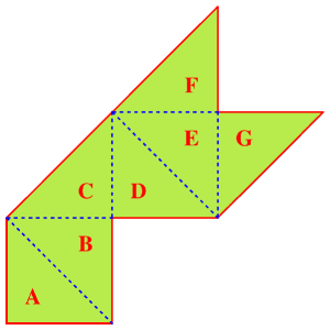
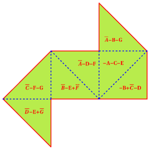
Figure 1: (color online) GWW isospectral drums.

Consider now the eigenvalue equation

$$\hat{H}\psi_{n}=E_{n}\psi_{n}$$

over the first domain of Fig. 1. Here $\hat{H}$ is a Hermitian operator, which contains the Laplacian and with an explicit dependence on the coordinates. We assume that we know an eigenfunction of $\hat{H}$ and we want to see under what conditions the linear combinations in the second domain of Fig. 1 provide an eigenfunction of $\hat{H}$.

In the case of a homogeneous drum, the reflection of the eigenfunction along a dashed line is still an eigenfunction of the Laplacian, since this operator commutes with the reflections; in the present case, however, because of the explicit dependence on the coordinates, the operator does not commute with the reflection and therefore the reflection of the function on $A$, $\bar{A}$, is not in general an eigenfunction of $\hat{H}$. However, this problem is solved if the operator $\hat{H}$ in each building block is also obtained from the operators in the neighboring blocks through a reflection along the dashed line separating the two blocks.

In this way, the linear combinations appearing in the second domain Fig. 1 are once again eigenfunctions of the operator; since the function obtained with these linear combinations and its gradient are everywhere continuous in the domain and the function vanishes on the border, it is an eigenfunction of $\hat{H}$ over the second domain. Therefore, the domains are isospectral.

It is useful to discuss two physical examples of isospectral problems of this kind. We consider first the case of an inhomogeneous drum: its vibrations are described by the eigensolutions of the Helmholtz equation

$$\left(-\Delta\right)\psi_{n}(x,y)=E_{n}\Sigma(x,y)\psi_{n}(x,y)$$ (1)

where $\Sigma(x,y)>0$ is the density of the membrane, $(x,y)\in\Omega$, a domain in the plane (we also assume Dirichlet boundary conditions on the border, $\partial\Omega$, $\psi_{n}(x,y)|_{\partial{\Omega}}=0$). It is convenient to convert Eq.(1) to

$$\left[\frac{1}{\sqrt{\Sigma}}\left(-\Delta\right)\frac{1}{\sqrt{\Sigma}}\right]\phi_{n}(x,y)=E_{n}\phi_{n}(x,y)$$ (2)

where $\hat{H}\equiv\frac{1}{\sqrt{\Sigma}}\left(-\Delta\right)\frac{1}{\sqrt{\Sigma}}$ is a Hermitian operator and $\phi_{n}(x,y)\equiv\sqrt{\Sigma}\psi_{n}(x,y)$ Amore10b (notice that Eqs.(1) and (2) have the same spectrum).

According to our previous discussion, the two domains will be isospectral if the density $\Sigma$ in any of the building blocks that compose the domains is the reflection of the density on a neighbouring block along the dashed line separating the two. Notice that the two heterogeneous domains have clearly the same mass (we call $\Omega_{A}$ and $\Omega_{B}$ the domains on the left and the right of Fig.2 respectively and $\Sigma_{A}$ and $\Sigma_{B}$ their densities) $M=\int_{\Omega_{A}}dxdy\ \Sigma_{A}(x,y)=\int_{\Omega_{B}}dxdy\ \Sigma_{B}(x,y)$ and therefore their spectrum has the same asymptotic behavior, provided by Weyl’s law, $E_{n}=4\pi n/M$ ($n\rightarrow\infty$) Amore10a .

Fig. 2 displays a pair of inhomogeneous isospectral drums with a piecewise constant density (the lighter and darker colors in the figures correspond to two different densities $\Sigma_{1}$ and $\Sigma_{2}$). More elaborate examples, with a continuously varying density inside a given block can be easily obtained. Also, one could consider more general shapes of the domains, as those discussed in Buser94 ; Chap95 ; Sleeman00 .

Figure 2: (color online) Inhomogeneous isospectral drums. The regions with larger density are darker.

As a second example of isospectral problem we consider a quantum particle confined in a finite region under the action of an external force (in absence of a force, the operator reduces to the Laplacian, for which the isospectrality has already been proved). Therefore we are interested in the spectrum of the single particle Hamiltonian $\hat{H}=\left[-\frac{\hbar^{2}}{2m}\Delta+V(x,y)\right]$ on each of the two domains of Fig. 1.

In this case the condition of isospectrality requires the potential $V(x,y)$ in each block to be the reflection of the potential on a neighboring block, along the dashed line separating the two. For instance $V(x,y)$ could be the potential generated by the interaction of an electron confined in any of the two domains of Fig. 1 with $7$ pointlike charges $q$ located at the center of mass of each building block. In Fig. 3 we display a simpler example of isospectral quantum billiard: the vector lines represent an electric field of constant magnitude $\mathcal{E}$ pointing in a given direction. Reversing the sign of $\mathcal{E}$ clearly corresponds to inverting the directions of the vectors in the figure.

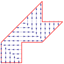
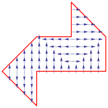
Figure 3: (color online) Isospectral quantum billiards in an electric field. The arrows indicate the direction of the constant electric field.

Numerical experiments— It was noted by Wu, Sprung and Martorell in Ref. WSM95 that the finite difference method provides matrices which are exactly isospectral up to machine precision when applied to the calculation of the spectrum of the Laplacian over the two domains of Fig. 1 (clearly, the same grid size is used in both cases).

We have followed the same strategy of Ref. WSM95 for the general problems discussed in this paper, working with very fine grids (the maximum grid that we have generated contains $200521$ points) and using a collocation approach based on tent functions, which is equivalent to a finite difference approach.

In all our calculations we have found that the matrices obtained in the discretization of the problem are always exactly isospectral, up to machine precision  and therefore we will always report a single numerical value for both domains. This result provides a numerical confirmation of our previous results.

Table 1: Lowest $10$ eigenvalues of the inhomogeneous drums of Fig. 2. Here $\Sigma_{1}=1$ and $\Sigma_{2}=2$.

n	$E_{n}^{\rm(FD)}$	$E_{n}^{\rm(EX)}$
1	1.52189	1.51992
2	2.63494	2.63002
3	3.08334	3.07902
4	4.58312	4.57697
5	4.83882	4.83108
6	6.23355	6.22662
7	6.68975	6.67769
8	7.71814	7.70122
9	7.92551	7.91504
10	8.66913	8.65750

The first example that we have studied is the inhomogeneous drum of Fig. 2 with densities $\Sigma_{1}=1$ (lighther region) and $\Sigma_{2}=2$ (darker region). In Table 1 we report the lowest $10$ eigenvalues of these domains (the building blocks are triangles with angles $45^{0}$, $45^{0}$ and $90^{0}$ and shorter side of length $\ell=2$): the second column contains the results obtained with finite difference with a grid containing $200521$ points; the third column contains the results obtained using Richardson extrapolation on a sequence of approximations obtained using grids with spacing $h=1/4k$, with $k=19,\dots,30$. For all the cases examined this sequence has a monotonical behavior with decreasing $h$ and therefore the extrapolation improves significantly the accuracy of the results. In the case of a homogeneous membrane, where the very precise results of Ref. Driscoll97 are available, this procedure applied on the sequence of eigenvalues obtained with the same grids used here allows one to obtain about four decimal correct for the lowest eigenvalues. We expect roughly the same accuracy here.

The second example that we consider is plotted in Fig.3: in each building block an electric field of constant magnitude points at a given direction. Our numerical results have been obtained setting $\hbar^{2}/2m=1$ and $e=1$, and considering an electric field $\mathcal{E}=5$. The wave functions for the ground state of this problem in the two domains are plotted in Fig. 4. The corresponding eigenvalue obtained using the largest grid ($200521$ points) is $E^{(FD)}_{1}=-1.21302$; the value obtained with extrapolation (see the discussion for the previous example) is $E^{(EX)}_{1}=-1.21311$.

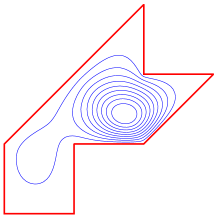
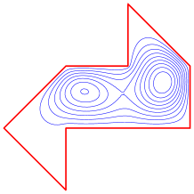
Figure 4: (color online) Wave functions of the ground state of the isospectral Hamiltonians corresponding to Fig.3 with $\mathcal{E}=5$.

In conclusion, we have generalized the results of Gordon,Webb and Wolpert GWW92 to a larger class of physical problems, which include the case of inhomogeneous drums or of quantum billiards in an external field. We have proved that the domains found in Ref. GWW92 are still isospectral when the density or the potential in each building block is obtained from the reflection of the analogous quantities in the neighboring blocks, along the common border separating the two. In particular our results signal the possibility of building isospectral pairs of ”ray-splitting” billiards, i.e. cavities with abrupt changes in the properties of the medium filling it (see the original work by Couchman et al. Ref. Couchman92 and the works by Vaa et al., Ref. Blumel03 ; Blumel05 , containing experimental verification of the theoretical semiclassical formulas).

- (1) M. Kac, Am. Math. Monthly 73, 1 (1966)
- (2) C. Gordon , D. Webb and S. Wolpert, Bull. Am. Math. Soc. 27, 134-138 (1992)
- (3) C. Gordon , D. Webb and S. Wolpert, Invent. Math. 110, 1 (1992)
- (4) T. Sunada, Ann. Math. 121, 248-277 (1985)
- (5) P. Bérard, Math.Ann.292, 547-559 (1992)
- (6) P. Bérard, Journal of the London Mathematical Society 2, 565-576 (1993)
- (7) P. Buser, J. Conway and P. Doyle, Int. Math. Res. Notices 9, 391 (1994)
- (8) S. J . Chapman, Am. Math. Monthly 102, 1 (1995)
- (9) Y. Okada and A. Shudo, J.Phys. A 34, 5911 (2001)
- (10) B.D. Sleeman and C. Hua, Revista Matematica Iberoamericana 16, 351-361 (2000)
- (11) H. Wu, D. W. L. Sprung and J. Martorell, Phys. Rev. E 51, 703-708 (1995)
- (12) T. Driscoll, SIAM Rev. 39, 1 (1997)
- (13) S. Sridhar and A. Kudrolli, Phys. Rev. Lett. 72, 2175 (1994)
- (14) S. Even and P. Pieranski, Europhys. Lett. 47, 531 (1999)
- (15) A. Dhar, D.M. Rao, N. UdayaShankar and S. Sridhar, Phys. Rev. E 68, 026208 (2003)
- (16) C.R. Moon et al., Science 319, 782-787 (2008)
- (17) O. Giraud and K. Thas, Rev. Mod. Phys. 82, 2213-2255 (2010)
- (18) H.P.W. Gottlieb, Inverse Probl. 20, 155 (2004)
- (19) H.P.W. Gottlieb, ANZIAM J. 47, C152-C167 (2006)
- (20) I.W.Knowles and M.L. McCarthy, J. Phys.A 37, 8103 (2004)
- (21) S. Holmgren, S. Serra-Capizzano and P. Sundqvist, Mediterranean Journal of Mathematics 3, 227-249 (2006)
- (22) P. Amore, J.Math.Phys. 51 052105 (2010)
- (23) P. Amore, Europhys. Lett. 92, 10006 (2010)
- (24) L. Couchman, E. Ott and T.M. Antonsen Jr., Phys. Rev. A 46, 6193 (1992)
- (25) C. Vaa, P.M. Koch and R. Blümel, Phys. Rev. Lett. 90, 194102 (2003)
- (26) C. Vaa, P.M. Koch and R. Blümel, Phys. Rev. E 72, 056211 (2005)