Exploratory Learning

Abstract

In multiclass semi-supervised learning (SSL), it is sometimes the case that the number of classes present in the data is not known, and hence no labeled examples are provided for some classes. In this paper we present variants of well-known semi-supervised multiclass learning methods that are robust when the data contains an unknown number of classes. In particular, we present an “exploratory” extension of expectation-maximization (EM) that explores different numbers of classes while learning. “Exploratory” SSL greatly improves performance on three datasets in terms of F1 on the classes with seed examples—i.e., the classes which are expected to be in the data. Our Exploratory EM algorithm also outperforms a SSL method based non-parametric Bayesian clustering.

1 Introduction

In multiclass semi-supervised learning (SSL), it is sometimes the case that the number of classes present in the data is not known. For example, consider the task of classifying noun phrases into a large hierarchical set of categories such as “person”, “organization”, “sports team”, etc., as is done in broad-domain information extraction systems (e.g., [5]). A sufficiently large corpus will certainly contain some unanticipated natural clusters—e.g., kinds of musical scales, or types of dental procedures. Hence, it is unrealistic to assume some examples have been provided for each class: a more plausible assumption is that an unknown number of classes exist in the data, and that labeled examples have been provided for some subset of these classes.

This raises the natural question: how robust are existing SSL methods to unanticipated classes? As we will show experimentally below, SSL methods can perform quite poorly in this setting: the instances of the unanticipated classes might be forced into one or more of the expected classes, leading to a cascade of errors in class parameters, and then to class assignments to other unlabeled examples. To address this problem, we present an “exploratory” extension of expectation-maximization (EM) which explores different numbers of classes while learning.

More precisely, in a traditional SSL task, the learner assumes a fixed set of classes $C_{1},C_{2},\ldots C_{k}$, and the task is to construct a $k$-class classifier using labeled datapoints $X^{l}$ and unlabeled datapoints $X^{u}$, where $X^{l}$ contains a (usually small) set of “seed” examples of each class. In exploratory SSL, we assume the same inputs, but allow the classifier to predict labels from the set $C_{1},\ldots,C_{m}$, where $m\geq{}k$: in other words, every example $x$ may be predicted to be in either a known class $C_{i}\in{C_{1}\ldots C_{k}}$, or an unknown class $C_{i}\in{C_{k+1}\ldots C_{m}}$.

We will show that exploratory SSL can greatly improve performance on noun-phrase classification tasks and document classification tasks, for several well-known SSL methods. E.g. Figure 1 (b) top row shows, the confusion matrices for a traditional SSL method on a 20-class problem at the end of iteration 1 and 15, when the algorithm is presented with seeds for 6 of the classes. Here, red indicates overlap between classes, and dark blue indicates no overlap. So we see that many of the seed classes are getting confused with the unknown classes at the end of 15 iterations of SSL showing semantic drift. With the same inputs, our novel “exploratory” EM algorithm performs quite well (Figure 1 (b) bottom row); i.e. it introduces additional clusters and at the end of 15 iterations improves F1 on classes for which seed examples were provided.

Contributions. We focus on the novel problem of dealing with learning when only fraction of classes are known upfront, and there are unknown classes hidden in the data. We propose a variant of the EM algorithm where new classes can be introduced in each EM iteration. We discuss the connections of this algorithm to the structural EM algorithm. Next we propose two heuristic criteria for predicting when to create new class during an EM iteration, and show that these two criteria work well on three publicly available datasets. Further we evaluate third criterion, that introduces classes uniformly at random and show that our proposed heuristics are more effective than this baseline. Experimentally, Exploratory EM outperforms a semi-supervised variant of non-parametric Bayesian clustering (Gibbs sampling with Chinese Restaurant Process)—a technique which also “explores” different numbers of classes while learning. We also compare our method against a semi-supervised EM method with $m$ extra classes (trying different values of $m$).

In this paper, Exploratory EM is instantiated to produce exploratory versions of three well-known SSL methods: semi-supervised Naive Bayes, seeded K-Means, and a seeded version of EM using a von Mises-Fisher distribution [1]. Our experiments focus on improving accuracy on the classes that do have seed examples—i.e., the classes which are expected to be in the data.

Outline. In Section 2, we first introduce an exploratory version of EM, and then discuss several instantiations of it, based on different models for the classifiers (mixtures of multinomials, K-Means, and mixtures of von Mises-Fisher distributions) and different approaches to introducing new classes. We then compare against an alternative exploratory SSL approach, namely Gibbs sampling with Chinese restaurant process [14]. Section 3 presents experimental results, followed by related work and conclusions.

2 Exploratory SSL Methods

2.1 A Generic Exploratory Learner

Many common approaches to SSL are based on EM. In a typical EM setting, the M-step finds the best parameters $\theta$ to fit the data, $X^{l}\cup X^{u}$, and the E-step probabilistically labels the unknown points with a distribution over the known classes $C_{1},C_{2},\ldots C_{k}$. In some variants of EM, including the ones we consider here, a “hard” assignment is made to classes instead, an approach named classification EM [6]. Our exploratory version of EM differs in that it can introduce new classes ${C_{k+1}\ldots C_{m}}$ during the E-step.

Algorithm 1 EM algorithm for exploratory learning with model selection

1:  function Exploratory EM  ($X^{l}$, $Y^{l}$, $X^{u}$, {$C_{1}\ldots C_{k}$}): $\{C_{k+1}\ldots C_{m}\}$, $\theta^{m}$, $Y^{u}$

2:  Input: $X^{l}$ labeled data points; $Y^{l}$ labels for datapoints $X^{l}$; $X^{u}$ unlabeled datapoints (same feature space as $X^{l}$); {$C_{1}\ldots C_{k}$} set of known classes to which $x$’s belong.

3:  Output: $\{C_{k+1}\ldots C_{m}\}$ newly-discovered classes; $\{\theta^{1},\ldots,\theta^{m}\}$ parameters for all $m$ classes; $Y^{u}$ labels for unlabeled data points $X^{u}$

3:   {Initialize model parameters using labeled data}

4:  $\theta^{1}_{0},\ldots,\theta^{k}_{0}=argmax_{\theta}L(X^{l},Y^{l}|\theta^{k})$

5:  $i$ is # new classes ; $i=0$; CanAddClasses = $true$

6:  while data likelihood not converged AND #classes not converged do

6:     {E step: (Iteration $t$) Make predictions for the unlabeled data-points}

7:    $i_{old}=i$; Compute baseline log-likelihood BaselineLL $=logP(X|\theta^{1}_{t},\ldots,\theta^{k+i_{old}}_{t})$

8:    for $x\in X^{u}$ do

9:       Predict $P(C_{j}|x,\theta^{1}_{t},\ldots,\theta^{k+i}_{t})$ for all labels $1\leq{}j\leq{k+i}$

10:       if nearlyUniform($P(C_{1}|x),\ldots,P(C_{k+i}|x)$) AND CanAddClasses then

11:          Increment $i$; Let $C_{k+i}$ be the new class.

12:          Label $x$ with $C_{k+i}$ in $Y^{u}$, and compute parameters $\theta^{k+i}_{t}$ for the new class.

13:       else

14:          Assign $x$ to $(argmax_{C_{j}}P(C_{j}|x))$ in $Y^{u}$ where $1\leq{}j\leq{k+i}$

15:       end if

16:    end for

17:    $i_{new}=i$; Compute ExploreEM loglikelihood ExploreLL $=logP(X|\theta^{1}_{t},\ldots,\theta^{k+i_{new}}_{t})$

17:     {M step : Recompute model parameters using current assignments for $X^{u}$}

18:    if Penalized data likelihood is better for exploratory model than baseline model then

18:        {Adopt the new model with $k+i_{new}$ classes}

19:       $\theta^{k+i_{new}}_{t+1}=argmax_{\theta}L(X^{l},Y^{l},X^{u},Y^{u}_{t}|\theta^{k+i_{new}})$

20:    else

20:        {Keep the old model with $k+i_{old}$ classes}

21:       $\theta^{k+i_{old}}_{t+1}=argmax_{\theta}L(X^{l},Y^{l},X^{u},Y^{u}_{t}|\theta^{k+i_{old}})$

22:       CanAddClasses = $false$

23:    end if

24:  end while

25:  end function 

Algorithm 1 presents a generic Exploratory EM algorithm (without specifying the model being used). There are two main differences between the algorithm and standard classification-EM approaches to SSL. First, in the E step, each of the unlabeled datapoint $x$ is either assigned to one of the existing classes, or to a newly-created class. We will discuss the “nearUniform” routine below, but the intuition we use is that a new class should be introduced to hold $x$ when the probability of $x$ belonging to existing classes is close to uniform. This suggests that $x$ is not a good fit to any existing classes, and that adding $x$ to any existing class will lower the total data likelihood substantially. Second, in the M-step of iteration $t$, we choose either the model proposed by Exploratory EM method that might have more number of classes than previous iteration $t-1$ or the baseline version with same number of classes as iteration $t-1$. This choice is based on whether exploratory model satisfies a model selection criterion in terms of increased data likelihood and model complexity. If the algorithm decides that baseline model is better than exploratory model in iteration $t$, then from iteration $t+1$ onwards the algorithm won’t introduce any new classes.

2.2 Discussion

Friedman [13] proposed the Structural EM algorithm that combines the standard EM algorithm, which optimizes parameters, with structure search for model selection. This algorithm learns networks based on penalized likelihood scores, in the presence of missing data. In each iteration it evaluates multiple models based on the expected scores of models with missing data, and selects the model with best expected score. This algorithm converges at local maxima for penalized log likelihood (the score includes penalty for increased model complexity).

Similar to Structural EM, in each iteration of Algorithm 1, we evaluate two models, one with and one without adding extra classes. These two models are scored using a model selection criterion like AIC or BIC, and the model with best penalized data likelihood score is selected in each iteration. Further when the model selection criterion fails, the algorithm reverts to standard semi-supervised EM algorithm. Say this model switch happens at iteration $t_{switch}$, then from iteration 1 to $t_{switch}$, Algorithm 1 acts like the structural EM algorithm [13]. From iteration $t_{switch}+1$ till the data likelihood converges, the algorithm acts as semi-supervised EM algorithm.

Next let us discuss the applicability of this algorithm for clustering as well as classification tasks. Notice that Algorithm 1 reverts to an unsupervised clustering method if $X_{l}$ is empty, and reverts to a supervised generative learner if $X_{u}$ is empty. Likewise, if no new classes are generated, then it behaves as a multiclass SSL method; for instance, if the classes are well-separated and $X_{l}$ contains enough labels for every class to approximate these classes, then it is unlikely that the criterion of nearly-uniform class probabilities will be met, and the algorithm reverts to SSL. Henceforth we will use the terms “class” and “cluster” interchangeably.

2.3 Model Selection

For model penalties we tried multiple well known criteria like BIC, AIC and AICc. Burnham and Anderson [4] have experimented with AIC criteria and proposed AICc for datasets where, the number of datapoints is less than 40 times number of features. The formulae for scoring a model using each of the three criteria that we tried are:

$$BIC(g) = -2*L(g)+v*ln(n)$$ (1)

$$AIC(g) = -2*L(g)+2*v$$ (2)

$$AICc(g) = AIC(g)+2*v*(v+1)/(n-v-1)$$ (3)

where $g$ is the model being evaluated, $L(g)$ is the log-likelihood of the data given $g$, $v$ is the number of free parameters of the model and $n$ is the number of data-points.
While comparing two models, a lower value is preferred. The extended Akaike information criterion (AICc) suited best for our experiments since our datasets have large number of features and small number of data points. With AICc criterion, the objective function that Algorithm 1 optimizes is:

$$\max_{\begin{subarray}{c}m,\{\theta^{1}\ldots\theta^{m}\}\end{subarray},m\geq k}\{\text{Log Data Likelihood}-\text{Model penalty}\}$$

$$\text{i.e., }\max_{\begin{subarray}{c}m,\{\theta^{1}\ldots\theta^{m}\},m\geq k\end{subarray}}\{\log P(X|\theta^{1},\ldots,\theta^{m})\}-\{v+(v*(v+1)/(n-v-1))\}$$ (4)

Here, $k$ is the number of seed classes given as input to the algorithm and $m$ is the number of classes in the resultant model ($m\geq k$).

2.4 Exploratory versions of well-known SSL methods

In this section we will consider various SSL techniques, and propose exploratory extensions of these algorithms.

2.4.1 Semi-Supervised Naive Bayes

Nigam et al. [21] proposed an EM-based semi-supervised version of multinomial Naive Bayes. In this model $P(C_{j}|x)\propto P(x|C_{j})*P(C_{j})$, for each unlabeled point $x$. The probability $P(x|C_{j})$ is estimated by treating each feature in $x$ as an independent draw from a class-specific multinomial. In document classification, the features are word occurrences, and the number of outcomes of the multinomial is the vocabulary size.

This method can be naturally used as an instance of Exploratory EM, using the multinomial model to compute $P(C_{j}|x)$ in Line 9. The M step is also trivial, requiring only estimates of $P(w|C_{j})$ for each word/feature $w$.

2.4.2 Seeded K-Means

It has often been observed that K-Means and EM are algorithmically similar. Basu and Mooney [2] proposed a seeded version of K-Means, which is very analogous to Nigam et al’s semi-supervised Naive Bayes, as another technique for semi-supervised learning. Seeded K-Means takes as input a number of clusters, and seed examples for each cluster. The seeds are used to define an initial set of cluster centroids, and then the algorithm iterates between an “E step” (assigning unlabeled points to the closest centroid) and an “M step” (recomputing the centroids).

In the seeded K-Means instance of Exploratory EM, we again define $P(C_{j}|x)\propto P(x|C_{j})*P(C_{j})$, but define $P(x|C_{j})=x\cdot C_{j}$, i.e., the inner product of a vector representing $x$ and a vector representing the centroid of cluster $j$. Specifically, $x$ and $C_{j}$ both are represented as $L_{1}$ normalized TFIDF feature vectors. The centroid of a new cluster is initialized with smoothed counts from $x$. In the “M step”, we recompute the centroids of clusters in the usual way.

2.4.3 Seeded Von-Mises Fisher

The connection between K-Means and EM is explicated by Banerjee et al. [1], who described an EM algorithm that is directly inspired by K-Means and TFIDF-based representations. In particular, they describe generative cluster models based on the von Mises-Fisher (vMF) distribution, which describes data distributed on the unit hypersphere. Here we consider the “hard-EM” algorithm proposed by Banerjee et al, and use it in the seeded (semi-supervised) setting proposed by Basu et al. [2]. This natural extension of Banerjee et al[1]’s work can be easily extended to our exploratory setting.

As in seeded K-Means, the parameters of vMF distribution are initialized using the seed examples for each known cluster. In each iteration, we compute the probability of $C_{j}$ given data point $x$, using vMF distribution, and then assign $x$ to the cluster for which this probability is maximized. The parameters of the vMF distribution for each cluster are then recomputed in the M step. For this method, we use a TFIDF-based $L_{2}$ normalized vectors, which lie on the unit hypersphere.

Seeded vMF and seeded K-Means are closely related—in particular, seeded vMF can be viewed as a more probabilistically principled version of seeded K-Means. Both methods allow use of TFIDF-based representations, which are often preferable to unigram representations for text: for instance, it is well-known that unigram representations often produce very inaccurate probability estimates.

2.5 Strategies for inducing new clusters/classes

Algorithm 2 JS criterion for new class creation

1:  function JSCriterion($[P(C_{1}|x)\ \ldots\ P(C_{k}|x)]$):

2:  Input: $[P(C_{1}|x)\ldots P(C_{k}|x)]$ probability distribution of existing classes for a data point $x$

3:  Output: decision : true iff new class needs to be created

4:  $u$ = [$1/k$ $\ldots$ $1/k$] {i.e., the uniform distribution with current number of classes = $k$}

5:  decision = false

6:  if Jensen-Shannon-Divergence($u$, $P(C_{j}|x)$) $<$ $\frac{1}{k}$ then

7:    decision = true

8:  end if

9:  end function 

Algorithm 3 MinMax  criterion for new class creation

1:  function MinMaxCriterion($[P(C_{1}|x)\ \ldots\ P(C_{k}|x)]$):

2:  Input: $[P(C_{1}|x)\ldots P(C_{k}|x)]$ probability distribution of existing classes for a data point $x$

3:  Output: decision : true iff new class needs to be created

4:  $k$ is the current number of classes

5:  $maxProb$ = max($P(C_{j}|x)$); $minProb$ = min($P(C_{j}|x)$)

6:  if $\frac{maxProb}{minProb}<2$ then

7:    decision = true

8:  end if

9:  end function 

In this section we will formally describe some possible strategies for introducing new classes in the E step of the algorithm. They are presented in detail in Algorithms 2 and 3, and each of these is a possible implementation of the “nearUniform” subroutine of Algorithm 1. As noted above, the intuition is that new classes should be introduced to hold $x$ when the probabilities of $x$ belonging to existing classes are close to uniform. In the JS criterion, we require that Jensen-Shanon divergence between the posterior class distribution for $x$ to the uniform distribution be less than $\frac{1}{k}$. The MinMax criterion is a somewhat simpler approximation to this intuition: a new cluster is introduced if the maximum probability is no more than twice the minimum probability.

2.6 Baseline Methods

Next, we will take a look at various baseline methods that we implemented to measure the effectiveness of our proposed approach.

2.6.1 Random new class creation criterion:

To measure the effectiveness of criteria proposed in Algorithms 2 and 3, we experimented with a random baseline criterion, that returns “true” uniformly at random with probability equal to that of MinMax or JS criterion returning true for the same dataset. This is referred to as Random criterion below.

Algorithm 4 Exploratory Gibbs Sampling with Chinese Restaurant Process

1:  function GibbsCRP ($X^{l}$, $Y^{l}$, $X^{u}$, {$C_{1}\ldots C_{k}$}) : ${C_{k+1}\ldots C_{m}}$, $Y^{u}$

2:  Input: $X^{l}$ labeled data points; $Y^{l}$ labels of $X^{l}$; $X^{u}$ unlabeled data points; {$C_{1}\ldots C_{k}$} set of known classes $x$’s belong to; $P_{new}$ probability of creating a new class.

3:  Output: ${C_{k+1}\ldots C_{m}}$ newly-discovered classes; $Y^{u}$ labels for $X^{u}$

4:  for $x$ in $X^{u}$ do

5:    Save a random class from {$C_{1}\ldots C_{k}$} for $x$ in $Y^{u}$

6:  end for

7:  Set $m=k$

8:  for $t$ : 1 to $numEpochs$ do

9:    for $x_{i}$ in $X^{u}$ do

10:       Let $y_{i}$’s be $x_{i}$’s label in epoch $t-1$

11:       predict $P(C_{j}|x_{i},Y^{l}\cup{}Y^{u}-\{y_{i}\})$    for all labels $1\leq{}j\leq{}m$

12:       $y_{i}^{\prime},m^{\prime}$ = CRPPick($P_{new}$, $P(C_{1}|x_{i}),\ldots,P(C_{m+1}|x_{i})$)

13:       Save $y_{i}^{\prime}$ as $x_{i}$’s label in epoch $t$

14:       $m=m^{\prime}$

15:    end for

16:  end for

17:  end function 

Algorithm 5 Modified CRP criterion for new class creation

1:  function ModCRPPick ($P_{new}$, $P(C_{1}|x),\ldots,P(C_{k+i}|x)$) : $y,i^{\prime}$

2:  Input: $P_{new}$ probability of creating new class; $P(C_{1}|x),\ldots,P(C_{k+i}|x)$ probability of existing classes given $x$

3:  Output: $y$ class for $x$; $i^{\prime}$ new number of classes

4:  $u$ = [$1/{k+i}$ $\ldots$ $1/{k+i}$] {uniform distribution with $k+i$ classes}

5:  $d$ = Jensen-Shannon-Divergence($u$, $P(C_{j}|x)$)

6:  $q$ = $\frac{P_{new}}{((k+i)*d)}$

7:  if a coin with bias $q$ is heads then

7:     {create a new class and assign to that}

8:    $y=k+i+1$ and $i^{\prime}=i+1$

9:  else

9:     {assign to an existing class}

10:    $i^{\prime}=i$ and $y$ = sample from distribution $[P(C_{1}|x)\ \ldots\ P(C_{k}|x)]$

11:  end if

12:  end function 

2.6.2 Semi-supervised EM with $m$ extra classes:

One might argue that the goal of the Exploratory EM algorithm can also be achieved by adding a random number of empty classes to the semi-supervised EM algorithm. We compare our method against the best possible value of this baseline, i.e. by choosing the number of classes that maximizes F1 on the seed classes. Note that in practice, the test labels are not available, so this is the upper bound on performance of this baseline. We compare our method with this upper bound in Section 3. Our method is different from this baseline in two ways. First, it does not need the number of extra clusters as input. Second, it seeds the extra clusters with those datapoints that are unlikely to belong to existing classes, as compared to initializing them randomly.

2.6.3 A seeded Gibbs sampler with CRP:

The Exploratory EM method is broadly similar to non-parametric Bayesian methods, such as the Chinese Restaurant process (CRP) [14]. CRP is often used in non-parametric models (e.g., topic models) that are based on Gibbs sampling, and indeed, since it is straightforward to replace EM with Gibbs-sampling, one can use this approach to estimate the parameters of any of the models considered here (i.e., multinomial Naive Bayes, K-Means, and the von Mises-Fisher distribution). Algorithm 4 presents a seeded version of a Gibbs sampler based on this idea. In brief, Algorithm 4, starts with a classifier trained on the labeled data. Collapsed Gibbs sampling is then performed over the latent labels of unlabeled data, incorporating the CRP into the Gibbs sampling to introduce new classes. (In fact, we use block sampling for these variables, to make the method more similar to the EM variants.)

Note that this algorithm is naturally “exploratory”, in our sense, as it can produce a number of classes larger than the number of classes for which seed labels exist. However, unlike our exploratory EM variants, the introduction of new classes is not driven by examples that are “hard to classify”—i.e., have nearly-uniform posterior probability of membership in existing classes. In CRP method, the probability of creating a new class depends on the data point, but it does not explicitly favor cases where the posterior over existing classes is nearly uniform.

To address this issue, we also implemented a variant of the seeded Gibbs sampler with CRP, in which the examples with nearly-uniform distributions are more likely to be assigned to new classes. This variant is shown in Algorithm 5, which replaces the routine CRPPick in the Gibbs sampler—in brief, we simply scale down the probability of creating a new class by the Jensen-Shannon divergence of the posterior class distribution for $x$ to the uniform distribution. Hence the probability of creating new class explicitly depends on how well the given data point fits in one of the existing classes. An experimental comparison of our proposed method with Gibbs sampling and CRP based baselines is shown in Section 3.2.

3 Experimental Results

We now seek to experimentally answer the questions raised in the introduction. How robust are existing SSL methods, if they are given incorrect information about the number of classes present in the data, and seeds for only some of these classes? Do the exploratory versions of the SSL methods perform better? How does Exploratory EM compare with the existing “exploratory” method of Gibbs sampling with CRP?

We used three publicly available datasets for our experiments. The first is the widely-used 20-Newsgroups dataset [23]. We used the “bydate” dataset, which contains total of 18,774 text documents, with vocabulary size of 61,188. There are 20 non-overlapping classes and the entire dataset is labeled. The second dataset is the Delicious_Sports dataset, published by [9]. This is an entity classification dataset, which contains items extracted from 57K HTML tables in the sports domain (from pages that had been tagged by the social bookmarking system del.icio.us). The features of an entity are ids for the HTML table columns in which it appears. This dataset contains 282 labeled entities described by 721 features and 26 non-overlapping classes (e.g., “NFL teams”, “Cricket teams”). The third dataset is the Reuters-21578 dataset published by Cai et al. [10]. This corpus originally contained 21,578 documents from 135 overlapping categories. Cai et al. discarded documents with multiple category labels, resulting in 8,293 documents (vocabulary size=18,933) in 65 non-overlapping categories.

3.1 Exploratory EM  vs. SemisupEM with few seed classes

Dataset	Algorithm	SemisupEM	Exploratory EM			Best $m$ extra classes
(#seed / #total classes)			MinMax	JS	Random	SemisupEM
Delicious_Sports	KM	60.9	89.5 (30) $\blacktriangle$	90.6 (46) $\blacktriangle$	84.8 (55) $\blacktriangle$	69.4 (10) $\blacktriangle$
(5/26)	NB	46.3	45.4 (06)	88.4 (51) $\blacktriangle$	67.8 (38) $\blacktriangle$	65.8 (10) $\blacktriangle$
	VMF	64.3	72.8 (06) $\vartriangle$	63.0 (06)	66.7 (06)	78.2 (09) $\blacktriangle$
20-Newsgroups	KM	44.9	57.4 (22) $\blacktriangle$	39.4 (99) $\blacktriangledown$	53.0 (22) $\blacktriangle$	49.8 (11) $\blacktriangle$
(6/20)	NB	34.0	34.6 (07)	34.0 (06)	34.0 (06)	35.0 (07)
	VMF	18.2	09.5 (09) $\blacktriangledown$	19.8 (06)	18.2 (06)	20.3 (10) $\blacktriangle$
Reuters	KM	8.9	12.0 (16) $\vartriangle$	27.4 (100) $\blacktriangle$	13.7 (19) $\blacktriangle$	16.3 (14) $\blacktriangle$
(10/65)	NB	6.4	10.4 (10)	18.5 (77) $\blacktriangle$	10.6 (10)	16.1 (15)
	VMF	10.5	20.7 (11) $\blacktriangle$	30.4 (62) $\blacktriangle$	10.5 (10)	20.6 (16) $\vartriangle$

Table 1: Comparison of Exploratory EM  w.r.t. SemisupEM for different datasets and class creation criteria. For each exploratory method we report the macro avg. F1 over seed classes followed by avg number of clusters generated. e.g. For 20-Newsgroups dataset, Exploratory EM with K-Means and MinMax results in 57.4 F1 and generates 22 clusters on avg. $\blacktriangle$ (and $\vartriangle$) indicates that improvements are statistically significant w.r.t SemisupEM with 0.05 (and 0.1) significance level.

Table 1 shows the performance of seeded K-Means, seeded Naive Bayes, and seeded vMF using 5 different algorithms. For each dataset only a few of the classes present in the data (5 for Delicious_Sports, and 6 for 20-Newsgroups and 10 for Reuters), are given as seed classes to all the algorithms. Five percent datapoints were given as training data for each “seeded” class. The first method, shown in the column labeled SemisupEM, uses these methods as conventional SSL learners. The second method is Exploratory EM with the simple MinMax new-class introduction criterion, and the third is Exploratory EM with the JS criterion. Forth method is Exploratory EM with the Random criterion. The last one is upper bound on SemisupEM with $m$ extra classes.

ExploreEM performs hard clustering of the dataset i.e. each datapoint belongs to only one cluster. For all methods, for each cluster we assign a label that maximizes accuracy (i.e. majority label for the cluster). Thus using complete set of labels we can generate a single label per datapoint. Reported Avg. F1 value is computed by macro averaging F1 values of seed classes only. Note that, for a given dataset, number of seed classes and training percentage per seed class there are many ways to generate a train-test partition. We report results using 10 random train-test partitions of each dataset. The same partitions are used to run all the algorithms being compared and to compute the statistical significance of results.

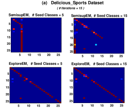
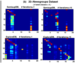
Figure 1: (a) Confusion matrices, varying number of seed classes, for the Delicious_Sports dataset. (b) Confusion matrices, varying the number of EM iterations for the 20-Newsgroups dataset. Each is using Explore-KMeans with the MinMax criterion.

We first consider the value of exploratory learning. With the JS criterion, the exploratory extension gives comparable or improved performance on 8 out of 9 cases. In 5 out of 8 cases the gains are statistically significant. With the simpler MinMax criterion, the exploratory extension results in performance improvements in 6 out of 8 cases, and significantly reduces performance only in one case. The number of classes finally introduced by the MinMax criterion is generally smaller than those introduced by JS criterion.

For both SSL and exploratory systems, the seeded K-Means method gives good results on all 3 datasets. In our MATLAB implementation, the running time of Exploratory EM is longer, but not unreasonably so: on average for 20-Newsgroups dataset Semisup-KMeans took 95 sec. while Explore-KMeans took 195 sec. and for Reuters dataset, Semisup-KMeans took 7 sec. while Explore-KMeans took 28 sec.

We can also see that Random criterion shows significant improvements over the baseline SemisupEM method in 4 out of 9 cases. While Exploratory EM method with MinMax and JS criterion shows significant improvements in 5 out of 9 cases. In terms of magnitude of improvements, JS is superior to Random criterion.

Next we compare Exploratory EM with baseline named “SemisupEM with $m$ extra classes”. The last column of Table 1 shows the best performance of this baseline by varying $m$ = {0, 1, 2, 5, 10, 20, 40}, and choosing that value of $m$ for which seed class F1 is maximum. Since the “best $m$ extra classes” baseline is making use of the test labels to pick right number of classes, it cannot be used in practice; however Exploratory EM methods produce comparable or better performance with this strong baseline.

To better understand the qualitative behavior of our methods, we conducted some further experiments with Semisup-KMeans with the MinMax criterion (which appears to be a reasonable baseline method.) We constructed confusion matrices for the classification task, to check how different methods perform on each dataset. Figure 1 (a) shows the confusion matrices for SemisupEM (top row) and Exploratory EM (bottom row) with five and fifteen seeded classes. We can see that SemisupEM with only five seed classes clearly confuses the unexpected classes with the seed classes, while Exploratory EM gives better quality results. Having seeds for more classes helps both SemisupEM and Exploratory EM, but SemisupEM still tends to confuse the unexpected classes with the seed classes. Figure 1 (b) shows similar results on the 20-Newsgroups dataset, but shows the confusion matrix after 1 iteration and after 15 iterations of EM. It shows that SemisupEM after 15 iterations has made limited progress in improving its classifier when compared to Exploratory EM.

Finally, we compare the two class creation criteria, and show a somewhat larger range of seeded classes, ranging from 5 to 15 (out of 20 actual classes). In Figure 2 each of the confusion-matrices is annotated with the strategy, the number of seed classes and the number of classes produced. (E.g., plot “MinMax-C5(23)” describes Explore-KMeans with MinMax criterion and 5 seed classes which produces 23 clusters.) We can see that MinMax criterion usually produces a more reasonable number of clusters, closer to the ideal value of 20; however, performance of the JS method in terms of seed class accuracy is comparable to the MinMax method.

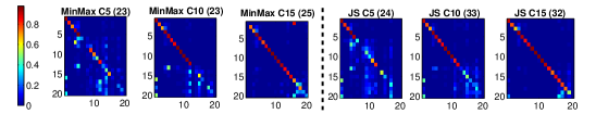
Figure 2: 20-Newsgroups dataset : Comparison of MinMax vs. JS criterion for ExploreEM

These trends are also shown quantitatively in Figure 4, which shows the result of varying the number of seeded classes (with five seeds per class) for Explore-KMeans and Semisup-KMeans; the top shows the effect on F1, and the bottom shows the effect on the number of classes produced (for Explore-KMeans only). Figure 4 shows a similar effect on the Delicious_Sports dataset: here we systematically vary the number of seeded classes (using 5 seeds per seeded class, on the top), and also vary the number of seeds per class (using 10 seeded classes, on the bottom.) The left-hand side compares the F1 for Semisup-KMeans and Explore-KMeans, and the right-hand side shows the number of classes produced by Explore-KMeans. For all parameter settings, Explore-KMeans is better than or comparable to Semisup-KMeans in terms of F1 on seed classes.

3.2 Comparison with the Chinese Restaurant Process

As discussed in Section 2.6.3, a seeded version of the Chinese Restaurant Process with Gibbs sampling (CRP−Gibbs) is an alternative exploratory learning algorithm. In this section we compare the performance of CRP−Gibbs with Explore-KMeans and Semisup-KMeans. We consider two versions of CRP-Gibbs, one using the standard CRP and one using our proposed modified CRP criterion for new class creation that is sensitive to the near-uniformity of instance’s posterior class distribution. CRP-Gibbs uses the same instance representation as our K-Means variants i.e. $L_{1}$ normalized TFIDF features.

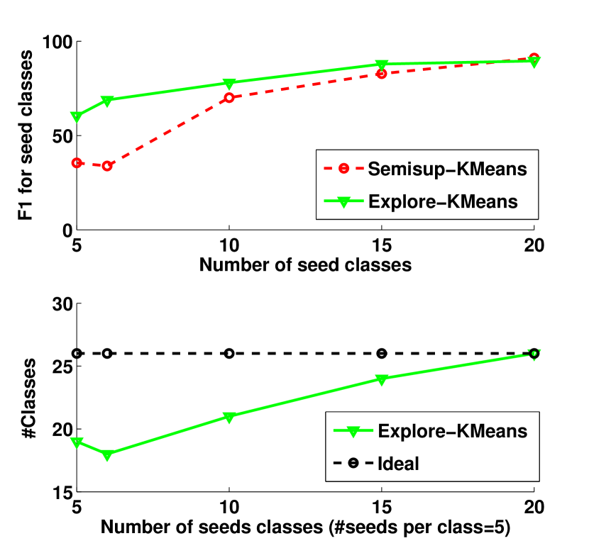
Figure 3: 20-Newsgroups dataset: varying the number of seed classes (using the MinMax criterion).

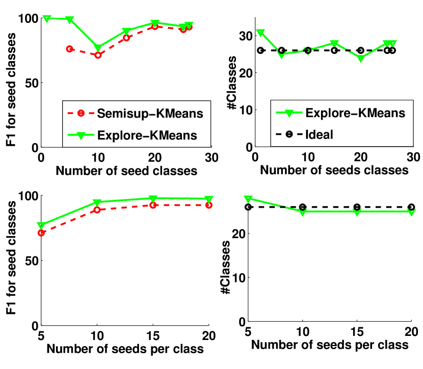
Figure 4: Delicious Sports dataset: Top, varying the number of seed classes (with five seeds per class). Bottom, varying the number of seeds per class (with 10 seed classes).

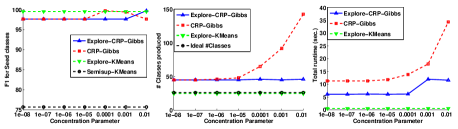
Figure 5: Delicious_Sports dataset: Varying the concentration parameter, with five seed classes.

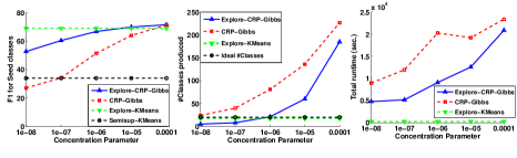
Figure 6: 20-Newsgroups dataset: Varying concentration parameter, with six seed classes.

It is well-known that CRP is sensitive to the concentration parameter $P_{\it new}$. Figures 5 and 6 show the performance of all the exploratory methods, as well as Semisup-KMeans, as the concentration parameter is varied from $10^{-8}$ to $10^{-2}$. (For Explore-KMeans and Semisup-KMeans methods, this parameter is irrelevant). We show F1, the number of classes produced, and run-time (which is closely related to the number of classes produced.) The results show that a well-tuned seeded CRP-Gibbs can obtain good F1-performance, but at the cost of introducing many unnecessary clusters. The modified Explore-CRP-Gibbs performs consistently better, but not better than Explore-KMeans, and Semisup-KMeans performs the worst.

4 Related Work

In this paper we describe and evaluate a novel multiclass SSL method that is more robust when there are unanticipated classes in the data—or equivalently, when the algorithm is given seeds from only some of the classes present in the data. To the best of our knowledge this specific problem has not been explored in detail before, even though in real-world settings, there can be unanticipated (and hence unseeded) classes in any sufficiently large-scale multiclass SSL task.

More generally, however, it has been noted before that SSL may suffer due to the presence of unexpected structure in the data. For instance, Nigam et al’s early work on SSL based EM with multinomial Naive Bayes [21] noted that adding too much unlabeled data sometimes hurt performance on SSL tasks, and discusses several reasons this might occur, including the possibility that there might not be a one-to-one correspondence between the natural mixture components (clusters) and the classes. To address this problem, they considered modeling the positive class with one component, and the negative class with a mixture of components. They propose to choose the number of such components by cross-validation; however, this approach is relatively expensive, and inappropriate when there are only a small number of labeled examples (which is a typical case in SSL). More recently, McIntosh [18] described heuristics for introducing new “negative categories” in lexicon bootstrapping, based on a domain-specific heuristic for detecting semantic drift with distributional similarity metrics. Our setting is broadly similar to these works, except that we consider this task in a general multiclass-learning setting, and do not assume seeds from an explicitly-labeled “negative” class, which is a mixture; instead, we assume seeds from known classes only. Thus we assume that data fits a mixture model with a one-to-one correspondence with the classes, but only after the learner introduces new classes hidden in the data. We also explore this issue in much more depth experimentally, by systematically considering the impact of having too few seed classes, and propose and evaluate a solution to the problem. There has also been substantial work in the past to automatically decide the right “number of clusters” in unsupervised learning [11, 22, 15, 7, 19, 27]. Many of these techniques are built around K-Means and involve running it multiple times for different values of K. Exploratory learning differs in that we focus on a SSL setting, and evaluate specifically the performance difference on the seeded classes, rather than overall performance differences.

There is also a substantial body of work on constrained clustering; for instance, Wagstaff et al [26] describe a constrained clustering variant of K-Means “must-link” and “cannot-link” constraints between pairs. This technique changes the cluster assignment phase of K-Means algorithm by assigning each example to the closest cluster such that none of the constraints are violated. SSL in general can be viewed as a special case of constrained clustering, as seed labels can be viewed as constraints on the clusters; hence exploratory learning can be viewed as a subtype of constrained clustering, as well as a generalization of SSL. However, our approach is different in the sense that there are more efficient methods for dealing with seeds than arbitrary constraints.

In this paper we focused on EM-like SSL methods. Another widely-used approach to SSL is label propagation. In the modified adsorption algorithm [25], one such graph-based label propagation method, each datapoint can be marked with one or more known labels, or a special dummy label meaning “none of the above”. Exploratory learning is an extension that applies to a different class of SSL methods, and has some advantages over label propagation: for instance, it can be used for inductive tasks, not only transductive tasks. Exploratory EM also provides more information by introducing multiple “dummy labels” which describe multiple new classes in the data.

A third approach to SSL involves unsupervised dimensionality reduction followed by supervised learning (e.g., [8]). Although we have not explored their combination, these techniques are potentially complementary with exploratory learning, as one could also apply EM-like methods, in a lower-dimensional space (as is typically done in spectral clustering). If this approach were followed then an exploratory learning method like Exploratory EM could be used to introduce new classes, and potentially gain better performance, in a semi-supervised setting.

One of our benchmark tasks, entity classification, is inspired by the NELL (Never Ending Language Learning) system [5]. NELL performs broad-scale multiclass SSL. One subproject within NELL [20] uses a clustering technique for discovering new relations between existing noun categories—relations not defined by the existing hand-defined ontology. Exploratory learning addresses the same problem, but integrates the introduction of new classes into the SSL process. Another line of research considers the problem of “open information extraction”, in which no classes or seeds are used at all [28, 12, 9]. Exploratory learning, in contrast, can exploit existing information about classes of interest and seed labels to improve performance.

Another related area of research is novelty detection. Topic detection and tracking task aims to detect novel documents at time $t$ by comparing them to all documents till time $t-1$ and detects novel topics. Kasiviswanathan et al. [16] assumes the number of novel topics is given as input to the algorithm. Masud et al. [17] develop techniques on streaming data to predict whether next data chunk is novel or not. Our focus is on improving performance of semi-supervised learning when the number of new classes is unknown. Bouveyron [3] worked on the EM approach to model unknown classes, but the entire EM algorithm is run for multiple numbers of classes. Our algorithm jointly learns labels as well as new classes. Schölkopf et al. [24] defines a problem of learning a function over the data space that isolates outliers from class instances. Our approach is different in the sense we do not focus on detecting outliers for each class.

5 Conclusion

In this paper, we investigate and improve the robustness of SSL methods in a setting in which seeds are available for only a subset of the classes—the subset of most interest to the end user. We performed systematic experiments on fully-labeled multiclass problems, in which the number of classes is known. We showed that if a user provides seeds for only some, but not all, classes, then SSL performance is degraded for several popular EM-like SSL methods (semi-supervised multinomial Naive Bayes, seeded K-Means, and a seeded version of mixtures of von Mises-Fisher distributions). We then described a novel extension of the EM framework called Exploratory EM, which makes these methods much more robust to unseeded classes. Exploratory EM introduces new classes on-the-fly during learning based on the intuition that hard-to-classify examples—specifically, examples with a nearly-uniform posterior class distribution—should be assigned to new classes. The exploratory versions of these SSL methods often obtained dramatically better performance—e.g., on Delicious_Sports dataset up to 90% improvements in F1, on 20-Newsgroups dataset up to 27% improvements in F1, and on Reuters dataset up to 200% improvements in F1. In comparative experiments, one exploratory SSL method, Explore-KMeans, emerged as a strong baseline approach.

Because Exploratory EM is broadly similar to non-parametric Bayesian approaches, we also compared Explore-KMeans to a seeded version of an unsupervised mixture learner that explores differing numbers of mixture components with the Chinese Restaurant process (CRP). Explore-KMeans is faster than this approach, and more accurate as well, unless the parameters of the CRP are very carefully tuned. Explore-KMeans also generates a model that is more compact, having close to the true number of clusters. The seeded CRP process can be improved, moreover, by adapting some of the intuitions of Explore-KMeans, in particular by introducing new clusters most frequently for hard-to-classify examples (those with nearly-uniform posteriors).

The exploratory learning techniques we described here are limited to problems where each data point belongs to only one class. An interesting direction for future research can be to develop such techniques for multi-label classification, and hierarchical classification. Another direction can be create more scalable parallel versions of Explore-KMeans for much larger datasets, e.g., large-scale entity-clustering task.

Acknowledgments:

This work is supported in part by the Intelligence Advanced Research Projects Activity (IARPA) via Air Force Research Laboratory (AFRL) contract number FA8650-10-C-7058. The U.S. Government is authorized to reproduce and distribute reprints for Governmental purposes notwithstanding any copyright annotation thereon. This work is also partially supported by the Google Research Grant. The views and conclusions contained herein are those of the authors and should not be interpreted as necessarily representing the official policies or endorsements, either expressed or implied, of Google, IARPA, AFRL, or the U.S. Government.

References

- [1] A. Banerjee, I. S. Dhillon, J. Ghosh, and S. Sra. Clustering on the unit hypersphere using von mises-fisher distributions. In JMLR, 2005.
- [2] S. Basu, A. Banerjee, and R. Mooney. Semi-supervised clustering by seeding. ICML, 2002.
- [3] C. Bouveyron. Adaptive mixture discriminant analysis for supervised learning with unobserved classes. 2010.
- [4] K. P. Burnham and D. R. Anderson. Multimodel inference understanding aic and bic in model selection. Sociological methods & research, 2004.
- [5] A. Carlson, J. Betteridge, R. C. Wang, E. R. Hruschka, Jr., and T. M. Mitchell. Coupled semi-supervised learning for information extraction. In WSDM, 2010.
- [6] G. Celeux and G. Govaert. A classification em algorithm for clustering and two stochastic versions. Computational statistics & Data analysis, 1992.
- [7] M. M.-T. Chiang and B. Mirkin. Intelligent choice of the number of clusters in k-means clustering: An experimental study with different cluster spreads. J. Classification, 2010.
- [8] B. Dalvi and W. Cohen. Very fast similarity queries on semi-structured data from the web. In SDM. 2013.
- [9] B. Dalvi, W. Cohen, and J. Callan. Websets: Extracting sets of entities from the web using unsupervised information extraction. In WSDM, 2012.
- [10] X. W. Deng Cai and X. He. Probabilistic dyadic data analysis with local and global consistency. ICML, 2009.
- [11] H. Dutta, R. Passonneau, A. Lee, A. Radeva, B. Xie, D. Waltz, and B. Taranto. Learning parameters of the k-means algorithm from subjective human annotation. FLAIRS, 2011.
- [12] O. Etzioni, M. Cafarella, D. Downey, S. Kok, A.-M. Popescu, T. Shaked, S. Soderland, D. S. Weld, and A. Yates. Web-scale information extraction in knowitall. In WWW, 2004.
- [13] N. Friedman, M. Ninio, I. Pe’er, and T. Pupko. A structural em algorithm for phylogenetic inference. Journal of Computational Biology, 2002.
- [14] D. Griffiths and M. Tenenbaum. Hierarchical topic models and the nested chinese restaurant process. In NIPS, 2004.
- [15] G. Hamerly and C. Elkan. Learning the k in k-means. In NIPS, 2003.
- [16] S. P. Kasiviswanathan, P. Melville, A. Banerjee, and V. Sindhwani. Emerging topic detection using dictionary learning. In CIKM, 2011.
- [17] M. M. Masud, J. Gao, L. Khan, J. Han, and B. Thuraisingham. Integrating novel class detection with classification for concept-drifting data streams. In ECML/PKDD. 2009.
- [18] T. McIntosh. Unsupervised discovery of negative categories in lexicon bootstrapping. EMNLP, 2010.
- [19] D. A. Menasce, V. A. F. Almeida, R. Fonseca, and M. A. Mendes. A methodology for workload characterization of e-commerce sites. EC, 1999.
- [20] T. Mohamed, E. Hruschka Jr, and T. Mitchell. Discovering relations between noun categories. In EMNLP, 2011.
- [21] K. Nigam, A. McCallum, S. Thrun, and T. Mitchell. Text classification from labeled and unlabeled documents using em. Machine learning, 2000.
- [22] D. Pelleg, A. Moore, et al. X-means: Extending k-means with efficient estimation of the number of clusters. In ICML, 2000.
- [23] J. Rennie. 20-newsgroup dataset, 2008.
- [24] B. Schölkopf, R. C. Williamson, A. J. Smola, J. Shawe-Taylor, and J. Platt. Support vector method for novelty detection. NIPS, 2000.
- [25] P. Talukdar and K. Crammer. New regularized algorithms for transductive learning. In ECML-PKDD. 2009.
- [26] K. Wagstaff, C. Cardie, S. Rogers, and S. Schrodl. Constrained k-means clustering with background knowledge. ICML, 2001.
- [27] M. Welling and K. Kurihara. Bayesian k-means as a maximization-expectation algorithm. In ICDM, 2006.
- [28] A. Yates, M. Cafarella, M. Banko, O. Etzioni, M. Broadhead, and S. Soderland. Textrunner: Open information extraction on the web. In NAACL, 2007.