Fractional vortex molecules and vortex polygons
in a baby Skyrme model

Abstract

We construct a molecule of fractional vortices with fractional topological lump charges as a baby Skyrmion with the unit topological lump charge in the anti-ferromagnetic (or XY) baby Skyrme model, that is, an $O(3)$ sigma model with a four derivative term and an anti-ferromagnetic or XY-type potential term quadratic in fields. We further construct configurations with topological lump charges $Q\leq 7$ and find that bound states of vortex molecules constitute regular polygons with $2Q$ vertices as vortices, where the rotational symmetry $SO(2)$ in real space is spontaneously broken into a discrete subgroup ${\bf Z}_{Q}$. We also find metastable and arrayed bound states of fractional vortices for $Q=5,6$. On the other hand, we find for $Q=7$ that the regular polygon is metastable and the arrayed bound state is stable. We calculate binding energies of all configurations.

I Introduction

Vortices are topological solitons present in various physical systems from field theory Manton:2004tk and cosmological models Vilenkin:2000 to condensed matter systems Volovik:2003 . In particular, they play essential roles in condensed matter systems such as superconductors, superfluids, magnetism, quantum Hall states, nematic liquids, optics, and so on. One of the exotic aspects common in condensed matter systems but not familiar in high energy physics and cosmology are vortex molecules, which have been studied in multi-component Bose-Einstein condensates (BECs) Son:2001td ; Kasamatsu:2004 ; Kasamatsu:2005 ; Eto:2012rc ; Cipriani:2013nya ; Cipriani:2013wia ; Eto:2013 , multi-gap superconductors Babaev:2002 ; Goryo:2007 ; Nitta:2010yf , superfluid ³He (as a double core vortex) Volovik:2003 , and nonlinear optics optics . In the cases of BECs Son:2001td and superconductors Tanaka:2001 , fractional vortices in two different components with fractional topological charges constitute a meson-like bound state with the unit topological charge in total. However, a crucial difference between these two systems is that a repulsion between vortices is exponentially suppressed in superconductors due to the Higgs mechanism in the presence of a gauge field while a repulsion between vortices is polynomially reduced in BECs Eto:2011wp in the absence of a gauge field. Consequently, vortex molecules are stable and visible in BECs because of a balance between the vortex repulsion and the domain wall tension, while in superconductors they can be seen, in principle, only at temperatures above a certain critical temperature by a mechanism similar to the Berezinskii-Kosterlitz-Thouless transition Goryo:2007 ; Nitta:2010yf . However, stable vortex molecules in BECs are global vortices winding around a global $U(1)$ symmetry, and consequently their energies are logarithmically divergent with respect to the system size; they are infinitely heavy in infinite space, and thereby they are not very realistic in high energy physics or cosmology.

In this paper, we propose a field theoretical model admitting a vortex molecule with finite energy, motivated by these condensed matter systems. We consider an $O(3)$ nonlinear sigma model on the target space $S^{2}$ in $d=2+1$ dimensions, described by a unit three-vector of scalar fields ${\bf n}(x)=(n_{1}(x),n_{2}(x),n_{3}(x))$ with the constraint ${\bf n}^{2}=1$, which is equivalent to a ${\bf C}P^{1}$ model. The $O(3)$ model admits lumps or sigma model instantons characterized by $\pi_{2}(S^{2})\simeq{\bf Z}$ Polyakov:1975yp as a relative of vortices. We consider a potential term motivated by condensed matter systems admitting vortex molecules. The potential terms make lumps unstable against shrinkage, in general, as can be inferred from the scaling argument Derrick:1964ww , so we also consider a four derivative (Skyrme) term, by which the lumps are stabilized to become baby Skyrmions Piette:1994ug . In the context of baby Skyrmions, the potential terms of the type $V=m^{2}(1-n_{3})$ Piette:1994ug or of the type $V=m^{2}(1-n_{3}^{2})$ Kudryavtsev:1997nw ; Weidig:1998ii ; Harland:2007pb ; Nitta:2012kk have already been studied. The latter admits two discrete vacua $n_{3}=\pm 1$ and a domain wall interpolating between them Abraham:1992vb ; Kudryavtsev:1997nw ; Harland:2007pb ; Nitta:2012kj , and a baby Skyrmion is in the shape of a twisted closed domain wall Weidig:1998ii ; Kobayashi:2013ju . In our previous papers Nitta:2012xq ; Nitta:2012wi ; Kobayashi:2013ju , we considered both types of potential terms $V=m^{2}(1-n_{3}^{2})+\beta^{2}n_{1}$ in the regime $\beta\ll m$. In this case, a straight domain wall can absorb lumps as sine-Gordon kinks Nitta:2012xq ; Nitta:2012wi ; Kobayashi:2013ju , and a baby Skyrmion is in the form of a domain wall ring with a sine-Gordon kink Kobayashi:2013ju . In condensed matter physics, the quadratic potential admitting two vacua is known as the Ising-type in ferromagnets, so we may refer to this model as the Ising (or ferromagnetic) baby Skyrme model.

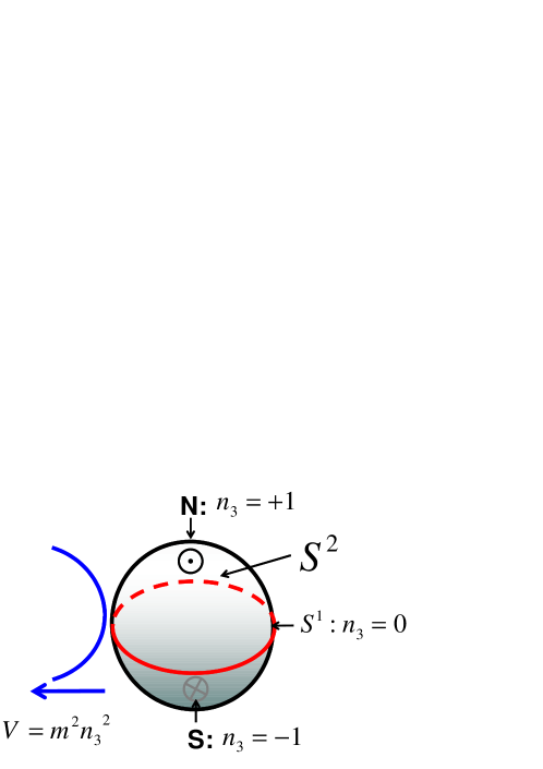
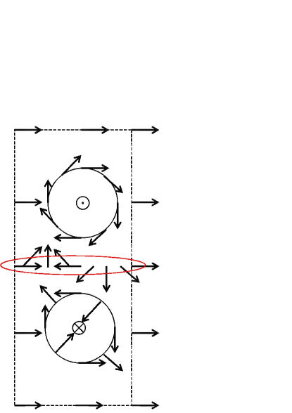
Figure 1: (a) The target space and the potential. (b) A vortex molecule as one lump. Here, $\leftarrow$, $\downarrow$, $\rightarrow$ and $\uparrow$ represent ${\bf n}=(-1,0,0),(0,-1,0),(1,0,0)$ and $(0,1,0)$, respectively. The north and south poles ${\bf n}=(0,0,1)$ and $(0,0,-1)$ are denoted by $\odot$ and $\otimes$, respectively.

Here, we consider a potential of the XY-type or of anti-ferromagnets, $V=m^{2}n_{3}^{2}$ Jaykka:2010bq . The model can be referred as the XY (or anti-ferromagnetic) baby Skyrme model. The vacua characterized by $n_{3}=0$ are $S^{1}$ at the equator of the target space $S^{2}$, as in Fig. 1 (a). One lump solution is schematically drawn in Fig. 1 (b), where we chose ${\bf n}=(1,0,0)$ as the vacuum at the boundary. One can find two separated half lumps (merons) whose centers are mapped to the north and south poles ${\bf n}=(0,0,\pm 1)$ of the target space $S^{2}$. These half lumps are separated because the vacua $S^{1}$ appear between them as indicated by an ellipse in Fig. 1 (b). Therefore, a lump is non-axisymmetric, unlike those for the massless case and the Ising-type case with $\beta=0$ in which lumps are axisymmetric. There, the vacuum $U(1)$ winds (counter)clockwise between the two half lumps so that these half lumps are (anti-)global vortices. While isolated (anti-)global vortices have logarithmically divergent energy in the infinite system size, a pair of global and anti-global vortices have finite energy. They attract each other and collapse in the absence of the Skyrme term, while the Skyrme term forms a vortex molecule. We numerically construct fractional vortex molecules with $1\leq Q\leq 7$ by a relaxation method. The configuration of $Q=1$, in fact, looks what we expected. For $Q=2$, we find that two molecules face to each other with opposite orientations to constitute a regular square. Since two kinds of constituent vortices are placed at the vertices, the configuration is ${\bf Z}_{2}$ symmetric. For $Q=3$, we find a regular hexagonal structure of vortex molecules like a benzene. This is ${\bf Z}_{3}$ symmetric. The configurations with $Q=2,3$ resemble those recently found in a two-component BEC under rotation Cipriani:2013nya . Furthermore, for $Q=4,5,6$, we find regular octagonal, decagonal, and dodecagonal structures of fractional vortices with ${\bf Z}_{4}$, ${\bf Z}_{5}$, ${\bf Z}_{6}$ symmetries. Therefore, in general, we expect, for the topological charge $Q$, a polygon with $2Q$ fractional vortices at vertices with ${\bf Z}_{Q}$ symmetry Jaykka:2010bq . We also find metastable and arrayed bound states of fractional vortices for $Q=5,6$. These configurations are obtained by squeezing the corresponding stable polygons, and they have slightly higher energies. We also find that the regular polygon is metastable and the arrayed bound state is stable for $Q=7$. Finally, we calculate binding energies of all the configurations.

Conventional lumps in the massless $O(3)$ sigma model are invariant under a combination of the $U(1)$ rotation of the target space and the space rotation. The lumps spontaneously break the other linear combination of the two $U(1)$ symmetries. On the other hand, our solutions spontaneously break the purely space rotation. Note that non-axisymmetric configurations were known before for higher topological charges in the baby Skyrme model Delsate:2012hz , while even one baby Skyrmion is non-axisymmetric in our model. In this regard, our solutions are similar to those in Ref. Jaykka:2011ic , in which non-axisymmetric molecular configurations were found in the model with a more complicated potential. We would like to emphasize that our potential is quite common in anti-ferromagnets and two-component BECs and that it is natural.

A closely related model is a $U(1)$ gauged supersymmetric ${\bf C}P^{1}$ model where a rotation along the $n_{3}$ axis is gauged Bagger:1982fn . The gauge symmetry induces the potential $V=m^{2}n_{3}^{2}$ known as the D-term potential where supersymmetry requires $m$ to coincide with the gauge coupling $e$. In this model, a lump is decomposed into two fractional gauged Bogomol’nyi-Prasad-Sommerfield (BPS) vortices, and these two vortices can be placed with arbitrary separation because no force is present between BPS vortices Schroers:1995he ; Nitta:2011um . Each constituent vortex carries half of the lump charge characterized by $\pi_{2}(S^{2})$, as in our model. A set of fractional vortices carrying the total unit charge was also found in supersymmetric gauge theories and sigma models Eto:2009bz .

This paper is organized as follows. After our model is explained in Sec. II, we give numerical solutions of vortex molecules in Sec. III. Section IV is devoted to a summary and discussion.

II The model

We consider an $O(3)$ sigma model in $d=2+1$ dimensions described by a three vector of scalar fields ${\bf n}(x)=(n_{1}(x),n_{2}(x),n_{3}(x))$ with a constraint ${\bf n}\cdot{\bf n}=1$. The Lagrangian of our model is given by

$${\cal L}=\frac{1}{2}\partial_{\mu}{\bf n}\cdot\partial^{\mu}{\bf n}-{\cal L}_{4}({\bf n})-V({\bf n}),\quad$$ (1)

with $\mu=0,1,2$. Here, the four derivative (baby Skyrme) term is expressed as

$${\cal L}_{4}({\bf n})=\kappa F_{\mu\nu}^{2}=\kappa\left[{\bf n}\cdot(\partial_{\mu}{\bf n}\times\partial_{\nu}{\bf n})\right]^{2}=\kappa(\partial_{\mu}{\bf n}\times\partial_{\nu}{\bf n})^{2},\quad F_{\mu\nu}\equiv{\bf n}\cdot(\partial_{\mu}{\bf n}\times\partial_{\nu}{\bf n}).$$ (2)

In this paper, we take the potential term to be Jaykka:2010bq

$$V({\bf n})=m^{2}n_{3}^{2}.$$ (3)

This potential is known in anti-ferromagnets and the XY model, while the potential in the form of ferromagnets $m^{2}(1-n_{3}^{2})$ was studied before in Refs. Weidig:1998ii ; Kudryavtsev:1997nw ; Harland:2007pb ; Nitta:2012kk . The energy density of static configurations is

$$\mathcal{E}\equiv\frac{1}{2}(\partial_{a}{\bf n}\cdot\partial^{a}{\bf n})+{\cal L}_{4}({\bf n})+V({\bf n}),\quad(a=1,2).$$ (4)

Itroducing the projective coordinate $u(\in{\bf C})$ of ${\bf C}P^{1}$ by

$$n_{i}=\phi^{\dagger}\sigma_{i}\phi,\quad\phi^{T}=(1,u)/\sqrt{1+|u|^{2}},$$ (5)

the Lagrangian (1) can be rewritten in the form of the ${\bf C}P^{1}$ model with potential terms, given by

$${\cal L}=2\frac{\partial_{\mu}u^{*}\partial^{\mu}u}{(1+|u|^{2})^{2}}-8\kappa\frac{(\partial_{\mu}u^{*}\partial^{\mu}u)^{2}-|\partial_{\mu}u\partial^{\mu}u|^{2}}{(1+|u|^{2})^{4}}-V$$ (6)

$$V=m^{2}D_{3}^{2},\quad D_{3}\equiv\frac{1-|u|^{2}}{1+|u|^{2}}=n_{3},$$ (7)

Here, $g_{uu^{*}}=1/(1+|u|^{2})^{2}$ is the Kähler (Fubini-Study) metric of ${\bf C}P^{1}$, $g^{uu^{*}}=(1+|u|^{2})^{2}$ is its inverse, and $D_{i}=n_{i}$ are the moment maps (or the Killing potentials) of the $SU(2)$ isometry generated by $\sigma_{i}$. If we gauge the isometry generated by the generator $\sigma_{3}$ with gauge coupling $e$, the potential $V=e^{2}D_{3}^{2}$ (with $m=e$) is known as the D-term potential in the supersymmetric $U(1)$ gauged ${\bf C}P^{1}$ model Bagger:1982fn .

III Vortex molecules

The topological charge of the lump $\pi_{2}(S^{2})\simeq{\bf Z}$ is given by

$$Q = \frac{1}{4\pi}\int d^{2}x\>F_{12}=\frac{1}{4\pi}\int d^{2}x\>{\bf n}\cdot(\partial_{1}{\bf n}\times\partial_{2}{\bf n})=\frac{1}{4\pi}\int d^{2}x\>\epsilon_{ijk}n_{i}\partial_{1}n_{j}\partial_{2}n_{k}$$ (8)

$$= \frac{1}{2\pi}\int d^{2}x{i(\partial_{1}u^{*}\partial_{2}u-\partial_{2}u^{*}\partial_{1}u)\over(1+|u|^{2})^{2}}.$$

In the presence of the potential, a lump is unstable to shrinking from the Derick’s scaling argument Derrick:1964ww . It can be stabilized in the presence of the baby Skyrme term, resulting in a baby Skyrmion.

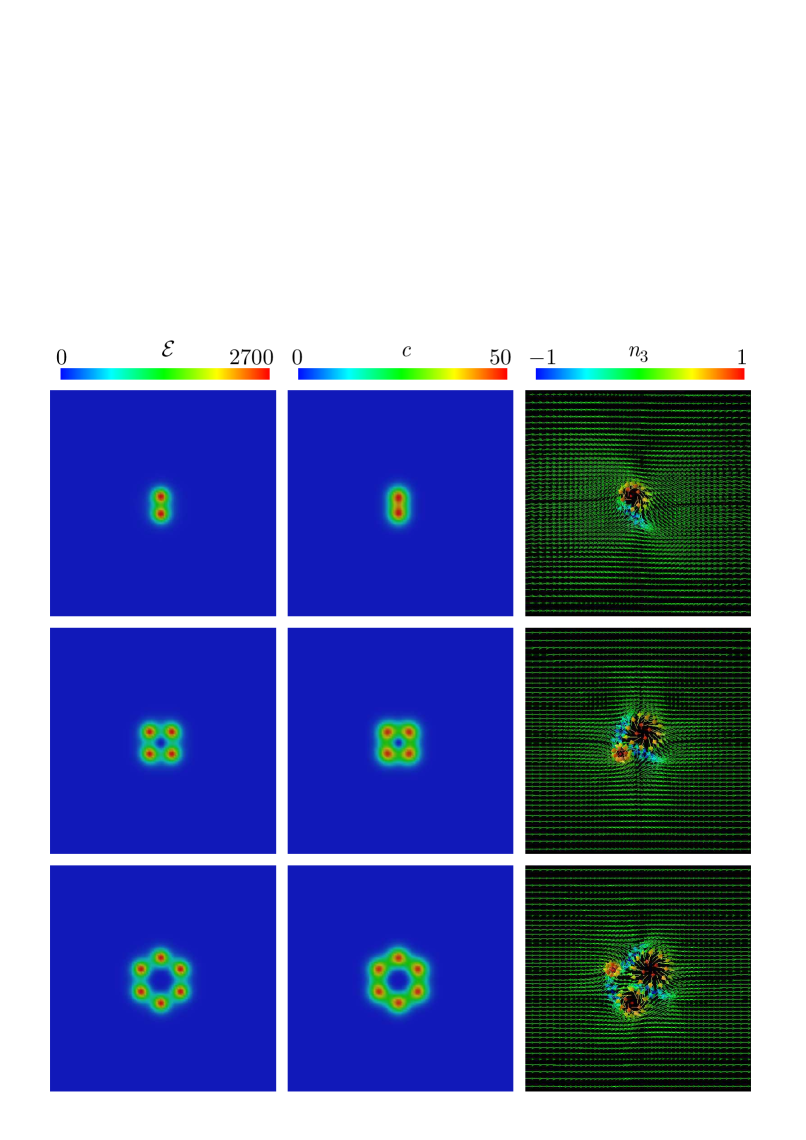
Figure 2: Bound states of fractional vortex molecules in the region $-1.16<x_{a}<1.16$. The topological charges are $Q=1,2,3$ from top to bottom. The left and middle panels represent the total energy densities $\mathcal{E}(x)$ and the topological charge densities $c(x)\equiv F_{12}/4\pi$, respectively. In the right panels, the arrows denote the scalar fields of the three-vector ${\bf n}(x)$, where color represents the value of $n_{3}$ from which one can find whether the constituent fractional vortices are of N or S.

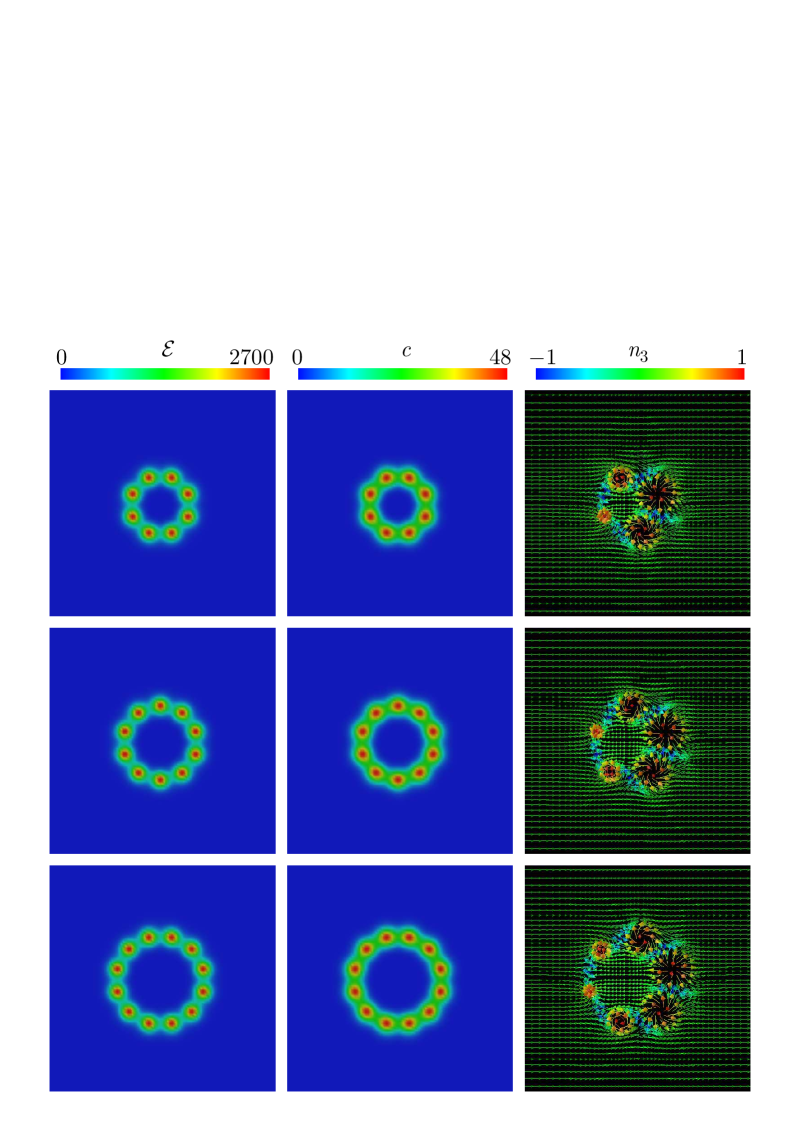
Figure 3: Bound states of fractional vortex molecules in the region $-1.16<x_{a}<1.16$. The topological charges are $Q=4,5,6$ from top to bottom. Details of the plots are the same as those shown in Fig. 2.

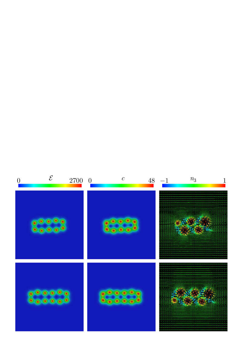
Figure 4: Metastable and arrayed bound states of fractional vortex molecules in the region $-1.16<x_{a}<1.16$. The topological charges are $Q=5,6$ for the top and bottom. Details of the plots are the same as those shown in Fig. 2.

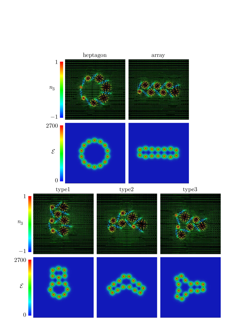
Figure 5: Stable (arrayed) and metastable (heptagon and the other 3 types of) bound states of fractional vortex molecules for the topological charge $Q=7$. The top and bottom panels of each configuration represent the three-vector ${\bf n}(x)$ and the total energy density $\mathcal{E}(x)$, respectively, in the region $-1.16<x_{a}<1.16$.

We construct numerical solutions of fractional vortex molecules with the topological lump charge $1\leq Q\leq 7$. As the numerical parameters, we fix $\kappa=0.002$ and $m^{2}=800$. We obtain the stationary state using the relaxation method: introducing the parameter $\tau$ and the $\tau$-dependence of $n_{i}(\tau)$, and finding the asymptotic solution $n_{i}(\tau\to\infty)$ of the equation

$$\frac{\partial n_{i}}{\partial\tau}=-\frac{\delta\mathcal{E}}{\delta n_{i}},$$ (9)

under the constraint $n_{1}^{2}+n_{2}^{2}+n_{3}^{2}=1$. The detailed numerical procedure is shown in the Appendix A. As the initial state $n_{i}(\tau=0)$, we give the ansatz for $\kappa=m=0$:

$$n_{1}=\cos f(r),\quad n_{2}=-\cos(Q\theta)\sin f(r),\quad n_{3}=\sin(Q\theta)\sin f(r),$$ (10)

with the monotonically decreasing function satisfying

$$f(r\to\infty)\to 0,\quad f(r\to 0)\to\pi.$$ (11)

The topological charge $Q$ given by Eq. (8) is invariant for arbitrary $\tau$.

Our stable solutions are given in Fig. 2 for $Q=1,2,3$ and Fig. 3 for $Q=4,5,6$. For the unit topological charge, $Q=1$, one can find a fractional vortex molecule as we expected; two fractional vortices oppositely wind around the equator $S^{1}$ of the target space $S^{2}$, and their cores are filled by the north $n_{3}=+1$ and south $n_{3}=-1$ poles of $S^{2}$, as can be seen in the plot of $n_{3}$ in Fig. 2. The vacua $S^{1}$ appear between the two half lumps separating them, as can be seen from both the plots of the energy density and topological charge density. Although all of them are (anti-)global vortices having logarithmically divergent energy, a pair them has finite energy. They attract each other, but the Skyrme term prevents the collapse.

For $Q=2$, two vortex molecules face to each other with opposite orientations. Since molecules attract each other with these orientations, they make a bound state to constitute a square. Since the same vortices N or S are placed at each pair of diagonal corners, the configuration is ${\bf Z}_{2}$ axisymmetric.

For $Q=3$, three vortex molecules with six fractional vortices constitute a hexagon with a ${\bf Z}_{3}$ axisymmetry. These structures of $Q=2,3$ resemble those in a vortex lattice recently found in a two-component BEC under rotation Cipriani:2013nya .

For $Q=4,5,6$, the situation is almost the same; i.e., one finds that four, five, and six vortex molecules with eight, ten, and eleven fractional vortices constitute an octagon, decagon, and dodecagon with ${\bf Z}_{4}$, ${\bf Z}_{5}$, ${\bf Z}_{6}$ axisymmetries, respectively.

In general, for the topological charge $Q$, we expect $2Q$ fractional vortices to be placed on a circle in a ${\bf Z}_{Q}$ axisymmetric way. In all the cases, one can see that the topological lump charge density is distributed around the fractional vortices, and each of them carries a half lump charge. The rotational symmetry $SO(2)$ in the $x^{1}$-$x^{2}$ plane is spontaneously broken in all cases to a discrete subgroup ${\bf Z}_{Q}$.

To investigate the stability of vortex polygons, we also choose a randomly placed lump solution

$$u=\sum_{i=1}^{Q}\frac{e^{i\varphi_{i}}}{x_{1}-x_{0i}+ix_{2}-y_{0i}},$$ (12)

as initial states $n_{i}(\tau=0)$ for the relaxation. Here, the projective coordinate $u$ is defined in Eq. (5), and $x_{0i}$, $y_{0i}$, and $\varphi_{i}$ are the real random numbers. The initial state (12) indicates that $Q$ single vortex molecules are placed at $(x_{1},x_{2})=(x_{0i},y_{0i})$ with the angle $\varphi_{i}$, having the topological charge $Q$.

For $Q=1,2,3,4$, any initial state of Eq. (12) relaxes to vortex polygons as shown in Figs. 2 and 3, while, for $Q=5,6$, several initial states relax to metastable states that are different from the vortex decagon and dodecagon, i.e., vortex array states as in Fig. 4, the energy of which is larger than vortex polygon states.

We also find five (meta)stable bound states for $Q=7$ as in Fig. 5. Unlike the cases with $Q<7$, the arrayed bound state is at the absolute minimum. The regular polygon and the other three bound state are metastable at local minima.

$Q$	$E_{\mathrm{grad}}$	$E_{\mathrm{sk}}$	$E_{\mathrm{pot}}$	$E$	$E_{\mathrm{bind}}$
1	29.04	8.840	8.829	46.71
2	53.35	16.96	16.96	87.26	6.153
3	78.45	25.17	25.17	128.8	11.33
4	103.8	33.44	33.44	170.7	16.14
5 (decagon)	129.3	41.73	41.73	212.7	20.79
5 (array)	129.8	41.68	41.68	213.1	20.42
6 (dodecagon)	154.8	50.03	50.03	254.9	25.35
6 (array)	155.2	49.90	49.90	255.0	25.22
7 (heptagon)	180.4	58.34	58.34	297.1	29.86
7 (array)	180.7	58.14	58.13	297.0	29.97
7 (type 1)	181.3	58.29	58.28	297.9	29.09
7 (type 2)	181.2	58.22	58.22	297.6	29.31
7 (type 3)	181.6	58.32	58.32	298.3	28.68

Table 1: Gradient energy $E_{\mathrm{grad}}$, Skyrme energy $E_{\mathrm{sk}}$, potential energy $E_{\mathrm{pot}}$, total energy $E$, and binding energy $E_{\mathrm{bind}}$ for vortex molecules.

Finally, we show in Table 1 the gradient energy $E_{\mathrm{grad}}$, the Skyrme energy $E_{\mathrm{sk}}$, the potential energy $E_{\mathrm{pot}}$, the total energy $E$, and the binding energy $E_{\mathrm{bind}}$ between vortex molecules, defined by

$$\begin{array}[]{c}\displaystyle E_{\mathrm{grad}}=\frac{1}{2}\int d^{2}x\>\partial_{a}{\bf n}\cdot\partial^{a}{\bf n},\quad E_{\mathrm{sk}}=\int d^{2}x\>{\cal L}_{4}({\bf n}),\quad E_{\mathrm{pot}}=\int d^{2}x\>V({\bf n}),\vspace{5pt}\\ \displaystyle E=E_{\mathrm{grad}}+E_{\mathrm{sk}}+E_{\mathrm{pot}},\quad E_{\mathrm{bind}}=QE(Q=1)-E(Q),\end{array}$$ (15)

respectively. In our choice of numerical parameters, the gradient energy is dominant in the total energy. Total energy deviates from the linear relation, i.e., $E(Q)<QE(Q=1)$, and the difference $E_{\mathrm{bind}}$ between $E(Q)$ and $QE(Q=1)$ corresponds to the binding energy between molecules, which dominates in about $10$% of the total energy.

IV Summary and Discussion

We have constructed stable and metastable configurations of the fractional vortex molecules as lumps (baby Skyrmions) in the XY (or anti-ferromagnetic) baby Skyrme model which has the anti-ferromagnetic (XY) potential $V=m^{2}n_{3}^{2}$. We have found that, for the unit charge $Q=1$, two fractional vortices whose centers are filled by the north and south poles of the target space are placed within a certain distance. We have found that, for $Q=2,3,4,5$ and $6$, bound states of two, three, four, five, and six vortex molecules constitute quadrangle, hexagonal, octagonal, decagonal, and dodecagonal vortex configurations, respectively. At least up to this topological number, ${\bf Z}_{Q}$ symmetric vortex molecule configurations appear for the topological charge $Q$. Our configurations are all non-axisymmetric, and they spontaneously break the rotational symmetry in the $x$-$y$ plane. While all vortex polygons are stable and at global minima, we have also found metastable and arrayed bound states of fractional vortices for $Q=5,6$, which are obtained by squeezing the corresponding stable polygons and have slightly higher energies. We also find for $Q=7$ that the arrayed bound state is at the absolute minimum and the regular polygon together with the other three bound state is metastable at a local minimum, unlike the cases with $Q<7$ Finally, we have calculated the binding energies of all the configurations.

As denoted in the Introduction, similar configurations of vortex molecules are present in condensed matter systems, such as two component BECs, described by two condensations (scalar fields) $\phi_{1}(x)$ and $\phi_{2}(x)$ with the internal coherent (Josephson) coupling $\beta^{2}\phi_{1}^{*}\phi_{2}+$ c.c. Son:2001td ; Kasamatsu:2004 ; Kasamatsu:2005 ; Eto:2012rc ; Cipriani:2013nya , where a four derivative term is not present. In these cases, the vortex molecules are global vortices, that is, they wind around a global $U(1)$ symmetry. If we gauge the common phase of the two components, they become semi-local vortices. If we send the scalar coupling and gauge coupling to infinity with keeping the internal coherent coupling, we obtain our model except for the Skyrme term where the Josephson coupling $\beta^{2}\phi_{1}^{*}\phi_{2}+$ c.c reduces to $\beta^{2}n_{1}$, which we did not consider in this paper. We expect that semi-local vortices, keeping the couplings, can make a stable vortex molecule if one properly adds a four derivative term.

In the ${\bf C}P^{1}$ model with a ferromagnetic potential, a Q-lump solution is known Leese:1991hr , in which a $U(1)$ Nambu-Goldstone mode associated with the spontaneously broken $U(1)$ internal symmetry of the rotation in the $n_{1}$-$n_{2}$ plane in the target space is rotating in time. In our case, there is a Nambu-Goldstone mode associated with the spontaneously broken rotational symmetry in real space, instead of an internal $U(1)$ Nambu-Goldstone mode. Consequently, we may have a Q-lump in our case as a spinning molecule.

If we promote our configuration linearly in $d=3+1$ dimensions, it becomes a bound state of two cosmic strings. As usual, the solution breaks translational symmetries in two transverse directions, resulting in two translational zero modes which propagate along the string. One added feature of our solutions is the existence of a Nambu-Goldstone mode associated with the spontaneously broken rotational symmetry along the string, resulting in a twisting wave propagating along the string. This is known as a “twiston” in two-gap superconductors Tanaka:2007 . In cosmology, our solutions can be regarded as some exotic cosmic strings with an internal structure. For instance, it is an interesting question whether or not two such strings reconnect to each other when they collide.

We have found that, for the topological charge $Q$, two kinds of vortices are placed at $2Q$ vertices of a regular polygon, on which a ${\bf Z}_{Q}$ symmetry acts. In this regard, ${\bf Z}_{n}$ symmetric vortex configurations were studied in the Abelian-Higgs model Arthur:1995eh . This is equivalent to vortices on the orbifold ${\bf C}/{\bf Z}_{n}$ studied recently Kimura:2011wh . Vortex polygons have also been studied in hydrodynamics for a long time fluid . Vortex polygons with less than seven vortices as vertices are shown to be stable, while those with more than seven are unstable. One example realized in nature is a vortex hexagon found by Cassini in the north poles of Saturn saturn . In our case too, we have found vortex polygons up to $Q=6$ to be stable, which may be interesting compared with hydrodynamics.

In this paper, we have found a two vortex molecule, that is, a vortex dimer with the unit topological charge in the ${\bf C}P^{1}$ model with the anti-ferromagnetic potential. Stable three or $N$ vortex molecules, that is, vortex trimers or $N$-omers, are present in three or $N$ component BECs Eto:2012rc ; Eto:2013 . Since two components $\phi_{1},\phi_{2}$ with a constraint $|\phi_{1}|^{2}+|\phi_{2}|^{2}=1$ divided by $U(1)$ imply the ${\bf C}P^{1}$ model, the same procedure for $N$ components yields a ${\bf C}P^{N-1}$ model with a certain potential term. While a ${\bf C}P^{N-1}$ generalization of the anti-ferromagnetic type potential was considered before AlvarezGaume:1983ab and was found to admit parallel multiple domain walls Gauntlett:2000ib or domain wall junctions or networks Eto:2005cp ; Eto:2006pg , depending on parameters in the potential, a ${\bf C}P^{N-1}$ generalization of the ferromagnetic (XY-type) of the potential has not been studied thus far in the ${\bf C}P^{N-1}$ model. Skyrme-like terms in the ${\bf C}P^{N-1}$ model were studied before without Ferreira:2008nn ; Liu:2009rz and with Bergshoeff:1984wb ; Eto:2012qda ; Adam:2011hj supersymmetry. A ${\bf C}P^{2}$ or ${\bf C}P^{N-1}$ generalization of the baby Skyrme model with an anti-ferromagnetic potential will admit vortex trimers or $N$-omers, respectively.

Note added

After the paper was published, vortex polygons have been studied in a baby Skyrme model with a different potential Winyard:2013ada .

Appendix A Detailed numerical procedure

Equation (9) can be solved as the steepest descent method:

$$n_{i}(\tau+\Delta\tau)=n_{i}(\tau)-\Delta\tau\frac{\delta\mathcal{E}_{\lambda}(\tau)}{\delta n_{i}(\tau)},$$ (16)

where we omit the spatial dependence of $n_{i}$. $\mathcal{E}_{\lambda}(\tau)$ is defined as

$$\mathcal{E}_{\lambda}(\tau)=\mathcal{E}(\tau)-\lambda(\tau)\{n_{1}(\tau)^{2}+n_{2}(\tau)^{2}+n_{2}^{2}(\tau)\}.$$ (17)

Here, the Lagrange multiplier $\lambda(\tau)$ is fixed to satisfy $n_{1}(\tau+\Delta\tau)^{2}+n_{2}(\tau+\Delta\tau)^{2}+n_{2}(\tau+\Delta\tau)^{2}=1$.

For the space, to approximately consider the infinite space, we use the following scaling transformation:

$$x_{a}=L\tanh^{-1}X_{a}$$ (18)

for $-1<X_{a}<1$, and consider the dependence of $n_{i}$ on $X_{a}$ instead of $x_{a}$, where $L$ is the scaling parameter. We use the square with the $(N+1)^{2}$ grid points. On the $l$-th grid point in the $x_{a}$-direction, the value of $n_{i}(\{(l)_{a}\})$ is defined as

$$n_{i}(\{(l)_{a}\})\equiv n_{i}(\{(\cos(l\pi/N))_{a}\}),$$ (19)

where $n_{i}(\{X_{a}\})$ is the value of $n_{i}$ at $\{X_{a}\}\equiv(X_{1},X_{2})$. We omit the $\tau$-dependence on $n_{i}$ here. For $l=0$ or $N$, which corresponds to infinity, the value of $n_{i}(\{(l)_{a}\})$ is fixed to the ground state:

$$\begin{split}n_{1}(\{(0)_{a}\})=n_{1}(\{(N)_{a}\})=1,\\ n_{2}(\{(0)_{a}\})=n_{2}(\{(N)_{a}\})=0,\\ n_{3}(\{(0)_{a}\})=n_{3}(\{(N)_{a}\})=0.\end{split}$$ (20)

To calculate the spatial derivative of $n_{i}$, we use the spectral collocation method. We expand $n_{i}$ in the Chebyshev polynomials:

$$\tilde{n}_{i}(\{(j)_{a}\})=\frac{1}{N}n_{i}(\{(0)_{a}\})+\frac{2}{N}\sum_{l=1}^{N-1}n_{i}(\{(l)_{a}\})\cos\bigg{(}\frac{lj\pi}{N}\bigg{)}+\frac{(-1)^{j}}{N}n_{i}(\{(N)_{a}\}),$$ (21)

where $\tilde{n}_{i}(\{(j)_{a}\})$ $(0\leq j\leq N)$ is the $j$-th coefficient of the Chebyshev expansion in the $x_{a}$-direction. The first and second spatial derivatives $\partial_{a}n_{i}$ and $\partial_{a}^{2}n_{i}$ can be calculated as

$$\begin{array}[]{c}\displaystyle\partial_{a}n_{i}=\frac{1-X_{a}^{2}}{L}\frac{\partial n_{i}}{\partial X_{a}},\quad\partial_{a}^{2}n_{i}=\frac{(1-X_{a}^{2})^{2}}{L^{2}}\frac{\partial^{2}n_{i}}{\partial X_{a}^{2}}-\frac{2X_{a}(1-X_{a}^{2})}{L^{2}}\frac{\partial n_{i}}{\partial X_{a}},\vspace{5pt}\\ \displaystyle\frac{\partial n_{i}(\{(l)_{a}\})}{\partial X_{a}}=\frac{1}{N}\tilde{m}_{i}(\{(0)_{a}\})+\frac{2}{N}\sum_{j=1}^{N-1}\tilde{m}_{i}(\{(j)_{a}\})\cos\bigg{(}\frac{lj\pi}{N}\bigg{)}+\frac{(-1)^{l}}{N}\tilde{m}_{i}(\{(N)_{a}\}),\vspace{5pt}\\ \displaystyle\frac{\partial^{2}n_{i}(\{(l)_{a}\})}{\partial X_{a}^{2}}=\frac{1}{N}\tilde{s}_{i}(\{(0)_{a}\})+\frac{2}{N}\sum_{j=1}^{N-1}\tilde{s}_{i}(\{(j)_{a}\})\cos\bigg{(}\frac{lj\pi}{N}\bigg{)}+\frac{(-1)^{l}}{N}\tilde{s}_{i}(\{(N)_{a}\}).\end{array}$$ (25)

Coefficients $\tilde{m}_{i}(\{(j)_{a}\})$, and $\tilde{s}_{i}(\{(j)_{a}\})$ satisfy the following recurrence relations:

$$\begin{array}[]{c}\displaystyle\tilde{m}_{i}(\{(j)_{a}\})=\tilde{m}_{i}(\{(j+2)_{a}\})+2(j+1)\tilde{n}_{i}(\{(j+1)_{a}\}),\quad\tilde{m}_{i}(\{(N)_{a}\})=0,\vspace{5pt}\\ \tilde{s}_{i}(\{(j)_{a}\})=\tilde{s}_{i}(\{(j+2)_{a}\})+2(j+1)\tilde{m}_{i}(\{(j+1)_{a}\}),\quad\tilde{s}_{i}(\{(N)_{a}\})=0.\end{array}$$ (28)

Equations (21) and (25) can be calculated by the fast Fourier transform algorithm.

In this paper, we fix $L=0.5$, $N=256$, $\Delta\tau=10^{-6}$.

References

- (1) N. S. Manton and P. Sutcliffe, “Topological solitons,” Cambridge, UK: Univ. Pr. (2004) 493 p.
- (2) A. Vilenkin and E. P. S. Shellard, “Cosmic Strings and Other Topological Defects,” (Cambridge Monographs on Mathematical Physics), Cambridge University Press (July 31, 2000).
- (3) G. E. Volovik, The Universe in a Helium Droplet, Clarendon Press, Oxford (2003).
- (4) D. T. Son, M. A. Stephanov, “Domain walls in two-component Bose-Einstein condensates,” Phys. Rev. A65, 063621 (2002) [cond-mat/0103451].
- (5) K. Kasamatsu, M. Tsubota and M. Ueda, “Vortex Molecules in Coherently Coupled Two-Component Bose-Einstein Condensates,” Phys. Rev. Lett 93, 250406 (2004) [arXiv:cond-mat/0406150].
- (6) K. Kasamatsu, M. Tsubota and M. Ueda, “Vortices in multicomponent Bose-Einstein condensates,” Int. J. Mod. Phys. B 19, 1835 (2005) [arXiv:cond-mat/0505546].
- (7) M. Cipriani and M. Nitta, “Crossover between integer and fractional vortex lattices in coherently coupled two-component Bose-Einstein condensates,” arXiv:1303.2592 [cond-mat.quant-gas].
- (8) M. Cipriani and M. Nitta, “Vortex lattices in three-component Bose-Einstein condensates under rotation: simulating colorful vortex lattices in a color superconductor,” arXiv:1304.4375 [cond-mat.quant-gas].
- (9) M. Eto and M. Nitta, “Vortex trimer in three-component Bose-Einstein condensates,” Phys. Rev. A 85, 053645 (2012) [arXiv:1201.0343 [cond-mat.quant-gas]].
- (10) M. Eto and M. Nitta, “Vortex graphs as -omers and Skyrmions in -component Bose-Einstein condensates,” arXiv:1303.6048 [cond-mat.quant-gas].
- (11) E. Babaev, “Vortices with Fractional Flux in Two-Gap Superconductors and in Extended Faddeev Model,” Phys. Rev. Lett. 89, 067001 (2002); E. Babaev, A. Sudbo and N. W. Ashcroft, “A superconductor to superfluid phase transition in liquid metallic hydrogen,” Nature 431, 666 (2004); J. Smiseth, E. Smorgrav, E. Babaev and A. Sudbo, “Field- and temperature induced topological phase transitions in the three-dimensional -component London superconductor,” Phys. Rev. B 71, 214509 (2005) [arXiv:cond-mat/0411761]; E. Babaev and N. W. Ashcroft, “Violation of the London law and Onsager-Feynman quantization inmulticomponent superconductors,” Nature Phys. 3, 530 (2007).
- (12) J. Goryo, S. Soma and H. Matsukawa, “Deconfinement of vortices with continuously variable fractions of the unit flux quanta in two-gap superconductors,” Euro Phys. Lett. 80, 17002 (2007) [arXiv:cond-mat/0608015].
- (13) M. Nitta, M. Eto, T. Fujimori and K. Ohashi, “Baryonic Bound State of Vortices in Multicomponent Superconductors,” J. Phys. Soc. Jap. 81, 084711 (2012) [arXiv:1011.2552 [cond-mat.supr-con]].
- (14) L. M. Pismen, Phys. Rev. Lett. 72, 2557-2560 (1994); L. M. Pismen, Physica D 73, 244-258 (1994); I. S. Aranson and L. M. Pismen, Phys. Rev. Lett. 84, 634-637 (2000); L. M. Pismen, Vortices in Nonlinear Fields: From Liquid Crystals to Superfluids, from Non-Equilibrium Patterns to Cosmic Strings, Oxford Univ Pr on Demand (1999).
- (15) Y. Tanaka, “Phase Instability in Multi-band Superconductors,” J. Phys. Soc. Jp. 70, 2844 (2001); “Soliton in Two-Band Superconductor,” Phys. Rev. Lett. 88, 017002 (2001).
- (16) M. Eto, K. Kasamatsu, M. Nitta, H. Takeuchi and M. Tsubota, “Interaction of half-quantized vortices in two-component Bose-Einstein condensates,” Phys. Rev. A 83, 063603 (2011) [arXiv:1103.6144 [cond-mat.quant-gas]].
- (17) A. M. Polyakov and A. A. Belavin, “Metastable States of Two-Dimensional Isotropic Ferromagnets,” JETP Lett. 22, 245 (1975) [Pisma Zh. Eksp. Teor. Fiz. 22, 503 (1975)].
- (18) G. H. Derrick, “Comments on nonlinear wave equations as models for elementary particles,” J. Math. Phys. 5, 1252 (1964).
- (19) B. M. A. Piette, B. J. Schroers and W. J. Zakrzewski, “Multi - Solitons In A Two-Dimensional Skyrme Model,” Z. Phys. C 65, 165 (1995); “Dynamics of baby skyrmions,” Nucl. Phys. B 439, 205 (1995).
- (20) T. Weidig, “The baby Skyrme models and their multi-skyrmions,” Nonlinearity 12, 1489-1503 (1999).
- (21) E. R. C. Abraham and P. K. Townsend, “Q kinks,” Phys. Lett. B 291, 85 (1992); “More on Q kinks: A (1+1)-dimensional analog of dyons,” Phys. Lett. B 295, 225 (1992); M. Arai, M. Naganuma, M. Nitta and N. Sakai, “Manifest supersymmetry for BPS walls in N=2 nonlinear sigma models,” Nucl. Phys. B 652, 35 (2003) [hep-th/0211103]; “BPS wall in N=2 SUSY nonlinear sigma model with Eguchi-Hanson manifold,” In *Arai, A. (ed.) et al.: A garden of quanta* 299-325 [hep-th/0302028].
- (22) A. E. Kudryavtsev, B. M. A. Piette and W. J. Zakrzewski, “Skyrmions and domain walls in (2+1) dimensions,” Nonlinearity 11, 783 (1998).
- (23) D. Harland and R. S. Ward, “Walls and chains of planar skyrmions,” Phys. Rev. D 77, 045009 (2008) [arXiv:0711.3166 [hep-th]].
- (24) M. Nitta, “Knots from wall–anti-wall annihilations with stretched strings,” Phys. Rev. D 85, 121701 (2012) [arXiv:1205.2443 [hep-th]].
- (25) M. Nitta, “Defect formation from defect–anti-defect annihilations,” Phys. Rev. D 85, 101702 (2012) [arXiv:1205.2442 [hep-th]].
- (26) M. Nitta, “Josephson vortices and the Atiyah-Manton construction,” Phys. Rev. D 86, 125004 (2012) [arXiv:1207.6958 [hep-th]].
- (27) M. Nitta, “Correspondence between Skyrmions in 2+1 and 3+1 Dimensions,” Phys. Rev. D 87, 025013 (2013) [arXiv:1210.2233 [hep-th]]; M. Nitta, “Matryoshka Skyrmions,” Nucl. Phys. B 872, 62 (2013) [arXiv:1211.4916 [hep-th]]; M. Nitta, “Instantons confined by monopole strings,” Phys. Rev. D 87, 066008 (2013) [arXiv:1301.3268 [hep-th]].
- (28) M. Kobayashi and M. Nitta, “Jewels on a wall ring,” Phys. Rev. D 87, 085003 (2013) [arXiv:1302.0989 [hep-th]].
- (29) J. Bagger and E. Witten, “The Gauge Invariant Supersymmetric Nonlinear Sigma Model,” Phys. Lett. B 118, 103 (1982).
- (30) B. J. Schroers, “Bogomolny solitons in a gauged O(3) sigma model,” Phys. Lett. B 356, 291 (1995) [hep-th/9506004]; B. J. Schroers, “The Spectrum of Bogomol’nyi solitons in gauged linear sigma models,” Nucl. Phys. B 475, 440 (1996) [hep-th/9603101].
- (31) M. Nitta and W. Vinci, “Decomposing Instantons in Two Dimensions,” J. Phys. A 45, 175401 (2012) [arXiv:1108.5742 [hep-th]].
- (32) M. Eto, T. Fujimori, S. B. Gudnason, K. Konishi, T. Nagashima, M. Nitta, K. Ohashi and W. Vinci, “Fractional Vortices and Lumps,” Phys. Rev. D 80, 045018 (2009) [arXiv:0905.3540 [hep-th]].
- (33) J. Jaykka and M. Speight, “Easy plane baby skyrmions,” Phys. Rev. D 82, 125030 (2010).
- (34) T. Delsate, M. Hayasaka and N. Sawado, “Non-axisymmetric baby-skyrmion branes,” Phys. Rev. D 86, 125009 (2012) [arXiv:1208.6341 [hep-th]].
- (35) J. Jaykka, M. Speight and P. Sutcliffe, “Broken Baby Skyrmions,” Proc. Roy. Soc. Lond. A 468, 1085 (2012) [arXiv:1106.1125 [hep-th]].
- (36) R. A. Leese, “Q lumps and their interactions,” Nucl. Phys. B 366, 283 (1991); E. Abraham, “Nonlinear sigma models and their Q lump solutions,” Phys. Lett. B 278, 291 (1992).
- (37) Y. Tanaka, A. Crisan, D. D. Shivagan, A. Iyo, K. Tokiwa, and T. Watanabe, “Interpretation of Abnormal AC Loss Peak Based on Vortex-Molecule Model for a Multicomponent Cuprate Superconductor,” Jpn. J. Appl. Phys. 46, 134-145 (2007); Y. Tanaka, D. D. Shivagan, A. Crisan, A Iyo, P. M. Shirage, K. Tokiwa, T. Watanabe and N. Terada, “Phase diagram of a lattice of vortex molecules in multicomponent superconductors and multilayer cuprate superconductors,” Supercond. Sci. Technol. 21, 085011 (2008).
- (38) K. Arthur and J. Burzlaff, “Existence theorems for pi / n vortex scattering,” Lett. Math. Phys. 36, 311 (1996) [hep-th/9503010]; R. MacKenzie, “Remarks on gauge vortex scattering,” Phys. Lett. B 352, 96 (1995) [hep-th/9503044].
- (39) T. Kimura and M. Nitta, “Vortices on Orbifolds,” JHEP 1109, 118 (2011) [arXiv:1108.3563 [hep-th]].
- (40) T. H. Havelock, “The stability of motion of rectilinear vortices in ring formation,” Phil. Mag. (7) 11, 617-633 (1931); M. R. Dhanak, “Stability of a regular polygon of finite vortices,” J. of Fluid Mech. 234, 297-316, (1992); H. Aref, P. K. Newton, M. A. Stremler, T. Tokieda, D. L. Vainchtein, “Vortex Crystals,” Adv. in Appl. Mech. 39, 1-79 (2003).
- (41) D. A. Godfrey, “A hexagonal feature around Saturn’s north pole,” Icarus 76, 335-356 (1988); K. H. Baines, T. W. Momary, L. N. Fletcher, A. P. Showman, M. Roos-Serote, R. H. Brown, B. J. Buratti, R. N. Clark, , P. D. Nicholson, “Saturn’s north polar cyclone and hexagon at depth revealed by Cassini/VIMS,” Planetary and Space Science 57, 1671-1681 (2009).
- (42) L. Alvarez-Gaume and D. Z. Freedman, “Potentials for the Supersymmetric Nonlinear Sigma Model,” Commun. Math. Phys. 91, 87 (1983); M. Arai, M. Nitta and N. Sakai, “Vacua of massive hyperKahler sigma models of nonAbelian quotient,” Prog. Theor. Phys. 113, 657 (2005) [hep-th/0307274].
- (43) J. P. Gauntlett, D. Tong and P. K. Townsend, “Multidomain walls in massive supersymmetric sigma models,” Phys. Rev. D 64, 025010 (2001) [hep-th/0012178]; D. Tong, “The Moduli space of BPS domain walls,” Phys. Rev. D 66, 025013 (2002) [hep-th/0202012]; Y. Isozumi, M. Nitta, K. Ohashi and N. Sakai, “Construction of non-Abelian walls and their complete moduli space,” Phys. Rev. Lett. 93, 161601 (2004) [hep-th/0404198]; “Non-Abelian walls in supersymmetric gauge theories,” Phys. Rev. D 70, 125014 (2004) [hep-th/0405194]; M. Eto, Y. Isozumi, M. Nitta, K. Ohashi, K. Ohta and N. Sakai, “D-brane construction for non-Abelian walls,” Phys. Rev. D 71, 125006 (2005) [hep-th/0412024].
- (44) M. Eto, Y. Isozumi, M. Nitta, K. Ohashi and N. Sakai, “Solitons in the Higgs phase: The Moduli matrix approach,” J. Phys. A 39, R315 (2006) [hep-th/0602170].
- (45) M. Eto, Y. Isozumi, M. Nitta, K. Ohashi and N. Sakai, “Webs of walls,” Phys. Rev. D 72, 085004 (2005) [hep-th/0506135]; “Non-Abelian webs of walls,” Phys. Lett. B 632, 384 (2006) [hep-th/0508241]; M. Eto, Y. Isozumi, M. Nitta, K. Ohashi, K. Ohta and N. Sakai, “D-brane configurations for domain walls and their webs,” AIP Conf. Proc. 805, 354 (2006) [hep-th/0509127]; M. Eto, T. Fujimori, T. Nagashima, M. Nitta, K. Ohashi and N. Sakai, “Effective Action of Domain Wall Networks,” Phys. Rev. D 75, 045010 (2007) [hep-th/0612003]; M. Eto, T. Fujimori, T. Nagashima, M. Nitta, K. Ohashi and N. Sakai, “Dynamics of Domain Wall Networks,” Phys. Rev. D 76, 125025 (2007) [arXiv:0707.3267 [hep-th]].
- (46) L. A. Ferreira, “Exact vortex solutions in an extended Skyrme-Faddeev model,” JHEP 0905, 001 (2009) [arXiv:0809.4303 [hep-th]]; L. A. Ferreira, N. Sawado, K. Toda, “Static Hopfions in the extended Skyrme-Faddeev model,” JHEP 0911, 124 (2009) [arXiv:0908.3672 [hep-th]]. L. A. Ferreira, P. Klimas, “Exact vortex solutions in a Skyrme-Faddeev type model,” JHEP 1010, 008 (2010) [arXiv:1007.1667 [hep-th]].
- (47) L. -X. Liu and M. Nitta, “Non-Abelian Vortex-String Dynamics from Nonlinear Realization,” Int. J. Mod. Phys. A 27, 1250097 (2012) [arXiv:0912.1292 [hep-th]]; M. Nitta, “Knotted instantons from annihilations of monopole-instanton complex,” arXiv:1206.5551 [hep-th].
- (48) E. A. Bergshoeff, R. I. Nepomechie and H. J. Schnitzer, “Supersymmetric Skyrmions In Four-dimensions,” Nucl. Phys. B 249, 93 (1985); L. Freyhult, “The supersymmetric extension of the Faddeev model,” Nucl. Phys. B 681, 65 (2004) [arXiv:hep-th/0310261].
- (49) M. Eto, T. Fujimori, M. Nitta, K. Ohashi and N. Sakai, “Higher Derivative Corrections to Non-Abelian Vortex Effective Theory,” Prog. Theor. Phys. 128, 67 (2012) [arXiv:1204.0773 [hep-th]].
- (50) C. Adam, J. M. Queiruga, J. Sanchez-Guillen and A. Wereszczynski, “N=1 supersymmetric extension of the baby Skyrme model,” Phys. Rev. D 84, 025008 (2011) [arXiv:1105.1168 [hep-th]]; C. Adam, J. M. Queiruga, J. Sanchez-Guillen and A. Wereszczynski, “Extended Supersymmetry and BPS solutions in baby Skyrme models,” arXiv:1304.0774 [hep-th].
- (51) T. Winyard and P. Jennings, “Broken Baby Skyrmions – Statics and Dynamics,” arXiv:1306.5935 [hep-th].