Continuous Forest Fire Propagation in a Local Small World Network Model

Abstract

This paper presents the development of a new continuous forest fire model implemented as a weighted local small-world network approach. This new approach was designed to simulate fire patterns in real, heterogeneous landscapes. The wildland fire spread is simulated on a square lattice in which each cell represents an area of the land’s surface. The interaction between burning and non-burning cells, in the present work induced by flame radiation, may be extended well beyond nearest neighbors. It depends on local conditions of topography and vegetation types. An approach based on a solid flame model is used to predict the radiative heat flux from the flame generated by the burning of each site towards its neighbors. The weighting procedure takes into account the self-degradation of the tree and the ignition processes of a combustible cell through time. The model is tested on a field presenting a range of slopes and with data collected from a real wildfire scenario. The critical behavior of the spreading process is investigated.

1 Introduction

The forest fire propagation models are usually categorized into stochastic and deterministic models. Concerning the deterministic models, the fire behavior is deduced directly from conservation equations and imposed physical laws driving the evolution of the system. Several sophisticated models exist in the literature. Based on Weber’s classification, it is possible to identify three types of mathematical models according to the methods used in their construction [1]. The first contains the statistical models which do no attempt to include specific physical mechanisms, using only a statistical description of the fire [2]. The second kind of model are composed by the semi-empirical models. They are based on energy conservation but do not pretend to distinguish the different modes of heat transfer [3]. Finally, the physical models aim to solve (with some approximations) the equations governing fluid dynamics, combustion, and heat transfer. Many multidimensional transient wildfire simulation approaches have been developed. They are based on methods of computational fluid dynamics including the vegetative fuel and fire-atmosphere interaction which allows variation of the degrees of complexity of the simulation[4, 5, 6, 7]. However, some disadvantages appear with the latter approaches, where the reults tends to be gratly influenced by the discretization technique. Moreover, the filters, constituted by both physics-based concepts and discretization techniques, result in multidimensional parameters which are not always directly related to the physically meaning properties of the forest fire. The higher computational cost required to solve the equations also needs to be considered.

On the other hand, heterogeneous conditions of weather, fuel, and topography are generally encountered during the propagation of large fires [8]. Irregular shapes contours and fractal post-fire patterns, as revealed by satellite maps [9], suggest that stochastic models are good candidates for studying the erratic behavior of large fires. From a stochastic point of view, the forest fire spread has been modeled using regular networks, as well as cellular automata in order to include site weights [10, 11, 12, 13]. However, there are some evidence that networks with only local contacts do not mimic appropriately real fires [14, 15].

Also, the wildland fire can be regarded as an example of percolation phenomena. In its simplest form, a mesh with an occupancy probability $p$ is used to represent the forest. The fire is introduced in this mesh allowing it to “infect” the nearest neighbors of a tree already on fire. In many physical systems, this classical percolation picture is modified in many various ways, changing the spread mechanism, the way the mesh is designed, the range of interaction, etc. For example, in the case of forest fires, it is possible to find from medium to long range interactions due to the nature of the radiative heat transfer and/or spotting effects. These types of interactions will affect the way the mesh is constructed: the links and their “weights” can be changed.

Based on the characteristics mentioned above, the stochastic model used in this study was developed by Porterie et al. [16, 17]. It is a variant of the so called local small-world network model ($lswn$) [18]. It considers flame radiation as the mechanism of fuel preheating and spotting effect, thus including long-range interactions, well beyond the nearest neighbors. A weighting procedure on combustible cells is used to take into account latency and flaming persistence of burning cells. It is based on the knowledge of two characteristic times, namely the time required for a site to achieve complete combustion, $t_{c}$, and the time required for thermal degradation before ignition, $t_{td}$ [19].

The model proposed here describes a deterministic evolution of the fire spread over time. It allows the incorporation of the advantages of $lswn$ model presented by Porterie et al. [16] by introducing a new description of the dynamic process into the $lswn$ model. The fire spread starting from the interaction between linked sites is accounted giving a phenomenological description of the interaction between neighboring sites (trees) in order to construct the whole spreading process. This phenomenology is represented via a system of coupled first order differential equations for the normalized mass at each site.

2 Formulation (continuous fire spread model)

A continuous fire spread model scheme was adopted instead of a discrete one as a way to perform a more systematic study of the involved parameters. Discrete models gives robust framework to understand the propagation phenomena, but when more effects are to be taken into account, a continuous representation seems more appropriate to represent all the underlying physics.

In particular, we focus our attention in the effect of the terrain slope in the spread of a forest fire. As discussed in [17] and [19], the types of interactions are essentially non-local, leading us to adopt a lswn approach to take into account the interaction further away than first neighbors. In the isotropic case, i.e. with no wind or slope, this construction leads to a system that can be regarded as a rank-l network, which would enable to use the well known renormalization techniques [20]. In practice, the randomness of a real set-up, prevents us to do so. The effects of the slope will break the symmetry of the network, and even turning it into a directed graph because the propagation may be possible only in certain directions. This directionality will be local, highly dependant in the place the site occupies in the neighborhood. Furthermore, not only the topology will be affected, but also its links weight. The experience confirms that the anisotropy induced by these agents also affects the dynamic properties of the system, as the rate of spread of the fire front [16].

Finally, the “microscopic” (interaction between trees) dynamic will also depend on the history of each site and not only on its current state, in the sense the ability of a site to infect its neighbors will change with time. For the above mentioned reasons, we propose a continuous spreading model over a lswn, which is spawned over the randomly occupied sites of a regular lattice.

The procedure to generate the network is as follows. A given regular lattice is filled with occupancy probability $p$, related to the density of the medium, in our case, the density of trees in a forest. For the occupied sites, the linking neighbors are to be found, in principle all the forest could be searched, but for computational convenience, in this work the neighborhood is comprised of all the active sites within $1.5$ times the elemental mesh length. In Section 2.2 we will see that this is an adequate first approximation. Once the network and links are established the dynamics is controlled by the continuous spreading model.

2.1 Models Assumptions

In the following, we will assume the radiative heat transfer is the predominant mechanism in the propagation of forest fires. Although, convection can have important repercussions under certain circumstances, radiation has been shown to be the most important factor in propagation [16].

The state of the site is controlled basically by the evolution of the amount of fuel pyrolysized. Moreover, this quantity is driven by different phenomena: ignition, burning rate and propagation. At the beginning, the decomposition of the solid fuel available from the tree (leaves, branches, etc.) is principally controlled by radiative heat transfer from a neighboring tree in flames. Once the solid fuel ignites, the self burning process will be the dominant phenomena (burning rate). Thus, we will study the two terms separately, each one in the absence of the other, expecting to describe the overall process in a reasonable way.

To adequately represent the fire propagation between linked trees, we will start from the following set of rules:

• We will focus on the normalized fuel mass $C_{i}(t)$, relative to the initial amount of fuel in the site $i$ $m_{i}^{0}$, at time $t$. Thus, $C_{i}(t)=m_{i}(t)/m_{i}^{0}$ so $C_{i}(t=0)=1$ if $i$ is active and $0$ otherwise.

• $C_{i}$=1 and $C_{i}$=0 are stationary states of the site if no external agent is considered.

• In order for a site to start the “self-combusting” process a minimal amount of incident radiative heat flux is needed.

• The radiation absorbed by a site is proportional to the amount of fuel left in that site.

• The degradation of a site is proportional to the energy received.

• While burning, the radiation emitted is proportional to the mass loss of a site.

2.2 Two-sites interaction

We state that, for a site $i$ whose neighbor $j$ is burning,

$$\triangle C_{i}=\alpha E^{r}_{j}=\alpha E_{j}f(\bm{x}_{i}-\bm{x}_{j})rC_{i},$$ (1)

where $E^{r}_{j}$ is the total amount of energy received as radiation coming from the site $j$. This quantity is proportional to the total energy released $E_{j}$, where the proportionality factor is composed by the radiative energy portion $r$ (radiant fraction of the heat release rate), usually about $35\%$, and a geometric view factor $f(\bm{x}_{i}-\bm{x}_{j})$. The proportionality constant $\alpha$, is related to the heat of ignition of the site $i$. These two quantities will be discussed later. The term $C_{i}$ in the RHS of Eq. 1 stands for the ability of the site to absorb radiation which is proportional to the density of fuel left in the site, considering it is mostly distributed in the surface of the canopy. Should a volumetric distribution be considered more adequate, a power of $2/3$ has to be used for the fuel density.

The total emitted energy, for a given period of time, can be estimated using the amount of burned mass, as

$$E_{j}=c_{h}m_{j}^{0}\triangle C_{j},$$ (2)

where $c_{h}$ is the heat of combustion. Assuming an infinitesimal period, Eq. 1 yields to,

$$\frac{dC_{i}}{dt}=C_{i}\frac{dC_{j}}{dt}\left(\alpha f(\bm{x}_{i}-\bm{x}_{j})rc_{h}m_{j}^{0}\right)=C_{i}\frac{dC_{j}}{dt}W_{ij}.$$ (3)

This simple term will be the responsible of the interaction between sites. To take into account the whole neighborhood, a summation over the index $j$ is needed.

In order to ignite a tree, the decomposition of the solid fuel needs to be initiated. The later becomes possible when an external source generates energy to heat the fuel (usually by radiation) and promotes the release of fuel vapors and pyrolysis gases. Normally, the ignition of a solid fuel can be correlated to a critical mass flux of pyrolysis gases [21]. In this study the parameter $\alpha$ can be readily estimated by measuring the total energy needed to ignite the tree ($E_{i}^{i}$), and the critical amount of fuel at which the ignition occurs ($C_{i}^{th}$),

$$\alpha=\frac{\ln\left(1/C_{i}^{th}\right)}{E_{i}^{i}}.$$ (4)

The energy needed can be obtained via $E_{i}^{i}=h_{i}m^{0}_{i}$, where $h_{i}$ is the heat necessary to induce the ignition (the onset of thermal runaway) for a given fuel. So the coupling constant $W_{ij}$ can be written as:

$$W_{ij}=\left(\frac{\ln\left(1/C_{i}^{th}\right)}{h_{i}}f(\bm{x}_{i}-\bm{x}_{j})rc_{h}\frac{m_{j}^{0}}{m^{0}_{i}}\right).$$ (5)

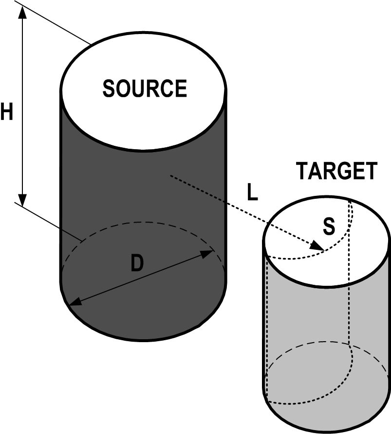
Figure 1: Scheme of the radiation emitted by a solid flame and received by a cilyndrical target (tree).

Finally, $f(\bm{x}_{i}-\bm{x}_{j})$ is estimated considering a view factor between the tree with flames and the target (the neighboring tree) using the concept of solid flame [22]. In this study the source was considered as a cylinder (solid flame) emitting to a target (the neighboring tree) depicted as another cylinder of similar or different dimensions. The radiation can be described using analytical expressions of view factors between a cylinder and a infinitesimal element of surface belonging to the target. A scheme of the set up is shown in Fig. 1. In the most simple scenario we consider the trees as cylinders emitting and absorbing radiation to and from their neighbors. Accordingly to [23], for a cylindrical source and a vertical target, the view factor can be evaluated by:

$$F(H) = \frac{1}{\pi S}\tan^{-1}\left(\frac{h}{\sqrt{S^{2}-1}}\right)-\frac{h}{\pi S}\tan^{-1}\left(\sqrt{\frac{(S-1)}{(S+1)}}\right)+$$ (6)

$$\frac{Ah}{\pi S\sqrt{A^{2}-1}}\tan^{-1}\left(\sqrt{\frac{(A+1)(S-1)}{(A-1)(S+1)}}\right),$$

with:
$A={(h^{2}+S^{2}+1)}/{2S}$, $B={(1+S^{2})}/{2S}$, $S={2L}/{D}$ and $h={2H}/{D}$,
$L$ being the distance between the center of the cylinder to the target, $H$, the height of the cylinder -in the following taken to be about $3\;[m]$- and $D$ -about $2\;[m]$- is the cylinder diameter.

So the total incoming radiation is the integral of the flux factor over the receiving surface $\Sigma$:

$$f(\bm{x}_{i}-\bm{x}_{j})=\int_{\Sigma}\;d^{3}x\;sign(H-z)\;F(\left|H-z\right|)+sign(z)\;F(\left|z\right|)\\$$ (7)

Note that $F(H)$ has been divided in to two contributions, corresponding to the respective portions of flame situated above and below the integration point. It also gives the correct contribution for the case where the point lays higher or lower to the flame.

Using this model we can estimate the radiation received by a punctual target localized at certain distance. Now, as our target is not punctual, but represented by a cylinder it is necessary to integrate over its receiving area. In order to reduce computational time and simplify the model, we assume the simplified surface depicted in Fig. 1. Then, the arc $S$ is a portion of a circle of radius L, thus, orthogonal to the distance. Given this, we only need to calculate the incoming radiation at one point, and colorblack multiplying by the length of the portion of arc S, namely

$$S=2L\left(\pi-2cos^{-1}\left(\frac{r}{2L}\right)\right),$$ (8)

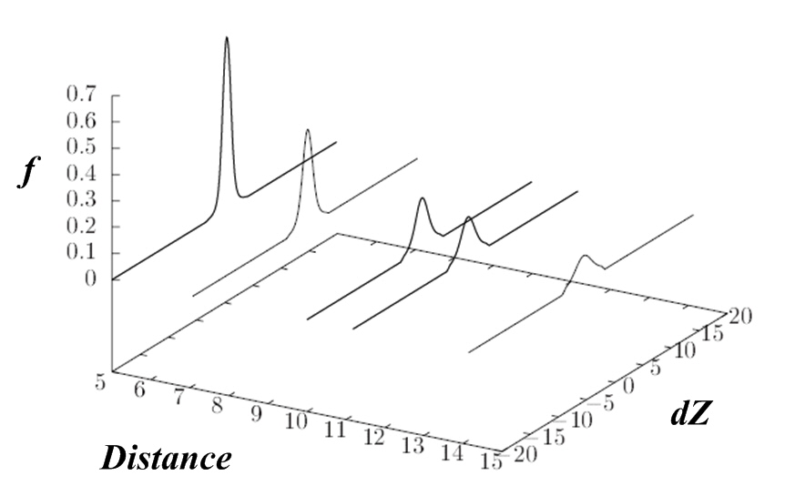
Figure 2: View factors at different distances and heights ($dZ$).

$r$ being the radius of the target ($r\sim 3\;[m]$). Finally we have to integrate along the height of the target to get the total incoming radiation. This last step is done numerically and the resulting radiation at different distances, as function of the difference of height $dz$ is shown in Fig. 2. To incorporate the slope in the description, it is sufficient to change the range of the integral over the receiving canopi, so the height difference between sites is properly reflected.

Finally, to take into account windy scenarios, we will use a reasonable approximation for long distances; The radiation model will be taken to be valid for a thin disc of height $dh$ representing an infinitesimal slice of the flame. Thus, a tilted flame will be composed of several of those discs which energy flux over the neightbours can be estimated as stated before. The flame inclination is calculated as in [27].

Regarding Fig. 2, the quadratic decay will allow us to neglect the interaction between distant neighbors. This will allow us to keep the amount of links between each site relatively small, and conserve the significant long range interactions. This lswn nature can affect largely the percolative properties of the system, for example making the percolation threshold to fall well below the usual values found in first-neighbors systems.

An important final remark has to be done about this factor, as is here where the dependency in the surface is hidden. It relates the flux between two vertical surfaces (cylinders), so it will peak when both are vertically centered. As the surface representing the flame raises above the canopy, it will increase the propagation towards slightly higher surfaces and will produce a decreasing radiative flux for surfaces away from the center. This is the expected behavior and will drive the height dependency in the spreading model.

2.3 Self degradation

Usually, once the decomposition process is started the pyrolysis mass rate is mainly accelerated by the radiation coming from the combustion processes occurring in the tree. Experimentally, this process shows a slow initial evolution if the canopy is ignited while the moisture content is still important. This is followed by an acceleration of the process in the intermediate stage and a new slow down at the end of the process, when the fuel has been mostly consumed. For a burning tree, we propose a mass evolution of the form:

$$\frac{dC_{i}(t)}{dt}=-C_{i}(t)\left(1-C_{i}(t)\right)U_{i},$$ (9)

which is in qualitative concordance with experiments [24]. For large times, $C_{i}(t)$ will decay exponentially, relating the factor $U_{i}$ to the inverse of the mean-life of the isolated burning tree, usually about $30s$ [24].

With this, the overall equation for the rate of mass over time of every active site is:

$$\frac{dC_{i}(t)}{dt}=C_{i}(t)\sum_{<j>}\frac{dC_{j}(t)}{dt}W_{ij}-\Theta\left[C_{i}^{th}-C_{i}(t)\right]C_{i}(t)\left(1-C_{i}(t)\right)U_{i}.$$ (10)

In Eq. 10, the sum over $<j>$ has to be performed over all the burning neighbors of $i$, as we only account for radiative processes. It is important to note that the second term in RHS is activated when the burning threshold $C_{i}^{th}$ is reached, this is controlled by the Heaviside $\Theta$ step function.

3 Numerical tests

The system here described can be solved numerically with relative ease. Following we study two different scenarios to get an insight of the behavior of the model. First we will see a small system of only 4 trees, where we will be able to analyze quantitatively the behavior of the model and the evolution of $C_{i}(t)$ for a burning system. Later we go to a larger system, in order to study the percolation like properties and its critical behavior.

In the following we will consider a mean life of a burning tree to be $30\;[s]$, the degradation coefficient $\alpha=0.000005\;[J^{-1}]$, the burning threshold $C_{i}^{th}=0.9$, and the heat of combustion $c_{h}=12000\;[kJ/kg]$.

3.1 Four sites evolution

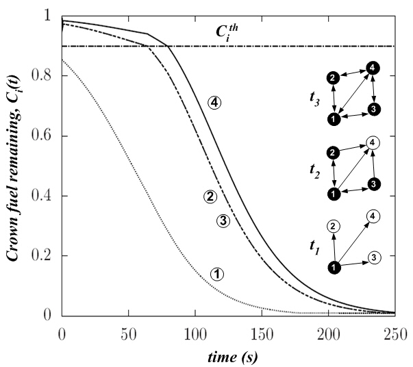
Figure 3: Simple interaction example of four trees in and flat landscape. The curves shows the fuel available in each site in function of time and the schematic inside the graph represent the interaction at different times.

Once the parameters discussed in the previous section are fixed and the numerical simulation is implemented, it is interesting to look the simple interaction between four trees symmetrically distributed (see the schematics in the Fig. 3). The simulation was started burning only site 1. At $t_{1}$ only the site 1 release energy causing the degradation of the site 2, 3 and 4. Once the threshold of ignition $C_{th}$ is reached at $t_{2}$, both sites 2 and 3 are ignited simultaneously. The evolution for the sites 2 and 3 are identical due to the symmetry and only three curves are observed in the graph. Regarding the evolution of each curve, there is an evident change in the slope when any of them reaches the ignition threshold $C_{th}$. At $t_{3}$ the site 4 is burning and the self burning process accelerates the degradation. Clearly these processes of self-burning contributes to increase the slope for the fuel mass losses evolutions of the neighboring trees. For larger times, the mass decays exponentially and as its derivative also goes to zero, the effect on the neighbors also decreases. Finally, it is important to note that the evolution of the fuel reaming in the tree along the time, exhibits the typical behavior observed in experimental results [24].

3.2 Front evolution

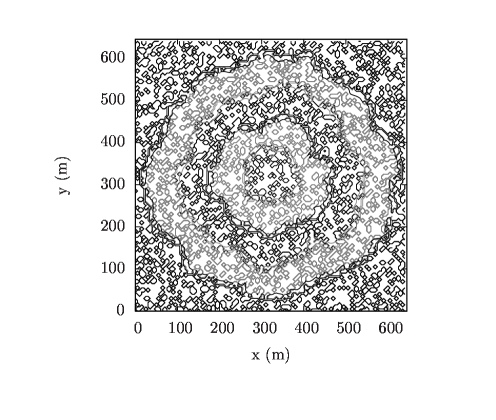
(a)

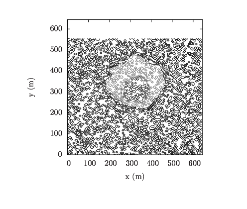
(b)

Figure 4: (a)Evolution of the fire front ignited in the middle of the mesh, in a flat surface without slope and a dopping of $80\%$. (b)In this case the surface has an inclination of $\pi/6\;[rad]$. The alternated black and gray patterns represents the evolution of the system with a time difference of 10 minutes.

We now illustrate the spreading of fire through a bigger domain. We use a square mesh of 129 sites per side, with a separation of 10 $[m]$ between each site. In Fig. 4 we show the time evolution of the fire front in a flat surface with no slope and other with an inclination of $\pi/6\;[rad]$, both with an occupancy of the $80\%$. The state of the system is obtained at different times, separated by intervals of approximately $5$ minutes.

The simulations produce fire patterns accordingly to the expected behavior, climbing faster up hill and with just small effects of the underlying square mesh.

3.3 Critical Behavior

The last important point we will investigate, is the analysis of the second order phase transition usually found in this kind of systems. As before, the fire was simulated over a square lattice, using a simple scenario of a flat surface with different inclinations, ranging from $0$ to $\pi/3$, keeping the total distance between neighboring sites fixed at $5\;[m]$ as before. The runs starts with a single site as a seed in the center of the mesh and are stopped when the fire front reaches the borders of the domain or when the propagation of the fire is stopped. In this way the finite size effects are irrelevant. To keep the simulations as simple as possible, we choose the neighborhood to be the eight closest sites to each active site. In this way the blocking effects are unimportant and we can focus on the features of the spreading model (see Eq. 10).

Although simple, the network spawned in this way brings some theoretical complications, as we are no longer dealing with a simple symmetric network, due to the weighting procedure explained in the previous sections. For the low slope case, this will not be important, but as the inclination grows this effect will be apparent and will not allow us to use some of the usual constructs. In the following we will try to keep the discussion in the more general way we can, avoiding the use of quantities not always well defined.

To study criticality, we measure the survival probability $P_{s}(t)$, the number of active sites $N(t)$ and the mean square radius, $R^{2}(t)$, of the infected zone starting from the ignition point. Those quantities are averaged over all surviving runs. The literature shows that in this case it is reasonable to expect a behavior at the critical point as [25]:

$$P_{s}(t)\sim t^{-\delta},\;N(t)\sim t^{\theta},\;R^{2}(t)\sim t^{2/z}$$ (11)

The dynamical study of the critical behavior best suits this particular configuration, since other quantities like correlation length or cluster size loses their meaning in a non symmetric network, as mentioned before.

In Fig. 5a the percolation probability $\theta(p)$, for the different slopes is shown. Low inclinations in the burning surface produces roughly constant percolation thresholds, reaching a peak close to $0.8\;[rad]$ from where it decreases almost linearly for higher slopes, as shown in Fig. 5b.

At criticality, $N$ and $R^{2}$ are plotted in Fig. 6a and Fig. 6b respectively. Both quantities colorblack show a power law behavior at large times. The different inclinations, depicted in different lines, produce different critical behaviors. In both cases the critical exponent increases with the slope, thus showing faster and more active fire spreads, as expected. For $N$ we have that $\theta$ ranges from $1.173$ to approximately $1.996$, whereas for $R^{2}$, ${2}/{z}$ has a minimum at about $1.705$ to a maximum of $2.098$. Those ranges comprehend the values reported in [26] for the General Epidemic Process (GEP) in a two dimensional lattice.

4 Experimental Validation

In this last section we will compare our model to a forest fire ignited near Lançon in Provence, France, at 9:40 on July the first of 2005. There were reported two ignition points and the mean wind speed reached $46\;[km/h]$ at $10\;[m]$ avobe the ground, with an average wind direction of about $330\deg$ (NNW).

The main vegetation type present in the fire is the kermes oak shrubs (Quercus coccifera), for which we use a mean life of $17\;[s]$ and a radiation constant $\alpha=4.2\;10^{-6}\;[J^{-1}]$. The vegetation and terrain data is available at a resolution of $50\;[m]$, so for the terrain we use a bilinear interpolation and for the vegetation, the $50\;[m]$ sided cell is filled with kermes oaks at a distance of $3.7\;[m]$ with an ocupancy probability of $0.64$. For more details of this scenario see e.g. Ref.[28].

Data of the fire front advance is available at 12:00 and 14:34 hrs. In table 1 we present the burned area and the rate of spread (ROS) of the fire and the simulation results, and in Figure 7 an aerial comparisson of the numerical results versus the data.

	Time	Fire	Simulation
ros (m/h)	12:00	714	1
	14:34	1523	1
Burned Surface (ha)	12:00	148	1
	14:34	485	1

Table 1: Rate of spread and burned surface for the fire of Lançon and simulation.

The burned area is slightly overestimated. Part of this discrepancy can be explained by the action of firefighters starting around 13:00 hrs. The model gives a reasonable description of the fire pattern, inspite of the roughness of the radiative model and the physical description of the vegetation content. Work in this respect is being carried out [29] and we envisage a future improvement on those areas. None the less, the propagation model 10 shows the relevant features one expects and seems to be adecuate for real-life scenarios.

5 Conclusions

We have developed and tested a new continuous model for the fire spread under the $lswn$ approach. The model is controlled by a phenomenological dynamics and is able to reproduce realistic spreading scenarios. It allows including heterogeneous vegetation (type, geometry, mass, etc.), as well as changes in the topography, this latter characteristic being one of interest in the present work. The heterogeneity of the landscape is captured via geometric factors included locally in each site as parameters of the dynamic equations. This gives a simple starting point to future studies where more effects will be included. For example, the wind effects can be introduced in the description modifying only the geometric factors between each site.

In the present study, the model was used to simulate the fire spreading process in different landscapes for a defined kind of vegetation. First, it was shown that the fire spread exhibits–as the classical percolation picture–a continuous phase transition between a self-extinguishing state and an infinite spreading one, depending on the occupancy probability $p$. Secondly, it was observed that for surfaces with constant slope, the percolation threshold shows an increasing behavior with the inclination, which produces greater critical exponents for inclined configurations.

We plan the introduction in this model of a more complete description of the sites network, including for example an amorphous mesh over a fractal landscape and where the blocking of trees are fully taken into account.

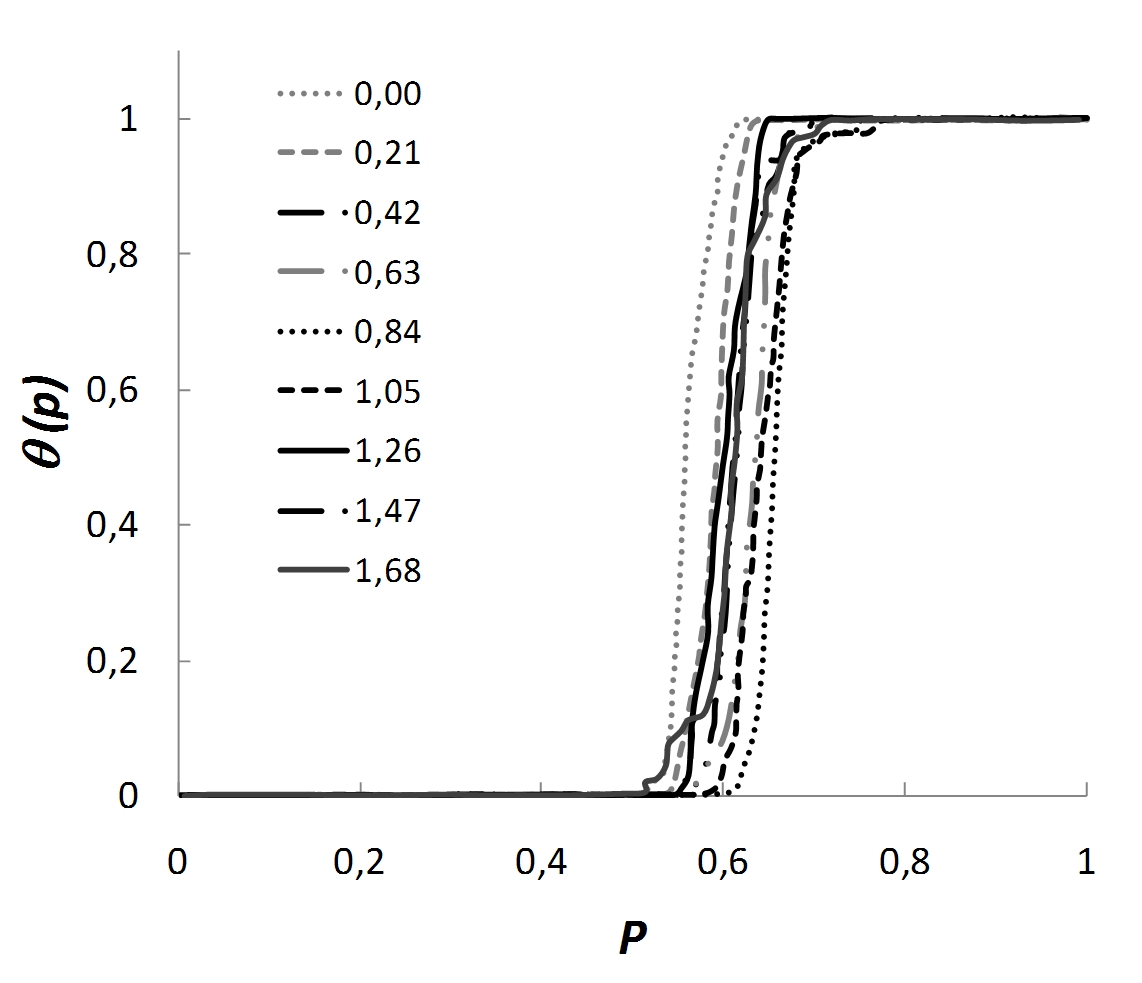
(a)

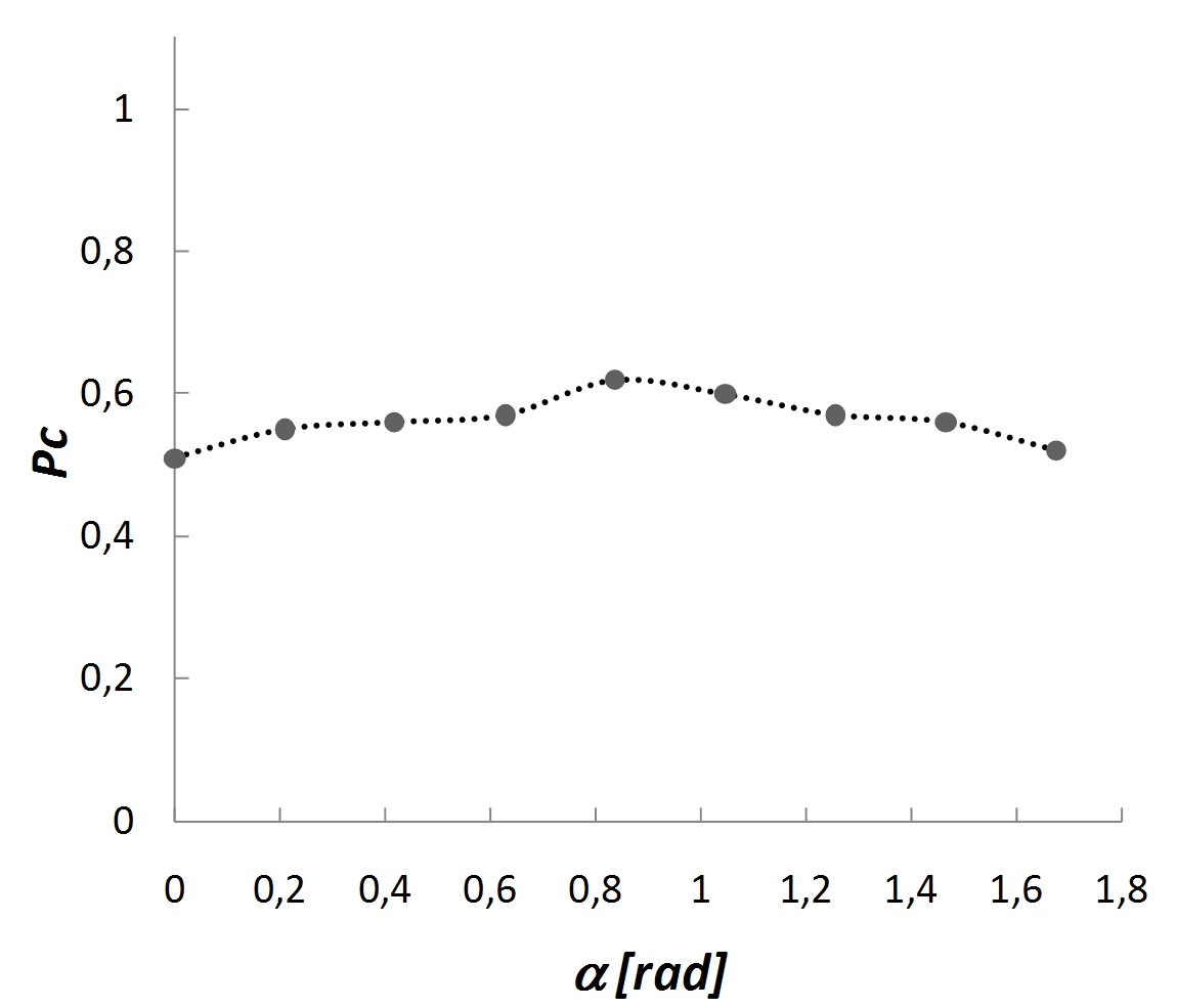
(b)

Figure 5: (a) The percolation density for different inclinations. (b) The percolation threshold as function of the slope.

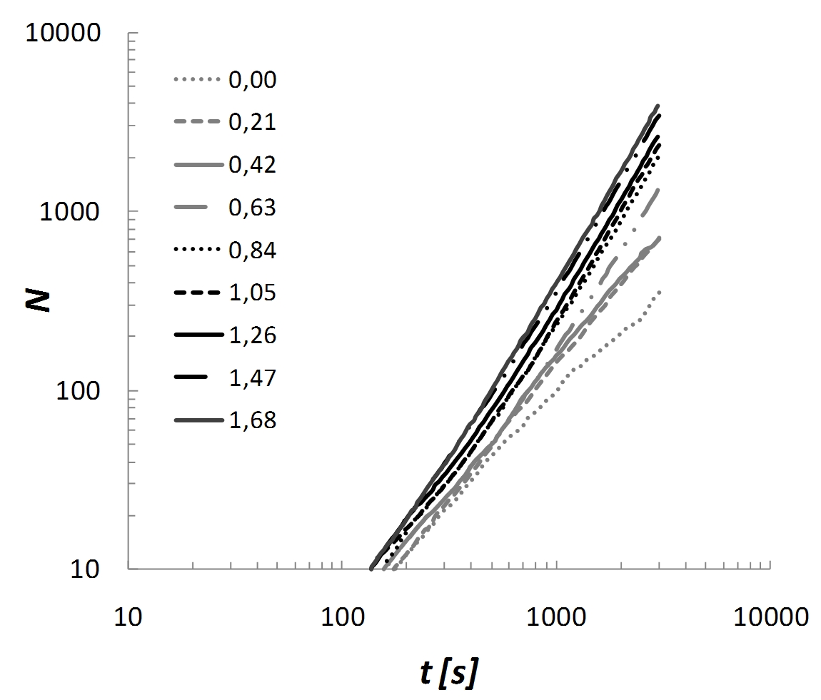
(a)

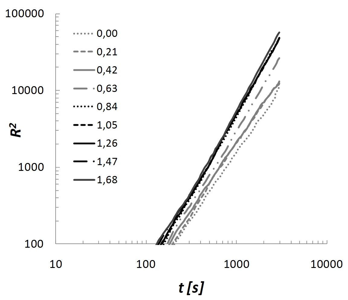
(b)

Figure 6: (a) The number of active sites $N(t)$. (b) The mean square radius R². Both results were obtained at criticality for different slopes $\alpha$.

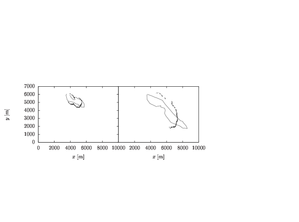
Figure 7: Fire front contours for the fire of Lançon. The lines delimit the actual burned area, the points represent the simulated fire front.

References

- [1] R.O. Weber, Prog. Energy Combust. Sci. 17 (1982) 67–82.
- [2] A.G. McArthur, Forest Research Institute, Australian Forest and Timber Bureau Leaflet (1966) 100.
- [3] R.C. Rothermel, A Mathematical Model for Predicting Fire Spread in Wildland Fuels. USDA Forest Service, Intermountain Forest and Range Experiment Station General Technical Report INT-11, 1972.
- [4] W. Mell, M.A. Jenkins, J. Gould, P. Cheney, Int. J. Wildland Fire 16 (2007) 1–22.
- [5] R. Linn, J. Reisner, J.J. Colman, J. Winterkamp, Int. J. Wildland Fire 11 (2002) 233-246.
- [6] O. Sero-Guillaume, J. Margerit, Int. J. Heat and Mass Transfer 45 (2002) 1705–1722.
- [7] D. Morvan, J.L. Dupuy, Combust. Flame 127 (2001) 1981–1984.
- [8] A.P. Dimitrakopoulos, R.E. Martin, Concepts for future large fire modeling. In: Proceedings of the Symposium on Wildland Fire 2000, South Lake Tahoe, Calif., 1987, 27-30.
- [9] G. Caldarelli, R. Frondoni, A. Gabrielli, M. Montuori, Europhys. Lett. 56 (2001) 510–516.
- [10] G. Albinet, G. Searby, and D. Stauffer, J. Phys. 47 (1986) 1–8.
- [11] H. Téphany, J. Nahmias, and J.A.M.S. Duarte, Physica A 242 (1997) 57–69.
- [12] G.L. Ball and D.P. Guertin, Int. J. Wildland Fire 2 (1992) 47–54.
- [13] F.J. Barros and M.T. Mendes, Simul. Practice Theory 5 (1997) 185–197.
- [14] P.G. de Gennes, La Recherche 7 (1976) 919.
- [15] M.E.J. Newman, I. Jensen, R.M. Ziff, Phys. Rev. E 65 (2002) 021904.
- [16] B. Porterie, N. Zekri, J.-P. Clerc, J.-C. Loraud, Combust. Flame 149 (2007) 63–78.
- [17] N. Zekri, B. Porterie, J.P. Clerc, J.C. Loraud, Phys. Rev. E 71 (2005) 046121 .
- [18] D.J. Watts, S.H. Strogatz, Nature 393 (1998) 440.
- [19] B. Porterie, A. Kaiss, J.P. Clerc, N. Zekri, L Zekri, arXiv:0805.3365v1 [physics.soc-ph]
- [20] M.E.J. Newman, D.J. Watts, Phys. Lett. A 263 (1999) 341–346 .
- [21] I. Atreya, Phil. Trans. R. Soc. Lond. A 356 (1998) 2787–2813.
- [22] A.L. Sullivan, P.F. Ellis, I.K. Knight, Int. J. Wildland Fire 12 (2003) 101–110.
- [23] M. Shokri, C.L. Beyler, SFPE Journal of Fire Protection Engineering 4 (1989) 141–150.
- [24] W. Mell, A. Maranghides, R. McDermott, S.L. Manzello, Combust. Flame 156 (2009) 2023–2041.
- [25] S.M. Dammer, H. Hinrichsen, Phys. Rev. E (2003) 68 016114.
- [26] F. Linder, J. Tran-Gia, S.R. Dahmen, H. Hinrichsen, arXiv:0802.1028v1 [cond-mat.stat-mech]
- [27] F.A.Albini, A model for the wind blown flame from a line fire, Combust. Flame 43 (1981) 155–174.
- [28] J.K. Adou, Y. Billaud, D.A. Brou, J.-P. Clerc, J.-L. Consalvi, A. Fuentes, A. Kaiss, F. Nmira, B. Porterie, L. Zekri and N. Zekri, Ecological Modelling 221 (2010) 1463–1471
- [29] Y. Billaud, A. Kaiss, J.L. Consalvi, B. Porterie, “Monte Carlo Estimation of Thermal Radiation from Wildland fires”, Journal of Thermal Science, submitted