The Schwinger model with $N_{f}\geq 2$ flavors is a simple example for a fermionic model with zero chiral condensate $\Sigma$ (in the chiral limit). We consider numerical data for two light flavors, based on simulations with dynamical chiral lattice fermions. We test properties and predictions that were put forward in the recent literature for models with $\Sigma=0$, which include IR conformal theories. In particular we probe the decorrelation of low lying Dirac eigenvalues, and we discuss the mass anomalous dimension and its IR extrapolation. Here we encounter subtleties, which may urge caution with analogous efforts in other models, such as multi-flavor QCD.

1 Chiral symmetry and the microscopic
Dirac spectrum

Chiral symmetry plays a key rôle in our understanding of systems with light fermions. The chiral condensate $\Sigma=-\langle\bar{\Psi}\Psi\rangle$ is the order parameter, which indicates whether this symmetry is intact ($\Sigma=0$) or broken ($\Sigma>0$). The latter is generic at finite fermion mass $m$, but in the chiral limit $m\to 0$ both scenarios occur, depending on the model and its parameters:

$\bullet$ $\Sigma(m\to 0)>0$ is the familiar situation in QCD at low temperature, where the $SU(N_{f})_{L}\otimes SU(N_{f})_{R}$ chiral flavor symmetry breaks spontaneously down to $SU(N_{f})_{L+R}$. In our world we encounter 2 (or 3) light quark flavors and quasi-spontaneous chiral symmetry breaking. This gives rise to 2 (or 8) light pseudo-Nambu-Goldstone bosons, which are identified with light mesons.

In 2 dimensions, spontaneous symmetry breaking can only occur for discrete symmetries, as we know from the Mermin-Wagner Theorem [1]. Nevertheless the $N_{f}=1$ Schwinger model [2] (Quantum Electrodynamics in 2 space-time dimensions) belongs to this class as well, although its chiral symmetry is continuous; in this case it breaks explicitly, even at $m=0$, due to the axial anomaly. The value $\Sigma(m\to 0)\simeq 0.160\,g$ was predicted theoretically [2], and confirmed numerically [3] ($g$ is the gauge coupling).

$\bullet$ The opposite scenario, with $\Sigma(m\to 0)\to 0$, has recently attracted considerable interest, in particular because it includes the IR conformal theories. A vanishing chiral condensate is generally expected at high temperature, in particular for QCD above the chiral crossover, which seems to coincide with the deconfinement phase. It also encompasses the quenched approximation, and $SU(2)$ gauge fields [4].

At low temperature, multi-flavor QCD — in particular the extension of QCD to $N_{f}=8$ or $12$ light flavors — is currently a subject of intensive research [5, 6, 7, 8, 10]. The question whether or not IR conformality emerges — resp. above which number $N_{f}$ this happens — is today one of the most controversial issues in the lattice community. In particular, for $N_{f}=12$ evidence has been reported both for [6, 7, 10] and against [8] this property. A prominent motivation is the search for nearly conformal gauge theories, where the coupling moves only little (“walks”) in some energy regime, as reviewed in Ref. [11]. That property is of interest in the framework of the ongoing attempts to revitalize technicolor approaches.

As a further example of the second scenario, we are going to address the $N_{f}=2$ Schwinger model. Its Lagrangian in a continuous Euclidean plane reads

$${\cal L}(\bar{\Psi},\Psi,A_{\mu})=\frac{1}{2}F_{\mu\nu}F_{\mu\nu}+$$

$$(\bar{\Psi}^{(1)},\bar{\Psi}^{(2)})\left(\begin{array}[]{cc}\gamma_{\mu}({\rm i}\partial_{\mu}+gA_{\mu})+m&0\\ 0&\gamma_{\mu}({\rm i}\partial_{\mu}+gA_{\mu})+m\end{array}\right)\left(\begin{array}[]{c}\Psi^{(1)}\\ \Psi^{(2)}\end{array}\right)\ .\ \qquad$$ (1.5)

$A_{\mu}(x)$ is an Abelian gauge field $(\mu=1,2)$, and $F_{\mu\nu}$ is the corresponding field strength tensor. $\gamma_{\mu}$ are Euclidean Dirac matrices; we can represent them by two Pauli matrices. The fermions are given by a 2-component spinor field $\Psi^{i}(x)$ for each flavor. Here we consider two flavors with degenerate mass $m$. It can be incorporated in the Lagrangian without breaking gauge symmetry, since this is a “vector theory”, where both flavors couple to the gauge field in the same way (in contrast to “chiral gauge theories”, such as the electroweak sector of the Standard Model).

For the lattice gauge field we use the standard formulation in terms of compact link variable $U_{x,\mu}\in U(1)$ (where $x$ is a lattice site), see e.g. Refs. [12]. The Grassmann functional integral over the fermion fields yields the determinant of the Dirac operator, which the Hybrid Monte Carlo algorithm deals with [12]. We will comment on the lattice Dirac operator in Section 2.

In this case the coupling $g$ is energy independent, and $N_{f}\geq 2$ is sufficient to attain $\Sigma(m\to 0)\to 0$, as we see from the relation [13]

$$\Sigma(m)\propto m^{1/\delta}\ ,\qquad\delta=\frac{N_{f}+1}{N_{f}-1}\ ,$$ (1.6)

which holds in infinite volume, $V=\infty$. In a finite volume $V=L\times L$ — or when taking the chiral limit and the infinite volume limit simultaneously — the critical exponent $\delta$ depends on the dimensionless Hetrick-Hosotani-Iso parameter [14]

$$l=\frac{m}{\pi^{1/4}}\ \sqrt{2L^{3}g}\ .$$ (1.7)

Eq. (1.6) holds for $l\gg 1$, whereas the opposite extreme, $l\ll 1\ll 2Lg/\sqrt{\pi}\,$, leads to $\delta=1$ (which corresponds to the free fermion [15]).

The chiral condensate is related to the density $\rho(\lambda)$ of Dirac eigenvalues $\lambda$ at zero by the Banks-Casher relation [16],

$$\frac{1}{\pi}\,\Sigma(m=0)\ =\ ^{\lim}_{\lambda\to 0}\ {}^{\lim}_{m\to 0}\ {}^{\lim}_{V\to\infty}\ \rho(\lambda)$$ (1.8)

(the order of the limits is specified e.g. in Ref. [17]). In finite volume, the scenario of a finite $\Sigma$ implies a plateau of the spectral density $\rho$ near $\lambda=0$. In the $\epsilon$-regime of QCD, i.e. in a small 4d box, the prediction for $\rho(\lambda)$ has been refined by Random Matrix Theory [18]. The corresponding wiggle structure on top of the Banks-Casher plateau agrees with lattice data for staggered fermions [19] and for overlap fermions [20, 21]; the latter also capture correctly the dependence on the topological sector.

A behavior that corresponds to the $\Sigma=0$ scenario — and therefore to the absence of a Banks-Casher plateau — is a power-law for the low-lying Dirac eigenvalue density with some exponent $\alpha$,

$$\rho(\lambda)=c\,V\,|\lambda|^{\alpha}\ ,$$ (1.9)

where $c$ is a constant. In fact, it is natural to expect $\alpha$ to coincide with the inverse critical exponent $\delta$, i.e. $\Sigma(m)\propto m^{\alpha}$ [22].

In the case of high temperature — i.e. a short extent in Euclidean time — the factor $V$ in eq. (1.9) represents the spatial volume, since small non-zero Dirac eigenvalues only occur in spatial directions. This is the scenario studied by T.G. Kovács in Ref. [4]. He postulated for this setting the absence of correlations between the Dirac eigenvalues, i.e. a Poisson-type statistics. Thus he assumed the distribution of small eigenvalues in two disjoint intervals to be independent (unlike the Random Matrix behavior). With the additional assumption (1.9), he derived the first eigenvalue density (for $m=0$) as [4]

$$\rho_{1}(\lambda)=cV\lambda^{\alpha}\,\exp\Big{(}-\frac{cV}{\alpha+1}\lambda^{\alpha+1}\Big{)}\ .$$ (1.10)

Kovács proceeded from $\rho_{1}(\lambda)$ to $\rho_{2}(\lambda)$ by an integral over the product of the probabilities for having a first eigenvalue at $\lambda_{1}$, another one at $\lambda>\lambda_{1}$, and no eigenvalue in between. By iterating this step we obtain

$$\rho_{n}(\lambda) = \int_{0}^{\lambda}d\lambda^{\prime}\ \rho_{n-1}(\lambda^{\prime})\,P_{\rm no\,EV}(\lambda^{\prime},\lambda)\,\rho(\lambda)$$ (1.11)

$$= \frac{1}{(n-1)!}\frac{(cV)^{n}}{(\alpha+1)^{n-1}}\lambda^{n(\alpha+1)-1}\exp\Big{(}-\frac{cV}{\alpha+1}\lambda^{\alpha+1}\Big{)}\ ,$$

where the probability for no eigenvalue in some interval $[\lambda_{a},\lambda_{b}]$ is given by

$$P_{\rm no\,EV}(\lambda_{a},\lambda_{b})=\exp\Big{(}\frac{cV}{\alpha+1}(\lambda_{a}^{\alpha+1}-\lambda_{b}^{\alpha+1})\Big{)}\ .$$ (1.12)

2 Simulations of the 2-flavor Schwinger
model with chiral fermions

We are going to confront this prediction with data obtained in simulations of the $N_{f}=2$ Schwinger model, with dynamical overlap hypercube fermions [23, 21]. The latter is a variant of a Ginsparg-Wilson fermion, where the lattice Dirac operator is constructed by inserting a truncated perfect hypercube lattice Dirac operator $D_{\rm HF}$ into the overlap formula [24],

$$D_{\rm ovHF}(m) = \Big{(}1-\frac{m}{2}\Big{)}D_{\rm ovHF}(0)+m\ ,$$

$$D_{\rm ovHF}(0) = 1+(D_{\rm HF}-1)/\sqrt{D^{2}_{\rm HF}-1}\ .$$ (2.1)

This provides exact (lattice modified) chiral symmetry [25] at $m=0$, along with an excellent level of scaling and locality, as well as approximate rotation symmetry [23]. All these properties are far superior to the standard overlap operator. They are based on the similarity between the (renormalization group improved) kernel and the chiral operator, $D_{\rm HF}\approx D_{\rm ovHF}$. Regarding the simulation with a Hybrid Monte Carlo algorithm, that similarity enables in addition the use of a simplified force term [26].

The simulations were carried out at $\beta=1/g^{2}=5$, which leads to plaquette values close to $0.9\,$. Hence we are dealing with fine lattices, and a continuum extrapolation is not essential. The volumes have the shape $L\times L$ with $L=16\dots 32$, and we consider the light fermion masses $m=0.01$ and $0.06$. Depending on these parameters, finite size effects may be significant.

We analyze eigenvalues $\lambda_{n}$ of the operator $D_{\rm ovHF}(0)$, after mapping them from the unit circle in the complex plane (with center and radius 1) onto ${\kern 2.5pt\sf{R}\kern-7.79999pt\sf{I}\kern 7.79999pt\kern-2.5pt}_{+}\,$, by means of the Möbius transform

$$\lambda_{n}\to\left|\frac{\lambda_{n}}{1-\lambda_{n}/2}\right|\ .$$ (2.2)

As a generic property, the density of small Dirac eigenvalues depends on the topological sector, which can be defined by identifying the fermion index $\nu$ with the topological charge [27].

In a previous consideration with fits to the detailed distributions of $\lambda_{1}$, $\lambda_{2}$, $\lambda_{3}$ (and $\lambda_{4}$), we obtained good agreement with the exponent $\alpha=3/5$, in particular in the topologically neutral sector ($\nu=0$) [26]. On the other hand, in infinite volume one expects $\alpha=1/3\,$, based on eq. (1.6). This discrepancy becomes plausible if we consider the Hetrick-Hosotani-Iso parameter $l$ of eq. (1.7). In Table 1 we display the values of $l$ in our smallest and largest volume.

	$L=16$	$L=32$
$m=0.01$	$0.455$	$1.286$
$m=0.06$	$2.728$	$7.715$

Table 1: The values of the Hetrick-Hosotani-Iso parameter $l$ (defined in eq. (1.7)), for the two fermion masses $m$, and the extreme lattices sizes $L$, which we consider in this work.

3 Testing the decorrelation of the low-lying Dirac eigenvalues

We could test Kovács’ conjecture for the model under consideration by comparing the functions (1.11) to histograms. However, in order to avoid the arbitrary choice of a bin size, we prefer to compare the corresponding cumulative densities,

$$R_{n}(\lambda)=\int_{0}^{\lambda}d\lambda^{\prime}\,\rho_{n}(\lambda^{\prime})=1-\exp\Big{(}-\frac{cV}{\alpha+1}\lambda^{\alpha+1}\Big{)}\ \sum_{k=0}^{n-1}\frac{1}{k!}\ \Big{(}\frac{cV}{\alpha+1}\lambda^{\alpha+1}\Big{)}^{k}\ .\$$ (3.1)

Treating the constants $\alpha$ and $c$ as free parameters, we illustrate in Figure 1 the fits of $R_{n}(\lambda)$ to our data at $m=0.01$ and $L=16,\ 20$ and $32$, in the topologically neutral sector ($\nu=0$).

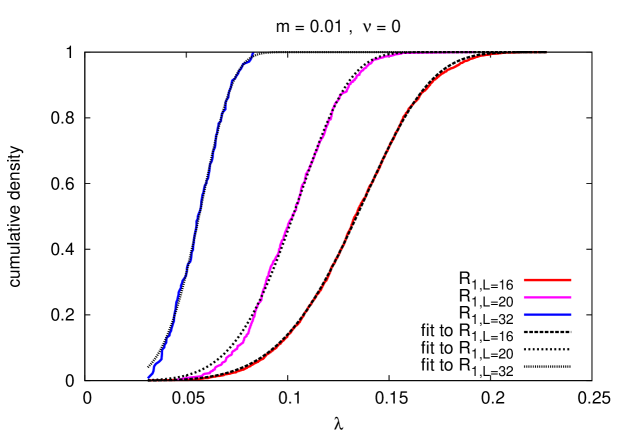
Figure 1: The cumulative density of the first Dirac eigenvalue of the massless operator $D_{\rm ovHF}(0)$, based on configurations generated at fermion mass $m=0.01$ and topological charge $\nu=0$, on lattices of size $L=16$, $20$ and $32$. In all cases, there is excellent agreement between the data and fits to the function $R_{1}(\lambda)$ in eq. (3.1), with adjusted parameters $\alpha$ and $c$.

Excellent fits are also achieved if we consider higher eigenvalues, as Figure 2 shows for $R_{n}$, $n=1,2,3$, at $m=0.01$, $L=16$, in the sectors $|\nu|=0$ and $1$.

In order to quantify this agreement, Table 2 gives results of Kolmogorov-Smirnov (KS) test, which compares numerical data for a cumulative density with a theoretical prediction, see e.g. Ref. [28]. The KS index is between 0 (extreme disagreement) and 1 (perfect congruousness), and experience shows that a KS index $\gtrsim 0.5$ characterizes a manifestly good agreement. (The low value for $L=16$, $\nu=0$, $\lambda_{3}$ appears surprising since the data are not too far from the theoretical curve. However, even the impact of small deviations is large in this case due to the high statistics of 2428 configurations.)

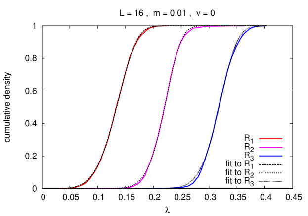
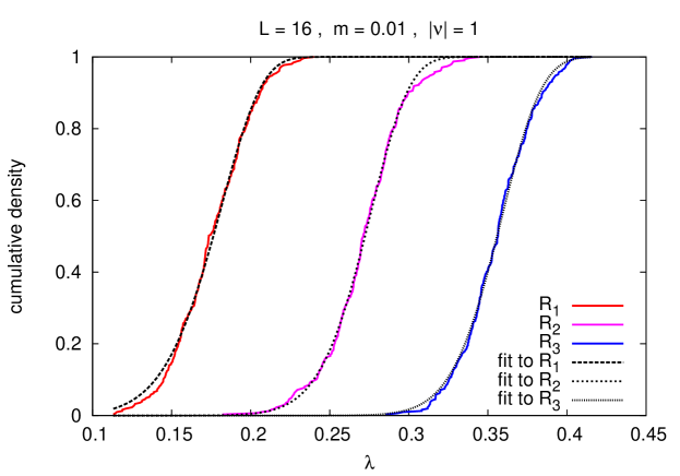
Figure 2: Cumulative densities for the first three Dirac eigenvalues, at $L=16$ and $\nu=0$ (above), $|\nu|=1$ (below). In each case, tuning $\alpha$ and $c$ leads to good agreement with the functions $R_{n}(\lambda)$, $n=1,2,3$, in eq. (3.1). However, the required parameter values are not consistent, see Table 3.

$L$	$|\nu|$	eigenvalue	Kolmogorov-Smirnov index
16	0	$\lambda_{1}$	0.748
20	0	$\lambda_{1}$	0.517
32	0	$\lambda_{1}$	0.962
16	0	$\lambda_{2}$	0.648
16	0	$\lambda_{3}$	0.013
16	1	$\lambda_{1}$	0.567
16	1	$\lambda_{2}$	0.727
16	1	$\lambda_{3}$	0.693

Table 2: The Kolmogorov-Smirnov confidence index for the cumulative eigenvalue densities in Figures 1 and 2, compared with the functions $R_{n}(\lambda)$ in eq. (3.1), with the optimal parameters $\alpha$ and $c$, which are used for the curves in the plots and displayed in Table 3.

$L$	$|\nu|$	$n=1$		$n=2$		$n=3$
		$\alpha$	$c/1000$	$\alpha$	$c/1000$	$\alpha$	$c/1000$
16	0	4.199(3)	0.486(3)	5.836(5)	$1.40(1)$	6.16(1)	0.274(4)
16	1	7.08(5)	$27(2)$	8.08(5)	$8.0(6)$	8.45(6)	$1.7(1)$
20	0	4.23(2)	$1.35(7)$	6.00(2)	9.0(3)	6.56(3)	2.6(1)
32	0	3.75(3)	$2.8(3)$	5.02(7)	14(3)	5.4(1)	6(2)

Table 3: The parameters $\alpha$ and $c$ (the latter in units of $10^{3}$), obtained by fitting formula (3.1) to our data at $m=0.01$ for the cumulative densities of $\lambda_{n}$, $n=1,2,3$.

The corresponding parameters are given in Table 3. They create first doubt about the confirmation of the decorrelation property: for fixed $m$, $L$ and $\nu$, the fitting parameters $c$ and $\alpha$ are not quite consistent for $R_{1}$, $R_{2}$ and $R_{3}$. Of primary interest is the (dimensionless) exponent $\alpha$; its fluctuation is relatively mild, but all fitted values deviate strongly from $\alpha=3/5$, the value which was determined directly from the distributions of these eigenvalues [26].

Before we continue with the interpretation, we also consider the mean eigenvalues. Formula (1.11) predicts them in terms of $\Gamma$-functions,

$$\langle\lambda_{n}\rangle=\int_{0}^{\infty}d\lambda\ \rho_{n}(\lambda)\,\lambda=\frac{1}{(n-1)!}\Big{(}\frac{\alpha+1}{cV}\Big{)}^{1/(\alpha+1)}\Gamma\Big{(}n+\frac{1}{\alpha+1}\Big{)}\ .$$ (3.2)

The corresponding numerical results are given in Table 4.

$L$	$|\nu|$	$\langle\lambda_{1}\rangle$	$\langle\lambda_{2}\rangle$	$\langle\lambda_{3}\rangle$	$\langle\lambda_{4}\rangle$
16	0	0.1328(6)	0.219(1)	0.3180(6)	0.3858(5)
16	1	0.175(2)	0.271(2)	0.355(3)	0.423(1)
20	0	0.102(2)	0.164(2)	0.238(1)	0.294(1)
20	1	0.127(3)	0.202(3)	0.268(2)	0.322(1)
28	1	0.082(3)	0.132(3)	0.176(4)	0.213(2)
32	0	0.056(3)	0.095(4)	0.133(4)	0.165(4)
32	1	0.076(3)	0.109(1)	0.153(3)	0.181(3)

Table 4: The mean values of the first four eigenvalues of the massless Dirac operator, in distinct topological sectors, for configurations generated at $m=0.01$.

If we focus on $\langle\lambda_{1}\rangle$, for instance at $m=0.01$, $|\nu|=1$ and $V=16^{2}$, $20^{2}$, $28^{2}$ and $32^{2}$, we obtain again a decent fit, see Figure 3 (bold line). This is not that conclusive, but not trivial either for four volumes and two free parameters.

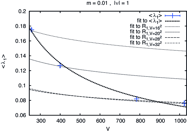
Figure 3: Fits of the function in eq. (3.2) to our data for $\langle\lambda_{1}\rangle$, at $|\nu|=1$, in volumes $V=16^{2},\ 20^{2},\ 28^{2},\ 32^{2}$, with the parameters of Table 5 (bold line). For comparison we show the curves that correspond to the parameters of Table 3, which are fixed for the densities of the $\lambda_{1}$ data in separate volumes.

These fits become highly non-trivial if we extend the consideration to $\langle\lambda_{n}\rangle$ for $n=1\dots 4$, and require a unique set of parameters for each topological sector. The data in the sector $|\nu|=1$ (where we have results in four volumes) can be fitted well, see Figure 4. The corresponding parameters are given in Table 5; they are compatible with the value $\alpha=3/5$, which matches well the detailed distributions of the leading 3 (or 4) eigenvalues [26], as we mentioned in Section 2.

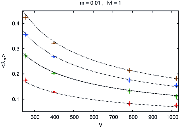
Figure 4: Mean values of the leading $D_{\rm ovHF}(0)$ eigenvalues $\langle\lambda_{1}\rangle\dots\langle\lambda_{4}\rangle$ for data obtained at $m=0.01$ and $L=16\dots 32$. We use one set of fitting parameters $\alpha$ and $c$ for $|\nu|=1$. The four eigenvalues are captured well. However, the parameter values — given in Table 5 — are incompatible with those of the fits in Figures 1 and 2 (given in Table 3).

$|\nu|$	$\alpha$	$c$
0	0.63(3)	0.13(1)
1	0.58(3)	0.09(3)

Table 5: The parameters $\alpha$ and $c$ obtained by fitting the mean eigenvalues $\langle\lambda_{1}\rangle\dots\langle\lambda_{4}\rangle$, at $m=0.01$, in boxes of size $L=16\dots 32$ (cf. Figure 4).

If we compare again the required values of $\alpha$ and $c$ for these fits, we see that they differ by orders of magnitudes from those obtained from the cumulative densities, cf. Table 3. This is not a contradiction; if we compare the latter values with $\langle\lambda_{i}\rangle$ in each single case, it works as well, as we see from the four finer lines in Figure 3. However, once we fix these values, we cannot capture several volumes.

As a final aspect in this context, we consider the unfolded level spacing density. One numerates the Dirac eigenvalues of each configuration separately in ascending order, puts them all together and numerates again. The spacing in this global order between eigenvalues, which are adjacent in the ordering of one configuration — divided by the number of configurations — is the unfolded level spacing $s$. We have shown in Ref. [26] that the total spectrum follows the statistical distribution of the Chiral Unitary Ensemble [29] (also known as the $\beta=2$ Wigner-Dyson form),

$$\rho_{\chi{\rm UE}}(s)=\frac{32s^{2}}{\pi^{2}}\exp(-4s^{2}/\pi)\ ,$$ (3.3)

as expected.

However, if the microscopic spectrum is decorrelated, the corresponding unfolded level spacing distribution of eigenvalues near zero should approach a Poisson distribution, $\rho_{\rm Poisson}(s)=\exp(-s)$.

In fact, this property has been confirmed for QCD with $2+1$ light quark flavors above the crossover temperature, by including only eigenvalues in the range $0.15<\lambda<0.19$ [30].

For our case of the $N_{f}=2$ Schwinger model, three examples for cumulative densities of the microscopic spectra are shown in Figure 5. They are based on the lowest two eigenvalues at mass $m=0.01$; in this way we explore the microscopic regime optimally. In particular we refer to the sector $\nu=0$ in sizes $L=16$ and $32$, and to $|\nu|=1$ for $L=28$.

For $L=16$ the statistics is large (2428 configurations), so we obtain a smooth curve, with a small deviation from the Chiral Unitary Ensemble. This is a finite size effect, which also occurs for the full spectrum at $L=16$, but hardly at $L=32$ [26]. The curve for $L=28$ is still quite smooth (based on 240 configurations), and in very good agreement with the Chiral Unitary Ensemble. The $L=32$ curve is compatible with the same ensemble, but not that smooth, due to the lower statistics (138 configurations). On the other hand, the size $L=32$ and the sector $\nu=0$ gives access to smallest eigenvalues, and therefore to the best probe of the microscopic regime; for the magnitudes we refer to Table 4.

In all cases, the densities of $s$ are close to the distribution of the Chiral Unitary Ensemble, even in the microscopic regime that we explore; we do not see any trend towards a Poisson distribution.

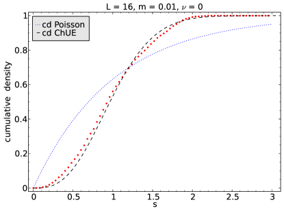
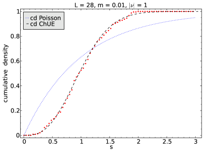
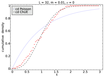
Figure 5: The unfolded level spacing density for the microscopic Dirac spectrum at $m=0.01$ at lattice size $L=16,\ 28$ and $32$. We include the lowest two eigenvalues of configurations with $\nu=0$ ($L=16$ and $32$) and $|\nu|=1$ ($L=28$). The cumulative densities are in all cases close to the Chiral Unitary Ensemble; we do not observe a trend towards the Poisson distribution.

4 Mass anomalous dimension

The numerical measurement of the mass anomalous dimension is a major issue in the recent lattice literature on possibly IR conformal theories.

For its evaluation in the $N_{f}=2$ Schwinger model, we follow here a procedure which was recently applied in Ref. [10]. Thus we consider the mode number

$$\nu_{\rm mode}(\lambda)=V\int_{-\lambda}^{\lambda}d\lambda^{\prime}\ \rho(\lambda^{\prime})\ ,$$ (4.1)

where $\rho$ is the total Dirac spectral density of $D_{\rm ovHF}(m=0)$. This quantity — the cumulative density up to the normalization — contains the same information as $\rho(\lambda)$. It has been studied for $N_{f}=2$ QCD in Ref. [17], where also its renormalizability has been demonstrated.

If $\rho(\lambda)$ is of the form (1.9), we obtain (after mapping the spectrum on ${\kern 2.5pt\sf{R}\kern-7.79999pt\sf{I}\kern 7.79999pt\kern-2.5pt}_{+}$, cf. eq. (2.2))

$$\nu_{\rm mode}(\lambda)=\frac{2cV^{2}}{\alpha+1}\lambda^{\alpha+1}\ .$$ (4.2)

By measuring $\nu_{\rm mode}(\lambda)$ we can identify the exponent, which may be energy dependent, $\alpha(\lambda)$. It is related to the mass anomalous dimension $\gamma_{m}(\lambda)$ as [22]

$$\gamma_{m}(\lambda)=\frac{d}{\alpha(\lambda)+1}-1\ ,$$ (4.3)

where $d$ is the space-time dimension. Free fermions have spectra $\rho(\lambda)\propto\lambda^{d-1}$ [15], hence $\gamma_{m}$ is a measure for the deviation from this behavior due to interactions. In investigations of candidates for IR conformal theories one is most interested in the extrapolation to the IR limit, which is also our focus,

$$\gamma_{m}^{*}=\ ^{\lim}_{\lambda\to 0}\ \gamma_{m}(\lambda)\ .$$ (4.4)

Figure 6 shows our results for $m=0.01$ and $0.06$ and $L=16\dots 32$.

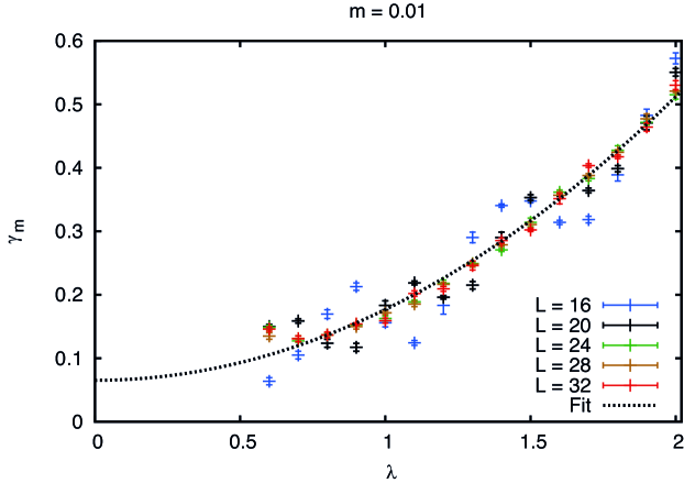
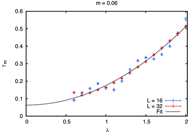
Figure 6: The mass anomalous dimension, determined from the mode number $\nu_{\rm mode}(\lambda)$ in the range $\lambda=0.6\dots 2$. The results at fermion mass $m=0.01$ (above) and $m=0.06$ (below) are very similar; both suggest practically the same IR extrapolation to $\gamma_{m}^{*}$, given in eq. (4.5).

For both masses, the data from various volumes agree quite well in the range $0.6\leq\lambda\leq 2$. This reveals that finite size effects do not affect $\gamma_{m}(\lambda\geq 0.6)$ significantly. Moreover, the data enable a stable IR extrapolation, which agrees very well for both masses. We infer that, in this framework, the chiral extrapolation is not a serious issue either. The two (quadratic) fits in Figure 6 lead to practically the same IR limit,

$$m=0.01 ~{}:~{} \gamma_{m}^{*}=0.065(5)\ ,$$

$$m=0.06 ~{}:~{} \gamma_{m}^{*}=0.063(7)\ .$$ (4.5)

On the other hand, a large Hetrick-Hosotani-Iso parameter, $l\gg 1$, corresponds to $\alpha=1/3$, as we anticipated in Section 1. In this limit we obtain $\gamma_{m}^{*}=0.5$. The opposite limit, $l\ll 1$, leads to $\gamma_{m}^{*}=0$. The value that we determined from the finite size scaling of the cumulative densities $R_{1}$, $R_{2}$, $R_{3}$ in Ref. [26], $\alpha=3/5$, corresponds to $\gamma_{m}^{*}=0.25$. Our fits in Figure 6 are based on a regime of higher energy, so they involve Dirac eigenvalues closer to the bulk. The corresponding IR extrapolation in eq. (4.5) is significantly smaller, and therefore closer to the non-anomalous value $\gamma_{m}^{*}=0$ of free fermions.

5 Conclusions

We have investigated aspects of the 2-flavor Schwinger model, as a simple model with $\Sigma=0$. We first tested Kovács’ conjecture of the decorrelation of low lying Dirac eigenvalues [4]. The cumulative densities of these eigenvalues can be fitted very well to the functions which correspond to this conjecture. Also the mean eigenvalues in various volumes can be fitted well to the predicted form. However, the two fitting parameters take inconsistent values; in particular the exponent $\alpha$ of eq. (1.9) varies over an order of magnitude for different fits.

As for the unfolded level spacing density, this conjecture predicts a Poissonian behavior for a restriction to small Dirac eigenvalues, which turns into the shape of the Chiral Unitary Ensemble if the full spectrum is included. However, we did not observe that property either; as far as we could explore the statistics of the lowest eigenvalues, their unfolded level spacings are close to the distribution of the Chiral Unitary Ensemble, but very far from a Poisson distribution.

Therefore, ultimately the conjecture of low eigenvalue decorrelation cannot be confirmed in this model. On the other hand, this conjecture has been affirmed in the models studied by Kovács and Pittler [4, 30], which dealt with 4d Yang-Mills gauge theories at high temperature. This observation is fully consistent with the refined conjecture that the microscopic eigenvalue decorrelation occurs if $\Sigma$ vanishes due to high temperature. Indeed, according to Ref. [31] the inverse temperature acts as a localization scale for the low lying Dirac eigenmodes. That scenario includes in particular QCD above the temperature of the chiral symmetry restoration.

However, this established property left the question open whether or not the eigenvalue decorrelation also sets in if the chiral condensate vanishes for a different reason. Here we investigated a case where this happens due to a sufficiently large number of fermion flavors, as it is also expected in multi-flavor QCD. Contrary to our initial expectation, the eigenvalue decorrelation conjecture does not lead to a consistent picture in this case. Thus our observation restricts the range of applicability of this interesting conjecture.

Regarding the mass anomalous dimension, this simple model illustrates in a striking manner that the determination of $\gamma_{m}^{*}$ is a very subtle issue. One obtains (apparently) stable results for $\gamma_{m}^{*}$, which, however, strongly depend on the way how the chiral limit and the large volume limit are approached. In general also the continuum limit $g\to 0$ is part of the ordering ambiguity, such that the result for $\gamma_{m}^{*}$ depends on the product $m\sqrt{L^{3}g}$. The formula of Ref. [13], eq. (1.6), refers to the procedure of taking the continuum and infinite volume limits first, and then address the chiral condensate at small fermion mass. However, even if we deal with finite and fixed $g$, $L$ and $m$, the outcome for $\gamma_{m}^{*}$ still depends on the energy interval that we employ for the IR extrapolation, so this quantity is tricky indeed.

This might also provide a hint on why the recent literature on the corresponding quantity for models with many light quarks in $d=4$, interacting through $SU(3)$ gauge fields, is so controversial (cf. Section 1), and why it is particularly hard to determine $\gamma_{m}^{*}$, see e.g. Refs. [7, 10]. The ongoing discussion (and confusion) also includes extensions of QCD regarding the number of colors, and quarks in the adjoint or sextet representation, see Ref. [11] and references therein.

Acknowledgements: Stanislav Shcheredin and Jan Volkholz have contributed to this work at an early stage. We also thank Poul Damgaard, Stephan Dürr, Philippe de Forcrand, James Hetrick, Christian Hoelbling, Tamas Kovács and Andrei Smilga for helpful communication.

This work was supported by the Mexican Consejo Nacional de Ciencia y Tecnología (CONACyT) through project 155905/10 “Física de Partículas por medio de Simulaciones Numéricas”, and by the Croatian Ministry of Science, Education and Sports, project No. 0160013.

References

- [1] D. Mermin and H. Wagner, Phys. Rev. Lett. 17 (1966) 113. P.C. Hohenberg, Phys. Rev. 158 (1967) 383. S.R. Coleman, Commun. Math. Phys. 31 (1973) 259.
- [2] J. Schwinger, Phys. Rev. 128 (1962) 2425. S.R. Coleman, R. Jackiw and L. Susskind, Annals Phys. 93 (1975) 267. S.R. Coleman, Annals Phys. 101 (1976) 239.
- [3] S. Dürr and C. Hoelbling, Phys. Rev. D 69 (2004) 034503.
- [4] T.G. Kovács, Phys. Rev. Lett. 104 (2010) 031601.
- [5] A. Deuzeman, M.P. Lombardo and E. Pallante, Phys. Lett. B 670 (2008) 41. Z. Fodor, K. Holland, J. Kuti, D. Nogradi and C. Schroeder, Phys. Lett. B 681 (2009) 353. P. de Forcrand, S. Kim and W. Unger, JHEP 1302 (2013) 051. K.-I. Ishikawa, Y. Iwasaki, Y. Nakayama and T. Yoshie, Phys. Rev. D 87 (2013) 071503. Y. Aoki et al., Phys. Rev. D 87 (2013) 094511.
- [6] T. Appelquist, G.T. Fleming, M.F. Lin, E.T. Neil and D. Schaich, Phys. Rev. D 84 (2011) 054501. T. DeGrand, Phys. Rev. D 84 (2011) 116901. C.-J.D. Lin, K. Ogawa, H. Ohki and E. Shintani, JHEP 1208 (2012) 096. E. Itou, arXiv:1212.1353.
- [7] A. Cheng, A. Hasenfratz and D. Schaich, Phys. Rev. D 85 (2012) 094509. Y. Aoki et al., Phys. Rev. D 86 (2012) 054506.
- [8] Z. Fodor, K. Holland, J. Kuti, D. Nogradi and C. Schroeder, Phys. Lett. B 703 (2011) 348. X.-Y. Jin and R.D. Mawhinney, PoS(Lattice 2011)066.
- [9] F. Farchioni, I. Hip, C.B. Lang and M. Wohlgenannt, Nucl. Phys. B 549 (1999) 364.
- [10] A. Cheng, A. Hasenfratz, G. Petropoulos and D. Schaich, JHEP 1307 (2013) 061.
- [11] L. Del Debbio, PoS(LATTICE2010)004.
- [12] H.J. Rothe, “Lattice Gauge Theories: An Introduction”, World Scientific (1992). I. Montvay and G. Münster, “Quantum Fields on a Lattice”, Cambridge University Press (1994). C. Gattringer and C.B. Lang, “Quantum Chromodynamics on the Lattice”, Lecture Notes in Physics, Springer (2010).
- [13] A.V. Smilga, Phys. Lett. B 278 (1992) 371; Phys. Rev. D 55 (1997) 443.
- [14] J.E. Hetrick, Y. Hosotani and S. Iso, Phys. Lett. B 350 (1995) 92.
- [15] H. Leutwyler and A.V. Smilga, Phys. Rev. D 46 (1992) 5607.
- [16] T. Banks and A. Casher, Nucl. Phys. B 169 (1980) 103.
- [17] L. Giusti and M. Lüscher, JHEP 0903 (2009) 013.
- [18] P.H. Damgaard and S.M. Nishigaki, Nucl. Phys. B 518 (1998) 495; Phys. Rev. D 63 (2001) 045012.
- [19] F. Farchioni, P. de Forcrand, I. Hip, C.B. Lang and K. Splittorff, Phys. Rev. D 62 (2000) 014503. P.H. Damgaard, U.M. Heller, R. Niclasen and K. Rummukainen, Phys. Rev. D 61 (2000) 014501. B.A. Berg, H. Markum, R. Pullirsch and T. Wettig, Phys. Rev. D 63 (2001) 014504.
- [20] W. Bietenholz, K. Jansen and S. Shcheredin, JHEP 07 (2003) 033. L. Giusti, M. Lüscher, P. Weisz and H. Wittig, JHEP 11 (2003) 023. D. Galletly et al., Nucl. Phys. (Proc. Suppl.) B 129 (2004) 456.
- [21] W. Bietenholz and S. Shcheredin, Nucl. Phys. B 754 (2006) 17.
- [22] L. Del Debbio and R. Zwicky, Phys. Rev. D 82 (2010) 014502.
- [23] W. Bietenholz, Eur. Phys. J. C 6 (1999) 537; Nucl. Phys. B 644 (2002) 223. W. Bietenholz and I. Hip, Nucl. Phys. B 570 (2000) 423.
- [24] H. Neuberger, Phys. Lett. B 417 (1998) 141.
- [25] M. Lüscher, Phys. Lett. B 428 (1998) 342.
- [26] W. Bietenholz, I. Hip, S. Shcheredin and J. Volkholz, Eur. Phys. J. C 72 (2012) 1938.
- [27] P. Hasenfratz, V. Laliena and F. Niedermayer, Phys. Lett. B 427 (1998) 125.
- [28] W.H. Press, S. Teukolsky, W.T. Vetterling und B.P. Flannery, “Numerical Recipes in C++”, Cambridge University Press, 2002.
- [29] M.A. Halasz and J.J.M. Verbaarschot, Phys. Rev. Lett. 74 (1995) 3920.
- [30] T.G. Kovács and F. Pittler, Phys. Rev. D 86 (2012) 114515.
- [31] F. Bruckmann, T.G. Kovács and S. Schierenberg, Phys. Rev. D 84 (2011) 034505.