Spin filtering in a Rashba-Dresselhaus-Aharonov-Bohm double-dot interferometer

Abstract

We study the spin-dependent transport of spin-1/2 electrons through an interferometer made of two elongated quantum dots or quantum nanowires, which are subject to both an Aharonov-Bohm flux and (Rashba and Dresselhaus) spin-orbit interactions. Similar to the diamond interferometer proposed in our previous papers [Phys. Rev. B 84, 035323 (2011); Phys. Rev. B 87, 205438 (2013)], we show that the double-dot interferometer can serve as a perfect spin filter due to a spin interference effect. By appropriately tuning the external electric and magnetic fields which determine the Aharonov-Casher and Aharonov-Bohm phases, and with some relations between the various hopping amplitudes and site energies, the interferometer blocks electrons with a specific spin polarization, independent of their energy. The blocked polarization and the polarization of the outgoing electrons is controlled solely by the external electric and magnetic fields and do not depend on the energy of the electrons. Furthermore, the spin filtering conditions become simpler in the linear-response regime, in which the electrons have a fixed energy. Unlike the diamond interferometer, spin filtering in the double-dot interferometer does not require high symmetry between the hopping amplitudes and site energies of the two branches of the interferometer and thus may be more appealing from an experimental point of view.

1 Introduction

Spin-dependent electrons transport in low-dimensional mesoscopic systems has recently drawn much attention due to its potential for future electronic device applications in the field of spintronics [1, 2, 3, 4]. This new emerging field deals with the active manipulation of the electron’s spin (and not only its charge). Adding the spin degree of freedom to the conventional charge-based technology has the potential advantages of multifunctionality, longer decoherence times and lengths, increased data processing speed, decreased electric power consumption, and increased integration densities compared with conventional semiconductor devices [1, 2]. In addition to the improvement of contemporary technology, spintronics may also contribute to the field of quantum computation and quantum information, in which the quantum information may be contained in the unit vector along which the spin is polarized [5]. Writing and reading information on a spin qubit are thus equivalent to polarizing the spin along a specific direction and identifying the direction along which the spin is polarized, respectively. Hence, a major aim of spintronics is to build mesoscopic spin valves (or spin filters), which generate a tunable spin-polarized current out of unpolarized electron sources. Spin filters can also be used as spin analyzers, which read this information by identifying the polarization directions of incoming polarized beams. A priori, a straightforward way to realize such devices is by using ferromagnets that inject and/or collect polarized electrons [6]. However, connecting ferromagnets to semiconductors is inefficient, due to a large impedance mismatch between them [3, 7, 8, 9, 10]. Therefore, efforts are being made to model and fabricate spintronic devices using intrinsic properties of mesoscopic systems such as strong spin-orbit interaction (SOI). This paradigm of spintronics involves small fields without the need for ferromagnetism at all [11, 12].

In a two-dimensional electron gas (2DEG), formed in mesoscopic structures made of narrow-gap semiconductor heterostructures, the SOI has the general form $\mathcal{H}_{\rm{SO}}=(\hbar k_{\rm{SO}}/m)(\boldsymbol{\pi}\cdot\boldsymbol{\sigma})$ [13]. Here $k_{\rm{SO}}$ characterizes the SOI strength, $\boldsymbol{\pi}$ is a linear combination of the electron momentum components $p_{x}$ and $p_{y}$ and $m$ is the effective mass. The vector of Pauli matrices $\boldsymbol{\sigma}$ is related to the electron spin via $\bi{S}=\hbar\boldsymbol{\sigma}/2$. We distinguish between two special cases of the linear (in the momentum) SOI, namely the Rashba SOI [14, 15] and the Dresselhaus SOI [16]. The Rashba SOI is present in narrow-gap semiconductor heterostructures with a confining potential well which is asymmetric under space inversion. For an electric field perpendicular to the interferometer plane (defined as the $z$ axis), this SOI has the form

$$\mathcal{H}_{\rm{R}}=\frac{\hbar k_{\rm{R}}}{m}\left(p_{y}\sigma_{x}-p_{x}\sigma_{y}\right).$$ (1)

The coefficient $k_{\rm{R}}$ depends on the magnitude of the electric field and can be controlled by a gate voltage, as shown in several experiments [17, 18, 19, 20, 21, 22, 23]. The Dresselhaus SOI is a consequence of a host crystal which lacks bulk inversion symmetry. For a 2DEG the linear Dresselhaus SOI is given by

$$\mathcal{H}_{\rm{D}}=\frac{\hbar k_{\rm{D}}}{m}\left(p_{x}\sigma_{x}-p_{y}\sigma_{y}\right),$$ (2)

where $k_{\rm{D}}$ is a material constant which is proportional to $1/d^{2}$, with $d$ the quantum well thickness [24]. It depends weakly (if at all) on the external field. These SOIs can be interpreted as a Zeeman interaction in a momentum-dependent effective magnetic field. As the electron propagates in the presence of these SOIs, its spin precesses around this effective magnetic field. As a consequence, after propagating a distance $L$ in the direction of the unit vector $\hat{\bi{g}}$, the electron’s spinor $|\chi\rangle$ transforms into $|\chi^{\prime}\rangle=U|\chi\rangle$ with the SU(2) matrix $U=e^{i\bi{K}\cdot\boldsymbol{\sigma}}$ [25, 26]. Here, the vector $\bi{K}$ is

$$\bi{K}=\alpha_{\rm{R}}\left(-g_{y},g_{x},0\right)+\alpha_{\rm{D}}\left(-g_{x},g_{y},0\right),$$ (3)

with the dimensionless coefficients $\alpha_{\rm{R},\rm{D}}\equiv k_{\rm{R},\rm{D}}L$. The SOI-related phase of the unitary matrix $U$ is known as the Aharonov-Casher (AC) phase [27]. Below we use the unitary matrix $U$ and the parameters $\alpha_{\rm{R},\rm{D}}$ to characterize the hopping between adjacent bonds in the presence of SOI.

Recently, several groups proposed spin filters based on a single loop, subject to both electric and magnetic fields perpendicular to the plane of the loop [28, 29, 30]. The phases of these waves include the AC phase and the Aharonov-Bohm (AB) phase [31], which results from a magnetic flux $\Phi$ penetrating the loop. When an electron goes around such a loop, its wave function gains an AB phase $\phi=2\pi\Phi/\Phi_{0}$, where $\Phi_{0}=hc/e$ is the flux quantum ($c$ is the speed of light and $e$ is the electron charge). The combined effect of the SOI and the AB flux is to transform the spinor $|\chi\rangle$ of an electron that goes around a loop into $|\chi^{\prime}\rangle=u|\chi\rangle$, where the unitary matrix $u$ is of the form

$$u=u_{\rm{AB}}u_{\rm{SOI}}=e^{-i\phi+i\boldsymbol{\omega}\cdot\boldsymbol{\sigma}}=e^{-i\phi}\left(\cos\omega+i\sin\omega\>\hat{\boldsymbol{\omega}}\cdot\boldsymbol{\sigma}\right).$$ (4)

Here $u_{\rm{AB}}=e^{-i\phi}\bi{I}$ ($\bi{I}$ is the $2\times 2$ unit matrix) is the diagonal transformation matrix due to the AB flux and $u_{\rm{SOI}}=e^{i\boldsymbol{\omega}\cdot\boldsymbol{\sigma}}$ is the transformation matrix due to the SOI. The latter is a product of matrices of the form $e^{i\bi{K}\cdot\boldsymbol{\sigma}}$ discussed above, each coming from the local SOI on a segment of the loop [30]. We neglect the Zeeman term $\mathcal{H}_{\rm{Z}}=\left(g\mu_{\rm{B}}/2\right)\boldsymbol{\sigma}\cdot\bi{B}$ ($g$ is the Landé factor and $\mu_{\rm{B}}$ is the Bohr magneton). Even though $g$ can be large in low-dimensional systems, the Zeeman term is much smaller than the SOI terms (1) and (2) in the magnetic fields considered.

In a previous paper we proposed a diamond interferometer which combines the AB and AC phases to filter a specific spin direction [30]. The filtered direction can be tuned by the external electric and magnetic fields. Moreover, the transmission of the outgoing spin-polarized electrons can be tuned to unity in a wide range of energies. Recently, we generalized this interferometer by including a possible leakage of electrons out of the interferometer [32]. We have shown that spin filtering is still possible in a non-unitary transport, even though the transmission is inherently less than unity.

A major advantage of the diamond interferometer is that full spin filtering can be achieved independent of the electron energy. However, the conditions for full spin filtering, independent of the electron energy, require perfect symmetry between the two branches of the interferometer [30, 32]. Having fulfilled these symmetry relations, the polarization of the outgoing electrons is independent of energy and completely determined by the AB and AC phases [30, 32] (and therefore by the external electric and magnetic fields perpendicular to the interferometer plane). Unfortunately, realizing a highly symmetric interferometer in experiments may be a difficult task. It is thus desirable to have a perfect spin filtering, independent of the electron energy, in an asymmetric interferometer. As we argue in this paper, this can be achieved by enlarging the number of interferometer parameters (such as hopping and site energies). Below we examine a double-dot interferometer which allows a wide freedom for the various parameters, thereby simplifies the experimental realization. The relations between the various parameters are further simplified if one assumes linear-response regime (namely, low temperatures and bias voltages), in which electron transport occurs at a single energy.

The double-dot interferometer is sketched schematically in figure 1. It consists of two elongated quantum dots (QDs) or quantum nanowires (QNs) which are subject to SOI, and the area of the interferometer is penetrated by an AB flux. Recently, the electrical control of SOI was demonstrated in such InAs self-assembled elongated QDs and nanowires [23, 33, 34, 35, 36]. The wires which connect the QDs/QNs are free of SOI. Using scattering theory in the framework of the tight-binding formalism, we calculate the spin-dependent transmission through this interferometer. We employ a one-dimensional tight-binding model, assuming that the interferometer is composed of quasi one-dimensional wires [30, 32].

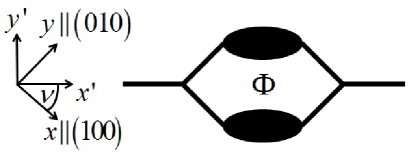
Figure 1: The double-dot interferometer. The interferometer is penetrated by a magnetic flux $\Phi$, and its horizontal edges (of length $L$, shown by the dark ellipses in the figure) are subject to spin-orbit interactions. The $x$ and $y$ axes are parallel to the crystallographic $(100)$ and $(010)$ axes.

The paper is organized as follows: in Sec. 2 we first define the tight-binding model which we use to study electron transport in the double-dot interferometer and solve for the transmission of an arbitrary interferometer (Sec. 2.1). Then we find the general conditions for full filtering (Sec. 2.2). Finally, we find specific criteria for spin filtering in the presence of Rashba and Dresselhaus SOIs (Sec. 2.3). The results are discussed and summarized in Sec. 3.

2 Double-dot interferometer

2.1 Tight-binding model for the double-dot interferometer

To study the scattering of a spin-1/2 electron by the double-dot interferometer with arbitrary SOI and AB flux (figure 1), we model it as a square interferometer as shown in figure 2. Each QD/QN is replaced by a bond connecting two sites ($a$, $b$ and $c$, $d$ in figure 2) with the corresponding bonds subject to SOI. We emphasize that the solution is not limited to this model. One can model each QD/QN by an arbitrary number of sites $M$. This changes only the transmission of the spin-polarized electrons, with no significant effect on the spin filtering conditions and the polarization direction of the outgoing electrons [32].

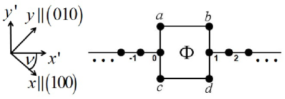
Figure 2: Tight-binding model of the double-dot interferometer. The bonds $ab$ and $cd$ (of length $L$) are subject to spin-orbit interactions.

In the framework of the nearest neighbors tight-binding model, the Schrödinger equation for the spinor $|\psi_{v}\rangle$ at site $v$ is written as

$$\left(\varepsilon-\varepsilon_{v}\right)|\psi_{v}\rangle=-\sum_{u}J_{uv}U_{uv}|\psi_{u}\rangle,$$ (5)

where $\varepsilon_{v}$ is the site energy, $J_{uv}$ is a real hopping amplitude and $U_{uv}$ is a $2\times 2$ unitary matrix which describes the AB and AC phases acquired by an electron moving from site $u$ to site $v$. The sum in equation (5) is over the nearest neighbors $u$ of $v$. At this stage we do not specify the details of these matrices and hopping amplitudes. Except for the sites $0$, $a$, $b$, $c$, $d$ and $1$ (figure 2), the hopping amplitude along the leads is $j$ and the site energies on the leads are set to zero. The leads are free of SOI. Thus, the dispersion relation of the leads is $\varepsilon=-2j\cos\left(ka\right)$ with $a$ the lattice constant. The tight-binding Schrödinger equations for the spinors at sites $0$, $a$, $b$, $c$, $d$ and $1$ are

$$\left(\varepsilon-\varepsilon_{0}\right)|\psi_{0}\rangle=-J_{0a}U^{{\dagger}}_{0a}|\psi_{a}\rangle-J_{0c}U^{{\dagger}}_{0c}|\psi_{c}\rangle-j|\psi_{-1}\rangle,$$

$$\left(\varepsilon-\varepsilon_{a}\right)|\psi_{a}\rangle=-J_{ab}U^{{\dagger}}_{ab}|\psi_{b}\rangle-J_{0a}U_{0a}|\psi_{0}\rangle,$$

$$\left(\varepsilon-\varepsilon_{b}\right)|\psi_{b}\rangle=-J_{b1}U^{{\dagger}}_{b1}|\psi_{1}\rangle-J_{ab}U_{ab}|\psi_{a}\rangle,$$

$$\left(\varepsilon-\varepsilon_{c}\right)|\psi_{c}\rangle=-J_{cd}U^{{\dagger}}_{cd}|\psi_{d}\rangle-J_{0c}U_{0c}|\psi_{0}\rangle,$$

$$\left(\varepsilon-\varepsilon_{d}\right)|\psi_{d}\rangle=-J_{d1}U^{{\dagger}}_{d1}|\psi_{1}\rangle-J_{cd}U_{cd}|\psi_{c}\rangle,$$

$$\left(\varepsilon-\varepsilon_{1}\right)|\psi_{1}\rangle=-j|\psi_{2}\rangle-J_{b1}U_{b1}|\psi_{b}\rangle-J_{d1}U_{d1}|\psi_{d}\rangle.$$ (6)

Eliminating $|\psi_{a}\rangle$, $|\psi_{b}\rangle$, $|\psi_{c}\rangle$ and $|\psi_{d}\rangle$ from equations (2.1) one ends up with the equations

$$\left(\varepsilon-y_{0}\right)|\psi_{0}\rangle=\bi{W}^{{\dagger}}|\psi_{1}\rangle-j|\psi_{-1}\rangle,$$

$$\left(\varepsilon-y_{1}\right)|\psi_{1}\rangle=-j|\psi_{2}\rangle+\bi{W}|\psi_{0}\rangle,$$ (7)

where

$$y_{0}=\varepsilon_{0}+\frac{J^{2}_{0a}}{\varepsilon-\varepsilon_{a}-\frac{J^{2}_{ab}}{\varepsilon-\varepsilon_{b}}}+\frac{J^{2}_{0c}}{\varepsilon-\varepsilon_{c}-\frac{J^{2}_{cd}}{\varepsilon-\varepsilon_{d}}},$$

$$y_{1}=\varepsilon_{1}+\frac{J^{2}_{b1}}{\varepsilon-\varepsilon_{b}-\frac{J^{2}_{ab}}{\varepsilon-\varepsilon_{a}}}+\frac{J^{2}_{d1}}{\varepsilon-\varepsilon_{d}-\frac{J^{2}_{cd}}{\varepsilon-\varepsilon_{c}}},$$ (8)

and

$$\bi{W} =\frac{J_{0a}J_{ab}J_{b1}}{J^{2}_{ab}-\left(\varepsilon-\varepsilon_{a}\right)\left(\varepsilon-\varepsilon_{b}\right)}U_{b1}U_{ab}U_{0a}+\frac{J_{0c}J_{cd}J_{d1}}{J^{2}_{cd}-\left(\varepsilon-\varepsilon_{c}\right)\left(\varepsilon-\varepsilon_{d}\right)}U_{d1}U_{cd}U_{0c}$$ (9)

$$\equiv\gamma_{\rm{upper}}U_{\rm{upper}}+\gamma_{\rm{lower}}U_{\rm{lower}}.$$

Here, the coefficients $\gamma_{\rm{upper}}$ and $\gamma_{\rm{lower}}$ are defined as

$$\gamma_{\rm{upper}}=\frac{J_{0a}J_{ab}J_{b1}}{J^{2}_{ab}-\left(\varepsilon-\varepsilon_{a}\right)\left(\varepsilon-\varepsilon_{b}\right)},$$

$$\gamma_{\rm{lower}}=\frac{J_{0c}J_{cd}J_{d1}}{J^{2}_{cd}-\left(\varepsilon-\varepsilon_{c}\right)\left(\varepsilon-\varepsilon_{d}\right)},$$ (10)

and $U_{\rm{lower}}=U_{d1}U_{cd}U_{0c}$, $U_{\rm{upper}}=U_{b1}U_{ab}U_{0a}$ are the unitary matrices corresponding to transitions through the lower and upper paths of the interferometer, respectively. Equations (2.1) describe the effective tight-binding equations for hopping between sites $0$ and $1$ and have the same form as in the diamond interferometer [30, 32]. All the details of the interferometer are embodied in the effective hopping matrix $\bi{W}$ and effective site energies $y_{0}$ and $y_{1}$.

We next consider the scattering of a wave coming from the left, i.e.

$$|\psi_{n}\rangle=|\chi_{\rm{in}}\rangle e^{ikna}+r|\chi_{\rm{r}}\rangle e^{-ikna},\qquad n\leq 0,$$

$$|\psi_{n}\rangle=t|\chi_{\rm{t}}\rangle e^{ik\left(n-1\right)a},\qquad n\geq 1,$$ (11)

where $|\chi_{\rm{in}}\rangle$, $|\chi_{\rm{r}}\rangle$ and $|\chi_{\rm{t}}\rangle$ are the incoming, reflected and transmitted normalized spinors, respectively, with the corresponding reflection and transmission amplitudes $r$ and $t$. Substituting equations (2.1) into (2.1), one finds

$$t|\chi_{\rm{t}}\rangle\equiv\mathcal{T}|\chi_{\rm{in}}\rangle,\qquad r|\chi_{\rm{r}}\rangle\equiv\mathcal{R}|\chi_{\rm{in}}\rangle,$$ (12)

with the $2\times 2$ transmission and reflection amplitude matrices

$$\mathcal{T}=2ij\sin\left(ka\right)\bi{W}\left(Y\bi{I}-\bi{W}^{{\dagger}}\bi{W}\right)^{-1},$$ (13)

$$\mathcal{R}=-\bi{I}-2ij\sin\left(ka\right)X_{1}\left(Y\bi{I}-\bi{W}^{{\dagger}}\bi{W}\right)^{-1}.$$ (14)

Here we define

$$X_{0,1}=y_{0,1}+je^{-ika},\quad Y=X_{0}X_{1}.$$ (15)

Using equation (9), the matrix $\bi{W}^{{\dagger}}\bi{W}$ involved in both $\mathcal{T}$ and $\mathcal{R}$, is found to be

$$\bi{W}^{{\dagger}}\bi{W}=\gamma^{2}_{\rm{upper}}+\gamma^{2}_{\rm{lower}}+\gamma_{\rm{upper}}\gamma_{\rm{lower}}\left(u+u^{{\dagger}}\right),$$ (16)

with $u=U^{{\dagger}}_{\rm{upper}}U_{\rm{lower}}$ the unitary matrix representing anticlockwise hopping from site $0$ back to site $0$ around the loop. Equation (4) then yields $u+u^{{\dagger}}=2\left(\cos\omega\cos\phi+\sin\omega\sin\phi\>\hat{\boldsymbol{\omega}}\cdot\boldsymbol{\sigma}\right)$ and equation (16) can thus be written as

$$\bi{W}^{{\dagger}}\bi{W}=A+\bi{B}\cdot\boldsymbol{\sigma},$$ (17)

with

$$A=\gamma^{2}_{\rm{upper}}+\gamma^{2}_{\rm{lower}}+2\gamma_{\rm{upper}}\gamma_{\rm{lower}}\cos\omega\cos\phi,$$

$$\bi{B}=2\gamma_{\rm{upper}}\gamma_{\rm{lower}}\sin\omega\sin\phi\>\hat{\bi{n}}\equiv B\hat{\bi{n}}.$$ (18)

Here, $\hat{\bi{n}}\equiv\hat{\boldsymbol{\omega}}$ is a real unit vector along the direction of $\boldsymbol{\omega}$. As shown in [30], the spin-dependent transmission of the interferometer is determined by the eigenvalues of the matrix $\bi{W}^{{\dagger}}\bi{W}$. These eigenvalues are given by

$$\bi{W}^{{\dagger}}\bi{W}|\pm\hat{\bi{n}}\rangle=\lambda_{\pm}|\pm\hat{\bi{n}}\rangle,$$

$$\lambda_{\pm}=A\pm B=\gamma^{2}_{\rm{lower}}+\gamma^{2}_{\rm{upper}}+2\gamma_{\rm{lower}}\gamma_{\rm{upper}}\cos\left(\phi\mp\omega\right),$$ (19)

where $|\pm\hat{\bi{n}}\rangle$ are the eigenstates of the spin component along the unit vector $\hat{\bi{n}}$, i.e. $\hat{\bi{n}}\cdot\boldsymbol{\sigma}|\pm\hat{\bi{n}}\rangle=\pm|\pm\hat{\bi{n}}\rangle$. For an incoming spinor $|\pm\hat{\bi{n}}\rangle$ the corresponding transmission amplitudes $t_{\pm}$ are [30]

$$|t_{\pm}|=\frac{2j\sin\left(ka\right)}{|Y-\lambda_{\pm}|}\sqrt{\lambda_{\pm}},$$ (20)

and the outgoing electrons are polarized along a different direction $\pm\hat{\bi{n}}^{\prime}$, i.e. their spinor is $|\chi^{\rm{out}}_{\pm}\rangle=|\pm\hat{\bi{n}}^{\prime}\rangle$. Hence, the transmission amplitude matrix (13) can be rewritten as

$$\mathcal{T}=t_{-}|-\hat{\bi{n}}^{\prime}\rangle\langle-\hat{\bi{n}}|+t_{+}|\>\hat{\bi{n}}^{\prime}\rangle\langle\hat{\bi{n}}|.$$ (21)

Here, $|\pm\hat{\bi{n}}^{\prime}\rangle$ are the eigenstates of the matrix $\bi{W}\bi{W}^{{\dagger}}$ [30], namely

$$\bi{W}\bi{W}^{{\dagger}}|\pm\hat{\bi{n}}^{\prime}\rangle=\lambda_{\pm}|\pm\hat{\bi{n}}^{\prime}\rangle,$$ (22)

where the eigenvalues $\lambda_{\pm}$ are given by equations (2.1). Using equation (9), the matrix $\bi{W}\bi{W}^{{\dagger}}$ is given by

$$\bi{W}\bi{W}^{{\dagger}}=\gamma^{2}_{\rm{upper}}+\gamma^{2}_{\rm{lower}}+\gamma_{\rm{upper}}\gamma_{\rm{lower}}\left(u^{\prime}+u^{\prime{\dagger}}\right),$$ (23)

with $u^{\prime}=U_{\rm{upper}}U^{{\dagger}}_{\rm{lower}}$ the unitary matrix representing clockwise hopping from site $1$ back to site $1$ around the loop.

It is important to emphasize that the spinors $|\pm\hat{\bi{n}}\rangle$ and $|\pm\hat{\bi{n}}^{\prime}\rangle$, being the eigenstates of $u+u^{{\dagger}}$ and $u^{\prime}+u^{\prime{\dagger}}$, respectively, are completely determined by the AB and AC phases and are independent of the electron energy $\varepsilon$. As we show below, this implies that spin filtering can be achieved independent of energy, with the spin polarization direction controlled solely by the external electric and magnetic fields (see below). In the next subsection we analyze the general conditions for spin filtering arising from the transmission amplitude matrix (21) with the transmission amplitudes (20).

2.2 General conditions for spin filtering in the double-dot interferometer

The spin-polarized current (along $\hat{\bi{n}}^{\prime}$) at the output of the interferometer is given by [37]

$$I=\frac{e}{\hbar}\int^{\infty}_{-\infty}\frac{d\varepsilon}{2\pi}\left[f_{\rm{L}}(\varepsilon)-f_{\rm{R}}(\varepsilon)\right]P_{\hat{\bi{n}}^{\prime}}(\varepsilon)\Tr\left[\mathcal{T}^{{\dagger}}\mathcal{T}\right],$$ (24)

where $f_{\rm{L},\rm{R}}(\varepsilon)=\left[1+e^{\left(\varepsilon-\mu_{\rm{L},\rm{R}}\right)/k_{\rm{B}}T}\right]^{-1}$ is the Fermi distribution in the left (L) or right (R) lead with the corresponding chemical potential $\mu_{\rm{L}}$ and $\mu_{\rm{R}}$, $k_{\rm{B}}$ is the Boltzmann constant and $T$ is the temperature. The spin polarization $P_{\hat{\bi{n}}^{\prime}}(\varepsilon)$ along $\hat{\bi{n}}^{\prime}$ is defined as

$$P_{\hat{\bi{n}}^{\prime}}(\varepsilon)\equiv\frac{\Tr\left[\mathcal{T}^{{\dagger}}\mathcal{T}\boldsymbol{\sigma}\cdot\hat{\bi{n}}^{\prime}\right]}{\Tr\left[\mathcal{T}^{{\dagger}}\mathcal{T}\right]}=\frac{|t_{+}|^{2}-|t_{-}|^{2}}{|t_{+}|^{2}+|t_{-}|^{2}},$$ (25)

where in the last step we used equation (21). For $P_{\hat{\bi{n}}^{\prime}}(\varepsilon)=\pm 1$ the outgoing electrons with energy $\varepsilon$ are fully polarized along $\pm\hat{\bi{n}}^{\prime}$. This occurs if and only if $|t_{\mp}|=0$, or equivalently $\lambda_{\mp}=0$ [equation (20)]. Without loss of generality, let us consider the case $\lambda_{-}=0$, in which the outgoing electrons are polarized along $\hat{\bi{n}}^{\prime}$. From equation (2.1) it follows that $\lambda_{\pm}\geq 0$ and the equality $\lambda_{-}=0$ occurs only if

$$\gamma_{\rm{lower}}=\gamma_{\rm{upper}}\equiv\gamma,$$

$$\cos(\phi+\omega)=-1.$$ (26)

It should be noted that the spin filtering conditions (2.2) are valid for an arbitrary two-path interferometer with SOI and AB flux. The details of a specific interferometer enter through the AC phase $\omega$ and the effective hopping amplitudes $\gamma_{\rm{lower}}$ and $\gamma_{\rm{upper}}$. The first condition in equations (2.2) can be interpreted as a requirement for a symmetry relation between the two paths. The second condition in equations (2.2), namely $\omega=-\phi+\pi$, imposes a relation between the AB flux and the SOI strength.

To achieve an outgoing spin-polarized beam at finite temperature or bias voltage, the spin polarization $P_{\hat{\bi{n}}^{\prime}}(\varepsilon)$ should be equal to unity in the relevant energies $\mu_{\rm{R}}-(\rm a\ \rm f\rm e\rm w\ k_{\rm{B}}T)<\varepsilon<\mu_{\rm{L}}+(\rm a\ \rm f\rm e\rm w\ k_{\rm{B}}T)$ in which electron transport occurs. Therefore, it is desirable that the spin filtering conditions (2.2) will be satisfied independent of energy. Since the second condition in equations (2.2) is energy independent, we focus for the moment on the first condition. From equations (2.1), one readily sees that this condition holds independent of energy if

$$J_{0a}J_{ab}J_{b1}=J_{0c}J_{cd}J_{d1},$$

$$\varepsilon_{a}+\varepsilon_{b}=\varepsilon_{c}+\varepsilon_{d},$$

$$J^{2}_{ab}-\varepsilon_{a}\varepsilon_{b}=J^{2}_{cd}-\varepsilon_{c}\varepsilon_{d}.$$ (27)

Compared to the corresponding relations in the diamond interferometer [30, 32], equations (2.2) allow much more freedom for the values of the various parameters (see below). Therefore, spin filtering can be achieved even in a very asymmetric interferometer. Furthermore, as argued at the end of the previous subsection, the spinor of the outgoing electrons, $|\hat{\bi{n}}^{\prime}\rangle$, is independent of energy. Hence, the spin filtering is energy independent provided that equations (2.2) hold.

To satisfy equations (2.2), one can adopt several approaches. One possibility is to use a single gate electrode for each branch of the interferometer, so that $\varepsilon_{a}=\varepsilon_{b}\equiv\varepsilon_{ab}$ and $\varepsilon_{c}=\varepsilon_{d}\equiv\varepsilon_{cd}$. The conditions (2.2) then read

$$J_{0a}J_{b1}=J_{0c}J_{d1},$$

$$\varepsilon_{ab}=\varepsilon_{cd},$$

$$J_{ab}=J_{cd}.$$ (28)

The first condition in equations (2.2) can be satisfied by properly tuning the hopping amplitudes from the leads to the QDs/QNs, as shown in several experiments [38, 39, 40, 41]. The second condition can be satisfied by tuning the gate electrodes. The third condition can be satisfied by controlling the potential barrier between sites $a$ and $b$ (and/or $c$ and $d$). A further possibility to satisfy equations (2.2) is by using two gate electrodes on each branch of the interferometer [35]. Then, by tuning two site energies, say $\varepsilon_{a}$ and $\varepsilon_{c}$, one can fulfill the second and the third conditions in equations (2.2). The first condition is again satisfied by tuning one of the hopping amplitudes from the leads to the QDs/QNs, say $J_{b1}$.

Alternatively, one can work at low temperatures in the linear-response regime, where all the electrons have the same energy, equal to the Fermi energy of the leads $\varepsilon_{\rm{F}}$. The first condition in equations (2.2) should then be satisfied for a single specific energy $\varepsilon=\varepsilon_{\rm{F}}$. Setting $\varepsilon_{\rm{F}}=0$ in equations (2.1), one has

$$\frac{J_{0a}J_{ab}J_{b1}}{J^{2}_{ab}-\varepsilon_{a}\varepsilon_{b}}=\frac{J_{0c}J_{cd}J_{d1}}{J^{2}_{cd}-\varepsilon_{c}\varepsilon_{d}}.$$ (29)

In this case one has to tune only a single site energy $\tilde{\varepsilon}=\varepsilon_{a}=\varepsilon_{b}$. In addition, one should tune the magnetic field or the electric field perpendicular to the plane in order to satisfy the second condition in equations (2.2).

Having fulfilled the spin filtering conditions (2.2), one would like to optimize the transmission $T_{+}=|t_{+}|^{2}$ of the polarized electrons. Using equation (20), the transmission has the form [30]

$$T_{+}=|t_{+}|^{2}=\frac{4j^{2}\sin^{2}\left(ka\right)\lambda_{+}}{P+Q\cos\left(ka\right)+R\cos\left(2ka\right)},$$ (30)

where

$$P=\left(y_{0}y_{1}-\lambda_{+}\right)^{2}+\left(y_{0}+y_{1}\right)^{2}j^{2}+j^{4},$$

$$Q=2j\left(y_{0}y_{1}-\lambda_{+}+j^{2}\right)\left(y_{0}+y_{1}\right),$$

$$R=2j^{2}\left(y_{0}y_{1}-\lambda_{+}\right).$$ (31)

The dependence of the transmission on the magnetic flux is only through $\lambda_{+}$. Substituting $\omega=-\phi+\pi$ and $\gamma_{\rm{lower}}=\gamma_{\rm{upper}}=\gamma$ into equations (2.1), one has $\lambda_{+}=4\gamma^{2}\sin^{2}\phi$. Since one does not expect the tight-binding model to be valid near the band edges, we confine ourselves to the center of the band, $\varepsilon=0$ or $ka=\pi/2$, where the details of the model chosen are not so important. At the band center we have $\gamma(\varepsilon=0)\equiv\gamma_{0}=J^{3}_{1}/J^{2}_{2}$ with $J^{3}_{1}\equiv J_{0a}J_{ab}J_{b1}=J_{0c}J_{cd}J_{d1}$ and $J^{2}_{2}\equiv J^{2}_{ab}-\varepsilon_{a}\varepsilon_{b}=J^{2}_{cd}-\varepsilon_{c}\varepsilon_{d}$, as required by equations (2.2). The denominator in equation (13) becomes $P-R=\Big{\{}\left[\varepsilon_{0}+\left(J^{2}_{0a}\varepsilon_{b}+J^{2}_{0c}\varepsilon_{d}\right)\gamma_{0}/J^{3}_{1}\right]\left[\varepsilon_{1}+\left(J^{2}_{b1}\varepsilon_{a}+J^{2}_{d1}\varepsilon_{c}\right)\gamma_{0}/J^{3}_{1}\right]-\lambda_{+}-j^{2}\Big{\}}^{2}+j^{2}\left[\varepsilon_{0}+\varepsilon_{1}+\left(J^{2}_{0a}\varepsilon_{b}+J^{2}_{0c}\varepsilon_{d}+J^{2}_{b1}\varepsilon_{a}+J^{2}_{d1}\varepsilon_{c}\right)\gamma_{0}/J^{3}_{1}\right]^{2}$, which is minimal at $\varepsilon_{0}=-\left(J^{2}_{0a}\varepsilon_{b}+J^{2}_{0c}\varepsilon_{d}\right)\gamma_{0}/J^{3}_{1}$ and $\varepsilon_{1}=-\left(J^{2}_{b1}\varepsilon_{a}+J^{2}_{d1}\varepsilon_{c}\right)\gamma_{0}/J^{3}_{1}$. In this case the transmission is $T_{+}=4j^{2}\lambda_{+}/(\lambda_{+}+j^{2})^{2}$, and this has its maximal value of $1$ at $\lambda_{+}=j^{2}$. For a specific filter one would usually decide around which flux $\phi_{0}$ one would like to work. We thus optimize the transmission for a specific flux $\phi=\phi_{0}$. One has a perfect transmission $T_{+}(\varepsilon=0,\phi=\phi_{0})=1$ at a flux $\phi=\phi_{0}$ if one tunes the parameters so that $\gamma_{0}=J^{3}_{1}/J^{2}_{2}=j/\left(2\sin\phi_{0}\right)$, $\varepsilon_{0}=-\left(J^{2}_{0a}\varepsilon_{b}+J^{2}_{0c}\varepsilon_{d}\right)\gamma_{0}/J^{3}_{1}$ and $\varepsilon_{1}=-\left(J^{2}_{b1}\varepsilon_{a}+J^{2}_{d1}\varepsilon_{c}\right)\gamma_{0}/J^{3}_{1}$. With these choices, the transmission $T_{+}(\varepsilon=0,\phi)$ reads

$$T_{+}(\varepsilon=0,\phi)=\frac{4\sin^{2}\phi\sin^{2}\phi_{0}}{\left(\sin^{2}\phi+\sin^{2}\phi_{0}\right)^{2}}.$$ (32)

The transmission (32) is plotted in figure 3(a) as a function of $\phi$ for two values of $\phi_{0}$. Figure 3(b) shows the transmission $T_{+}$ versus $ka$ for the flux fixed at $\phi=\phi_{0}$ and for $J_{0a}=J_{b1}=J_{0c}=J_{d1}=2j$, $J_{ab}=J_{cd}=8j$ and $\varepsilon_{a}=\varepsilon_{b}=\varepsilon_{c}=\varepsilon_{d}=\sqrt{J^{2}_{ab}-J^{3}_{1}/\gamma_{0}}$. These values correspond to a completely symmetric interferometer in which the hopping amplitudes and site energies of the lower and upper branches are identical. The transmission depends smoothly on energy and remains close to unity in a range around $ka=\pi/2$ which increases with increasing $\phi_{0}$. As expected, the transmission in this case resembles the transmission of the symmetric diamond interferometer [30].

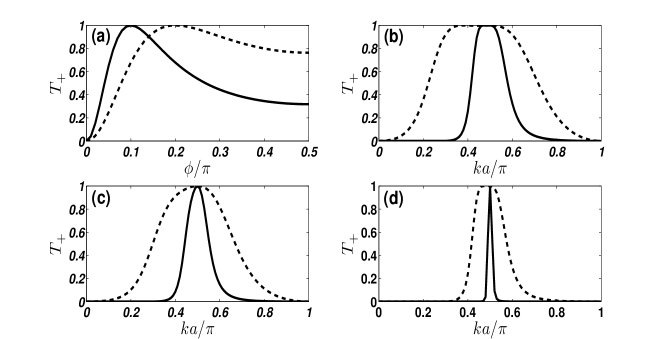
Figure 3: The transmission of the polarized electrons, $T_{+}(\epsilon,\phi)$ (a) as a function of the AB flux $\phi$ (in units of $\pi$) for $\epsilon=0$ ($ka=\pi/2$) and (b), (c), (d) as a function of $ka$ (in units of $\pi$) for $\phi=\phi_{0}$. Solid and dashed curves correspond to maxima of $T_{+}(\epsilon=0,\phi)$ at $\phi_{0}=0.1\pi$ and $\phi_{0}=0.2\pi$, respectively. This is achieved by choosing $\gamma_{0}=J^{3}_{1}/J^{2}_{2}=j/\left(2\sin\phi_{0}\right)$, $\varepsilon_{0}=-\left(J^{2}_{0a}\varepsilon_{b}+J^{2}_{0c}\varepsilon_{d}\right)\gamma_{0}/J^{3}_{1}$ and $\varepsilon_{1}=-\left(J^{2}_{b1}\varepsilon_{a}+J^{2}_{d1}\varepsilon_{c}\right)\gamma_{0}/J^{3}_{1}$. The values of the hopping amplitudes and the other site energies are (b) $J_{0a}=J_{b1}=J_{0c}=J_{d1}=2j$, $J_{ab}=J_{cd}=8j$ and $\varepsilon_{a}=\varepsilon_{b}=\varepsilon_{c}=\varepsilon_{d}=\sqrt{J^{2}_{ab}-J^{3}_{1}/\gamma_{0}}$, (c) $J_{0a}=j$, $J_{b1}=4j$, $J_{0c}=J_{d1}=2j$, $J_{ab}=J_{cd}=8j$ and $\varepsilon_{a}=\varepsilon_{b}=\varepsilon_{c}=\varepsilon_{d}=\sqrt{J^{2}_{ab}-J^{3}_{1}/\gamma_{0}}$, (d) $J_{0a}=J_{b1}=J_{d1}=2j$, $J_{0c}=1.6j$, $J_{ab}=8j$, $J_{cd}=10j$ and $\varepsilon_{a}=j$.

Figures 3(c) and 3(d) are the same as figure 3(b) but for an asymmetric interferometer. In figure 3(c) we set $J_{0a}=j$, $J_{b1}=4j$, $J_{0c}=J_{d1}=2j$, $J_{ab}=J_{cd}=8j$ and $\varepsilon_{a}=\varepsilon_{b}=\varepsilon_{c}=\varepsilon_{d}=\sqrt{J^{2}_{ab}-J^{3}_{1}/\gamma_{0}}$. This choice corresponds to an asymmetric interferometer described by equations (2.2), in which the two branches have the same site energies $\varepsilon_{a}=\varepsilon_{b}=\varepsilon_{c}=\varepsilon_{d}$ and hopping amplitudes $J_{ab}=J_{cd}$, but different hopping amplitudes from the leads, namely $J_{0a}\neq J_{0c}$ and $J_{b1}\neq J_{d1}$. Figure 3(d) shows the transmission of a completely asymmetric interferometer for which $J_{0a}=J_{b1}=J_{d1}=2j$, $J_{0c}=1.6j$, $J_{ab}=8j$, $J_{cd}=10j$ and $\varepsilon_{a}\neq\varepsilon_{b}\neq\varepsilon_{c}\neq\varepsilon_{d}$. We set $\varepsilon_{a}=j$ and then the values of $\varepsilon_{b}$, $\varepsilon_{c}$ and $\varepsilon_{b}$ are determined from equations (2.2) and from the equation $\gamma_{0}=J^{3}_{1}/J^{2}_{2}=j/\left(2\sin\phi_{0}\right)$. A comparison between figures 3(b)-3(d) reveals that the transmission peak at $ka=\pi/2$ gets narrower as the interferometer becomes more asymmetric. However, comparing the solid and dashed curves in figures 3(b)-3(d), we see that the narrowing of the transmission peak can be circumvented by working at a higher flux $\phi=\phi_{0}$.

The results of this subsection thus suggest that perfect spin filtering, independent of energy, can be accomplished in an asymmetric interferometer. By tuning the hopping amplitudes, site energies and AB flux, one can simultaneously satisfy the conditions (2.2) and obtain an ideal transmission of the spin-polarized electrons. The polarization direction of these spin-polarized outgoing electrons is discussed in the next subsection.

2.3 Spin filtering conditions in the presence of Rashba and Dresselhaus SOIs

Let us consider now the form of the unitary matrices $U_{uv}=e^{i\phi_{uv}+i\bi{K}_{uv}\cdot\boldsymbol{\sigma}}$ in the presence of Rashba and Dresselhaus SOIs. First, consider the AB phase $\phi_{uv}=-\frac{e}{\hbar}\int^{v}_{u}\bi{A}\cdot\bi{dr}$. With the gauge $\bi{A}=-By^{\prime}\hat{\bi{x}}^{\prime}$ (figure 2), the AB phases are nonzero only for the bonds $ab$ and $cd$, with the latter being $\phi_{ab}=-\phi_{cd}=\phi/2$. To account for the Rashba and Dresselhaus SOIs, we denote the angle between the $x$ axis and the crystallographic $(100)$ axis as $\nu$ (figure 2). With respect to the crystallographic axes, the unit vectors along the bonds $ab$ and $cd$ are then $\hat{\bi{g}}_{ab}=\hat{\bi{g}}_{cd}=(\cos\nu,\sin\nu,0)$. Using equation (3) and denoting

$$\alpha^{2}_{uv}=\alpha^{2}_{\rm{R},uv}+\alpha^{2}_{\rm{D},uv},\quad\tan\theta_{uv}=\alpha_{\rm{D},uv}/\alpha_{\rm{R},uv}\quad(uv=ab,cd),$$ (33)

one ends up with the unitary matrices

$$U_{ab}=e^{i\phi/2+i\alpha_{ab}\sigma_{ab}},\quad U_{cd}=e^{-i\phi/2+i\alpha_{cd}\sigma_{cd}},$$

$$U_{0a}=U_{b1}=U_{0c}=U_{d1}=\bi{I},$$ (34)

where $\sigma_{uv}=-\sin\xi_{uv}\sigma_{x}+\cos\psi_{uv}\sigma_{y}$, with $\xi_{uv}=\theta_{uv}+\nu$ and $\psi_{uv}=\theta_{uv}-\nu$ ($uv=ab,cd$). Note that $\sigma^{2}_{uv}=F^{2}_{uv}=1+\sin\left(2\nu\right)\sin\left(2\theta_{uv}\right)$ and therefore $e^{i\alpha_{uv}\sigma_{uv}}=c_{uv}+is_{uv}\sigma_{uv}$, with $c_{uv}=\cos\left(\alpha_{uv}F_{uv}\right)$ and $s_{uv}=\sin\left(\alpha_{uv}F_{uv}\right)/F_{uv}$. To identify the AC phase $\omega$ and the blocked and transmitted spin directions, $-\hat{\bi{n}}$ and $\hat{\bi{n}}^{\prime}$, we calculate the matrices $u=U^{{\dagger}}_{\rm{upper}}U_{\rm{lower}}=U^{{\dagger}}_{ab}U_{cd}$ and $u^{\prime}=U_{\rm{upper}}U^{{\dagger}}_{\rm{lower}}=U_{ab}U^{{\dagger}}_{cd}$. Straightforward algebra yields

$$u=e^{-i\phi}e^{-i\alpha_{ab}\sigma_{ab}}e^{i\alpha_{cd}\sigma_{cd}}=e^{-i\phi}\left(\delta+i\boldsymbol{\tau}\cdot\boldsymbol{\sigma}\right),$$

$$u^{\prime}=e^{i\phi}e^{i\alpha_{ab}\sigma_{ab}}e^{-i\alpha_{cd}\sigma_{cd}}=e^{i\phi}\left(\delta+i\boldsymbol{\tau}^{\prime}\cdot\boldsymbol{\sigma}\right),$$ (35)

where

$$\delta=c_{ab}c_{cd}+s_{ab}s_{cd}\left(\sin\xi_{ab}\sin\xi_{cd}+\cos\psi_{ab}\cos\psi_{cd}\right),$$

$$\tau_{x}=-\tau^{\prime}_{x}=s_{ab}c_{cd}\sin\xi_{ab}-s_{cd}c_{ab}\sin\xi_{cd},$$

$$\tau_{y}=-\tau^{\prime}_{y}=s_{cd}c_{ab}\cos\psi_{cd}-s_{ab}c_{cd}\cos\psi_{ab},$$

$$\tau_{z}=\tau^{\prime}_{z}=s_{ab}s_{cd}\left(\sin\xi_{cd}\cos\psi_{ab}-\sin\xi_{ab}\cos\psi_{cd}\right),$$ (36)

and $\delta^{2}+|\boldsymbol{\tau}|^{2}=1$ from unitarity. Comparing equations (2.3) with (16), (2.1), (22) and (23), one derives the following relations:

$$\cos\omega=\delta,\quad\hat{\bi{n}}=\hat{\boldsymbol{\tau}},\quad\hat{\bi{n}}^{\prime}=-\hat{\boldsymbol{\tau}}^{\prime}.$$ (37)

Equations (2.3) and (37) show that the transmitted spin direction $\hat{\bi{n}}^{\prime}$ differs from the blocked one $-\hat{\bi{n}}$ in that the components along the $x$ and $y$ axes are reversed.

Let us examine several special cases of equations (2.3) and (37). First, suppose that one of the branches of the interferometer, say the lower one, is free of SOI. Substituting $\alpha_{cd}=0$ (and therefore $c_{cd}=1$, $s_{cd}=0$), equations (2.3) take the form

$$\delta=c_{ab},$$

$$\tau_{x}=-\tau^{\prime}_{x}=s_{ab}\sin\xi_{ab},$$

$$\tau_{y}=-\tau^{\prime}_{y}=-s_{ab}\cos\psi_{ab},$$

$$\tau_{z}=\tau^{\prime}_{z}=0.$$ (38)

Hence, the AC phase in this case is

$$\omega=\alpha_{ab}F_{ab}=\alpha_{\rm{D},ab}\sqrt{1+2\sin\left(2\nu\right)\alpha_{\rm{R},ab}/\alpha_{\rm{D},ab}+\left(\alpha_{\rm{R},ab}/\alpha_{\rm{D},ab}\right)^{2}}.$$ (39)

Second, if the Rashba mechanism is the dominant SOI, i.e. $\alpha_{\rm{R},uv}\gg\alpha_{\rm{D},uv}$, then $\theta_{uv}\approx 0$ and equations (2.3) are reduced to

$$\delta=\cos\left(\alpha_{\rm{R},ab}-\alpha_{\rm{R},cd}\right),$$

$$\tau_{x}=-\tau^{\prime}_{x}=\sin\left(\alpha_{\rm{R},ab}-\alpha_{\rm{R},cd}\right)\sin\nu,$$

$$\tau_{y}=-\tau^{\prime}_{y}=-\sin\left(\alpha_{\rm{R},ab}-\alpha_{\rm{R},cd}\right)\cos\nu,$$

$$\tau_{z}=\tau^{\prime}_{z}=0.$$ (40)

The AC phase is then simply $\omega=\alpha_{\rm{R},ab}-\alpha_{\rm{R},cd}$. In the opposite limit where $\alpha_{\rm{D},uv}\gg\alpha_{\rm{R},uv}$, one has $\theta_{uv}\approx\pi/2$ and equations (2.3) give

$$\delta=\cos\left(\alpha_{\rm{D},ab}-\alpha_{\rm{D},cd}\right),$$

$$\tau_{x}=-\tau^{\prime}_{x}=\sin\left(\alpha_{\rm{D},ab}-\alpha_{\rm{D},cd}\right)\cos\nu,$$

$$\tau_{y}=-\tau^{\prime}_{y}=-\sin\left(\alpha_{\rm{D},ab}-\alpha_{\rm{D},cd}\right)\sin\nu,$$

$$\tau_{z}=\tau^{\prime}_{z}=0.$$ (41)

Note that in both limits $\alpha_{\rm{R},uv}\gg\alpha_{\rm{D},uv}$ and $\alpha_{\rm{D},uv}\gg\alpha_{\rm{R},uv}$, the AC phase is $\omega=\alpha_{ab}-\alpha_{cd}$. This is not surprising, since the Rashba and Dresselhaus interactions are related by a unitary transformation. Furthermore, equations (2.3) and (2.3) show that in both limits the polarization of the outgoing electrons is fixed and determined only by the orientation of the crystal axes. For $\alpha_{\rm{R},uv}\gg\alpha_{\rm{D},uv}$ the direction of spin polarization is $\hat{\bi{n}}^{\prime}=-\hat{\boldsymbol{\tau}}^{\prime}=s_{\omega}(\sin\nu,-\cos\nu,0)$ and for $\alpha_{\rm{D},uv}\gg\alpha_{\rm{R},uv}$ the direction is $\hat{\bi{n}}^{\prime}=-\hat{\boldsymbol{\tau}}^{\prime}=s_{\omega}(\cos\nu,-\sin\nu,0)$, where $s_{\omega}\equiv\rm{sign}(sin\omega)$. This is different from the diamond interferometer in which $\hat{\bi{n}}^{\prime}$ is a non-trivial function of the SOI strength in both the Rashba and Dresselhaus limits. The origin of this difference is the geometry of the two interferometers. The double-dot interferometer consists of two parallel bonds while the diamond interferometer consists of four non-parallel bonds. Hence, one can have a fixed spin polarization at the output of the interferometer provided that Rashba SOI dominates over the Dresselhaus SOI, or vice versa.

3 Summary and discussion

We have demonstrated that a double-dot interferometer, made of two parallel QDs/QNs with strong SOIs and threaded by an AB flux, can serve as a perfect spin filter. As in the previously suggested diamond interferometer [30, 32], spin filtering requires two separate conditions. The first one is the equality of the effective hopping amplitudes for the two branches of the interferometer ($\gamma_{\rm{lower}}=\gamma_{\rm{upper}}$), while the second one imposes a relation between the AB and AC phases ($\omega=-\phi+\pi$). These two conditions are necessary for a complete destructive interference of a specific spin polarization.

The first condition can be regarded as a requirement for global symmetry between the two branches of the interferometer. If the temperature or the bias voltage are not very small, complete spin filtering arises only if one requires the equality $\gamma_{\rm{lower}}=\gamma_{\rm{upper}}$ to hold independent of the electron’s energy. This imposes several relations between the various site energies and hopping amplitudes. In the previously suggested diamond interferometer [30, 32], these relations required a perfect symmetry between the two branches, i.e. the global symmetry condition $\gamma_{\rm{lower}}=\gamma_{\rm{upper}}$ turned into a local one, requiring for example, the equality of the site energies of the dots at the corners of the diamond. Here we have shown that by enlarging the number of site energies and hopping amplitudes, spin filtering can be achieved in a very asymmetric interferometer. Needless to say, this is a very positive feature of the double-dot interferometer for experimental realizations. Furthermore, we have shown that by tuning the AB flux, the transmission of the spin-polarized electrons can still be close to unity in a wide range of energies, even in the asymmetric interferometer.

The number of interferometer parameters can be enlarged by working with elongated QDs or QNs. In such nanostructures, one can define several electrodes and control different parts of the nanostructure separately [33, 34, 35, 36]. Moreover, such systems usually have strong SOIs, with the Rashba SOI mostly being the dominant one. For instance, in InAs nanowires the Rashba spin-orbit length $\ell_{\rm{SO,R}}=1/k_{\rm{R}}$ was found to be $\ell_{\rm{SO,R}}\sim 130-200\rm{nm}$ [35, 42] which gives $k_{\rm{R}}\sim 5-7.7\cdot 10^{-3}\rm{nm}^{-1}$ [We remind the reader that $k_{R}$ characterizes the strength of the Rashba SOI; see equation (1)]. Hence, a nanowire of length $L\sim 200-300\rm{nm}$ would imply $\alpha_{\rm{R}}=k_{R}L\sim\pi/2$, as required by the condition $\omega=-\phi+\pi$. For a loop of area $S\approx L^{2}$, the magnetic field required to create an AB phase $\phi\sim\pi/2$ is $B\sim 10-30\rm{mT}$. The realization of a spin filter using such systems thus seems feasible.

Based on the observations above, we suggest the following experiment which can be carried out, for example, using InAs elongated QDs/QNs [23, 33, 34, 35, 36]. Since such systems are usually operated at low temperatures, it is reasonable to assume linear-response regime. Then at the first stage, one has to tune a single site energy, e.g. $\tilde{\varepsilon}=\varepsilon_{a}=\varepsilon_{b}$, in order to satisfy equation (29). The AC phase $\omega$ is then fixed, and one has to tune the magnetic field to satisfy the relation $\omega=-\phi+\pi$. Alternatively, one can apply a fixed magnetic field, and then tune two site energies (say $\tilde{\varepsilon}_{1}=\varepsilon_{a}=\varepsilon_{b}$ and $\tilde{\varepsilon}_{2}=\varepsilon_{c}=\varepsilon_{d}$) to satisfy both the condition $\omega=-\phi+\pi$ and equation (29). Either way, at the linear-response regime spin filtering requires the tuning of only two parameters. Moreover, we have recently shown that spin filtering can be achieved even in leaky interferometers [32]. Thus the experiment suggested above can overcome leakage problems, which can arise in gated QDs/QNs.

How would one verify that the outgoing electrons are indeed fully spin-polarized? One possible way is by using the so-called spin blockade effect. One introduces a quantum dot with a strong Coulomb interaction on or near the outgoing lead [43, 44]. Starting with no occupation on this dot, and then increasing the gate voltage on it to capture one electron from the polarized flow, will block the current due to Pauli’s exclusion principle. This spin blocking was further demonstrated recently, confirming the spin filtering of a quantum point contact which contains an SOI [45].

References

References

• [1] Prinz G A 1998 Science 282 1660.
• [2] Wolf S A, Awschalom D D, Buhrman R A, Daughton J M, von Molnár S, Roukes M L, Chtchelkanova A Y and Treger D M 2001 Science 294 1488.
• [3] Žutić I, Fabian J and Das Sarma S 2004 Rev. Mod. Phys. 76 323.
• [4] Bader S D and Parkin S S P 2010 Annu. Rev. Condens. Matter Phys. 1 71.
• [5] Nielsen M A and Chuang I L 2011 Quantum Computation and Quantum Information (Cambridge: Cambridge University Press).
• [6] Jonker B T, Kioseoglou G, Hanbicki A T, Li C H and Thompson P E 2007 Nat. Phys. 3 542.
• [7] Schmidt G, Ferrand D, Molenkamp L W, Filip A T and Van Wees B J 2000 Phys. Rev. B 62 R4790.
• [8] G. Schmidt and L. W. Molenkamp, Semicond. Sci. Technol. 17, 310 (2002).
• [9] G. Schmidt, J. Phys. D: Appl. Phys. 38, R107 (2005).
• [10] T. Taniyama, E. Wada, M. Itoh, and M. Yamaguchi, NPG Asia Mater. 3, 65 (2011).
• [11] Kato Y, Myers R C, Gossard A C and Awschalom D D 2004 Nature 427 50.
• [12] Awschalom D D and Samarth N 2009 Physics 2 50.
• [13] Winkler R 2003 Spin-Orbit Coupling Effects in Two-Dimensional Electron and Hole Systems (Berlin: Springer-Verlag).
• [14] Rashba E I 1960 Sov. Phys. Solid State 2 1109.
• [15] Bychkov Y A and Rashba E I 1984 J. Phys. C 17 6039.
• [16] Dresselhaus G 1955 Phys. Rev. 100 580.
• [17] Nitta J, Akazaki T, Takayanagi H and Enoki T 1997 Phys. Rev. Lett. 78 1335.
• [18] Heida J P, van Wees B J, Kuipers J J, Klapwijk T M and Borghs G 1998 Phys. Rev. B 57 11911.
• [19] Grundler D 2000 Phys. Rev. Lett. 84 6074.
• [20] Koga T, Nitta J, Akazaki T and Takayanagi H 2002 Phys. Rev. Lett. 89 046801.
• [21] König M, Tschetschetkin A, Hankiewicz E M, Sinova J, Hock V, Daumer V, Schäfer M, Becker C R, Buhmann H and Molenkamp L W 2006 Phys. Rev. Lett. 96 076804.
• [22] Bergsten T, Kobayashi T, Sekine Y and Nitta J 2006 Phys. Rev. Lett. 97 196803.
• [23] Liang Dong and Gao Xuan P. A. 2012 Nano lett. 12 3263.
• [24] Luo J, Munekata H, Fang F F, Stiles P J 1990 Phys. Rev. B 41 7685.
• [25] Oreg Y and Entin-Wohlman O 1992 Phys. Rev. B 46 2393.
• [26] Entin-Wohlman O, Aharony A, Galperin Y M, Kozub V I and Vinokur V 2005 Phys. Rev. Lett. 95 086603.
• [27] Aharonov Y and Casher A 1984 Phys. Rev. Lett. 53 319.
• [28] Citro R, Romeo F and Marinaro M 2006 Phys. Rev. B 74 115329.
• [29] Hatano H, Shirasaki R and Nakamura H 2007 Phys. Rev. A 75 032107.
• [30] Aharony A, Tokura Y, Cohen G Z, Entin-Wohlman O and Katsumoto S 2011 Phys. Rev. B 84 035323.
• [31] Aharonov Y and Bohm D 1959 Phys. Rev. 115 485.
• [32] Matityahu S, Aharony A, Entin-Wohlman O and Katsumoto S 2013 Phys. Rev. B 87 205438.
• [33] Takahashi S, Igarashi Y, Deacon R S, Oiwa A, Shibata K, Hirakawa K and Tarucha S 2009 J. Phys. Conf. Ser. 150 022084.
• [34] Kanai Y, Deacon R S, Takahashi S, Oiwa A, Yoshida K, Shibata K, Hirakawa K, Tokura Y and Tarucha S 2011 Nat. Nanotechnol. 6 511.
• [35] Fasth C, Fuhrer A, Samuelson L, Golovach V N and Loss D 2007 Phys. Rev. Lett. 98 266801.
• [36] Nadj-Perge S, Frolov S, Bakkers E and Kouwenhoven L 2010 Nature 468 1084.
• [37] Entin-Wohlman O, Aharony A, Tokura Y and Avishai Y 2010 Phys. Rev. B 81 075439.
• [38] Waugh F R, Berry M J, Mar D J, Westervelt R M, Campman K L and Gossard A C 1995 Phys. Rev. Lett. 75 705.
• [39] Kobayashi K, Aikawa H, Katsumoto S and Iye Y 2002 Phys. Rev. Lett. 88 256806.
• [40] Kanai Y, Deacon R S, Oiwa A, Yoshida K, Shibata K, Hirakawa K and Tarucha S 2010 Phys. Rev. B 82 054512.
• [41] Yamamoto M, Takada S, Bäuerle C, Watanabe K, Wieck A D and Tarucha S 2012 Nat. Nanotechnol. 7 247.
• [42] Hansen A E, Björk M T, Fasth C, Thelander C and Samuelson L 2005 Phys. Rev. B 71 205328.
• [43] Otsuka T, Abe E, Iye Y and Katsumoto S 2009 Phys. Rev. B 79 195313.
• [44] Ono K, Austing D G, Tokura Y and Tarucha S 2002 Science 297 1313.
• [45] Kim S, Hashimoto Y, Iye Y and Katsumoto S 2012 J. Phys. Soc. Jpn. 81 054706.