Transport properties of the Coulomb-Majorana junction

Abstract

We provide a comprehensive theoretical description of low-energy quantum transport for a Coulomb-Majorana junction, where several helical Luttinger liquid nanowires are coupled to a joint mesoscopic superconductor with finite charging energy. Including the Majorana bound states formed near the ends of superconducting wire parts, we derive and analyze the Keldysh phase action describing nonequilibrium charge transport properties of the junction. The low-energy physics corresponds to a two-channel Kondo model with symmetry group $\mathrm{SO}(M)$, where $M$ is the number of leads connected to the superconductor. Transport observables, such as the conductance tensor or current noise correlations, display non-trivial temperature or voltage dependences reflecting non-Fermi liquid behavior.

1 Introduction

The quantum transport properties of topological insulators and topological superconductors have attracted a lot of recent interest [1, 2]. One prominent example concerns the localized Majorana bound states (MBSs) forming at the boundaries of one-dimensional topological superconductor wires. Thanks to their non-Abelian statistics, these exotic states, once realized successfully, might become useful in topological quantum computation applications [3, 4, 5]. Majorana nanowires have been proposed for several material platforms [4], including semiconductor (InSb or InAs) nanowires with strong spin-orbit coupling, where the topological phase is realized in a Zeeman field by proximity coupling to a conventional $s$-wave BCS superconductor [6, 7]. Once such a nanowire is contacted to a normal metal electrode, the MBS builds up a zero energy resonance, which in turn causes a resonant Andreev reflection conductance peak in the tunneling conductance [8, 9, 10, 11, 12, 13, 14, 15, 16, 17, 18]. Signatures of this type have been observed experimentally [19, 20, 21, 22, 23], although an unambiguous identification as Majorana bound states is pending.

Here we study the possibility of realizing and observing novel quantum transport phenomena caused by Coulomb interactions in Majorana devices, including non-Fermi liquid behavior. We analyze the ’Coulomb-Majorana junction’ schematically shown in Fig. 1, where a floating (not grounded) mesoscopic superconductor is responsible for the proximity-induced pairing in several $(N)$ Majorana nanowires. The nanowire parts not in contact to the superconductor serve as normal-conducting leads (as in the experiments of Ref. [19]), and we have $M\leq 2N$ normal leads. Near each boundary of a given superconducting wire part, we assume the existence of a MBS, see Fig. 1. In total, we then have $2N$ Majorana fermions on the central superconducting island (’dot’). The dominant coupling between the dot and the $j$th lead involves tunneling through the respective MBS with coupling strength $t_{j}$. Additional coupling mechanisms turn out to be irrelevant on energy scales below the proximity-induced gap [17], which is the regime of interest here. In the absence of Coulomb interactions, the standard resonant Andreev reflection picture applies where currents flowing through different leads are completely decoupled [8]. This decoupling includes noise correlations and all higher-order cumulants.

Coulomb interactions now play a two-fold role in this system. First, for each of the $M$ nanowire parts representing a ’lead electrode’ (without pairing but including the Zeeman field and spin-orbit coupling), interactions imply that we are dealing with an effectively spinless helical Luttinger liquid (hLL). The hLL is characterized by a dimensionless interaction parameter $g\leq 1$ [24, 25, 26], where $g=1$ corresponds to the non-interacting limit. Second, we also have on-dot Coulomb interactions. Several works have already shown that MBSs survive the presence of weak repulsive electron-electron interactions in the superconducting nanowire [27, 28, 29]. However, these interactions also introduce correlations between the Majoranas and thereby entangle different connecting leads for a device as shown in Fig. 1. Here we shall focus on the universal regime of long (compared to the typical MBS size) and well-separated Majorana wires, such that all direct tunneling couplings connecting the Majoranas can be neglected, and only the charging energy of the dot, $E_{c}$, generates inter-wire couplings. Since Coulomb charging effects are often tunable by gate voltages, this option could be attractive for braiding protocols in $Y$ or $X$ junctions of Majorana nanowires, which so far have been based on direct tunneling contacts [30, 31, 32]. For $M=2$, our model gives the Majorana single-charge transistor [33, 34, 35, 36, 37, 38] which features, for instance, a universal halving of the peak conductance with increasing $E_{c}$. Even more remarkable effects are predicted for $M>2$ terminals, where the resonant Andreev reflection fixed point is unstable against interactions and non-Fermi liquid behavior due to a topological $\mathrm{SO}(M)$ Kondo effect is expected [39, 40, 41, 42, 43]. We note that only the $M$ MBSs tunnel-coupled to lead electrodes affect our final results, while the remaining $(2N-M)$ MBSs act as ’spectator’ modes. Throughout this paper, we assume that $E_{c}$ is sufficiently strong to allow for charge quantization effects on the island.

To set the stage for our subsequent discussion, we now summarize the picture emerging from an effective phase action approach to the interacting problem [41]. An intuitive interpretation of tunneling processes from (into) lead $j$ follows by viewing these as ’particles’ (antiparticles) with flavor index $j$. At high effective energy scales, $\omega\gtrsim E_{c}$, such particles are ’asymptotically free’ in the sense that the tunneling amplitudes $t_{j}$ independently scale upwards when lowering the scale $\omega$ during the renormalization group (RG) flow. This increase of the $t_{j}$ reflects a flow towards the putative resonant Andreev reflection fixed point. However, this RG flow will be stopped by ’confinement’ when reaching the energy scale $\omega\sim E_{c}$, where electroneutrality enforces that in-tunneling events must be followed by successive out-tunneling events. For $\omega\lesssim E_{c}$, the theory is then best expressed in terms of ’dipoles’ (strongly bound particle-antiparticle pairs) corresponding to almost instantaneous charge transmission from lead $j$ to lead $k\not=j$. The effective dipole coupling strengths, $\lambda_{jk}$, are subject to downward renormalization due to the well-known suppression of the hLL tunneling density of states [25], and upward renormalization due to dipole-dipole fusion events. For $M>2$ interacting leads ($g<1$), this competition results in an isotropic repulsive fixed point, $\lambda^{\ast}$, separating a flow towards the decoupled dot ($\lambda\to 0$) from a flow towards an exotic Kondo regime ($\lambda\to\infty$). It turns out that for not too large $E_{c}$, the low-energy RG flow always proceeds towards the strong-coupling topological Kondo regime. As we will explain below, this corresponds to an isotropic two-channel Kondo effect with the orthogonal symmetry group $\mathrm{SO}(M)$, which emerges on energy scales $\omega<T_{K}$ below the Kondo temperature $T_{K}$ defined in Eq. (33) below. This fixed point exhibits local non-Fermi liquid behavior and is always reached for non-interacting ($g=1$) leads.

The above physics naturally determines the temperature or voltage dependence of typical quantum transport observables such as the conductance tensor, $G_{jk}$, or the current noise correlations, $S_{jk}$, defined in Eqs. (12) and (13), respectively. In particular, the voltage-dependent shot noise [44] encoded in $S_{jk}$ may provide valuable information about two-particle entanglement and nonlocality not contained in the conductance. For small transmitted or backscattered current $I$, it is customary to define the Fano factor, $F=S/eI$, comparing the shot noise to its Poissonian reference value. For conventional Coulomb-blockaded spin-degenerate quantum dots, shot noise in the sequential tunneling regime is generally sub-Poissonian, $F\leq 1$, while cotunneling allows for super-Poissonian noise [45, 46]. At energies below $E_{c}$, a single-channel Kondo effect with symmetry group $\mathrm{SU}(2)$ can be realized in such a setting, where for voltages above the Kondo temperature, $V>T_{K}$, shot noise shows logarithmic scaling, $S\sim\ln^{-2}(V/T_{K})$, with a peak around $V\sim T_{K}$ [47]. For $V\ll T_{K}$, one finds shot noise suppression, $S\sim V^{3}$, from a local Fermi liquid approach [48, 49, 50], implying the universal Fano factor $F=5/3$ also observed experimentally [51, 52]. (Intra-lead interactions, $g<1$, weakly affect this result [53].) When additional orbital degeneracies are present, an $\mathrm{SU}(N)$ variant of this scenario can be realized, where local Fermi liquid theory holds again [54, 55, 56, 57]. The Fano factor remains universal (but different from $5/3$) in the $\mathrm{SU}(N)$ Kondo regime, cf. Table I in Ref. [55]. Experimental studies of shot noise for $\mathrm{SU}(4)$ Kondo dots have also been reported [58, 59]. Finally, a two-channel $\mathrm{SU}(2)$ Kondo effect was observed in Ref. [60]. However, the energy dependence of transport observables is expected to differ from the two-channel $\mathrm{SO}(M)$ case at hand.

The structure of the remainder of article is as follows. In Sec. 2, the model is described and the phase action determining the Keldysh generating functional will be derived. The latter gives access to the full counting statistics of charge transport in this system. In Sec. 3, we consider the theory on energy scales below $E_{c}$. We discuss in detail the connection of the phase action approach to the topological Kondo effect, including a derivation of the dual ’instanton’ action capturing the physics below the Kondo temperature. Our results for the differential conductance and, in particular, for the shot noise tensor, are presented in Sec. 4, followed by concluding remarks in Sec. 5. Technical details can be found in the Appendix, and we often use units with $e=\hbar=k_{B}=1$.

2 Model and Keldysh phase action

Consider the multiterminal Coulomb-Majorana junction with $M$ connecting leads schematically shown in Fig. 1. We start by introducing an appropriate Hamiltonian describing this system on energy scales below the proximity-induced superconducting gap in the nanowires.

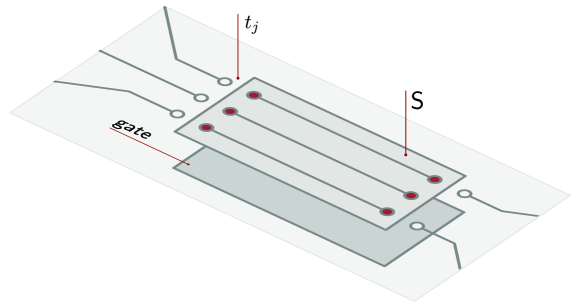
Figure 1: Multiterminal Coulomb-Majorana junction setup (schematic): $N$ helical nanowires (here $N=3$) on top of a floating mesoscopic superconductor film with charging energy $E_{c}$ are assumed to host Majorana bound states. A backgate electrode allows to gate the superconductor. Each wire holds a pair of MBSs (indicated as filled circles) associated with Majorana fermion operators $\gamma_{j}$ near the ends of proximity-coupled nanowire parts. The $M\leq 2N$ normal-conducting wire segments away from the dot (here $M=5$) act as helical Luttinger liquid leads, tunnel-coupled to the dot with amplitudes $t_{j}$. Klein factors are expressed in terms of Majorana fermions $\eta_{j}$ (open circles). For the case of $M<2N$ leads, we put one or several $t_{j}=0$.

2.1 Low-energy model: Hamiltonian

The Hamiltonian is written as $H=H_{c}+H_{t}+H_{l}$, with the dot Hamiltonian $H_{c}$, the tunneling Hamiltonian $H_{t}$, and $H_{l}$ for the normal-conducting hLL leads. Labeling the different nanowires by $\alpha=1,\ldots,N$, for each wire we assume that two spatially well separated MBSs are present, corresponding to the Majorana fermion operators $\gamma_{2\alpha-1}$ and $\gamma_{2\alpha}$, where $\gamma_{j}=\gamma_{j}^{\dagger}$ with $\{\gamma_{j},\gamma_{k}\}=\delta_{jk}$. It is convenient to define nonlocal auxiliary fermion operators $d_{\alpha}=(\gamma_{2\alpha-1}+i\gamma_{2\alpha})/\sqrt{2}$, with total number operator $\hat{n}=\sum_{\alpha}d^{\dagger}_{\alpha}d_{\alpha}$. For the parameter regime of interest, with the proximity-induced gap constituting the largest energy scale, quasiparticle excitations in the superconductor can be neglected. Hence the Majorana fermions, $\gamma_{j}$, and the Cooper pair number operator, $\hat{N}_{c}$, are the only important dot degrees of freedom. Note that $\hat{N}_{c}$ is conjugate to the condensate phase $\varphi$, i.e., we have $[\varphi,2\hat{N}_{c}]=i$ and the operator $e^{-2i\varphi}$ annihilates a Cooper pair, $N_{c}\to N_{c}-1$. Since at this stage all dot variables are zero-energy modes, the dot Hamiltonian $H_{c}$ is fully expressed by the Coulomb charging term,

$$H_{c}=E_{c}(2\hat{N}_{c}+\hat{n}-n_{g})^{2},$$ (1)

where the dimensionless offset charge $n_{g}$ can be continuously varied by a background gate voltage. Next the semi-infinite $(x>0)$ hLL leads, with tunneling contacts connecting the respective lead to the dot at $x=0$, are described by dual pairs of bosonic fields, $\phi_{j}(x)$ and $\theta_{j}(x)$, with the hLL Hamiltonian [17, 25]

$$H_{l}=\frac{v}{2\pi}\sum_{j=1}^{M}\int_{0}^{\infty}dx\left[g(\partial_{x}\phi_{j})^{2}+g^{-1}(\partial_{x}\theta_{j})^{2}\right].$$ (2)

For simplicity, we assume identical Fermi velocity $v$ and hLL parameter $g$ for all wires, with weakly repulsive interactions such that $1/2<g\leq 1$. The bosonized right- or left-moving fermion annihilation operator reads [25] $\psi_{j,R/L}(x)=a^{-1/2}\eta_{j}e^{i[\phi_{j}\pm\theta_{j}](x)}$, where $a$ is a short distance cutoff. We have also introduced a set of auxiliary Majorana fermions $\eta_{j}$, with $\{\eta_{j},\eta_{k}\}=\delta_{jk}$, to represent the ’Klein factors’ [26, 61] enforcing fermion anticommutation relations between different leads. To ensure open boundary conditions at $x=0$ in the absence of tunneling, we require $\psi_{j,L}(0)=\psi_{j,R}(0)$, thereby pinning all boson fields $\theta_{j}(0)=0$. The lead fermion operators near $x=0$ are thus written as $\Psi_{j}=a^{-1/2}\ \eta_{j}\ e^{i\phi_{j}(x=0)}$. Finally, as derived in Refs. [33, 35], the tunneling Hamiltonian connecting leads and dot reads

$$H_{t}=\sqrt{a/2}\sum_{j}t_{j}\Psi_{j}^{\dagger}\left(d_{\alpha_{j}}+(-)^{j-1}e^{-2i\varphi}d_{\alpha_{j}}^{\dagger}\right)+{\rm H.c.},$$ (3)

where $\alpha_{j}=[j/2]+1$. The term $\propto\Psi^{\dagger}d$ describes the transfer of a fermion from the dot to the lead by annihilation of a $d$-fermion. The term $\propto\Psi^{\dagger}e^{-2i\varphi}d^{\dagger}$ represents an alternative way of annihilating a dot fermion, viz. by creation of a Majorana $d$-fermion along with annihilation of a Cooper pair. Without loss of generality, the bare tunneling amplitudes are taken real and positive, $t_{j}>0$. Using Eq. (3) and the Heisenberg equation of motion, the operator

$$\hat{I}_{j}=it_{j}\sqrt{a/2}\ \Psi_{j}^{\dagger}\left(d_{\alpha_{j}}+(-)^{j-1}e^{-2i\varphi}d_{\alpha_{j}}^{\dagger}\right)+{\rm H.c.}$$ (4)

describes the current flowing from the $j$th lead towards the dot.

2.2 Real-time phase action

We next derive an action $S$ representing the above second-quantized Hamiltonian. In anticipation of our later application of the Keldysh formalism, we consider a real-time version of the theory with the action $S=S_{c}+S_{l}+S_{t}+S_{f}$,

$$S_{c}[N_{c},\varphi,d,\bar{d}] =\int dt\,\left[2N_{c}\dot{\varphi}-H_{c}(N_{c},d,\bar{d})\right],$$

$$S_{l}[\theta,\phi] =\frac{1}{\pi}\sum_{j}\int dxdt\,\partial_{t}\phi_{j}\partial_{x}\theta_{j}-\int dt\,H_{l}[\phi,\theta],$$

$$S_{t}[d,\bar{d},\eta,\phi,\varphi] =-\int dt\,H_{t}(d,\bar{d},\eta,\phi(x=0),\varphi),$$

$$S_{f}[d,\bar{d},\eta] =i\int dt\,\left(\sum_{\alpha}\bar{d}_{\alpha}\dot{d}_{\alpha}+\frac{1}{2}\sum_{j}\eta_{j}\dot{\eta}_{j}\right),$$ (5)

where $N_{c},\phi,d,\bar{d},\dots$ are the real or Grassmann valued field variables corresponding to the operators $\hat{N}_{c},\hat{\phi},d,d^{\dagger},\dots$ [24]. We start out by integrating over all those variables of the theory which do not enter in a non-trivial (non-quadratic) form. The fact that the tunneling operator couples only to the field amplitudes $\phi$ suggests to integrate over the conjugate fields $\theta_{j}(x,t)$, which yields the $\phi$-representation of the hLL action,

$$S_{l}[\phi]={g\over 2\pi v}\sum_{j}\int dxdt\,\phi_{j}\left(-\partial^{2}_{t}+v^{2}\partial_{x}^{2}\right)\phi_{j}.$$ (6)

Similarly, integration over $N_{c}$ brings the charging action $S_{c}$ into the form

$$S_{c}[\varphi,d,\bar{d}]=-2\pi Wn_{g}+\int dt\left(\frac{\dot{\varphi}^{2}}{4E_{c}}-\sum_{\alpha}\dot{\varphi}\ \bar{d}_{\alpha}d_{\alpha}\right),$$ (7)

where the presence of the integer-valued winding number $W$ reflects the discreteness of the variable $N_{c}$. The summation over the winding number $W$ encodes charge quantization due to the charging energy. We below consider only $n_{g}$ values close to an integer, where the charge state of the dot is well defined. As we show in A, the $W$ summation can then effectively be discarded.

We next remove the term $\sim\dot{\varphi}\bar{d}_{\alpha}d_{\alpha}$ by the gauge transformation $d_{\alpha}\to e^{-i\varphi}d_{\alpha}$. A side effect of this transformation is that the tunneling action $S_{t}$ now assumes a more symmetric form,

$$S_{t}[\gamma,\eta,\Phi,\varphi]=\sum_{j}t_{j}\int dt\,\hat{\sigma}_{j}\sin(\Phi_{j}+\varphi),$$ (8)

where we introduced the notation $\Phi_{j}(t)=\phi_{j}(x=0,t)$. In addition, we turned back to dot-Majorana fields, $\gamma_{2\alpha-1}=(d_{\alpha}+d_{\alpha}^{\dagger})/\sqrt{2}$ and $\gamma_{2\alpha}=-i(d_{\alpha}-d^{\dagger}_{\alpha})/\sqrt{2}$, and defined $\hat{\sigma}_{j}\equiv 2i\gamma_{j}\eta_{j}$. In essence, the Majorana fermions have been removed from the charging energy (1) through this gauge transformation, and now couple to $\varphi$ only through the tunneling term (8). Since our model assumes all direct tunneling matrix elements between different MBSs to vanish, the Majorana fermions only appear through the $M$ operators $\hat{\sigma}_{j}$. By construction, these operators do (i) commute with the system Hamiltonian, $[H,\hat{\sigma}_{j}]=0$, (ii) square to unity, $\hat{\sigma}_{j}^{2}=1$, and (iii) mutually commute, $[\hat{\sigma}_{j},\hat{\sigma}_{k}]=0$. According to (iii), all operators $\hat{\sigma}_{j}$ can be diagonalized simultaneously. According to (i) and (ii), the two possible eigenvalues $\sigma_{j}=\pm 1$ are dynamically conserved. Instead of working with the operators $\hat{\sigma}_{j}$ and the Grassmann action piece $S_{f}$ in Eq. (5) explicitly, we may therefore multiply each tunneling amplitude $\sim\sin(\Phi_{j}+\varphi)$ with an independent sign factor $\sigma_{j}=\pm 1$ and then sum over these.

Next, we note that a uniform shift, $\Phi_{j}(t)\to\Phi_{j}(t)+\pi$, only changes the sign of the respective tunneling term but leaves the remaining action invariant. The sign factor $\sigma_{j}$ can thereby be gauged away, and the perturbation series in $S_{t}$ will automatically contain only even orders in $t_{j}$. The above reasoning allows us to ignore all Grassmann fields as well as the sign factors $\sigma_{j}$. It is worth noting that this is an enormous simplification compared to other multiple Luttinger liquid tunneling contexts [61, 62, 63, 64], where the presence of Klein factors ($\eta_{j}$) leads to complicated correlations. To summarize the above steps, the effective real-time action is given by $S=S_{c}+S_{l}+S_{t}$, where

$$S_{c}[\varphi]=-\frac{1}{4E_{c}}\int dt\,\varphi\ddot{\varphi},$$ (9)

$S_{l}$ is defined in Eq. (6), and $S_{t}$ in Eq. (8). Notice that we are left with an action involving the phase-like fields $\varphi(t)$ and $\phi_{j}(x,t)$ only.

2.3 Keldysh generating functional and transport observables

In the next step, we put the real-time phase action $S$ onto a Keldysh contour and couple it to source fields, $\chi_{j}$, suitable for the calculation of transport observables [24]. To this end, let us imagine that the system can be described by an initial density matrix $\rho_{0}$ at time $t=-t_{0}/2$, where tunneling between leads and dot is assumed absent. Each of the $M$ leads thus has its own grand-canonical equilibrium density matrix with chemical potential $\mu_{j}$. We here do not discuss thermal transport and thus assume identical temperature $T$ for all leads. The initial state $\rho_{0}$ is then time-evolved under the full Hamiltonian $H$ (including tunneling) along the forward $(+)$ part of the Keldysh time contour up to $t=t_{0}/2$, followed by backward $(-)$ time evolution all the way back to $t=-t_{0}/2$. Eventually, the limit $t_{0}\to\infty$ will be taken. Using standard notation [24], we introduce time-dependent counting fields $\chi_{j}(t)$, probing the fluctuating current from the $j$th wire to the dot at time $t$. In terms of the dynamical lead fermion fields on the two Keldysh branches, $\psi_{j,\pm}(x,t)$, we gauge out the chemical potentials $\mu_{j}$ and include the counting fields $\chi_{j}$ as phase factors, $\psi_{j,\pm}(t)\to e^{i[\mu_{j}t\pm\chi_{j}(t)/2]}\psi_{j,\pm}(t),$ which therefore appear solely in the tunneling term. Note that the counting fields appear with opposite signs on the forward and backward parts of the Keldysh contour. The resulting Keldysh generating functional, with normalization $Z[0]=1$ and time-ordering operator ${\cal T}_{K}$ along the Keldysh contour,

$$Z[\chi]=\frac{{\rm Tr}\left({\cal T}_{K}e^{+iH_{-\chi}t_{0}}\rho_{0}e^{-iH_{+\chi}t_{0}}\right)}{{\rm Tr}\rho_{0}},$$ (10)

then encodes the complete information about charge transport statistics in our device.

Expectation values involving the current operators $\hat{I}_{j}$ in Eq. (4) follow as functional derivatives of $Z[\chi]$ with respect to the counting fields. For instance, the mean current flowing through the $j$th contact is given by

$$I_{j}(t)\equiv\langle\hat{I}_{j}(t)\rangle=-i\left.\frac{\delta\ln Z[\chi]}{\delta\chi_{j}(t)}\right|_{\chi=0}.$$ (11)

Under steady-state conditions, $I_{j}$ is time independent and we may define the multiterminal differential conductance tensor,

$$G_{jk}(\{\mu_{i}\})\equiv-e\frac{\partial I_{j}}{\partial\mu_{k}}.$$ (12)

The temperature dependent linear conductance tensor $G_{jk}(T)$ then follows from Eq. (12) in the near-equilibrium regime ${\rm max}|\mu_{j}-\mu_{k}|\ll T$. Similarly, the symmetrized current noise correlations are contained in [44]

$$S_{jk}(t-t^{\prime})\equiv\frac{1}{2}\left\langle\left[\Delta\hat{I}_{j}(t),\Delta\hat{I}_{k}(t^{\prime})\right]_{+}\right\rangle=-\left.\frac{\delta^{2}\ln Z[\chi]}{\delta\chi_{j}(t)\delta\chi_{k}(t^{\prime})}\right|_{\chi=0},$$ (13)

with the current fluctuation operators $\Delta\hat{I}_{j}\equiv\hat{I}_{j}-I_{j}$. Under steady state conditions, $S_{jk}$ depends only on the time difference $t-t^{\prime}$, and we switch to the Fourier-transformed noise tensor, $S_{jk}(\omega)$. Near thermal equilibrium, the linear conductance matrix $G_{jk}$ and the Johnson-Nyquist noise tensor $S_{jk}$ are linked by the fluctuation dissipation theorem [24], $S_{jk}(\omega)=\omega\coth(\omega/2T)G_{jk}$. Likewise all higher-order cumulants can in principle be extracted from the Keldysh functional (10). Fluctuation relations then impose symmetry relations for $Z[\chi]$ and thereby allow to generalize the fluctuation dissipation theorem to the nonequilibrium case. This implies a relation connecting the third cumulant and shot noise, cf. Ref. [65] and references therein.

2.4 Keldysh phase action

Following the steps in Sec. 2.2, we now represent $Z[\chi]$ as a functional integral over phase fields, $\varphi_{s}(t)$ and $\phi_{j,s}(x,t)$, for the two Keldysh contour parts $s=\pm$. The extension of the phase action $S=S_{c}+S_{l}+S_{t}$ to the Keldysh theory reads as

$$S_{c}[\varphi] =-\frac{1}{E_{c}}\int dt\,\varphi_{q}\ddot{\varphi}_{c},$$

$$S_{l}[\phi] ={2g\over\pi v}\sum_{j}\int dxdt\,\phi_{j,q}\left(-\partial^{2}_{t}+v^{2}\partial^{2}_{x}\right)\phi_{j,c},$$

$$S_{t}[\Phi,\varphi] =\sum_{s=\pm}\sum_{j}st_{j}\int dt\,\sin\left(\Phi_{j,s}+\varphi_{s}+\mu_{j}t+s\chi_{j}/2\right),$$

where $\xi_{c}=(\xi_{+}+\xi_{-})/2$ and $\xi_{q}=(\xi_{+}-\xi_{-})/2$ denote the classical and quantum components, respectively, of the field variables $\xi=(\varphi,\phi_{j})$. The Fermi distribution functions controlling the thermal occupation of lead modes at the initial time $t=-t_{0}/2$ are implicit in our notation.

Next we integrate over the Gaussian fluctuations of field modes away from the junction, $\phi(x\not=0)$. After a Fourier transformation, $S_{l}[\phi]$ gets thereby reduced to the action

$$S_{l}[\Phi]=\frac{1}{2}\sum_{j}\int{d\omega\over 2\pi}\Phi_{j}^{T}(-\omega)G^{-1}(\omega)\Phi_{j}(\omega),$$ (14)

with the Keldysh vector $\Phi\equiv\phi(0)=(\Phi_{c},\Phi_{q})^{T}$ containing the lead phase fields at $x=0$. The dissipative Green’s function matrix in Keldysh space is

$$G=\left(\begin{array}[]{cc}G_{K}&G^{+}\\ G^{-}&0\end{array}\right),\qquad G^{\pm}(\omega)=\mp{i\pi\over 2g\omega},$$ (15)

where the Keldysh component is given by $G_{K}(\omega)=(G^{+}-G^{-})(\omega)\coth(\omega/2T)$. The action $S_{l}[\Phi]$ describes Ohmic dissipation generated by the ’bath’ of lead modes kept at temperature $T$.

Finally, we remove $\varphi$ from the tunneling term by a shift $\Phi_{j}\to\Phi_{j}-\varphi$. This generates a linear coupling $\sim\varphi\Phi_{0}$ from Eq. (14), where $\Phi_{0}\equiv{1\over\sqrt{M}}\sum_{j}\Phi_{j}$. Since $\varphi$ couples only to the ’zero mode’ $\Phi_{0}$, it is beneficial to represent the field vector $\Phi\equiv\{\Phi_{j}\}$ as

$$\Phi=\Phi_{0}e_{0}+\sum_{i=1}^{M-1}\alpha_{i}\ (e_{i+1}-e_{i}),$$ (16)

with $e_{i}=(0,\dots,1,\dots,0)$ denoting a standard basis vector in lead channel space and $e_{0}\equiv{1\over\sqrt{M}}(1,\dots,1)$. The $M-1$ time-dependent fields $\alpha_{i}=(\alpha_{i,c},\alpha_{i,q})^{T}$ span the orthogonal complement of the zero mode $\Phi_{0}$. The overlap, $\Phi^{T}\Phi=\Phi_{0}^{T}\Phi_{0}-\alpha^{T}\Delta\alpha$, between the new basis vectors is described by the $(M-1)\times(M-1)$ matrix

$$\Delta=-\left(\begin{array}[]{ccccc}2&-1&0&\dots&\cr-1&2&-1&\dots&\cr&\ddots&\ddots&\ddots&\cr&\dots&-1&2&-1\cr&\dots&0&-1&2\end{array}\right).$$ (17)

The subsequent integration over $\varphi$ then transforms the Keldysh action into $S[\Phi]=S_{0}+S_{t}$, with

$$S_{0} = {1\over 2}\int{d\omega\over 2\pi}\left[\Phi_{0}^{T}(-\omega)G_{0}^{-1}(\omega)\Phi_{0}(\omega)-\alpha^{T}(-\omega)G^{-1}(\omega)\otimes\Delta\alpha(\omega)\right],$$ (18)

$$S_{t} = \sum_{s=\pm}\sum_{j=1}^{M}st_{j}\int dt\,\sin\left(\Phi_{j,s}(t)+\mu_{j}t+s\chi_{j}(t)/2\right),$$

involving only the lead boson fields at $x=0$, see Eq. (16). The zero mode Green’s function $G_{0}$ follows from

$$G^{\pm}_{0}(\omega)=\mp{i\pi\left(1\pm i\epsilon/\omega\right)\over 2g\omega},\qquad\epsilon={2gME_{c}\over\pi}.$$ (19)

The physical meaning of Eq. (19) is that at low energies, $|\omega|\ll\epsilon\sim E_{c}$, the fluctuations of the zero mode $\Phi_{0}$ become free, $G^{\pm}_{0}(\omega)\sim 1/\omega^{2}$, as a consequence of the pinning of the conjugate charge fluctuations. Note that for $E_{c}=0$, all $\Phi_{j}$ phase fields fluctuate independently, consistent with the completely decoupled leads in the resonant Andreev reflection picture [8].

3 Topological Kondo effect

In this section, the focus will be mostly on the scaling properties of the unperturbed system, and hence we set $\mu_{j}=\chi_{j}=0$ throughout. The chemical potentials and the counting fields will be restored in Sec. 4 when addressing transport observables. In a first step, we derive a Keldysh phase action describing the physics on energy scales below the charging energy.

3.1 Low-energy Keldysh phase action

Consider a perturbative expansion of $Z$ in the tunneling couplings $t_{j}$, with the effective Keldysh phase action (18). Adopting a Coulomb gas picture, we interpret the ’scattering operators’ ${\cal O}_{j,s}^{\pm}(t)=e^{\pm i\Phi_{j,s}(t)}$ as particles (’quarks’) and antiparticles living on the time axis. Each particle carries a ’flavor’ index $j=1,\ldots,M$, the Keldysh contour index $s=\pm$, and has the coupling constant (’charge’) $-it_{j}/2$. To study the properties of this interacting particle gas, we employ standard RG methods [24]. In a given RG step, all ’fast’ $\Phi(\omega)$ modes within the energy shell $\Lambda/b<|\omega|<\Lambda$ are integrated out, with rescaling parameter $b>1$ and the high-energy cutoff $\Lambda$ initially given by the proximity gap. At the end of the RG step, we rescale all energies, $\omega\to b\omega$, and thus $\Lambda$ remains invariant. In a first stage of the RG analysis, we follow the RG flow by subsequently integrating over all modes from $\omega=\Lambda$ down to $\omega=E_{c}$ [66]. For small $t_{j}$, the particle density is low and different $t_{j}$ renormalize independently. Noting from Eqs. (18) and (19) that for $\omega>E_{c}$, the zero mode $\Phi_{0}$ stays basically unaffected by the charging energy, the $t_{j}$ are relevant scaling fields with net scaling dimension $1-1/2g$ [17]. Once the RG flow has reached the energy scale $\omega=E_{c}$, the renormalized tunneling couplings are given by

$$t_{j}^{(1)}=t_{j}(\Lambda/E_{c})^{1-\frac{1}{2g}}.$$ (20)

The resulting increase of $t_{j}$ during the RG flow implies that the system approaches the resonant Andreev reflection fixed point.

However, this scenario gets modified by the charging term at energy scales $\omega<E_{c}$, where the zero mode $\Phi_{0}$ is governed by a nearly ’free’ action corresponding to $G^{\pm}_{0}(\omega)\sim 1/\omega^{2}$ in Eq. (19). Integration over the fast zero mode, see A, now generates a linear ’confinement’ potential between tunneling operators sitting on the same branch $s=\pm$ of the Keldysh contour,

$$\langle{\cal O}_{j,s}^{+}(t){\cal O}_{k,s}^{-}(t^{\prime})\rangle_{0}\simeq e^{-\frac{2E_{c}}{\pi}|t-t^{\prime}|}\ {\cal O}_{jk,s}(t),\quad{\cal O}_{jk,s}(t)=e^{i\Phi_{j,s}(t)}e^{-i\Phi_{k,s}(t)},$$ (21)

which binds particles with flavor $j$ and antiparticles with flavor $k\neq j$ together; for $k=j$, only inconsequential particle-antiparticle annihilation events occur. Notice that only the $\alpha$ part of $\Phi$ in Eq. (16), which is orthogonal to the zero mode, determines the ${\cal O}_{jk}$ operators. For low energies, $\omega\lesssim E_{c}$, the physically relevant degrees of freedom then correspond to the composite objects (’dipoles’) described by ${\cal O}_{jk}$ – within our high-energy physics analogy, these are quark-antiquark pairs (’mesons’). This indicates that the effective phase action should describe an interacting dipole gas. The dipoles have symmetric coupling strengths $\lambda_{jk}=\lambda_{kj}>0$, and therefore $S_{t}$ will be effectively given by $\cos$-terms; we put $\lambda_{jj}=0$ since particle-antiparticle annihilation processes give no dynamical contribution. Written again in terms of the phase fields $\Phi=(\Phi_{0},\alpha)$, with $S_{0}$ defined in Eq. (18), the low-energy Keldysh phase action follows as

$$S[\Phi] = S_{0}[\Phi_{0},\alpha]+S_{t}[\alpha],$$ (22)

$$S_{t} = \sum_{j,k}\sum_{s=\pm}s\lambda_{jk}\int dt\cos\left(\Phi_{j,s}-\Phi_{k,s}\right),$$

which describes the physics of our system on energy scales $\omega<E_{c}$. In physical terms, the $\lambda_{jk}$ describe the amplitude for processes where a particle is transferred from lead $j$ to lead $k$ (or back), with virtual occupation of the dot during a timespan of order $E_{c}^{-1}$. Within our low-energy approach, this corresponds to instantaneous particle transfer, dubbed ’teleportation’ in Ref. [33]. The ’bare’ $\lambda_{jk}$, defined at the high-energy cutoff scale $\omega=E_{c}$ of the effective action (22), are positive and may be estimated as [41]

$$\lambda_{jk}^{(1)}\approx\frac{t_{j}^{(1)}t_{k}^{(1)}}{E_{c}}\propto E_{c}^{-3+1/g},$$ (23)

where a factor $E_{c}^{-1}$ comes from the time integration over the particle-antiparticle separation and the $t_{j}^{(1)}$ are specified in Eq. (20).

3.2 Two-channel $\mathrm{SO}(M)$ Kondo effect

We now show that Eq. (22) naturally describes a variant of the two-channel Kondo model with $\mathrm{SO}(M)$ as the underlying symmetry group. This connection to Kondo physics has first been drawn in Ref. [39]. In the lead non-interacting limit, $g=1$, the analogies to the Kondo model can be conveniently exposed in a refermionized language. Mainly for pedagogical purposes, we briefly discuss this fermion representation now before returning to the analysis of the bosonized action for arbitrary $g$. Following standard procedures [25], we represent the fermions propagating in the now non-interacting $j$th lead in terms of the auxiliary right-moving fermion field $\psi_{j}(x)$, where ’unfolding’ of the semi-infinite wire to an infinite chiral wave guide is understood. The inter-wire coupling introduced by the dot can be represented by refermionization, i.e., by writing $e^{i\Phi_{j}}=\sqrt{a}\ \eta_{j}\psi_{j}(0)$. Notice that the Majoranas $\eta_{j}$ are not identical to the Klein-Majorana factors of the native model. Likewise, the effective fermions $\psi_{j}(x)$ differ from the original wire fermions. The effective fermion Hamiltonian equivalent to the boson representation in Eq. (22) then reads as

$$H_{f}=-iv\int_{-\infty}^{\infty}dx\sum_{j=1}^{M}\psi_{j}^{\dagger}(x)\partial_{x}\psi_{j}(x)+a\sum_{j\neq k}\lambda_{jk}\eta_{k}\eta_{j}\psi_{j}^{\dagger}(0)\psi_{k}(0).$$ (24)

For this model, the coupling constants $\lambda_{jk}$ flow under renormalization according to the one-loop RG equations [39]

$$\frac{d\lambda_{jk}}{d\ln b}=\frac{\kappa}{E_{c}}\sum_{m\neq(j,k)}\lambda_{jm}\lambda_{mk},$$ (25)

where $\kappa=\mathcal{O}(1)$ is a non-universal constant. $E_{c}$ appears as a high-energy cutoff marking the validity limit of the action (22), and hence of the refermionized model (24). For our present configuration of initially positive couplings, these equations predict a flow towards an isotropic configuration, $\lambda_{jk}\to\lambda(1-\delta_{jk})$, where $\lambda$ grows according to

$$\frac{d\lambda}{d\ln b}=\frac{\kappa(M-2)}{E_{c}}\lambda^{2}.$$ (26)

The effective Hamiltonian thus flows towards an isotropic limit,

$$H_{f}=-iv\int dx\sum_{j}\psi_{j}^{\dagger}\partial_{x}\psi_{j}+J\sum_{j\neq k}\eta_{k}\eta_{j}\psi_{j}^{\dagger}(0)\psi_{k}(0),$$ (27)

with positive coupling $J=a\lambda$. The bilinears $A_{jk}\equiv\eta_{j}\eta_{k}$ appearing in $H_{f}$ define an $\mathrm{so}(M)$ algebra. To expose the symmetry of the model in its most obvious form, we pass to a real Majorana basis for each lead channel, $\psi=\mu+i\nu$ and $\psi^{\dagger}=\mu-i\nu$, whereupon we obtain

$$H_{f}=-iv\int dx\ \mu^{T}\partial_{x}\mu-J\mu^{T}(0)\hat{A}\mu(0)+(\mu\leftrightarrow\nu)$$ (28)

with $\hat{A}=\{A_{jk}\}$. This defines a variant of the two-channel $(\mu,\nu)$ Kondo model with symmetry group $\mathrm{SO}(M)$.

3.3 Scaling equations and Kondo temperature

We now return to the Keldysh phase action (22) and allow for $g\leq 1$ again. The RG equations generalizing Eq. (25) may be obtained by standard Coulomb gas energy-shell integration, or by using the operator product expansion. The result is [41, 42]

$$\frac{d\lambda_{jk}}{d\ln b}=-\gamma\lambda_{jk}+\frac{\kappa}{E_{c}}\sum_{m\neq(j,k)}\lambda_{jm}\lambda_{mk},$$ (29)

where $\gamma\equiv g^{-1}-1>0$. The first term reflects the well-known power-law suppression of the tunneling density of states for Luttinger liquids [25], and leads to a suppression of the $\lambda_{jk}$ under the RG flow. For $M>2$ lead channels, the Kondo-like second contribution opposes this suppression. As a result of this competition, an isotropic intermediate fixed point emerges, $\lambda_{jk}=\lambda^{*}(1-\delta_{jk})$, where

$$\lambda^{*}=\frac{\gamma}{\kappa(M-2)}E_{c}.$$ (30)

Defining $\lambda_{jk}=\lambda^{*}(1-\delta_{jk})+\mu_{jk}$, the RG flow in the vicinity of this fixed point is described by the linearized equations

$${d\mu_{jk}\over d\ln b}={\gamma\over M-2}\left(-M\mu_{jk}+(1-\delta_{jk})\sum_{m=1}^{M}(\mu_{jm}+\mu_{mk})\right).$$ (31)

As detailed in B, the solution approaches the isotropic configuration

$$\mu_{jk}\sim\left\langle\mu^{(1)}\right\rangle_{\rm av}(1-\delta_{jk})b^{\gamma},$$ (32)

where the average of coupling constants over all channel indices is denoted by $\langle\mu\rangle_{\rm av}={1\over M(M-1)}\sum_{jk}\mu_{jk}$, and $\mu^{(1)}$ defines the ’bare’ couplings according to Eq. (23). Equation (32) shows that (i) anisotropic deviations in the $\lambda_{jk}$ correspond to irrelevant scaling fields, vanishing during the RG flow with the non-universal scaling dimensions specified in B, and (ii) the fixed point $\lambda^{\ast}$ in Eq. (30) is unstable. Depending on the average value of the initial deviation off the critical configuration, the flow is either to weak coupling (for $\langle\mu^{(1)}\rangle_{\rm av}<0$), or towards strong coupling ($\langle\mu^{(1)}\rangle_{\rm av}>0$). In either case, an $\mathrm{SO}(M)$-symmetric configuration will be approached.

To explore what happens in the strong coupling regime, let us consider ’bare’ couplings with $\langle\lambda^{(1)}\rangle_{\rm av}>\lambda^{*}$. Neglecting both the RG-irrelevant anisotropic contributions and the now inessential term linear in $\lambda$, Eq. (29) simplifies to the standard Kondo form (26). With the ’Kondo temperature’ defined by

$$T_{K}\approx E_{c}\exp\left(-\frac{1}{\kappa(M-2)}\frac{E_{c}}{\langle\lambda^{(1)}\rangle_{\rm av}}\right),$$ (33)

the resulting RG flow diverges at $\omega\sim T_{K}$. Clearly, the perturbative RG analysis then ceases to be valid. The physics on even lower energy scales is best discussed by switching to a dual action, as we discuss next.

3.4 Dual Keldysh phase action: Below $T_{K}$

Assuming $\langle\lambda^{(1)}\rangle_{\rm av}>\lambda^{*}$ and very low energy scales $\omega\lesssim T_{K}$, the coupling $\lambda$ effectively approaches the strong-coupling limit, where the fields $\Phi_{j}$ are confined near the minima of $S_{t}$ in Eq. (22). The dominant excitations of $\Phi=(\Phi_{0},\alpha)$ are occasional tunneling events between neighboring minima (in a slight abuse of notation referred to as ’instantons’), where $\Phi_{j,s}\to\Phi_{j,s}\pm 2\pi$. Noting that $\Phi_{0}$ does not enter the tunneling action in Eq. (22), $S_{t}=S_{t}[\alpha]$, we now perform a Hubbard-Stratonovich transformation to dual fields $(\Theta_{0},\beta)$, corresponding to the conjugate lead boson fields $\{\theta_{j}(x=0)\}$. We thus represent $S_{0}[\Phi_{0},\alpha]$ in Eq. (18) as

$$S_{0} = {1\over 2}\int{d\omega\over 2\pi}\left[\Theta^{T}_{0}(-\omega)\tilde{G}_{0}^{-1}(\omega)\Theta_{0}(\omega)-\beta^{T}(-\omega)\tilde{G}^{-1}(\omega)\otimes\Delta\beta(\omega)\right]$$

$$+ i\int{d\omega\over 2\pi}\frac{2\omega}{\pi}\left[\Phi^{T}_{0}(-\omega)\tau_{1}\Theta_{0}(\omega)+\alpha^{T}(-\omega)\tau_{1}\otimes\Delta\beta(\omega)\right],$$

with the $M-1$ time-dependent ’discrete’ variables $\beta_{i}=(\beta_{i,c},\beta_{i,q})^{T}$, and $\beta_{0}\equiv 0$. Here we used the reciprocity relation $G(\omega)=-(\pi/2\omega)^{2}\tau_{1}\tilde{G}^{-1}(\omega)\tau_{1}$, where $\tilde{G}=g^{2}G$ differs from $G$ only by the parameter exchange $g\to 1/g$ and the Pauli matrix $\tau_{1}$ acts in Keldysh space. Similar relations hold for $\tilde{G}_{0}$. The linear couplings in the second line of the transformed action indicate that the variables $(\Phi_{0},\Theta_{0})$ and $(\alpha,\Delta\beta)$ indeed form canonical pairs.

The integration over the unrestricted zero mode $\Phi_{0}$ now generates the constraint $\Theta_{0}=0$, which in physical terms implies current conservation at the dot. Turning to the nonlinear variables $\alpha$, the least costly excitations correspond to $m$-instanton configurations defined by a sequence of $2\pi$-steps occurring at times $t_{a}$, $\Phi_{i_{a},s_{a}}\to\Phi_{i_{a},s_{a}}+2\pi\sigma_{a}$, with Keldysh indices $s_{a}=\pm$ and jump directions $\sigma_{a}=\pm$ ($a=1,\ldots,m$). Taking into account the constraint $\Theta_{0}=0$, the Fourier representation of this multi-instanton profile follows from the equation

$$i\omega\Delta\alpha(\omega)=2\pi\sum_{a=1}^{m}e^{i\omega t_{a}}\sigma_{a}g_{s_{a}}\otimes(f_{i_{a}}-f_{i_{a}-1}),$$ (35)

with the Keldysh vectors $g_{\pm}={1\over 2}(1,\pm 1)^{T}$, the standard unit vectors $f_{i}$ in $(M-1)$-dimensional space, and $f_{0}\equiv 0$. Geometrically, the solutions to Eq. (35) correspond to lattice vectors of a hyper-triangular lattice embedded into the $(M-1)$-dimensional hyperplane perpendicular to the vector $e_{0}$. Substituting Eq. (35) into the action (3.4), and denoting the tunneling action for a single instanton by $iS_{\mathrm{inst}}$ [67], we obtain the multi-instanton action as $imS_{\rm inst}+S^{(m)}$ with

$$S^{(m)}=-{1\over 2}\int{d\omega\over 2\pi}\beta^{T}(-\omega)\tilde{G}^{-1}(\omega)\otimes\Delta\beta(\omega)-\sum_{a}\sigma_{a}s_{a}\left(\beta_{i_{a},s_{a}}-\beta_{i_{a}-1,s_{a}}\right)(t_{a}).$$

Integrating over the instanton times $t_{a}$, summing over $i_{a}=1,\ldots,M-1$ and the indices $\sigma_{a},s_{a}=\pm$, and taking into account all orders $m$, we finally arrive at the dual Keldysh phase action,

$$S[\beta] = -\frac{1}{2}\int\frac{d\omega}{2\pi}\beta^{T}(-\omega)\tilde{G}^{-1}(\omega)\otimes\Delta\beta(\omega)$$

$$+ y\sum_{s=\pm}s\sum_{j=1}^{M-1}\int dt\ \cos\left(\beta_{j,s}-\beta_{j-1,s}\right),$$

where the coupling constant $y\sim e^{-S_{\mathrm{inst}}}$ vanishes for $\lambda\to\infty$. We have also derived the action (3.4) by using a Villain approximation of the $\cos$-terms in Eq. (22), similar to the approach taken in Ref. [17] for the single lead ($M=1$) case.

The scaling dimension $1-\Delta_{M}$ of the nonlinear perturbation $\sim y$ in Eq. (3.4) now follows from the auxiliary relations $(\Delta^{-1})_{ii^{\prime}}=-(M-i_{>})i_{<}/M$, where $i_{</>}$ is the smaller/larger of the indices $i$ and $i^{\prime}$, and

$$\left\langle[\beta_{i}-\beta_{j}]_{s}(-\omega)\,[\beta_{i}-\beta_{j}]_{s^{\prime}}(\omega)\right\rangle_{y=0}=\tilde{G}_{ss^{\prime}}(\omega)\frac{(M-|i-j|)|i-j|}{M}.$$ (37)

First-order renormalized perturbation theory [25] then yields

$$\Delta_{M}=2g\left(1-\frac{1}{M}\right),$$ (38)

see also Refs. [42, 68, 69]. For weakly repulsive interactions, $\frac{M}{2(M-1)}<g\leq 1$, the scaling dimension $1-\Delta_{M}$ is negative and hence describes a RG-irrelevant perturbation. At higher orders in perturbation theory, additional operators $\sim\cos(\beta_{i}-\beta_{j})$ with $|i-j|>1$ may be generated. However, Eq. (37) implies that these are even more irrelevant than the perturbation in Eq. (3.4). Overall, the analysis above demonstrates the stability of the strong-coupling $\mathrm{SO}(M)$ Kondo fixed point $\lambda\to\infty$.

3.5 Discussion

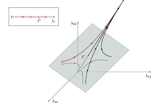
Figure 2: Illustration of the RG flow of coupling constants for $M=3$ leads. At high energy scales $\omega\gtrsim E_{c}$ (inset), tunneling couplings effectively increase as $t_{i}\sim\omega^{-1+{1\over 2g}}$ during the first stage of the RG flow. Their terminal value, reached at $\omega\sim E_{c}$, then determines the initial ’bare’ dipole couplings, $\lambda^{(1)}_{jk}\propto E_{c}^{-3+1/g}$, see Eq. (23). These dipole couplings enter the effective low-energy action (22), and constitute the scaling variables during the second stage of the RG flow (where $\omega\lesssim E_{c}$). Depending on whether the average value $\langle\lambda^{(1)}\rangle_{\rm av}$ is larger or smaller than the repulsive fixed point $\lambda^{\ast}\propto E_{c}$, the system now flows either to strong coupling ($\lambda\to\infty$), or to the decoupled fixed point $\lambda=0$; cf. the trajectories starting with $\square$ and $\circ$ symbols, resp. Inter-channel deviations in the coupling strengths are irrelevant and scale to zero with non-universal scaling dimensions.

Let us now summarize the full picture emerging for the scaling of the coupling constants all the way from high energy scales (comparable to the bandwidth $\Lambda$ set by the proximity gap) down to the actually probed scale set by temperature or applied voltages; for illustration, see Fig. 2. Lowering the energy scale from $\omega=\Lambda$, the direct single-particle tunneling couplings $t_{j}$ grow independently. This growth will stop at the energy scale $\omega\sim E_{c}$, where confinement sets in. The weaker the charging energy $E_{c}$, the larger the coupling constants may become before this flow stops, see Eq. (20). For $\omega\lesssim E_{c}$, the theory is instead governed by a system of ’dipoles’ coupled at strength $\lambda_{jk}$, with the ’bare’ values $\lambda^{(1)}_{jk}$ in Eq. (23). Everything now depends on whether the ’bare’ coupling strength averaged over all configurations, $\langle\lambda^{(1)}\rangle_{\rm av}$, is larger or smaller than the unstable isotropic fixed point $\lambda^{\ast}$ in Eq. (30). For $\langle\lambda^{(1)}\rangle_{\rm av}>\lambda^{*}$, the RG flow proceeds towards a strong-coupling $\mathrm{SO}(M)$-symmetric fixed point, $\lambda_{j\neq k}=\lambda\to\infty$. Deviations in the strength between different $\lambda_{jk}$ scale to zero, where the details of the flow are discussed in B. Note that in conventional multi-channel Kondo proposals, anisotropy is a relevant perturbation and easily destabilizes the Kondo fixed point [25]. In contrast, the present system is robust in that it flows towards an isotropic configuration. If the charging energy is too large for $\langle\lambda^{(1)}\rangle_{\rm av}$ to reach $\lambda^{\ast}$, the flow will be towards an equally isotropic configuration with $\lambda\to 0$ [41]. In this limit, we recover the conventional Luttinger liquid junction behavior [61, 62, 63, 64], where all leads effectively decouple from the dot at very low energies.

4 Transport observables

In this section, we address the differential conductance tensor, $G_{jk}$, defined in Eq. (12), and the shot noise tensor, $S_{jk}=S_{jk}(\omega=0,T=0)$, defined in Eq. (13). Within our phase action approach, $Z[\chi]$ has been represented as Keldysh functional integral over the phase fields $\Phi=(\Phi_{0},\alpha)$, or the dual $\beta$ variables. For large $E_{c}$ and $g<1$, the system flows towards the decoupled fixed point $\lambda=0$, where perturbative expansion in $\lambda_{jk}$ with the action (22) yields the low-energy dependence of all transport observables. This decoupled fixed point has been studied in depth before [25, 63] and implies a Luttinger power-law suppression of the linear conductance, $G_{jk}\sim T^{2/g-2}$, at low temperatures. The shot noise near the decoupled fixed point has also been analyzed [70].

We here focus on the case of intermediate charging energy $E_{c}$ with $M>2$ leads, where the RG flow is towards the strong-coupling Kondo fixed point as long as $\Delta_{M}>1$, with $\Delta_{M}$ in Eq. (38). Using the energy scale $\Omega={\rm max}(|\mu_{j}-\mu_{k}|,T)$, we may now distinguish three different regimes. First, in the high energy regime, $\Omega>E_{c}$, the charging energy does not significantly affect the noninteracting resonant Andreev reflection scenario. The Keldysh phase action is then given by Eq. (18) with $G_{0}\to G$, and it is straightforward to derive the temperature dependence of the linear conductance, $G_{jk}\sim T^{-2+1/g}$. Putting $g=1$, the well known $1/T$ scaling of the zero bias anomaly peak conductance at high temperatures is recovered [4]. Similarly, the shot noise here corresponds to the Fano factor $F=2$ found in the resonant Andreev reflection regime [15].

Proceeding to lower energies, $\Omega<E_{c}$, the charging energy implies dipole formation as described by the action $S[\Phi]=S_{0}+S_{t}$ in Eq. (22). The chemical potentials and the counting fields can be included by shifting $\Phi_{j}(t)\to\Phi_{j}(t)+(\tilde{\mu}_{j}t,\tilde{\chi}_{j}(t)/2)^{T}$ in $S_{t}$. Gauge invariance implies that these appear only through the quantities

$$\tilde{\mu}_{j}=\mu_{j}-\frac{1}{M}\sum_{k=1}^{M}\mu_{k},\quad\tilde{\chi}_{j}=\chi_{j}-\frac{1}{M}\sum_{k=1}^{M}\chi_{k}.$$ (39)

The regime $T_{K}<\Omega<E_{c}$ could then be analyzed by perturbation theory in the $\lambda_{jk}$.

However, we here only discuss the most interesting low-energy regime, $\Omega<T_{K}$, where the dual Keldysh action $S[\beta]$ in Eq. (3.4) applies. The chemical potentials and counting fields then yield the additional action piece

$$S_{V}[\beta]=-\frac{2}{\pi}\sum_{j=1}^{M}\int dt\ V^{T}_{j}\tau_{1}\left(\beta_{j}-\beta_{j-1}\right),\quad V_{j}(t)=\left(\begin{array}[]{c}\tilde{\mu}_{j}\\ \frac{1}{2}\dot{\tilde{\chi}}_{j}\end{array}\right),$$ (40)

with the Pauli matrix $\tau_{1}$ in Keldysh space. By using $\tilde{\mu}_{j}$ and $\tilde{\chi}_{j}$, current conservation is automatically maintained, and thus the conductance sum rule $\sum_{j=1}^{M}G_{jk}=0$ always holds. Since the nonlinear perturbation $\sim y$ in Eq. (3.4) is RG-irrelevant, the transport observables for $\Omega<T_{K}$ follow by expanding $\ln Z[\chi]=\sum_{n=0}^{\infty}\ln Z^{(n)}[\chi]$ in powers of $y$, where we report only on the lowest two nontrivial orders ($n=0,2$). The unitary limit behavior follows by putting $y=0$ in $S[\beta]$. Performing the remaining Gaussian field integration over $\beta$, we find

$$\ln Z^{(0)}[\chi]=-\frac{2i}{\pi^{2}}\int\frac{d\omega}{2\pi}V^{T}(-\omega)\tau_{1}\tilde{G}(\omega)\tau_{1}V(\omega).$$ (41)

Some algebra gives for the second-order contribution the result

$$\ln Z^{(2)}[\chi] = \frac{y^{2}}{2}\sum_{j=1}^{M}\sum_{\sigma=\pm}\int dt_{1}dt_{2}e^{-2J(t_{1}-t_{2})-2i\sigma g\tilde{\mu}_{j}(t_{1}-t_{2})}\times$$

$$\times \prod_{r=1,2}\sin\left[K(t_{1}-t_{2})+g\sigma\tilde{\chi}_{j}(t_{r})\right],$$

where the lead ’bath’ correlation function is given by

$$J(t)-iK(t)=\Delta_{M}\int_{0}^{E_{c}}\frac{d\omega}{\omega}\left\{[1-\cos(\omega t)]\coth(\omega/2T)-i\sin(\omega t)\right\}.$$ (43)

The linear conductance tensor then follows from Eq. (12), see also Ref. [42],

$$G_{jk}(T\ll T_{K})=\frac{2ge^{2}}{h}\left(\delta_{jk}-\frac{1}{M}\right)\left[1-c_{0}(T/T_{K})^{2\Delta_{M}-2}+\cdots\right],$$ (44)

where $c_{0}={\cal O}(1)$ and

$$T_{K}\equiv\left(\frac{\Gamma(2\Delta_{M})E^{2}_{c}}{2\pi g^{2}y^{2}}\right)^{1/2(\Delta_{M}-1)}\frac{E_{c}}{2g},$$ (45)

with $\Gamma$ denoting the Gamma function. Equation (45) defines the Kondo temperature from the perspective of the strong coupling theory. In Eq. (33), we had identified $T_{K}$ as the low energy scale where the coupling constants of the weak coupling theory diverge. At lower energies, we are operating in the realm of the dual strong coupling theory discussed presently. The validity regime of the latter is limited by a high energy scale $\sim T_{K}$, where the corrections due to infrared irrelevant nonlinearities remain strong enough to produce $\mathcal{O}(1)$ corrections to the asymptotic Gaussian fixed point theory. Our perturbative analysis identifies this scale as in Eq. (45), which may be regarded as a definition of $T_{K}$ in terms of the dual coupling constant.

Equation (44) describes an isotropically hybridized multiterminal junction. Following standard arguments [6, 71, 72, 73], when the one-dimensional nanowire ’leads’ are eventually connected to wide bulk reservoirs, the prefactor $g$ in Eq. (44) is replaced by the Fermi liquid value of the reservoirs, $g\to 1$. The $T^{2\Delta_{M}-2}$ power-law corrections to the unitary limit should be contrasted to the corresponding $\sqrt{T}$ temperature dependence for the two-channel $\mathrm{SU}(2)$ Kondo case [60].

In the zero temperature limit, Eq. (43) yields $J(t)\simeq\Delta_{M}\ln(E_{c}|t|)$ and $K(t)\simeq\frac{\pi}{2}\Delta_{M}\ {\rm sgn}(t)$. It is then straightforward to establish that the currents,

$$I_{j}=\frac{2ge^{2}}{h}\sum_{k=1}^{M}\left(\delta_{jk}-\frac{1}{M}\right)\mu_{k}+I^{(2)}_{j}+\cdots,$$ (46)

receive the ’backscattering’ corrections

$$I_{j}^{(2)}=-\frac{e}{\hbar}\sum_{k=1}^{M}\left|\frac{\tilde{\mu}_{k}}{T_{K}}\right|^{2\Delta_{M}-2}\left(\delta_{jk}-\frac{1}{M}\right)\tilde{\mu}_{k}.$$ (47)

Turning to the $T=0$ shot noise tensor, we find that a finite contribution may arise only in order $y^{2}$. This shot noise suppression in the unitary limit is a direct consequence of the ’free’ zero mode dynamics. Note that also the cross-correlations between different terminals are suppressed, despite of the current partitioning implied by Eq. (44). Equation (4) yields the shot noise tensor

$$S_{jk}=-\frac{2ge^{2}}{\hbar}\sum_{l=1}^{M}\left(\delta_{jl}-\frac{1}{M}\right)\left(\delta_{kl}-\frac{1}{M}\right)\left|\frac{\tilde{\mu}_{l}}{T_{K}}\right|^{2\Delta_{M}-2}|\tilde{\mu}_{l}|.$$ (48)

To define the Fano factors in this multiterminal setting, it is customary [74] to compare $S_{jk}$ to the backscattered currents (47). Writing $\tilde{\mu}_{j}\sim V$ with an overall ’voltage’ scale, we observe that the Fano factors are again universal (independent of $V$ or $T_{K}$). Taking, for instance, $\mu_{1}=V$ and $\mu_{j>1}=-V/(M-1)$, the Fano factor pertaining to the first lead is

$$F_{1}=\frac{S_{11}}{eI^{(2)}_{1}}=\frac{2g}{M}\frac{(M-1)^{2\Delta_{M}}+1}{(M-1)^{2\Delta_{M}-1}+1}.$$

For $M\gg 1$, we recover the effectively noninteracting Fano factor $F=2$ predicted by the resonant Andreev reflection picture [15]. Shot noise measurements could thus probe the noninteger scaling dimensions $\Delta_{M}$ associated with non-Fermi liquid behavior in this two-channel $\mathrm{SO}(M)$ Kondo problem.

5 Concluding remarks

In this paper we have analyzed a multiterminal Coulomb-Majorana junction, where the junction is formed by a mesoscopic superconductor containing Majorana bound states due to the presence of helical nanowires. For $M$ attached leads, a two-channel Kondo model with symmetry group $\mathrm{SO}(M)$ emerges when the charging energy of the ’dot’ is finite. Salient features of this Kondo effect include dynamically generated universality — no fine tuning of coupling constants is required to establish the underlying $\mathrm{SO}(M)$ symmetry —, and non-Fermi liquid scaling in the vicinity of the strong coupling fixed point. It stands to reason that this scaling might become observable by transport measurements.

We close by re-emphasizing two assumptions crucial to the physics discussed here. First, the relevant energy scales (e.g., temperature, applied voltages, or the charging energy) should be below the superconducting gap to avoid quasiparticle excitations. Second, direct tunneling processes between Majorana bound states are assumed absent. This issue is probably important for presently discussed implementations, where the typical MBS size is believed to be of the order of several 100 nm. Direct tunneling is an RG-relevant perturbation, like the magnetic Zeeman field in the usual Kondo problem, and is expected to strongly affect the Kondo physics reported here. Since tunneling spoils the usefulness of our Klein-Majorana fusion trick, a modified theoretical approach would also be necessary to describe this situation. We hope that future work will address this challenge, as well as the experimental realization of this proposal.

Appendix A Winding number summation

Here we address the summation over the integer winding numbers $W$ appearing in Eq. (7). For simplicity, we switch to the imaginary time ($\tau$) version of the theory. Taking into account the tunneling action (8) and integrating over the bulk lead modes, the partition sum has the following functional integral representation over the boundary boson fields $\Phi_{j}(\tau)$ and the condensate phase field $\varphi(\tau)$:

$$Z = \sum_{W=-\infty}^{\infty}e^{2\pi in_{g}W}\int D{\varphi}e^{-\frac{1}{4E_{c}}\int d\tau\dot{\varphi}^{2}}\int D\Phi e^{-S_{l}[\Phi]-S_{t}[\Phi,\varphi]},$$

$$S_{l} = \frac{Tg}{2\pi}\sum_{j=1}^{M}\sum_{\omega}|\omega||\Phi_{j}(\omega)|^{2},\quad S_{t}=\sum_{j}t_{j}\int d\tau\sin(\Phi_{j}+\varphi),$$

with $\varphi(\tau+1/T)=\varphi(\tau)+2\pi W$ and bosonic Matsubara frequencies $\omega$. Writing $\varphi(\tau)=\tilde{\varphi}(\tau)+2\pi WT\tau$, shifting $\Phi_{j}\to\Phi_{j}-\tilde{\varphi}$, and performing the Gaussian functional integral over $\tilde{\varphi}$, we obtain

$$Z = \sum_{W}e^{2\pi in_{g}W-\frac{\pi^{2}T}{E_{c}}W^{2}}Z^{(W)},\quad Z^{(W)}=\int D{\Phi}e^{-S_{l}[\Phi]-S^{(W)}_{t}[\Phi]},$$

$$S_{l} = \frac{Tg}{2\pi}\sum_{\omega}|\omega|\left(\frac{1}{1+\epsilon/|\omega|}|\Phi_{0}(\omega)|^{2}-\alpha^{T}(-\omega)\Delta\alpha(\omega)\right),$$

$$S_{t}^{(W)} = \sum_{j}t_{j}\int d\tau\sin(\Phi_{j}+2\pi WT\tau),$$

with $\epsilon\sim E_{c}$ in Eq. (19). In the dissipative action $S_{l}[\Phi=(\Phi_{0},\alpha)]$, the zero mode $\Phi_{0}=\sum_{j}\Phi_{j}/\sqrt{M}$ has been isolated, where $(\alpha_{1},\ldots,\alpha_{M-1})$ is the orthogonal complement, see Eq. (16). The matrix $\Delta$ has been specified in Eq. (17).

Figure 3: Main panel: Confinement potential $\nu(\tau)$ defined in Eq. (49) for $E_{c}/T=50$ and various values of the gate voltage parameter $n_{g}$. Inset: Partition function $Z_{0}(n_{g})$ of the isolated dot as a function of $n_{g}$, again for $E_{c}/T=50$.

We are now ready to integrate over the ’free’ zero mode $\Phi_{0}$, which yields $Z^{(W)}=\int D\alpha e^{-S_{l}[\alpha]-S^{(W)}_{t}[\alpha]}$ with

$$S^{(W)}_{t} = -\frac{1}{4}\sum_{j\neq k}t_{j}t_{k}\int d\tau_{1}d\tau_{2}\ \nu^{(W)}(\tau_{1}-\tau_{2})\cos[\Phi_{j}(\tau_{1})-\Phi_{k}(\tau_{2})],$$

$$\nu^{(W)}(\tau) = e^{-2E_{c}|\tau|/\pi}\cos(2\pi WT\tau).$$

Summation over $W$ writes the partition sum as $Z=\int D\alpha e^{-S_{l}[\alpha]-S_{t}[\alpha]}$, where second-order cumulant expansion in the tunneling amplitudes $t_{j}$ gives $S_{t}=\langle S_{t}^{(W)}\rangle_{W}$. In effect, the kernel $\nu^{(W)}$ is thereby replaced by $\nu(\tau)=\langle\nu^{(W)}(\tau)\rangle_{W}$. Explicitly, we find the ’dipole confinement’ kernel

$$\nu(\tau)=e^{-2E_{c}|\tau|/\pi}\frac{\vartheta(n_{g}+T\tau,i\pi T/E_{c})+\vartheta(n_{g}-T\tau,i\pi T/E_{c})}{2Z_{0}(n_{g})},$$ (49)

where $\vartheta$ is the Jacobi theta function, and $Z_{0}(n_{g})=\vartheta(n_{g},i\pi T/E_{c})$ is the partition function of the isolated dot; note that $Z_{0}(n_{g}+1)=Z_{0}(n_{g})$. The kernel (49) is shown for various values of $n_{g}$ in Fig. 3. For nearly integer $n_{g}$, the winding number average has little effect on the confinement kernel, which is well approximated by retaining only the $W=0$ sector, $\nu(\tau)\approx\nu^{(W=0)}(\tau)$. Only when $n_{g}$ is close to half-integer values, dipole formation – which is induced by an exponential decay of the kernel $\nu(\tau)$ – will be disrupted. We here assume $n_{g}$ to stay away from half-integer values, such that winding number effects play no important role. In the main text, we then discuss only the $W=0$ sector and approximate Eq. (49) by Eq. (21).

Appendix B Scaling dimensions

In order to solve Eq. (31), we introduce the discrete Fourier representation

$$\tilde{\mu}_{qp}=\sum_{jk}\mu_{jk}\,e^{i(jq+kp)},\qquad\mu_{jk}={1\over M^{2}}\sum_{qp}\tilde{\mu}_{qp}\,e^{-i(jq+kp)},$$

where $q,p\in\{0,\dots,M-1\}(2\pi/M)\ \mathrm{mod}(2\pi)$, and the symmetry $\mu_{jk}=\mu_{kj}$ translates to $\tilde{\mu}_{qp}=\tilde{\mu}_{pq}$. Using this representation, we obtain

$${d\tilde{\mu}_{qp}\over d\ln b}={\gamma M\over M-2}\left(-\tilde{\mu}_{qp}+\delta_{p,0}\tilde{\mu}_{q0}+\delta_{q,0}\tilde{\mu}_{0p}-{1\over M}(\tilde{\mu}_{(p+q)0}+\tilde{\mu}_{0(p+q)})\right).$$

This implies that

$$q,p\not=0 ,\qquad{d\tilde{\mu}_{qp}\over d\ln b}=-{\gamma\over M-2}\left(M\tilde{\mu}_{qp}+\tilde{\mu}_{(p+q)0}+\tilde{\mu}_{0(p+q)}\right),$$

$$q\not=0 ,\qquad{d\tilde{\mu}_{q0}\over d\ln b}=-{2\gamma\over M-2}\tilde{\mu}_{q0},$$

$$\qquad{d\tilde{\mu}_{00}\over d\ln b}=\gamma\tilde{\mu}_{00}.$$

According to these equations, (i) the Fourier mode $\tilde{\mu}_{00}$ grows as $\tilde{\mu}_{00}=\tilde{\mu}^{(1)}_{00}b^{\gamma}$, where $\tilde{\mu}^{(1)}_{qp}$ follows from the ’bare’ coupling constants. (ii) Generic modes $\tilde{\mu}_{qp}$ decay with the dimensions specified above, with the exception (iii) of modes $\mu_{q,2\pi-q}$. These modes exhibit the RG scaling $\tilde{\mu}_{q,2\pi-q}\sim-{1\over M-1}\tilde{\mu}^{(1)}_{00}b^{\gamma}$. Substituting this result back into the inverse Fourier representation, and using $\tilde{\mu}_{00}^{(1)}=\sum_{jk}\mu_{jk}^{(1)}$, we obtain Eq. (32).

References

References

- [1] Hasan M Z and Kane C L 2010 Rev. Mod. Phys. 82 3045
- [2] Qi X L and Zhang S C 2011 Rev. Mod. Phys. 83 1057
- [3] Beenakker C W J 2013 Annu. Rev. Condens. Matter Phys. 4 113
- [4] Alicea J 2012 Rep. Prog. Phys. 75 076501
- [5] Leijnse M and Flensberg K 2012 Semicond. Sci. Techn. 27 124003
- [6] Lutchyn R M, Sau J D and Das Sarma S 2010 Phys. Rev. Lett. 105 077001
- [7] Oreg Y, Refael G and von Oppen F 2010 Phys. Rev. Lett. 105 177002
- [8] Bolech C J and Demler E 2007 Phys. Rev. Lett. 98 237002
- [9] Semenoff G W and Sodano P 2007 J. Phys. B 40 1479
- [10] Nilsson J, Akhmerov A R and Beenakker C W J 2008 Phys. Rev. Lett. 101 120403
- [11] Law K T, Lee P A and Ng T K 2009 Phys. Rev. Lett. 103 237001
- [12] Flensberg K 2010 Phys. Rev. B 2010 83 180516(R)
- [13] Wimmer M, Akhmerov A R, Dahlhaus J P and Beenakker C W J 2010 New J. Phys. 13 053016
- [14] Chung S B, Qi X L, Maciejko J and Zhang S C 2011 Phys. Rev. B 83 100512(R)
- [15] Golub A and Horowitz B 2011 Phys. Rev. B 83 153415(R)
- [16] Bose S and Sodano P 2011 New J. Phys. 13 085002
- [17] Fidkowski L, Alicea J, Lindner N H, Lutchyn R M and Fisher M P A 2012 Phys. Rev. B 85 245121
- [18] Lutchyn R M and Skrabacz J B 2013 Phys. Rev. B 88 024511
- [19] Mourik V, Zuo K, Frolov S M, Plissard S R, Bakkers E P A M and Kouwenhoven L P 2012 Science 336 1003
- [20] Rokhinson L, Liu X and Furdyna J 2012 Nature Physics 8 795
- [21] Deng M T, Yu C L, Huang G Y, Larsson M, Caroff P and Xu H Q 2012 Nano Lett. 12 6414
- [22] Das A, Ronen Y, Most Y, Oreg Y, Heiblum M and Shtrikman H 2012 Nature Phys. 8 887
- [23] Churchill H O H, Fatemi V, Grove-Rasmussen K, Deng M T, Caroff P, Xu H Q and Marcus C M 2013 Phys. Rev. B 87 241401(R)
- [24] Altland A and Simons B D 2010 Condensed Matter Field Theory (Cambridge University Press, Cambridge, UK), 2nd edition
- [25] Gogolin A O, Nersesyan A A and Tsvelik A M 1998 Bosonization and strongly correlated systems (Cambridge University Press, Cambridge, UK)
- [26] von Delft J and Schoeller H 1998 Ann. Phys. (Leipzig) 7 225
- [27] Gangadharaiah S, Braunecker B, Simon P and Loss D 2011 Phys. Rev. Lett. 107 036801
- [28] Stoudenmire E M, Alicea J, Starykh O A and Fisher M P A 2011 Phys. Rev. B 84 014503
- [29] Sela E, Altland A and Rosch A 2011 Phys. Rev. B 84 085114
- [30] Alicea J, Oreg Y, Refael G, von Oppen F and Fisher M P A 2011 Nature Physics 7 412
- [31] Halperin B I, Oreg Y, Stern A, Refael G, Alicea J and von Oppen F 2012 Phys. Rev. B 85 144501
- [32] Zazunov A, Sodano P and Egger 2013 New J. Phys. 15 035033
- [33] Fu L 2010 Phys. Rev. Lett. 104 056402
- [34] Xu C and Fu L 2010 Phys. Rev. B 81 134435
- [35] Zazunov A, Levy Yeyati A and Egger R 2011 Phys. Rev. B 84 165440
- [36] van Heck B, Hassler F, Akhmerov A R and Beenakker C W J 2011 Phys. Rev. B 84 180502(R)
- [37] Hützen R, Zazunov A, Braunecker B, Levy Yeyati A and Egger R 2012 Phys. Rev. Lett. 109 166403
- [38] van Heck B, Akhmerov A R, Hassler F, Burrello M and Beenakker C W J 2012 New J. Phys. 14 035019
- [39] Béri B and Cooper N R 2012 Phys. Rev. Lett. 109 156803
- [40] Tsvelik A M 2013 Phys. Rev. Lett. 110 147202
- [41] Altland A and Egger R 2013 Phys. Rev. Lett. 110 196401
- [42] Béri B 2013 Phys. Rev. Lett. 110 216803
- [43] Crampé N and Trombettoni A 2013 Nucl. Phys. B 871 [FS] 526
- [44] Blanter Ya M and Büttiker M 2000 Phys. Reports 336 1
- [45] Sukhorukov E V, Burkard G and Loss D 2001 Phys. Rev. B 63 125315
- [46] Thielmann A, Hettler M H, König J and Schön G 2005 Phys. Rev. Lett. 95 146806
- [47] Meir Y and Golub A 2002 Phys. Rev. Lett. 88 116802
- [48] Sela E, Oreg Y, von Oppen F and Koch J 2006 Phys. Rev. Lett. 97 086601
- [49] Gogolin A O and Komnik A 2006 Phys. Rev. Lett. 97 016602
- [50] Golub A 2006 Phys. Rev. B 73 233310
- [51] Zarchin O, Zaffalon M, Heiblum M, Mahalu D and Umansky V 2008 Phys. Rev. B 77 241303(R)
- [52] Yamauchi Y, Sekiguchi K, Chida K, Arakawa T, Nakamura S, Kobayashi K, Ono T, Fujii T and Sakano R 2010 Phys. Rev. Lett. 106 176601
- [53] Golub A 2007 Phys. Rev. B 75 155313
- [54] Mora C 2009 Phys. Rev. B 80 125304
- [55] Mora C, Vitushinsky P, Leyronas X, Clerk A A and Le Hur K 2009 Phys. Rev. B 80 155322
- [56] Sakano R, Fujii T and Oguri A 2011 Phys. Rev. B 83 075440
- [57] Sakano R, Nishikawa Y, Oguri A, Hewson A C and Tarucha S 2012 Phys. Rev. Lett. 108 266401
- [58] Sasaki S, Amaha S, Asakawa N, Eto M and Tarucha S 2004 Phys. Rev. Lett. 93 017205
- [59] Delattre T, Feuillet-Palma C, Herrmann L G, Morfin P, Berroir J M, Feve G, Placais B, Glattli D C, Choi M S, Mora C and Kontos T 2009 Nature Phys. 5 208
- [60] Potok R M, Rau I G, Shtrikman H, Oreg Y and Goldhaber-Gordon D 2007 Nature 446 167
- [61] Oshikawa M, Chamon C and Affleck I 2006 J. Stat. Mech. Theor. Exp. 2006 P02008
- [62] Nayak C, Fisher M P A, Ludwig A W W and Lin H H 1999 Phys. Rev. B 59 15694
- [63] Chen S, Trauzettel B and Egger R 2002 Phys. Rev. Lett. 89 226404
- [64] Altland A, Gefen Y and Rosenow B 2012 Phys. Rev. Lett. 108 136401
- [65] Altland A, De Martino A, Egger R and Narozhny B 2010 Phys. Rev. B 82 115323
- [66] While the crossover scale in Eq. (18) is given by , confinement sets in for , see Eq. (21). Since for , this may leave room for an intermediate regime. However, this will not qualitatively affect the results discussed here.
- [67] Note that the real-time tunneling action of a single instanton is purely imaginary, see Weiss U 2012 Quantum Dissipative Systems, 4th edition (World Scientific, Singapore)
- [68] Yi H and Kane C L 1998 Phys. Rev. B 57 R5579
- [69] Yi H 2002 Phys. Rev. B 65 195101
- [70] Trauzettel B, Egger R and Grabert H 2002 Phys. Rev. Lett. 88 116401
- [71] Maslov D L and Stone M 1995 Phys. Rev. B 52 R5539
- [72] Safi I and Schulz H J 1995 Phys. Rev. B 52 R17040
- [73] Ponomarenko V 1995 Phys. Rev. B 52 R8666
- [74] Sánchez D and López R 2005 Phys. Rev. B 71 035315