Connector algebras for C/E and P/T nets’ interactions

Abstract.

A quite flourishing research thread in the recent literature on component-based systems is concerned with the algebraic properties of different classes of connectors. In a recent paper, an algebra of stateless connectors was presented that consists of five kinds of basic connectors, namely symmetry, synchronization, mutual exclusion, hiding and inaction, plus their duals, and it was shown how they can be freely composed in series and in parallel to model sophisticated “glues”. In this paper we explore the expressiveness of stateful connectors obtained by adding one-place buffers or unbounded buffers to the stateless connectors. The main results are: i) we show how different classes of connectors exactly correspond to suitable classes of Petri nets equipped with compositional interfaces, called nets with boundaries; ii) we show that the difference between strong and weak semantics in stateful connectors is reflected in the semantics of nets with boundaries by moving from the classic step semantics (strong case) to a novel banking semantics (weak case), where a step can be executed by taking some “debit” tokens to be given back during the same step; iii) we show that the corresponding bisimilarities are congruences (w.r.t. composition of connectors in series and in parallel); iv) we show that suitable monoidality laws, like those arising when representing stateful connectors in the tile model, can nicely capture concurrency (in the sense of step semantics) aspects; and v) as a side result, we provide a basic algebra, with a finite set of symbols, out of which we can compose all P/T nets with boundaries, fulfilling a long standing quest.

1. Introduction

A successful and widely adopted approach to modern software architectures is the so-called component-based approach [42]. At its core, it is centred around three main kinds of elements: processing elements (also called components), data elements and connecting elements (also called connectors). The main idea is to assemble heterogeneous and separately developed components that exchange data items via their programming interfaces by synthesising the appropriate “glue” code, i.e., by linking components via connectors. In this sense, connectors must take care of all those aspects that lie outside of the scopes of individual components and for which the operating infrastructure is held responsible. Typically, components and connectors are made available and assembled off-the-shelf. To favour their re-usability, their semantic properties, including requirements and offered guarantees must be unambiguously specified. Thus, connectors are first class entities and assessing rigorous mathematical theories for them is of crucial relevance for the analysis of component-based systems.

Connectors can live at different levels of abstraction (architecture, software, processes) and several kinds of connectors have been studied in the literature [1, 26, 14, 11, 6]. Here we focus on the approach initiated in [13] and continued in [14], where a basic algebra of stateless connectors was presented. It consists of five kinds of basic connectors (plus their duals), namely symmetry, synchronisation, mutual exclusion, hiding and inaction. The connectors can be composed in series or in parallel and the resulting circuits are equipped with a normal form axiomatization. These circuits are quite expressive: they can model the coordination aspects of the architectural design language CommUnity [26] and, using in addition a simple 1-state buffer, the classic set of “channels” provided by the coordination language Reo [1] (see [2]).

In [49, 15] the aforementioned stateless connectors were presented in process algebra form and given a subtly different operational semantics, emphasising the role of the algebra of labels, in particular with a label $0$ meaning inaction [49] and, in [15] with a monoidal structure (of which $0$ is the identity). Moreover, they were extended with certain simple buffer components: one-place buffers in [49] and unbounded buffers in [15]. In both cases close semantic correspondences were shown to exist with certain versions of Petri nets, called nets with boundaries. They come equipped with left- and right-interfaces to be exploited for composition. Interfaces are just plain lists of ports (not just shared places) that are used to coordinate the firing of net transitions with the surrounding environment.

Petri nets [45] are frequently used both in theoretical and applied research to specify systems and visualise their behaviour. On the other hand, process algebras are built around the principle of compositionality: their semantics is given structurally so that the behaviour of the whole system is a function of the behaviour of its subsystems. As a consequence, the two are associated with different modelling methodologies and reasoning techniques. This paper improves and extends the results of [49, 15], which were initial and fragmented in the two aforementioned papers. Our results bridge the gap between the Petri net theory and process algebra by showing very close semantic correspondence between a family of process algebras based on connectors on the one hand and a family of nets with boundaries on the other. Still, we want to stress out the fact that our operators for composition of systems and interaction are fundamentally different to those traditionally considered by process algebraists.

As usual, in the case of Condition/Event systems (C/E nets), each place can contain a token at most, and transitions compete both for resources in their presets and their postsets—two transitions that produce a token at the same place cannot fire together. In the case of Place/Transition systems (P/T nets), each place can contain an unbounded number of tokens, arcs between places and transitions are weighted, with the weights defining how many tokens are produced/consumed in each place by a single firing of the transition, and the firing of a transition is allowed also when some tokens are already present in its post-set. In both cases, ports of the interface can be connected to transitions to account for the interactions with the environment when a transition fires.

We focus on the step semantics, where (multi)sets of transitions can fire at the same time. In the case of P/T nets we consider two different kinds of semantics: an ordinary firing semantics in which a concurrently enabled multiset of transitions can fire together, as well as a second semantics in which any multiset of transitions can fire together when the number of tokens consumed from each place does not exceed the number of tokens available at the beginning plus those that are produced. This means that not all of the transitions are necessarily enabled at the start: by analogy with the bank system, we can consider that the multiset of transitions is enabled by each place in the net initially taking some “loan” tokens that are given back after the firing. Because of this analogy we will refer to this semantics as the banking semantics. The weak semantics resembles the firing condition for P/T nets with a/sync places proposed in [32, 33, 34], in which tokens in a/sync places can be produced and consumed at the same execution step.

In the case of C/E nets we also consider two different kinds of semantics: in the strong one, non-interfering sets of enabled transitions can fire at the same time; in the weak one, multisets of transitions can fire at the same time, as for P/T nets, as long as the capacity of places is not exceeded after the firing. Still, several alternatives are also possible, depending on the order in which the tokens are assumed to be consumed and produced during the step. For example, if we assume that first all transitions consume the tokens and then new tokens are produced, we have a step semantics that is more liberal than the strong one, but stricter than the weak one. Essentially, the possible different semantics are those studied for nets with (place) capacities in [21], when regarding C/E nets as P/T nets with capacity one for all places. All the alternatives are discussed in Remark 17, and the results presented in this paper smoothly extend to each variant.

On the process algebra side, we call Petri calculus the calculus of connectors accounting for C/E nets and P/T calculus the one accounting for P/T nets. Quite surprisingly, we show that the same set of stateless connectors is needed to deal with C/E nets with boundaries and with P/T nets with boundaries. The difference is the use of one-state buffers for C/E nets and unbounded buffers for P/T nets. Our studies also show that the correspondence results between connectors and nets carry over the preferred model of coordination, just depending on the absence or presence of a simple rule (called (Weak)) for composing consecutive steps of the operational semantics, using a natural monoidal structure on the set of labels. Remark 17 shows that the different semantics for C/E nets can be easily classified by changing the operational semantics rules for one-state buffers.

While the Petri calculus relies on a finite set of symbols and rules, one possible drawback of the P/T calculus is that it requires a finite scheme of rules, that are parametric on some natural numbers. Then, we show that by using the tile model [27] this limitation can be overcome and P/T nets can be modelled using a finite set of symbols and tiles. The technical key to achieve the main result is the functoriality of the monoid of observations w.r.t. the so-called vertical composition of tiles. To be more precise, since interfaces are lists of ports and we want to observe, at each port, how many steps are performed and how many tokens are exchanged during each step, we take lists of sequences of natural numbers as observations. Since we want to deal with a finite set of symbols, we represent any natural number $n$ as the sequence of symbol $1$ of length $n$. Notably, the observation $0$ is just the identity of the category of observations. Roughly, the functoriality law of the monoid of observations establishes that observations at different ports are not necessarily “aligned” or synchronised. Yet, in the strong case, we want to separate the tokens exchanged in one step from the tokens exchanged at the next step. This is achieved by introducing an additional symbol $\tau$ as a separator and we show that it can be used to align independent sequences by a default policy.

Overall, the Petri calculus and tile model provide small, basic algebras of nets, out of which we can build any C/E and P/T nets with boundaries compositionally. As discussed in the section on related work, this result provides our personal answer to a long-standing quest for the universal algebra, both sound and complete, of nets. Although we are aware that the constants we start from reduce nets to their very basic atoms and hence their algebra is very fine grained and cannot provide by itself the right level of abstraction for manipulating complex systems, we argue that one can still look for building suitable “macros” as derived operators on our basic atoms and then work in the corresponding subalgebra. Note also that the only forms of composition we rely on are the parallel and sequential compositions that constitute essential operations and should always be present. We think the key novel issue in our setting is a simple but powerful notion of interface, that exposes “pending arcs”, unlike classical approaches, where places and/or transitions are exposed. Additionally, it allows to attach many competing pending arcs to the same port.

Origin of the work.

In [49] the fourth author employed essentially the same stateful extension of the connector algebra to compose Condition-Event (C/E) Petri nets (with consume/produce loops). Technically speaking, the contribution in [49] can be summarised as follows. C/E nets with boundaries are first introduced that can be composed in series and in parallel and come equipped with a bisimilarity semantics. Then, a suitable instance of the wire calculus from [48] is presented, called Petri calculus, that models circuit diagrams with one-place buffers and interfaces. The first result enlightens a tight semantics correspondence: it is shown that a Petri calculus process can be defined for each net such that the translation preserves and reflects the semantics. The second result provides the converse translation, from Petri calculus to nets. Unfortunately, some problems arise in the latter direction that complicate a compositional definition of the encoding: Petri calculus processes must be normalised before translating them, via a set of transformation rules that add new buffers to the circuit (and thus new places to the net). The difference between the work in [49] and the results presented in this paper are: i) by improving the definition of C/E nets with boundaries we simplify the translation from Petri calculus to nets, avoiding the normalisation procedure and giving a compositional encoding; ii) the weak semantics is novel to this paper. The idea of composing nets via boundaries made of ports was novel to [49].

In [15] the first three authors exploited the tile model to extend the correspondence result of [49] to deal with P/T nets with boundaries, providing an elegant and compositional translation from the relevant tile model to P/T nets that neither involves normalising transformation, nor introduces additional places. During the preparation of this full version, we realised that since the $\tau$ observations were not considered there, the semantics addressed in the correspondence was the weak one, not the strong one. As a consequence, the main theorem, stating the correspondence in both directions, worked in one direction only (from nets to tiles) and not in the opposite direction (tiles allowed for more behaviours than nets). The difference between the work in [15] and the results presented in this paper are: i) we changed the arity of the symbol for modelling tokens (from arity $(1,1)$ to $(0,1)$) because we found it more convenient in many proofs (but the change has no consequences whatsoever on the overall expressiveness of the model); ii) we fixed the correspondence theorems for the strong case by introducing the $\tau$ observations (only one basic tile needs to be adjusted); iii) we fixed the correspondence theorems for the weak case by finding a more compact and elegant presentation of the P/T net semantics (in terms of multisets of transitions instead of processes). Incidentally the idea of the banking semantics for our weak coordination model originated from the tile semantics in [15].

The definition of the P/T calculus is also a novel contribution of this paper. Its main advantages are: i) in the strong case, it can be seen as the natural extension of the Petri calculus (where only $0$ and $1$ are observed) to deal with P/T nets (where any natural number can be observed); ii) the extension to the weak case relies on exactly the same rule as the Petri calculus ((Weak)); iii) it offers a convenient intermediate model for proving the correspondence between the tile model and the P/T nets with boundaries.

Roadmap.

The content of this paper is of a rather technical nature but is self-contained, in the sense that we do not assume the reader be familiar with nets, process algebras, category theory or tile model. As it may be evident by the above introduction, this work addresses the expressiveness of connectors models along several dimension: i) semantics, we can move from the strong view (“clockwork” steps) to the weak view (that matches with banking semantics); ii) models, we can move from C/E nets to P/T nets; iii) algebras, we can move from the Petri calculus and P/T calculus to instances of the tile model.

The first part of the paper is devoted to two categories of nets with boundaries, C/E nets and P/T nets. The transitions of the composed net are minimal synchronisations (see Definitions 3 and 9) of transitions of the original nets. To each model of net we assign a labelled semantics, in the case of P/T nets we study both a strong semantics and a weak semantics that captures the banking semantics of P/T nets. The key results (Theorem 5 for C/E nets and Theorem 12 for P/T nets) are that labelled transitions are compatible with composition of nets. These results guarantee that (labelled) bisimilarity of nets is always compositional.

Next we study the process algebraic approaches. First the Petri calculus, with a strong and weak semantics. The important result is Proposition 21 which states that both strong and weak bisimilarity is a congruence with respect to the two operations. Next we extend the Petri calculus with unbounded buffers, obtaining the P/T calculus, again with appropriate strong and weak semantics. We then develop enough theory of the calculi to show that they are semantically equivalent to their corresponding model of nets with boundaries. Our final technical contribution is a reformulation of the P/T calculus in the tile framework.

Structure of the paper.

In detail, the paper is structured as follows: Section 2 fixes the main notation and gives the essential background on C/E nets and P/T nets. Section 3 introduces C/E nets with boundaries, together with their labelled semantics. Section 4 introduces P/T nets with boundaries, under both the strong and weak labelled semantics. In Section 5 we show that both the models are actually monoidal categories and that there are functors that take nets to their underlying processes—bisimilarity classes with respect to the labelled semantics. Section 6 introduces the Petri calculus, fixing its syntax, its strong and weak operational semantics and the corresponding bisimulation equivalences. P/T calculus, introduced in Section 7, extends the Petri calculus by allowing unbounded buffers and by generalising the axioms of the Petri calculus to deal with natural numbers instead of just $0$ and $1$. In Section 8 we translate process algebra terms to nets; these translations are easy because there are simple nets that account for the basic connectors and so our translations can be defined compositionally. In Section 9 we develop enough of the process algebra theory thats allow us to give a translation from net models to the process algebras. All the translations in Sections 8 and 9 both preserve and reflect labelled transitions. Section 10 recasts the P/T calculus within the tile model. First, some essential definition on the tile model are given. Then, an instance of the tile model, called Petri tile model, is introduced. In the strong case the tile model includes a special observation $\tau$ that is used to mark a separation between the instant a token arrives in a place and the instant it is consumed from that place. In the weak case, the $\tau$ are just (unobservables) identities, so that the same token can arrive and depart from a place in the same step. The main result regarding the tile model shows that the Petri tile calculus is as expressive as the P/T calculus and therefore, by transitivity, as the P/T nets with boundaries. Section 11 accounts for the comparison with some strictly related approaches in the literature. Finally, some concluding remarks are given in Section 12.

2. Background

For $n\in\mathbb{N}$ write $\underline{n}\stackrel{{\scriptstyle\mathrm{def}}}{{=}}\{0,1,\dots,n-1\}$ for the $n$th ordinal (in particular, $\underline{0}\stackrel{{\scriptstyle\mathrm{def}}}{{=}}\varnothing$). For sets $X$ and $Y$ we write $X+Y$ for $\{(x,0)\;|\;x\in X\}\mathrel{\cup}\{(y,1)\;|\;y\in Y\}$. A multiset on a set $X$ is a function $X\to\mathbb{N}$. The set of multisets on $X$ is denoted $\mathcal{M}_{X}$. We shall use $\mathcal{U},\mathcal{V}$ to range over $\mathcal{M}_{X}$. For $\mathcal{U},\mathcal{V}\in\mathcal{M}_{X}$, we write $\mathcal{U}\subseteq\mathcal{V}$ iff $\forall x\in X:\mathcal{U}(x)\leq\mathcal{V}(x)$.

We shall frequently use the following operations on multisets:

$$\cup:\mathcal{M}_{X}\times\mathcal{M}_{X}\to\mathcal{M}_{X}: (\mathcal{U}\cup\mathcal{V})(x)\stackrel{{\scriptstyle\mathrm{def}}}{{=}}\mathcal{U}(x)+\mathcal{V}(x)$$

$$-:\mathcal{M}_{X}\times\mathcal{M}_{X}\to\mathcal{M}_{X}: (\mathcal{U}-\mathcal{V})(x)\stackrel{{\scriptstyle\mathrm{def}}}{{=}}\mathcal{U}(x)-\mathcal{V}(x)\mbox{ when }\mathcal{V}\subseteq\mathcal{U}$$

$$\cdot:\mathbb{N}\times\mathcal{M}_{X}\to\mathcal{M}_{X}: (k\cdot\mathcal{U})(x)\stackrel{{\scriptstyle\mathrm{def}}}{{=}}k\mathcal{U}(x)$$

$$+:\mathcal{M}_{X}\times\mathcal{M}_{Y}\to\mathcal{M}_{X+Y}: (\mathcal{U}+\mathcal{V})(z)\stackrel{{\scriptstyle\mathrm{def}}}{{=}}\begin{cases}\mathcal{U}(x)\mbox{ if }z=(x,0)\\ \mathcal{V}(y)\mbox{ if }z=(y,1)\end{cases}$$

$$-|_{Y}:\mathcal{M}_{X}\to\mathcal{M}_{Y}: \mathcal{M}_{Y}(y)\stackrel{{\scriptstyle\mathrm{def}}}{{=}}\mathcal{M}_{X}(y)\mbox{ when }Y\subseteq X$$

Given a finite set $X$ and $\mathcal{U}\in\mathcal{M}_{X}$ let $|\mathcal{U}|\stackrel{{\scriptstyle\mathrm{def}}}{{=}}\sum_{x\in X}\mathcal{U}(x)$. Given a finite $X$, if $f:X\to\mathcal{M}_{Y}$ and $\mathcal{U}\in\mathcal{M}_{X}$ then we shall abuse notation and write $f(\mathcal{U})=\bigcup_{x\in X}\mathcal{U}(x)\cdot f(x)$. Another slight abuse of notation will be the use of $\varnothing\in\mathcal{M}_{X}$ for the multiset s.t. $\varnothing(x)=0$ for all $x\in X$.

Given $f:X\rightarrow Y$ and $U\subseteq Y$, we will write $f^{-1}(U)$ to the denote the inverse image (or preimage) of the set $U$ under $f$, i.e., $f^{-1}(U)=\{x\in X\,|\,f(x)\in U\}$.

Throughout this paper we use two-labelled transition systems (cf. Definition 2). Depending on the context, labels will be words in $\{0,1\}^{*}$ or $\mathbb{N}^{*}$, and will be ranged over by $\alpha$, $\beta$, $\gamma$. Write ${\#{\alpha}}$ for the length of a word $\alpha$. Let $i\in[1,{\#{\alpha}}]$, we denote by $\alpha_{i}$ the $i$th element of $\alpha$. Let $\alpha,\beta\in{\rm Nature}^{*}$ with ${\#{\alpha}}={\#{\beta}}$, then we denote by $\alpha+\beta$ the sequence such that ${\#{(\alpha+\beta)}}={\#{\alpha}}$ and $(\alpha+\beta)_{i}=\alpha_{i}+\beta_{i}$ for any $i\in[1,{\#{\alpha}}]$.

The intuitive idea is that a transition $p\raise 1.0pt\hbox{$\;\mathrel{\mathop{\mathchoice{\leavevmode\vtop{\halign{\hfil$\displaystyle#$\hfil\cr\scriptstyle\xrightarrow{\,\alpha\,}\cr{\lower 1.99997pt\hbox{$\scriptstyle{}_{\beta}$}}\crcr}}}{\leavevmode\vtop{\halign{\hfil$\textstyle#$\hfil\cr\scriptstyle\xrightarrow{\,\alpha\,}\cr{\lower 1.99997pt\hbox{$\scriptstyle{}_{\beta}$}}\crcr}}}{\leavevmode\vtop{\halign{\hfil$\scriptstyle#$\hfil\cr\scriptstyle\xrightarrow{\,\alpha\,}\cr{\lower 1.39998pt\hbox{$\scriptstyle{}_{\beta}$}}\crcr}}}{\leavevmode\vtop{\halign{\hfil$\scriptscriptstyle#$\hfil\cr\scriptstyle\xrightarrow{\,\alpha\,}\cr{\lower 0.99998pt\hbox{$\scriptstyle{}_{\beta}$}}\crcr}}}}}\;$}q$ means that a system in state $p$ can, in a single step, synchronise with $\alpha$ on its left boundary, $\beta$ on it right boundary and change its state to $q$.

[Two-labelled transition system] Fix a set of labels $A$ (in this paper $A=\{0,1\}$ or $A=\mathbb{N}$). For $k$, $l\in\mathbb{N}$, a $(k,\,l)$-transition is a two-labelled transition of the form $\;\mathrel{\mathop{\mathchoice{\leavevmode\vtop{\halign{\hfil$\displaystyle#$\hfil\cr\scriptstyle\xrightarrow{\,\alpha\,}\cr{\lower 1.99997pt\hbox{$\scriptstyle{}_{\beta}$}}\crcr}}}{\leavevmode\vtop{\halign{\hfil$\textstyle#$\hfil\cr\scriptstyle\xrightarrow{\,\alpha\,}\cr{\lower 1.99997pt\hbox{$\scriptstyle{}_{\beta}$}}\crcr}}}{\leavevmode\vtop{\halign{\hfil$\scriptstyle#$\hfil\cr\scriptstyle\xrightarrow{\,\alpha\,}\cr{\lower 1.39998pt\hbox{$\scriptstyle{}_{\beta}$}}\crcr}}}{\leavevmode\vtop{\halign{\hfil$\scriptscriptstyle#$\hfil\cr\scriptstyle\xrightarrow{\,\alpha\,}\cr{\lower 0.99998pt\hbox{$\scriptstyle{}_{\beta}$}}\crcr}}}}}\;$ where $\alpha,\beta\in A^{*}$, ${\#{\alpha}}=k$ and ${\#{\beta}}=l$. A $(k,\,l)$-labelled transition system ($(k,\,l)\!-\!\mathrm{LTS}$) is a transition system that consists of $(k,\,l)$-transitions: concretely, it is a pair $(V,T)$ where $V$ is a set of states, and $T\subseteq V\times A^{*}\times A^{*}\times V$, where for all $(v,\alpha,\beta,v^{\prime})\in T$ we have ${\#{\alpha}}=k$ and ${\#{\beta}}=l$. A two-labelled transition system is a family of $(k,\,l)$-labelled transition systems for $k,l\in\mathbb{N}$.

[Bisimilarity] A simulation on a two-labelled transition system is a relation $S$ on its set of states that satisfies the following: if $(v,w)\in S$ and $v\raise 1.0pt\hbox{$\;\mathrel{\mathop{\mathchoice{\leavevmode\vtop{\halign{\hfil$\displaystyle#$\hfil\cr\scriptstyle\xrightarrow{\,\alpha\,}\cr{\lower 1.99997pt\hbox{$\scriptstyle{}_{\beta}$}}\crcr}}}{\leavevmode\vtop{\halign{\hfil$\textstyle#$\hfil\cr\scriptstyle\xrightarrow{\,\alpha\,}\cr{\lower 1.99997pt\hbox{$\scriptstyle{}_{\beta}$}}\crcr}}}{\leavevmode\vtop{\halign{\hfil$\scriptstyle#$\hfil\cr\scriptstyle\xrightarrow{\,\alpha\,}\cr{\lower 1.39998pt\hbox{$\scriptstyle{}_{\beta}$}}\crcr}}}{\leavevmode\vtop{\halign{\hfil$\scriptscriptstyle#$\hfil\cr\scriptstyle\xrightarrow{\,\alpha\,}\cr{\lower 0.99998pt\hbox{$\scriptstyle{}_{\beta}$}}\crcr}}}}}\;$}v^{\prime}$ then $\exists w^{\prime}$ s.t. $w\raise 1.0pt\hbox{$\;\mathrel{\mathop{\mathchoice{\leavevmode\vtop{\halign{\hfil$\displaystyle#$\hfil\cr\scriptstyle\xrightarrow{\,\alpha\,}\cr{\lower 1.99997pt\hbox{$\scriptstyle{}_{\beta}$}}\crcr}}}{\leavevmode\vtop{\halign{\hfil$\textstyle#$\hfil\cr\scriptstyle\xrightarrow{\,\alpha\,}\cr{\lower 1.99997pt\hbox{$\scriptstyle{}_{\beta}$}}\crcr}}}{\leavevmode\vtop{\halign{\hfil$\scriptstyle#$\hfil\cr\scriptstyle\xrightarrow{\,\alpha\,}\cr{\lower 1.39998pt\hbox{$\scriptstyle{}_{\beta}$}}\crcr}}}{\leavevmode\vtop{\halign{\hfil$\scriptscriptstyle#$\hfil\cr\scriptstyle\xrightarrow{\,\alpha\,}\cr{\lower 0.99998pt\hbox{$\scriptstyle{}_{\beta}$}}\crcr}}}}}\;$}w^{\prime}$ and $(v^{\prime},w^{\prime})\in S$. A bisimulation is a relation $S$ where both $S$ and $S^{op}$, the inverse (or opposite) relation, are simulations. Bisimilarity is the largest bisimulation relation and can be obtained as the union of all bisimulations.

2.1. Petri Nets

Here we introduce the underlying models of nets, together with the different notions of firing semantics that are considered in the paper. [C/E net] A C/E net is a 4-tuple $N=(P,\,T,\,{\rm Phys.~{}Rev.~{}E}{-},\,{-^{\circ}})$ where: $-$

$P$ is a set of places;

$T$ is a set of transitions;

${\rm Phys.~{}Rev.~{}E}{-},{-^{\circ}}\colon T\to 2^{P}$ are functions. A C/E net $N$ is finite when both $P$ and $T$ are finite sets. For a transition $t\in T$, ${\rm Phys.~{}Rev.~{}E}{t}$ and ${t^{\circ}}$ are called, respectively, its pre- and post-sets. Moreover, we write ${{}^{\circ}{t^{\circ}}}$ for ${\rm Phys.~{}Rev.~{}E}{t}\cup{t^{\circ}}$.

The obvious notion of net homomorphisms $f\colon N\to M$ is a pair of functions $f_{T}\colon T_{N}\to T_{M}$, $f_{P}\colon P_{N}\to P_{M}$ such that ${\rm Phys.~{}Rev.~{}E}{-}_{N}\mathrel{;}2^{f_{P}}=f_{T}\mathrel{;}{\rm Phys.~{}Rev.~{}E}{-}_{M}$ and ${-^{\circ}}_{N}\mathrel{;}2^{f_{P}}=f_{T}\mathrel{;}{-^{\circ}}_{M}$, where $2^{f_{P}}(X)=\bigcup_{x\in X}\{f_{P}(x)\}$.

Notice that Definition 2.1 allows transitions $t$ with both empty pre- and post-sets, that is, ${\rm Phys.~{}Rev.~{}E}{t}={t^{\circ}}=\varnothing$. Such transitions (e.g., transition $\zeta$ in Fig. 3), while usually excluded for ordinary nets, are necessary when defining nets with boundaries in Section 3 (see Definition 2).

Transitions $t\neq u$ are said to be independent when

$${\rm Phys.~{}Rev.~{}E}{t}\mathrel{\cap}{\rm Phys.~{}Rev.~{}E}{u}=\varnothing\quad\text{and}\quad{t^{\circ}}\mathrel{\cap}{u^{\circ}}=\varnothing.$$

A set $U$ of transitions is said to be mutually independent when for all $t,u\in U$, if $t\neq u$ then $t$ and $u$ are independent.

Given a set of transitions $U$ let ${\rm Phys.~{}Rev.~{}E}{U}\stackrel{{\scriptstyle\mathrm{def}}}{{=}}\bigcup_{u\in U}{\rm Phys.~{}Rev.~{}E}{u}$ and ${U^{\circ}}\stackrel{{\scriptstyle\mathrm{def}}}{{=}}\bigcup_{u\in U}{u^{\circ}}$.

Given a net $N=(P,T,{\rm Phys.~{}Rev.~{}E}{-},{-^{\circ}})$, a (C/E) marking is a subset of places $X\subseteq P$. We shall use the notation $N_{X}$ to denote the marking $X$ of net $N$.

[C/E firing semantics] Let $N=(P,\,T,\,{\rm Phys.~{}Rev.~{}E}{-},\,{-^{\circ}})$ be a C/E net, $X,Y\subseteq~{}P$ and for $U\subseteq T$ a set of mutually independent transitions, write:

$$N_{X}\rightarrow_{U}N_{Y}\quad\stackrel{{\scriptstyle\mathrm{def}}}{{=}}\quad{\rm Phys.~{}Rev.~{}E}{U}\subseteq X,\ {U^{\circ}}\cap X=\varnothing\ \&\ Y=(X\backslash{\rm Phys.~{}Rev.~{}E}{U})\cup{U^{\circ}}.$$

Remark 1.

Notice that Definition 2.1 allows the presence of transitions $t$ for which there exists a place $p$ with $p\in{\rm Phys.~{}Rev.~{}E}{t}$ and $p\in{t^{\circ}}$. Some authors refer to this as a consume/produce loop. The semantics in Definition 2.1 implies that such transitions can never fire. We will return to this in Remark 7, and in Remark 17 where we consider alternative semantics for nets with boundaries. $\Box$

Places of a Place/Transition net (P/T net) can hold zero, one or more tokens and arcs are weighted. The state of a P/T net is described in terms of (P/T) markings, i.e., (finite) multisets of tokens available in the places of the net.

[P/T net] A P/T net is a 4-tuple $(P,\,T,\,{\rm Phys.~{}Rev.~{}E}{-},\,{-^{\circ}})$ where: $\bullet$

$P$ is a set of places;

$T$ is a set of transitions;

${\rm Phys.~{}Rev.~{}E}{-},{-^{\circ}}\colon T\to\mathcal{M}_{P}$.

Let $\mathcal{X}\in\mathcal{M}_{P}$, we write $N_{\mathcal{X}}$ for the P/T net $N$ with marking ${\mathcal{X}}$.

We can extend ${\rm Phys.~{}Rev.~{}E}{-}$ and ${-^{\circ}}$ in the obvious way to multisets of transitions: for $\mathcal{U}\in\mathcal{M}_{T}$ define ${\rm Phys.~{}Rev.~{}E}{\mathcal{U}}\stackrel{{\scriptstyle\mathrm{def}}}{{=}}\bigcup_{t\in T}\mathcal{U}(t)\cdot{\rm Phys.~{}Rev.~{}E}{t}$ and similarly ${\mathcal{U}^{\circ}}\stackrel{{\scriptstyle\mathrm{def}}}{{=}}\bigcup_{t\in T}\mathcal{U}(t)\cdot{t^{\circ}}$ .

[P/T strong firing semantics] Let $N=(P,\,T,\,{\rm Phys.~{}Rev.~{}E}{-},\,{-^{\circ}})$ be a P/T net, ${\mathcal{X}},{\mathcal{Y}}\in\mathcal{M}_{P}$ and $t\in T$. For $\mathcal{U}\in\mathcal{M}_{T}$ a multiset of transitions, write:

$$N_{\mathcal{X}}\rightarrow_{\mathcal{U}}N_{\mathcal{Y}}\quad\stackrel{{\scriptstyle\mathrm{def}}}{{=}}\quad{\rm Phys.~{}Rev.~{}E}{\mathcal{U}}\subseteq{\mathcal{X}},\ {\mathcal{U}^{\circ}}\subseteq{\mathcal{Y}}\ \&\ {\mathcal{X}}-{\rm Phys.~{}Rev.~{}E}{\mathcal{U}}={\mathcal{Y}}-{\mathcal{U}^{\circ}}.$$

Although the conditions ${\rm Phys.~{}Rev.~{}E}{\mathcal{U}}\subseteq{\mathcal{X}}$ and ${\mathcal{U}^{\circ}}\subseteq{\mathcal{Y}}$ in the above definition are redundant (since ${\mathcal{X}}-{\rm Phys.~{}Rev.~{}E}{\mathcal{U}}$ and ${\mathcal{Y}}-{\mathcal{U}^{\circ}}$ are defined only under such assumption), we explicitly state them in order to stress this requirement for firing. Also, we remark that Definition 2.1 can be obtained as a special case of Definition 1 when considering only 1-safe markings, i.e., markings that hold at most one token. Indeed, the conditions ${\rm Phys.~{}Rev.~{}E}{\mathcal{U}}\subseteq{\mathcal{X}}$ and $\ {\mathcal{U}^{\circ}}\subseteq{\mathcal{Y}}$ with $\mathcal{X}$ and $\mathcal{Y}$ 1-safe only holds when $\mathcal{U}$ is a set of mutually independent transitions.

[P/T weak firing semantics] Let $N=(P,\,T,\,{\rm Phys.~{}Rev.~{}E}{-},\,{-^{\circ}})$ be a P/T net, ${\mathcal{X}},{\mathcal{Y}}\in\mathcal{M}_{P}$ and $\mathcal{U}\in\mathcal{M}_{T}$. Write:

$$N_{\mathcal{X}}\Rightarrow_{\mathcal{U}}N_{\mathcal{Y}}\quad\stackrel{{\scriptstyle\mathrm{def}}}{{=}}\quad{\mathcal{Y}}\cup{\rm Phys.~{}Rev.~{}E}{\mathcal{U}}={\mathcal{X}}\cup{\mathcal{U}^{\circ}}.$$

Let $N,M$ be P/T nets, a net homomorphism $f\colon N\to M$ is a pair of functions $f_{T}\colon T_{N}\to T_{M}$, $f_{P}\colon P_{N}\to P_{M}$ such that such that ${\rm Phys.~{}Rev.~{}E}{-}_{N}\mathrel{;}f_{P}=f_{T}\mathrel{;}{\rm Phys.~{}Rev.~{}E}{-}_{M}$ and ${-^{\circ}}_{N}\mathrel{;}f_{P}=f_{T}\mathrel{;}{-^{\circ}}_{M}$.

Figure 1 depicts a simple P/T net $N$. We use the traditional graphical representation in which places are circles, transitions are rectangles and directed edges connect transitions to its pre- and post-set. When considering the strong semantics, the net $N_{\{{p_{1}}\}}$ can evolve as follows: $N_{\{{p_{1}}\}}\rightarrow_{\{{t_{1}}\}}N_{\{{p_{2}}\}}\rightarrow_{\{{t_{2}}\}}N_{\{{p_{1}}\}}\ldots$. We remark that transition ${t_{2}}$ cannot be fired at $N_{\{p_{1}\}}$ since the side condition $\mathcal{X}-{\rm Phys.~{}Rev.~{}E}{t}$ of Definition 1 is not satisfied (in fact, $\{{p_{1}}\}-{\rm Phys.~{}Rev.~{}E}{{t_{2}}}$ is not defined). When considering the weak semantics, the net $N_{\{{p_{1}}\}}$ has additional transitions such as $N_{\{{p_{1}}\}}\Rightarrow_{\{{t_{1}},{t_{2}}\}}N_{\{{p_{1}}\}}$, in which ${t_{2}}$ can be fired by consuming in advance the token that will be produced by ${t_{1}}$.

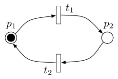
Figure 1. A simple P/T net $N$.

We need to consider another kind of weak semantics of P/T nets that is related to C/E nets in that markings hold at most one token.

[P/T restricted weak firing semantics] Let $N=(P,\,T,\,{\rm Phys.~{}Rev.~{}E}{-},\,{-^{\circ}})$ be a P/T net, $X,Y\subseteq P$ and $\mathcal{U}\in\mathcal{M}_{T}$. Write:

$$N_{X}\Rightarrow_{\mathcal{U}}N_{Y}\quad\stackrel{{\scriptstyle\mathrm{def}}}{{=}}\quad Y\cup{\rm Phys.~{}Rev.~{}E}{\mathcal{U}}=X\cup{\mathcal{U}^{\circ}}.$$

where the operation $\cup$ refers to multiset union and the sets $Y$ and $X$ are considered as multisets.

Note that Definition 1 is a special case of Definition 1, when considering just 1-safe markings.

3. C/E Nets with boundaries

In Definition 2.1 we recalled the notion of C/E nets together with a firing semantics in Definition 2.1.

In this section we introduce a way of extending C/E nets with boundaries that allows nets to be composed along a common boundary. We give a labelled semantics to C/E nets with boundaries in Section 3.1. The resulting model is semantically equivalent to the strong semantics of the Petri Calculus, introduced in Section 6; the translations are amongst the translations described in Sections 8 and 9.

In order to illustrate marked C/E nets with boundaries, it will first be useful to change the traditional graphical representation of a net and use a representation closer in spirit to that traditionally used in string diagrams. The diagram on the left in Fig. 2 demonstrates the traditional graphical representation of a (marked) net. Places are circles; a marking is represented by the presence or absence of tokens. Each transition $t\in T$ is a rectangle; there are directed edges from each place in ${\rm Phys.~{}Rev.~{}E}{t}$ to $t$ and from $t$ to each place in ${t^{\circ}}$. This graphical language is a particular way of drawing hypergraphs; the right diagram in Fig. 2 demonstrates another graphical representation, more suitable for drawing nets with boundaries. Places are again circles, but each place has exactly two ports (usually drawn as small black triangles): one in-port, which we shall usually draw on the left, and one out-port, usually drawn on the right. Transitions are simply undirected links—each link can connect to any number of ports. Connecting $t$ to the out-port of $p$ means that $p\in{\rm Phys.~{}Rev.~{}E}{t}$, connecting $t$ to $p$’s in-port means that $p\in{t^{\circ}}$. The position of the “bar” in the graphical representation of each link is irrelevant, they are used solely to distinguish individual links. A moment’s thought ought to convince the reader that the two ways of drawing nets are equivalent, in that they both faithfully represent the same underlying formal structures.

      

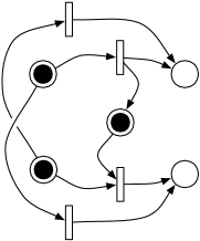
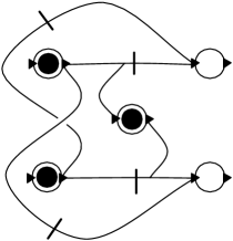
Figure 2. Traditional and alternative graphical representations of a net.

Independence of transitions in C/E nets is an important concept—only independent transitions are permitted to fire concurrently. We will say that any two transitions $t$, $u$ with $t\neq u$ that are not independent are in contention, and write $t\#u$. Then, in ordinary C/E nets, $t\#u$ precisely when $t\neq u$ and ${\rm Phys.~{}Rev.~{}E}{t}\cap{\rm Phys.~{}Rev.~{}E}{u}\neq\varnothing$ or ${t^{\circ}}\cap{u^{\circ}}\neq\varnothing$. In particular, the firing rule for the semantics of C/E nets (Definition 2.1) can be equivalently restated as follows:

$$N_{X}\rightarrow_{U}N_{Y}\ \stackrel{{\scriptstyle\mathrm{def}}}{{=}}\ {\rm Phys.~{}Rev.~{}E}{U}\subseteq X,\,{U^{\circ}}\cap X=\varnothing,\,Y=(X\backslash{\rm Phys.~{}Rev.~{}E}{U})\cup{U^{\circ}}\ \&\ \forall u,v\in U.\,\neg(u\#v).$$

Our models connect transitions to ports on boundaries. Nets that share a common boundary can be composed—the transitions of the composed net are certain synchronisations between the transitions of the underlying nets, as we will explain below. Connecting two C/E net transitions to the same port on the boundary introduces a new source of contention—moreover this information must be preserved by composition. For this reason the contention relation is an explicit part of the structure of C/E nets with boundaries.

The model of C/E nets with boundaries originally proposed in [49] lacked the contention relation and therefore the translation between Petri calculus terms and nets was more involved. Moreover, the model of C/E nets with boundaries therein was less well-behaved in that composition was suspect; for example bisimilarity was not a congruence with respect to it. Incorporating the contention relation as part of the structure allows us to repair these shortcomings and obtain a simple translation of the Petri calculus that is similar to the other translations in this paper.

We start by introducing a version of C/E nets with boundaries. Let $\underline{k},\,\underline{l},\underline{m},\,\underline{n}$ range over finite ordinals.

[C/E nets with boundaries] Let $m,n\in\mathbb{N}$. A (finite, marked) C/E net with boundaries $N_{X}\colon m\to n$, is an 8-tuple $(P,\,T,X,\,\#,\,{\rm Phys.~{}Rev.~{}E}{-},\,{-^{\circ}},\,{{}^{\bullet}{-}},\,{{-}^{\bullet}})$ where: $-$

$(P,\,T,\,{\rm Phys.~{}Rev.~{}E}{-},\,{-^{\circ}})$ is a finite C/E net;

${{}^{\bullet}{-}}\colon T\to 2^{\underline{m}}$ and ${{-}^{\bullet}}\colon T\to 2^{\underline{n}}$ connect each transition to a set of ports on the left boundary $\underline{m}$ and right boundary $\underline{n}$;

$X\subseteq P$ is the marking;

$\#$ is a symmetric and irreflexive binary relation on $T$ called contention. The contention relation must include all those transitions that are not independent in the underlying C/E net, and those that share a place on the boundary, i.e. for all $t,u\in T$ where $t\neq u$:

1. if ${\rm Phys.~{}Rev.~{}E}{t}\mathrel{\cap}{\rm Phys.~{}Rev.~{}E}{u}\neq\varnothing$, then $t\#u$;

2. if ${t^{\circ}}\mathrel{\cap}{u^{\circ}}\neq\varnothing$, then $t\#u$;

3. if ${{}^{\bullet}{t}}\cap{{}^{\bullet}{u}}\neq\varnothing$, then $t\#u$;

4. if ${{t}^{\bullet}}\cap{{u}^{\bullet}}\neq\varnothing$, then $t\#u$.

Transitions $t,t^{\prime}\in T$ are said to have the same footprint when ${\rm Phys.~{}Rev.~{}E}{t}={\rm Phys.~{}Rev.~{}E}{t^{\prime}}$, ${t^{\circ}}={t^{\prime\circ}}$, ${{}^{\bullet}{t}}={{}^{\bullet}{t^{\prime}}}$ and ${{t}^{\bullet}}={{t^{\prime}}^{\bullet}}$. From an operational point of view, transitions with the same footprint are indistinguishable. We assume that if $t$ and $t^{\prime}$ have the same footprint then $t=t^{\prime}$. This assumption is operationally harmless and somewhat simplifies reasoning about composition.

An example of C/E net with boundaries is pictured in Fig. 3. Note that $\zeta$ is a transition with empty pre and postset, and transitions $\delta$ and $\gamma$ are in contention because they share a port.

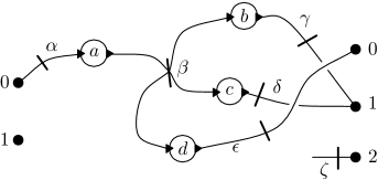
Figure 3. Representation of a net with boundaries $N_{\varnothing}:2\to 3$. Here $T=\{\alpha,\,\beta,\,\gamma,\,\delta,\,\epsilon,\,\zeta\}$ and $P=\{a,\,b,\,c,\,d\}$. The non-empty values of ${\rm Phys.~{}Rev.~{}E}{-}$ and ${-^{\circ}}$ are: ${\alpha^{\circ}}=\{a\}$, ${\rm Phys.~{}Rev.~{}E}{\beta}=\{a\}$, ${\beta^{\circ}}=\{b,c,d\}$, ${\rm Phys.~{}Rev.~{}E}{\gamma}=\{b\}$, ${\rm Phys.~{}Rev.~{}E}{\delta}=\{c\}$, ${\rm Phys.~{}Rev.~{}E}{\epsilon}=\{d\}$. The non-empty values of ${{}^{\bullet}{-}}$ and ${{-}^{\bullet}}$ are: ${{}^{\bullet}{\alpha}}=\{0\}$, ${{\epsilon}^{\bullet}}=\{0\}$, ${{\gamma}^{\bullet}}=\{1\}$, ${{\delta}^{\bullet}}=\{1\}$, ${{\zeta}^{\bullet}}=\{2\}$. Of course when the same port name appears in the left and right boundaries (e.g., $0$) it denotes different nodes.

The notion of independence of transitions extends to C/E nets with boundaries: $t,u\in T$ are said to be independent when $\neg(t\#u)$. We say that a set $U$ of transitions is mutually independent if $\forall u,v\in U.\;\neg(u\#v)$.

The obvious notion of homomorphism between two C/E nets extends that of ordinary nets: given nets $N_{X},M_{Y}\colon m\to n$, $f\colon N_{X}\to M_{Y}$ is a pair of functions $f_{T}\colon T_{N}\to T_{M}$, $f_{P}\colon P_{N}\to P_{M}$ such that $f_{P}(X)=Y$, $f_{T}(t)\#f_{T}(u)$ implies $t\#u$, ${\rm Phys.~{}Rev.~{}E}{-}_{N}\mathrel{;}2^{f_{P}}=f_{T}\mathrel{;}{\rm Phys.~{}Rev.~{}E}{-}_{M}$, ${-^{\circ}}_{N}\mathrel{;}2^{f_{P}}=f_{T}\mathrel{;}{-^{\circ}}_{M}$, ${{}^{\bullet}{-}}_{N}=f_{T}\mathrel{;}{{}^{\bullet}{-}}_{M}$ and ${{-}^{\bullet}}_{N}=f_{T}\mathrel{;}{{-}^{\bullet}}_{M}$. A homomorphism is an isomorphism iff its two components are bijections; we write $N_{X}\cong M_{Y}$ when there is an isomorphism from $N_{X}$ to $M_{Y}$.

The main operation on nets with boundaries is composition along a common boundary. That is, given nets $M_{X}\colon l\to m$, $N_{Y}\colon m\to n$ we will define a net $M_{X};N_{Y}\colon l\to n$. Roughly, the transitions of the composed net $M_{X};N_{Y}$ are certain sets of transitions of the two underlying nets that synchronise on the common boundary. Thus in order to define the composition of nets along a shared boundary, we must first introduce the concept of synchronisation.

[Synchronisation of C/E nets] Let $M_{X}\colon l\to m$ and $N_{Y}\colon m\to n$ be C/E nets. A synchronisation is a pair $(U,V)$, with $U\subseteq T_{M}$ and $V\subseteq T_{N}$ mutually independent sets of transitions such that: $-$

$U+V\neq\varnothing$;

${{U}^{\bullet}}={{}^{\bullet}{V}}$. The set of synchronisations inherits an ordering pointwise from the subset order, i.e.  we let $(U^{\prime},\,V^{\prime})\subseteq(U,\,V)$ when $U^{\prime}\subseteq U$ and $V^{\prime}\subseteq V$. A synchronisation is said to be minimal when it is minimal with respect to this order. Let $Synch(M,N)$ denote the set of minimal synchronisations. Note that synchronisations do not depend on the markings of the underlying nets, but on the sets of transitions $T_{M}$ and $T_{N}$. Consequently, $Synch(M,N)$ is finite because $T_{M}$ and $T_{N}$ are so. It could be also the case that $Synch(M,N)$ is the empty set . Notice that any transition in $M$ or $N$ not connected to the shared boundary $m$ (trivially) induces a minimal synchronisation—for instance if $t\in T_{M}$ with ${{t}^{\bullet}}=\varnothing$, then $(\{t\},\,\varnothing)$ is a minimal synchronisation.

The following result shows that any synchronisation can be decomposed into a set of minimal synchronisations.

Lemma 2.

Suppose that $M_{X}:k\to n$ and $N_{Y}:n\to m$ are C/E nets with boundaries and $(U,V)$ is a synchronisation. Then there exists a finite set of minimal synchronisations $\{(U_{i},V_{i})\}_{i\in I}$ such that (i) $U_{i}\cap U_{j}=V_{i}\cap V_{j}=\varnothing$ whenever $i\neq j$, (ii) $\bigcup_{i}U_{i}=U$ and (iii) $\bigcup_{i}V_{i}=V$.

Proof 3.1.

See Appendix A.

Minimal synchronisations serve as the transitions of the composition of two nets along a common boundary. Thus, given $(U,\,V)\in Synch(M,N)$ let ${\rm Phys.~{}Rev.~{}E}{(U,\,V)}\stackrel{{\scriptstyle\mathrm{def}}}{{=}}{\rm Phys.~{}Rev.~{}E}{U}+{\rm Phys.~{}Rev.~{}E}{V}$, ${(U,\,V)^{\circ}}\stackrel{{\scriptstyle\mathrm{def}}}{{=}}{U^{\circ}}+{V^{\circ}}$, ${{}^{\bullet}{(U,\,V)}}\stackrel{{\scriptstyle\mathrm{def}}}{{=}}{{}^{\bullet}{U}}$ and ${{(U,\,V)}^{\bullet}}\stackrel{{\scriptstyle\mathrm{def}}}{{=}}{{V}^{\bullet}}$. For $(U,\,V)$, $(U^{\prime},\,V^{\prime})\in Synch(M,N)$, $(U,V)\#(U^{\prime},V^{\prime})$ iff $(U,V)\neq(U^{\prime},V^{\prime})$ and $-$

$U\cap U^{\prime}\neq\varnothing$ or $\exists u\in U,u^{\prime}\in U^{\prime}$ such that $u\#u^{\prime}$ (as transitions of $M$), or

$V\cap V^{\prime}\neq\varnothing$ $\exists v\in V,v^{\prime}\in V^{\prime}$ such that $v\#v^{\prime}$ (as transitions of $N$);

Having introduced minimal synchronisations we may now define the composition of two C/E nets that share a common boundary.

[Composition of C/E nets with boundaries] When $M_{X}\colon l\to m$ and $N_{Y}\colon m\to n$ are C/E nets, define their composition, $M;N_{X+Y}\colon l\to n$, as follows: $-$

places are $P_{M}+P_{N}$, the “enforced” disjoint union of places of $M$ and $N$;

transitions are obtained from the set of minimal synchronisations $Synch(M,N)$, after removing any redundant transitions with equal footprint;

the marking is $X+Y$. We must verify that $\#$ as defined on $Synch(M,N)$ above satisfies the conditions on the contention relation given in Definition 2. Indeed if ${\rm Phys.~{}Rev.~{}E}{(U,V)}\cap{\rm Phys.~{}Rev.~{}E}{(U^{\prime},V^{\prime})}\neq\varnothing$ then one of ${\rm Phys.~{}Rev.~{}E}{U}\cap{\rm Phys.~{}Rev.~{}E}{U^{\prime}}$ and ${\rm Phys.~{}Rev.~{}E}{V}\cap{\rm Phys.~{}Rev.~{}E}{V^{\prime}}$ must be non-empty. Without loss of generality, if the first is nonempty then there exist $u\in U$, $u^{\prime}\in U^{\prime}$ with ${\rm Phys.~{}Rev.~{}E}{u}\cap{\rm Phys.~{}Rev.~{}E}{u^{\prime}}\neq\varnothing$, thus either $u=u^{\prime}$, in which case $U\cap U^{\prime}\neq\varnothing$, or $u\#u^{\prime}$ in $M$—thus by construction ${\rm Phys.~{}Rev.~{}E}{(U,V)}\#{\rm Phys.~{}Rev.~{}E}{(U^{\prime},V^{\prime})}$ in the composition, as required. The remaining conditions are similarly easily shown to hold.

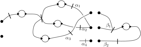
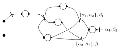
Figure 4. Composition of two C/E nets.

An example of a composition of two C/E nets is illustrated in Fig. 4.

Remark 3.

Two transitions in the composition of two C/E nets may be in contention even though they are mutually independent in the underlying C/E net, as illustrated by Fig. 5. $\Box$

Figure 5. Composition of two nets with boundaries. Note that $\alpha_{1}\#\alpha_{2}$ implicitly in the leftmost net, and $(\alpha_{1},\beta)\#(\alpha_{2},\beta)$ in the composition. This is emphasised graphically with the jagged line in the rightmost diagram.

Remark 4.

Any ordinary C/E net $N$ (Definition 2.1) can be considered as a net with boundaries $N:0\to 0$ as there is exactly one choice for functions ${{}^{\bullet}{-}},{{-}^{\bullet}}:T\to 2^{\underline{0}}$ and the contention relation consists of all pairs of transitions that are not independent in $N$. Composition of two nets $N:0\to 0$ and $M:0\to 0$ is then just the disjoint union of the two nets: the set of places is $P_{N}+P_{M}$, the minimal synchronisations are precisely $(\{t\},\varnothing)$, $t\in T_{N}$ and $(\varnothing,\{t^{\prime}\})$, $t^{\prime}\in T_{M}$, and the contention relation is the union of the contention relations of $N$ and $M$. $\Box$

3.1. Labelled semantics of C/E nets with boundaries

Figure 6. Part of a labelled transition system for simple C/E net $2\to 3$. The symbol $*$ is used as shorthand for any label in $\{0,1\}$.

For any $k\in\mathbb{N}$, there is a bijection ${\ulcorner-\urcorner}:2^{\underline{k}}\to\{0,1\}^{k}$ with

$${\ulcorner U\urcorner}_{i}\stackrel{{\scriptstyle\mathrm{def}}}{{=}}\begin{cases}1&\text{if }i\in U\\ 0&\text{otherwise.}\end{cases}$$

Similarly, with slight abuse of notation, we define ${\ulcorner-\urcorner}:\mathcal{M}_{\underline{k}}\to\mathbb{N}^{k}$ by

$${\ulcorner\mathcal{U}\urcorner}_{i}\stackrel{{\scriptstyle\mathrm{def}}}{{=}}\mathcal{U}(i)$$

[C/E Net Labelled Semantics] Let $N:m\to n$ be a C/E net with boundaries and $X,Y\subseteq P_{N}$. Write:

$$N_{X}\raise 1.0pt\hbox{$\;\mathrel{\mathop{\mathchoice{\leavevmode\vtop{\halign{\hfil$\displaystyle#$\hfil\cr\scriptstyle\xrightarrow{\,\alpha\,}\cr{\lower 1.99997pt\hbox{$\scriptstyle{}_{\beta}$}}\crcr}}}{\leavevmode\vtop{\halign{\hfil$\textstyle#$\hfil\cr\scriptstyle\xrightarrow{\,\alpha\,}\cr{\lower 1.99997pt\hbox{$\scriptstyle{}_{\beta}$}}\crcr}}}{\leavevmode\vtop{\halign{\hfil$\scriptstyle#$\hfil\cr\scriptstyle\xrightarrow{\,\alpha\,}\cr{\lower 1.39998pt\hbox{$\scriptstyle{}_{\beta}$}}\crcr}}}{\leavevmode\vtop{\halign{\hfil$\scriptscriptstyle#$\hfil\cr\scriptstyle\xrightarrow{\,\alpha\,}\cr{\lower 0.99998pt\hbox{$\scriptstyle{}_{\beta}$}}\crcr}}}}}\;$}N_{Y}\quad\stackrel{{\scriptstyle\mathrm{def}}}{{=}}\quad\exists\text{ mutually independent }U\subseteq T_{N}\text{ s.t. }\\ N_{X}\rightarrow_{U}N_{Y},\ \alpha={\ulcorner{{}^{\bullet}{U}}\urcorner}\ \&\ \beta={\ulcorner{{U}^{\bullet}}\urcorner}$$ (1)

It is worth emphasising that no information about precisely which set $U$ of transitions has been fired is carried by transition labels, merely the effect of the firing on the boundaries. Notice that we always have $N_{X}\raise 1.0pt\hbox{$\;\mathrel{\mathop{\mathchoice{\leavevmode\vtop{\halign{\hfil$\displaystyle#$\hfil\cr\scriptstyle\xrightarrow{\,0^{m}\,}\cr{\lower 1.99997pt\hbox{$\scriptstyle{}_{0^{n}}$}}\crcr}}}{\leavevmode\vtop{\halign{\hfil$\textstyle#$\hfil\cr\scriptstyle\xrightarrow{\,0^{m}\,}\cr{\lower 1.99997pt\hbox{$\scriptstyle{}_{0^{n}}$}}\crcr}}}{\leavevmode\vtop{\halign{\hfil$\scriptstyle#$\hfil\cr\scriptstyle\xrightarrow{\,0^{m}\,}\cr{\lower 1.39998pt\hbox{$\scriptstyle{}_{0^{n}}$}}\crcr}}}{\leavevmode\vtop{\halign{\hfil$\scriptscriptstyle#$\hfil\cr\scriptstyle\xrightarrow{\,0^{m}\,}\cr{\lower 0.99998pt\hbox{$\scriptstyle{}_{0^{n}}$}}\crcr}}}}}\;$}N_{X}$, as the empty set of transitions is vacuously mutually independent.

A transition $N_{X}\raise 1.0pt\hbox{$\;\mathrel{\mathop{\mathchoice{\leavevmode\vtop{\halign{\hfil$\displaystyle#$\hfil\cr\scriptstyle\xrightarrow{\,\alpha\,}\cr{\lower 1.99997pt\hbox{$\scriptstyle{}_{\beta}$}}\crcr}}}{\leavevmode\vtop{\halign{\hfil$\textstyle#$\hfil\cr\scriptstyle\xrightarrow{\,\alpha\,}\cr{\lower 1.99997pt\hbox{$\scriptstyle{}_{\beta}$}}\crcr}}}{\leavevmode\vtop{\halign{\hfil$\scriptstyle#$\hfil\cr\scriptstyle\xrightarrow{\,\alpha\,}\cr{\lower 1.39998pt\hbox{$\scriptstyle{}_{\beta}$}}\crcr}}}{\leavevmode\vtop{\halign{\hfil$\scriptscriptstyle#$\hfil\cr\scriptstyle\xrightarrow{\,\alpha\,}\cr{\lower 0.99998pt\hbox{$\scriptstyle{}_{\beta}$}}\crcr}}}}}\;$}N_{Y}$ indicates that the C/E net $N$ evolves from marking $X$ to marking $Y$ by firing a set of transitions whose connections are recorded by $\alpha$ on the left interface and $\beta$ on the right interface. We give an example in Fig. 6.

Labelled semantics is compatible with composition in the following sense.

Theorem 5.

Suppose that $M:k\to n$ and $N:n\to m$ are C/E nets with boundaries, and $X,X^{\prime}\subseteq P_{M}$ and $Y,Y^{\prime}\subseteq P_{N}$ markings. Then $M;N_{X+Y}\raise 1.0pt\hbox{$\;\mathrel{\mathop{\mathchoice{\leavevmode\vtop{\halign{\hfil$\displaystyle#$\hfil\cr\scriptstyle\xrightarrow{\,\alpha\,}\cr{\lower 1.99997pt\hbox{$\scriptstyle{}_{\beta}$}}\crcr}}}{\leavevmode\vtop{\halign{\hfil$\textstyle#$\hfil\cr\scriptstyle\xrightarrow{\,\alpha\,}\cr{\lower 1.99997pt\hbox{$\scriptstyle{}_{\beta}$}}\crcr}}}{\leavevmode\vtop{\halign{\hfil$\scriptstyle#$\hfil\cr\scriptstyle\xrightarrow{\,\alpha\,}\cr{\lower 1.39998pt\hbox{$\scriptstyle{}_{\beta}$}}\crcr}}}{\leavevmode\vtop{\halign{\hfil$\scriptscriptstyle#$\hfil\cr\scriptstyle\xrightarrow{\,\alpha\,}\cr{\lower 0.99998pt\hbox{$\scriptstyle{}_{\beta}$}}\crcr}}}}}\;$}M;N_{X^{\prime}+Y^{\prime}}$ iff there exists $\gamma\in\{0,1\}^{n}$ such that

$$M_{X}\raise 1.0pt\hbox{$\;\mathrel{\mathop{\mathchoice{\leavevmode\vtop{\halign{\hfil$\displaystyle#$\hfil\cr\scriptstyle\xrightarrow{\,\alpha\,}\cr{\lower 1.99997pt\hbox{$\scriptstyle{}_{\gamma}$}}\crcr}}}{\leavevmode\vtop{\halign{\hfil$\textstyle#$\hfil\cr\scriptstyle\xrightarrow{\,\alpha\,}\cr{\lower 1.99997pt\hbox{$\scriptstyle{}_{\gamma}$}}\crcr}}}{\leavevmode\vtop{\halign{\hfil$\scriptstyle#$\hfil\cr\scriptstyle\xrightarrow{\,\alpha\,}\cr{\lower 1.39998pt\hbox{$\scriptstyle{}_{\gamma}$}}\crcr}}}{\leavevmode\vtop{\halign{\hfil$\scriptscriptstyle#$\hfil\cr\scriptstyle\xrightarrow{\,\alpha\,}\cr{\lower 0.99998pt\hbox{$\scriptstyle{}_{\gamma}$}}\crcr}}}}}\;$}M_{X^{\prime}}\text{ and }N_{Y}\raise 1.0pt\hbox{$\;\mathrel{\mathop{\mathchoice{\leavevmode\vtop{\halign{\hfil$\displaystyle#$\hfil\cr\scriptstyle\xrightarrow{\,\gamma\,}\cr{\lower 1.99997pt\hbox{$\scriptstyle{}_{\beta}$}}\crcr}}}{\leavevmode\vtop{\halign{\hfil$\textstyle#$\hfil\cr\scriptstyle\xrightarrow{\,\gamma\,}\cr{\lower 1.99997pt\hbox{$\scriptstyle{}_{\beta}$}}\crcr}}}{\leavevmode\vtop{\halign{\hfil$\scriptstyle#$\hfil\cr\scriptstyle\xrightarrow{\,\gamma\,}\cr{\lower 1.39998pt\hbox{$\scriptstyle{}_{\beta}$}}\crcr}}}{\leavevmode\vtop{\halign{\hfil$\scriptscriptstyle#$\hfil\cr\scriptstyle\xrightarrow{\,\gamma\,}\cr{\lower 0.99998pt\hbox{$\scriptstyle{}_{\beta}$}}\crcr}}}}}\;$}N_{Y^{\prime}}.$$

Proof 3.2.

See Appendix A.

The above result is enough to show that bisimilarity is a congruence with respect to the composition of nets over a common boundary.

Proposition 6.

Bisimilarity of C/E nets is a congruence w.r.t. ‘ $\mathrel{;}$’.

Proof 3.3.

See Appendix A.

Remark 7.

Consider the composition of the three nets with boundaries below.

The result is a net with boundaries $0\to 0$ with a single place and a single consume/produce loop transition. As we have observed in Remark 1, this transition cannot fire with the semantics of nets that we have considered so far. Globally, the transition cannot fire because its postset is included in the original marking. The fact that the transition cannot fire is also reflected locally, in light of Theorem 5: indeed, locally, for the transition to be able to fire, there would need to be a transition $N_{\{\star\}}\raise 1.0pt\hbox{$\;\mathrel{\mathop{\mathchoice{\leavevmode\vtop{\halign{\hfil$\displaystyle#$\hfil\cr\scriptstyle\xrightarrow{\,11\,}\cr{\lower 1.99997pt\hbox{$\scriptstyle{}_{11}$}}\crcr}}}{\leavevmode\vtop{\halign{\hfil$\textstyle#$\hfil\cr\scriptstyle\xrightarrow{\,11\,}\cr{\lower 1.99997pt\hbox{$\scriptstyle{}_{11}$}}\crcr}}}{\leavevmode\vtop{\halign{\hfil$\scriptstyle#$\hfil\cr\scriptstyle\xrightarrow{\,11\,}\cr{\lower 1.39998pt\hbox{$\scriptstyle{}_{11}$}}\crcr}}}{\leavevmode\vtop{\halign{\hfil$\scriptscriptstyle#$\hfil\cr\scriptstyle\xrightarrow{\,11\,}\cr{\lower 0.99998pt\hbox{$\scriptstyle{}_{11}$}}\crcr}}}}}\;$}N_{\{\star\}}$, but this is not possible because there is a token present in the postset of the transition connected to the lower left boundary. It is possible to relax the semantics of nets in order to allow such transitions to fire, as we will explain in Remark 17. $\Box$

Remark 8.

In Remark 4 we noted that any ordinary net $N$ can be considered as a net with boundaries $N:0\to 0$. For such nets, the transition system of Definition 6 has transitions with only one label (since there is nothing to observe on the boundaries) and thus corresponds to an unlabelled step-firing semantics transition system. In particular, it follows that, while the transition systems generated for nets $N:0\to 0$ are different, they are all bisimilar; we feel that this is compatible with the usual view on labelled equivalences in that they capture behaviour that is observable from the outside: a net $N:0\to 0$ does not have a boundary and thus there is no way of interacting with it and therefore no way of telling apart two such nets. One can, of course, allow the possibility of observing the firing of certain transitions (possibly all) by connecting them to ports on the boundary. Let $N$ be a net with $n=\#T_{N}$ transitions. A corresponding net with boundaries that makes transitions observable over the right interface is as follows: $N\colon 0\to n$ with ${}^{\bullet}t=\varnothing$ for all $t\in T_{N}$, $\_^{\bullet}\colon T_{N}\to\underline{n}$ any injective function, and the contention relation containing only those pairs of transitions that are in contention in the underlying C/E net $N$. $\Box$

4. P/T nets with boundaries

This section extends the notion of nets with boundaries to P/T nets. The contention relation no longer plays a role, and connections of transitions to boundary ports are weighted.

[P/T net with boundaries] Let $m,n\in\mathbb{N}$. A (finite, marked) P/T net with boundaries $N_{\mathcal{X}}:m\rightarrow n$ is a tuple $N=(P,T,{\rm Phys.~{}Rev.~{}E}{-},{-^{\circ}},{}^{\bullet}-,-^{\bullet})$ where: $-$

$(P,T,{\rm Phys.~{}Rev.~{}E}{-},{-^{\circ}})$ is a finite P/T net;

${}^{\bullet}-:T\rightarrow\mathcal{M}_{\underline{m}}$ and $-^{\bullet}:T\rightarrow\mathcal{M}_{\underline{n}}$ are functions that assign transitions to the left and right boundaries of $N$;

$\mathcal{X}\in\mathcal{M}_{P}$. As in Definition 2 we assume that transitions have distinct footprints.

Remark 9.

For reasons that will become clear when we study the process algebraic account, we will sometimes refer to P/T nets with boundaries that have markings which are subsets ($X\subseteq P$) of places instead of a multiset ($\mathcal{X}\in\mathcal{M}_{P}$) of places as weak C/E nets with boundaries. $\Box$

The notion of net homomorphism extends to marked P/T nets with the same boundaries: given $N_{\mathcal{X}},M_{\mathcal{Y}}:m\rightarrow n$, $f:N_{\mathcal{X}}\rightarrow M_{\mathcal{Y}}$ is a pair of functions $f_{T}\colon T_{N}\to T_{M}$, $f_{P}\colon P_{N}\to P_{M}$ such that $f_{P}(\mathcal{X})=\mathcal{Y}$, ${\rm Phys.~{}Rev.~{}E}{-}_{N}\mathrel{;}2^{f_{P}}=f_{T}\mathrel{;}{\rm Phys.~{}Rev.~{}E}{-}_{M}$, ${-^{\circ}}_{N}\mathrel{;}2^{f_{P}}=f_{T}\mathrel{;}{-^{\circ}}_{M}$, ${{}^{\bullet}{-}}_{N}=f_{T}\mathrel{;}{{}^{\bullet}{-}}_{M}$ and ${{-}^{\bullet}}_{N}=f_{T}\mathrel{;}{{-}^{\bullet}}_{M}$. A homomorphism is an isomorphism if its two components are bijections. We write $N_{\mathcal{X}}\cong M_{\mathcal{Y}}$ if there is an isomorphism from $N_{\mathcal{X}}$ to $M_{\mathcal{Y}}$.

In order to compose P/T nets with boundaries we need to consider a more general notion of synchronisation. This is because synchronisations of P/T involve multisets of transitions and there is no requirement of mutual independence. The definitions of ${{}^{\bullet}{-}}$ and ${{-}^{\bullet}}$ extend for multisets in the obvious way by letting ${{}^{\bullet}{\mathcal{U}}}\stackrel{{\scriptstyle\mathrm{def}}}{{=}}\bigcup_{t\in T}\mathcal{U}(t)\cdot{{}^{\bullet}{t}}$ and ${{\mathcal{U}}^{\bullet}}\stackrel{{\scriptstyle\mathrm{def}}}{{=}}\bigcup_{t\in T}\mathcal{U}(t)\cdot{{t}^{\bullet}}$.

[Synchronisation of P/T nets] A synchronization between nets $M_{\mathcal{X}}:l\rightarrow m$ and $N_{\mathcal{Y}}:m\rightarrow n$ is a pair $({\mathcal{U}},{\mathcal{V}})$, with ${\mathcal{U}}\in\mathcal{M}_{T_{M}}$ and ${\mathcal{V}}\in\mathcal{M}_{T_{N}}$ multisets of transitions such that: $-$

${\mathcal{U}}+{\mathcal{V}}\neq\varnothing$;

${{{\mathcal{U}}}^{\bullet}}={{}^{\bullet}{{\mathcal{V}}}}$. The set of synchronisations inherits an ordering from the subset relation, i.e. $({\mathcal{U}}^{\prime},\,{\mathcal{V}}^{\prime})\subseteq({\mathcal{U}},\,{\mathcal{V}})$ when ${\mathcal{U}}^{\prime}\subseteq{\mathcal{U}}$ and ${\mathcal{V}}^{\prime}\subseteq{\mathcal{V}}$. A synchronisation is said to be minimal when it is minimal with respect to this order.

Let $Synch(M,N)$ denote the set of minimal synchronisations, an unordered set. This set is always finite—this is an easy consequence of Dickson’s Lemma [23, Lemma A].

Lemma 10.

The set of minimal synchronisations $Synch(M,N)$ is finite.

The following result is comparable to Lemma 2 in the P/T net setting—any synchronisation can be written as a linear combination of minimal synchronisations.

Lemma 11.

Suppose that $M_{\mathcal{X}}\colon l\to m$ and $N_{\mathcal{Y}}\colon m\to n$ are P/T nets with boundaries and $(\mathcal{U},\mathcal{V})$ is a synchronisation. Then there exist a finite family $\{(b_{i},(\mathcal{U}_{i},\mathcal{V}_{i}))\}_{i\in I}$ where each $b_{i}\in\mathbb{N}_{+}$, $(\mathcal{U}_{i},\mathcal{V}_{i})\in Synch(M,N)$ where for any $i,j\in I$, $(\mathcal{U}_{i},\mathcal{V}_{i})=(\mathcal{U}_{j},\mathcal{V}_{j})$ implies that $i=j$, such that $\bigcup_{i\in I}b_{i}\cdot\mathcal{U}_{i}=\mathcal{U}$ and $\bigcup_{i\in I}b_{i}\cdot\mathcal{V}_{i}=\mathcal{V}$.

Proof 4.1.

See Appendix B.

Given $(\mathcal{U},\,\mathcal{V})\in Synch(M,N)$, let ${\rm Phys.~{}Rev.~{}E}{(\mathcal{U},\,\mathcal{V})}\stackrel{{\scriptstyle\mathrm{def}}}{{=}}{\rm Phys.~{}Rev.~{}E}{\mathcal{U}}+{\rm Phys.~{}Rev.~{}E}{\mathcal{V}}\in\mathcal{M}_{P_{M}+P_{N}}$, ${(\mathcal{U},\,\mathcal{V})^{\circ}}\stackrel{{\scriptstyle\mathrm{def}}}{{=}}{\mathcal{U}^{\circ}}+{\mathcal{V}^{\circ}}\in\mathcal{M}_{P_{M}+P_{N}}$, ${{}^{\bullet}{(\mathcal{U},\,\mathcal{V})}}\stackrel{{\scriptstyle\mathrm{def}}}{{=}}{{}^{\bullet}{\mathcal{U}}}\in\mathcal{M}_{\underline{l}}$ and ${{(\mathcal{U},\,\mathcal{V})}^{\bullet}}\stackrel{{\scriptstyle\mathrm{def}}}{{=}}{{\mathcal{V}}^{\bullet}}\in\mathcal{M}_{\underline{n}}$.

[Composition of P/T nets with boundaries] If $M_{\mathcal{X}}\colon l\to m$, $N_{\mathcal{Y}}\colon m\to n$ are P/T nets with boundaries, define their composition, $M_{\mathcal{X}};N_{\mathcal{Y}}\colon l\to n$, as follows: $-$

places are $P_{M}+P_{N}$;

transitions are obtained from set $Synch(M,N)$, after removing any redundant transitions with equal footprints (c.f.  Definition 3.1);

the marking is $\mathcal{X}+\mathcal{Y}$.

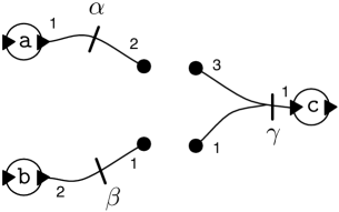
(a) Two P/T nets with boundaries $M$ (left) and $N$(right).

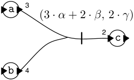
(b) Composition $M;N$.

Figure 7. Composition of P/T nets with boundaries.

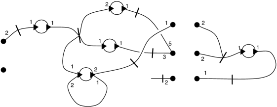
Figure 8. Composition of P/T nets with boundaries.

Figure 7(b) shows the sequential composition of the nets $M$ and $N$ depicted in Fig. 7(a). The set of minimal synchronization between $M$ and $N$ consists just in the pair $(\mathcal{U},\mathcal{V})$ with $\mathcal{U}=\{\alpha,\alpha,\alpha,\beta,\beta\}$ and $\mathcal{V}=\{\gamma,\gamma\}$. In other words, to synchronise over the shared interface $M$ should fire transition $\alpha$ three times (which consumes three tokens from $\mathtt{a}$) and $\beta$ twice (which consumes four tokens from $\mathtt{b}$) and $N$ should fire $\gamma$ twice (which produces two tokens in $\mathtt{c}$). The equivalent net describing the synchronised composition of $M$ and $N$ over their common interface is a net that contains exactly one transition, which consumes three tokens from $\mathtt{a}$, four tokens from $\mathtt{b}$ and produces two tokens in $\mathtt{c}$, as illustrated in Fig. 7(b). A more complex example of composition of P/T nets is given in Fig. 8.

4.1. Labelled semantics of P/T nets with boundaries

We give two versions of labelled semantics, one corresponding to the standard semantics and one to the banking semantics.

[Strong Labelled Semantics] Let $N:m\rightarrow n$ be a P/T net and $\mathcal{X},\mathcal{Y}\in\mathcal{M}_{P_{N}}$. We write

$$N_{\mathcal{X}}\raise 1.0pt\hbox{$\;\mathrel{\mathop{\mathchoice{\leavevmode\vtop{\halign{\hfil$\displaystyle#$\hfil\cr\scriptstyle\xrightarrow{\,\alpha\,}\cr{\lower 1.99997pt\hbox{$\scriptstyle{}_{\beta}$}}\crcr}}}{\leavevmode\vtop{\halign{\hfil$\textstyle#$\hfil\cr\scriptstyle\xrightarrow{\,\alpha\,}\cr{\lower 1.99997pt\hbox{$\scriptstyle{}_{\beta}$}}\crcr}}}{\leavevmode\vtop{\halign{\hfil$\scriptstyle#$\hfil\cr\scriptstyle\xrightarrow{\,\alpha\,}\cr{\lower 1.39998pt\hbox{$\scriptstyle{}_{\beta}$}}\crcr}}}{\leavevmode\vtop{\halign{\hfil$\scriptscriptstyle#$\hfil\cr\scriptstyle\xrightarrow{\,\alpha\,}\cr{\lower 0.99998pt\hbox{$\scriptstyle{}_{\beta}$}}\crcr}}}}}\;$}N_{\mathcal{Y}}\quad\stackrel{{\scriptstyle\mathrm{def}}}{{=}}\quad\exists{\mathcal{U}}\in\mathcal{M}_{T_{N}}\text{ s.t. }N_{\mathcal{X}}\rightarrow_{\mathcal{U}}N_{\mathcal{Y}},\ \alpha={\ulcorner{{}^{\bullet}{\mathcal{U}}}\urcorner}\ \&\ \beta={\ulcorner{{\mathcal{U}}^{\bullet}}\urcorner}.$$ (2)

[Weak Labelled Semantics] Let $N:m\rightarrow n$ be a P/T net and $\mathcal{X},\mathcal{Y}\in\mathcal{M}_{P_{N}}$. We write

$$N_{\mathcal{X}}\raise 1.0pt\hbox{$\;\mathrel{\mathop{\mathchoice{\leavevmode\vtop{\halign{\hfil$\displaystyle#$\hfil\cr\scriptstyle\Longrightarrow\cr{\lower-6.00006pt\hbox{$\scriptstyle{}_{\alpha}$}}\cr{\lower 3.00003pt\hbox{$\scriptstyle{}_{\beta}$}}\crcr}}}{\leavevmode\vtop{\halign{\hfil$\textstyle#$\hfil\cr\scriptstyle\Longrightarrow\cr{\lower-6.00006pt\hbox{$\scriptstyle{}_{\alpha}$}}\cr{\lower 3.00003pt\hbox{$\scriptstyle{}_{\beta}$}}\crcr}}}{\leavevmode\vtop{\halign{\hfil$\scriptstyle#$\hfil\cr\scriptstyle\Longrightarrow\cr{\lower-4.20004pt\hbox{$\scriptstyle{}_{\alpha}$}}\cr{\lower 2.10002pt\hbox{$\scriptstyle{}_{\beta}$}}\crcr}}}{\leavevmode\vtop{\halign{\hfil$\scriptscriptstyle#$\hfil\cr\scriptstyle\Longrightarrow\cr{\lower-3.00003pt\hbox{$\scriptstyle{}_{\alpha}$}}\cr{\lower 1.50002pt\hbox{$\scriptstyle{}_{\beta}$}}\crcr}}}}}\;$}N_{\mathcal{Y}}\quad\stackrel{{\scriptstyle\mathrm{def}}}{{=}}\quad\exists{\mathcal{U}}\in\mathcal{M}_{T_{N}}\text{ s.t. }N_{\mathcal{X}}\Rightarrow_{\mathcal{U}}N_{\mathcal{Y}},\ \alpha={\ulcorner{{}^{\bullet}{\mathcal{U}}}\urcorner}\ \&\ \beta={\ulcorner{{\mathcal{U}}^{\bullet}}\urcorner}.$$ (3)

Theorem 12.

Suppose that $M\colon k\to n$ and $N\colon n\to m$ are P/T nets with boundaries, and $\mathcal{X},\mathcal{X}^{\prime}\in\mathcal{M}_{P_{M}}$ and $\mathcal{Y},\mathcal{Y}^{\prime}\in\mathcal{M}_{P_{N}}$ markings. Then

1. $M;N_{\mathcal{X}+\mathcal{Y}}\raise 1.0pt\hbox{$\;\mathrel{\mathop{\mathchoice{\leavevmode\vtop{\halign{\hfil$\displaystyle#$\hfil\cr\scriptstyle\xrightarrow{\,\alpha\,}\cr{\lower 1.99997pt\hbox{$\scriptstyle{}_{\beta}$}}\crcr}}}{\leavevmode\vtop{\halign{\hfil$\textstyle#$\hfil\cr\scriptstyle\xrightarrow{\,\alpha\,}\cr{\lower 1.99997pt\hbox{$\scriptstyle{}_{\beta}$}}\crcr}}}{\leavevmode\vtop{\halign{\hfil$\scriptstyle#$\hfil\cr\scriptstyle\xrightarrow{\,\alpha\,}\cr{\lower 1.39998pt\hbox{$\scriptstyle{}_{\beta}$}}\crcr}}}{\leavevmode\vtop{\halign{\hfil$\scriptscriptstyle#$\hfil\cr\scriptstyle\xrightarrow{\,\alpha\,}\cr{\lower 0.99998pt\hbox{$\scriptstyle{}_{\beta}$}}\crcr}}}}}\;$}M;N_{\mathcal{X}^{\prime}+\mathcal{Y}^{\prime}}$ iff there exists $\gamma\in\mathbb{N}^{n}$ such that

   $$M_{\mathcal{X}}\raise 1.0pt\hbox{$\;\mathrel{\mathop{\mathchoice{\leavevmode\vtop{\halign{\hfil$\displaystyle#$\hfil\cr\scriptstyle\xrightarrow{\,\alpha\,}\cr{\lower 1.99997pt\hbox{$\scriptstyle{}_{\gamma}$}}\crcr}}}{\leavevmode\vtop{\halign{\hfil$\textstyle#$\hfil\cr\scriptstyle\xrightarrow{\,\alpha\,}\cr{\lower 1.99997pt\hbox{$\scriptstyle{}_{\gamma}$}}\crcr}}}{\leavevmode\vtop{\halign{\hfil$\scriptstyle#$\hfil\cr\scriptstyle\xrightarrow{\,\alpha\,}\cr{\lower 1.39998pt\hbox{$\scriptstyle{}_{\gamma}$}}\crcr}}}{\leavevmode\vtop{\halign{\hfil$\scriptscriptstyle#$\hfil\cr\scriptstyle\xrightarrow{\,\alpha\,}\cr{\lower 0.99998pt\hbox{$\scriptstyle{}_{\gamma}$}}\crcr}}}}}\;$}M_{\mathcal{X}^{\prime}}\text{ and }N_{\mathcal{Y}}\raise 1.0pt\hbox{$\;\mathrel{\mathop{\mathchoice{\leavevmode\vtop{\halign{\hfil$\displaystyle#$\hfil\cr\scriptstyle\xrightarrow{\,\gamma\,}\cr{\lower 1.99997pt\hbox{$\scriptstyle{}_{\beta}$}}\crcr}}}{\leavevmode\vtop{\halign{\hfil$\textstyle#$\hfil\cr\scriptstyle\xrightarrow{\,\gamma\,}\cr{\lower 1.99997pt\hbox{$\scriptstyle{}_{\beta}$}}\crcr}}}{\leavevmode\vtop{\halign{\hfil$\scriptstyle#$\hfil\cr\scriptstyle\xrightarrow{\,\gamma\,}\cr{\lower 1.39998pt\hbox{$\scriptstyle{}_{\beta}$}}\crcr}}}{\leavevmode\vtop{\halign{\hfil$\scriptscriptstyle#$\hfil\cr\scriptstyle\xrightarrow{\,\gamma\,}\cr{\lower 0.99998pt\hbox{$\scriptstyle{}_{\beta}$}}\crcr}}}}}\;$}N_{\mathcal{Y}^{\prime}}.$$

2. $M;N_{\mathcal{X}+\mathcal{Y}}\raise 1.0pt\hbox{$\;\mathrel{\mathop{\mathchoice{\leavevmode\vtop{\halign{\hfil$\displaystyle#$\hfil\cr\scriptstyle\Longrightarrow\cr{\lower-6.00006pt\hbox{$\scriptstyle{}_{\alpha}$}}\cr{\lower 3.00003pt\hbox{$\scriptstyle{}_{\beta}$}}\crcr}}}{\leavevmode\vtop{\halign{\hfil$\textstyle#$\hfil\cr\scriptstyle\Longrightarrow\cr{\lower-6.00006pt\hbox{$\scriptstyle{}_{\alpha}$}}\cr{\lower 3.00003pt\hbox{$\scriptstyle{}_{\beta}$}}\crcr}}}{\leavevmode\vtop{\halign{\hfil$\scriptstyle#$\hfil\cr\scriptstyle\Longrightarrow\cr{\lower-4.20004pt\hbox{$\scriptstyle{}_{\alpha}$}}\cr{\lower 2.10002pt\hbox{$\scriptstyle{}_{\beta}$}}\crcr}}}{\leavevmode\vtop{\halign{\hfil$\scriptscriptstyle#$\hfil\cr\scriptstyle\Longrightarrow\cr{\lower-3.00003pt\hbox{$\scriptstyle{}_{\alpha}$}}\cr{\lower 1.50002pt\hbox{$\scriptstyle{}_{\beta}$}}\crcr}}}}}\;$}M;N_{\mathcal{X}^{\prime}+\mathcal{Y}^{\prime}}$ iff there exists $\gamma\in\mathbb{N}^{n}$ such that

   $$M_{\mathcal{X}}\raise 1.0pt\hbox{$\;\mathrel{\mathop{\mathchoice{\leavevmode\vtop{\halign{\hfil$\displaystyle#$\hfil\cr\scriptstyle\Longrightarrow\cr{\lower-6.00006pt\hbox{$\scriptstyle{}_{\alpha}$}}\cr{\lower 3.00003pt\hbox{$\scriptstyle{}_{\gamma}$}}\crcr}}}{\leavevmode\vtop{\halign{\hfil$\textstyle#$\hfil\cr\scriptstyle\Longrightarrow\cr{\lower-6.00006pt\hbox{$\scriptstyle{}_{\alpha}$}}\cr{\lower 3.00003pt\hbox{$\scriptstyle{}_{\gamma}$}}\crcr}}}{\leavevmode\vtop{\halign{\hfil$\scriptstyle#$\hfil\cr\scriptstyle\Longrightarrow\cr{\lower-4.20004pt\hbox{$\scriptstyle{}_{\alpha}$}}\cr{\lower 2.10002pt\hbox{$\scriptstyle{}_{\gamma}$}}\crcr}}}{\leavevmode\vtop{\halign{\hfil$\scriptscriptstyle#$\hfil\cr\scriptstyle\Longrightarrow\cr{\lower-3.00003pt\hbox{$\scriptstyle{}_{\alpha}$}}\cr{\lower 1.50002pt\hbox{$\scriptstyle{}_{\gamma}$}}\crcr}}}}}\;$}M_{\mathcal{X}^{\prime}}\text{ and }N_{\mathcal{Y}}\raise 1.0pt\hbox{$\;\mathrel{\mathop{\mathchoice{\leavevmode\vtop{\halign{\hfil$\displaystyle#$\hfil\cr\scriptstyle\Longrightarrow\cr{\lower-6.00006pt\hbox{$\scriptstyle{}_{\gamma}$}}\cr{\lower 3.00003pt\hbox{$\scriptstyle{}_{\beta}$}}\crcr}}}{\leavevmode\vtop{\halign{\hfil$\textstyle#$\hfil\cr\scriptstyle\Longrightarrow\cr{\lower-6.00006pt\hbox{$\scriptstyle{}_{\gamma}$}}\cr{\lower 3.00003pt\hbox{$\scriptstyle{}_{\beta}$}}\crcr}}}{\leavevmode\vtop{\halign{\hfil$\scriptstyle#$\hfil\cr\scriptstyle\Longrightarrow\cr{\lower-4.20004pt\hbox{$\scriptstyle{}_{\gamma}$}}\cr{\lower 2.10002pt\hbox{$\scriptstyle{}_{\beta}$}}\crcr}}}{\leavevmode\vtop{\halign{\hfil$\scriptscriptstyle#$\hfil\cr\scriptstyle\Longrightarrow\cr{\lower-3.00003pt\hbox{$\scriptstyle{}_{\gamma}$}}\cr{\lower 1.50002pt\hbox{$\scriptstyle{}_{\beta}$}}\crcr}}}}}\;$}N_{\mathcal{Y}^{\prime}}.$$

Proof 4.2.

See Appendix B.

5. Properties of nets with boundaries

For each finite ordinal $m$ there is a C/E net $\mathit{id}_{m}:m\to m$ with no places and $m$ transitions, each connecting the consecutive ports on the boundaries, i.e., for each transition $t_{i}$ with $0\leq i<m$, ${{}^{\bullet}{t_{i}}}={{t_{i}}^{\bullet}}=\{i\}$. Similarly, there is a P/T net, which by abuse of notation we shall also refer to as $\mathit{id}_{m}:m\to m$.

Proposition 13.

The following hold for both C/E and P/T nets:

1. Let $M_{X},M^{\prime}_{X^{\prime}}\colon k\to n$ and $N_{Y},N^{\prime}_{Y^{\prime}}\colon n\to m$ with $M_{X}\cong M^{\prime}_{X^{\prime}}$ and $N_{Y}\cong N^{\prime}_{Y^{\prime}}$. Then $M_{X}\mathrel{;}N_{Y}\cong M^{\prime}_{X^{\prime}}\mathrel{;}N^{\prime}_{Y^{\prime}}$.

2. Let $L_{W}\colon k\to l$, $M_{X}\colon l\to m$ and $N_{Y}\colon m\to n$. Then $(L_{W}\mathrel{;}M_{X})\mathrel{;}N_{Y}\cong L_{W}\mathrel{;}(M_{X}\mathrel{;}N_{Y})$.

3. Let $M_{X}\colon k\to n$. Then $\mathit{id}_{k};M_{X}\cong M_{X}\cong M_{X};\mathit{id}_{n}$.

Proof 5.1.

The proof are straightforward, exploiting (the composition of) isomorphisms to rename places and transitions.

Nets taken up to isomorphism, therefore, form the arrows of a category with objects the natural numbers. Indeed, part (i) of Proposition 13 ensures that composition is a well-defined operation on isomorphism equivalence classes of nets, part (ii) shows that composition is associative and (iii) shows that composition has identities. Let $\mathbf{CENet}$ and $\mathbf{PTNet}$ denote the categories with arrows the isomorphism classes of, respectively, C/E and P/T nets.

We need to define one other binary operation on nets. Given (C/E or P/T) nets $M_{\mathcal{X}}\colon k\to l$ and $N_{\mathcal{Y}}\colon m\to n$, their tensor product is, intuitively, the net that results from putting the two nets side-by-side. Concretely, $M\otimes N_{\mathcal{X}+\mathcal{Y}}\colon k+m\to l+n$ has: $-$

set of transitions $T_{M}+T_{N}$;

set of places $P_{M}+P_{N}$;

${\rm Phys.~{}Rev.~{}E}{-},{-^{\circ}}$ are defined in the obvious way;

${{}^{\bullet}{-}},{{-}^{\bullet}}$ are defined by:

$${{}^{\bullet}{t}}=\left\{\begin{array}[]{ll}{{}^{\bullet}{t}}_{M}&\mbox{if}\ t\in T_{M}\\ \{k+p\ |\ p\in{{}^{\bullet}{t}}_{N}\}&\mbox{if}\ t\in T_{N}\\ \end{array}\right.\quad{{t}^{\bullet}}=\left\{\begin{array}[]{ll}{{t}^{\bullet}}_{M}&\mbox{if}\ t\in T_{M}\\ \{k+p\ |\ p\in{{t}^{\bullet}}_{N}\}&\mbox{if}\ t\in T_{N}\\ \end{array}\right.$$

Proposition 14.

The following hold for both C/E nets and P/T nets:

1. Let $M_{\mathcal{X}},M^{\prime}_{\mathcal{X}^{\prime}}\colon k\to n$ and $N_{\mathcal{Y}},N^{\prime}_{\mathcal{Y}^{\prime}}\colon l\to m$ with $M_{\mathcal{X}}\cong M^{\prime}_{\mathcal{X}^{\prime}}$ and $N_{\mathcal{Y}}\cong N^{\prime}_{\mathcal{Y}^{\prime}}$. Then $M\otimes N_{\mathcal{X}+\mathcal{Y}}\cong M^{\prime}\otimes N^{\prime}_{\mathcal{X}^{\prime}+\mathcal{Y}^{\prime}}\colon k+l\to n+m$.

2. $\mathit{id}_{m+n}\cong\mathit{id}_{m}\otimes\mathit{id}_{n}$.

3. Let $M^{1}_{\mathcal{X}_{1}}\colon m_{1}\to m_{2}$, $M^{2}_{\mathcal{X}_{2}}\colon m_{2}\to m_{3}$, $N^{1}_{\mathcal{Y}_{1}}\colon n_{1}\to n_{2}$ and $N^{2}_{\mathcal{Y}_{2}}\colon n_{2}\to n_{3}$. Then, letting $\mathcal{Z}\stackrel{{\scriptstyle\mathrm{def}}}{{=}}\mathcal{X}_{1}+\mathcal{X}_{2}+\mathcal{Y}_{1}+\mathcal{Y}_{2}$ we have $(M^{1}\mathrel{;}M^{2})\otimes(N^{1}\mathrel{;}N^{2})_{\mathcal{Z}}\cong(M^{1}\otimes N^{1})\mathrel{;}(M^{2}\otimes N^{2})_{\mathcal{Z}}$.

Proof 5.2.

It follows straightforwardly along the proof of Proposition 5.

The above demonstrates that the categories $\mathbf{CENet}$ and $\mathbf{PTNet}$ are, in fact, monoidal.

Proposition 15.

Bisimilarity of C/E nets is a congruence w.r.t. $\otimes$. Bisimilarity of P/T nets is a congruence w.r.t. ‘ $\mathrel{;}$’ and $\otimes$.

Proof 5.3.

The proof is analogous to that of Proposition 6.

In particular, we obtain categories $\mathbf{CENet}_{|\sim}$, $\mathbf{PTNet}_{|\sim},\mathbf{PTNetProc}_{|\approx}$ with objects the natural numbers and arrows the bisimilarity equivalence classes of, respectively C/E and P/T nets, the latter with either the strong or the weak semantics. Moreover, there are monoidal functors

$$[-]:\mathbf{CENet}\to\mathbf{CENet}_{|\sim}$$

$$[-]:\mathbf{PTNet}\to\mathbf{PTNet}_{|\sim}$$

$$[-]_{w}:\mathbf{PTNet}\to\mathbf{PTNet}_{|\approx}$$

that are identity on objects and sends nets to their underlying equivalence classes.

6. Petri calculus

The Petri Calculus [49] extends the calculus of stateless connectors [14] with one-place buffers. Here we recall its syntax, sorting rules and structural operational semantics. In addition to the rules presented in [49] here we additionally introduce a weak semantics. The connection between this semantics with some traditional weak semantics in process calculi is clarified in Remark 16.

We give the BNF for the syntax of the Petri Calculus in (4) below. The syntax features twelve constants {$\bigcirc$,  $\textstyle\bigcirc$ $\textstyle\bullet$ , $\mathsf{I}$, $\mathsf{X}$, $\mathsf{\Delta}$, $\mathsf{\Delta}$ ,  $\boldsymbol{\bot}$, $\boldsymbol{\top}$, $\mathsf{\Lambda}$, $\mathsf{V}$, $\,\boldsymbol{\downarrow}\,$, $\,\boldsymbol{\uparrow}\,$}, to which we shall refer to as basic connectors, and two binary operations $(\otimes,\,\mathrel{;})$. Elements of the subset $\{\mathsf{I},\,\mathsf{X},\,\mathsf{\Delta},\mathchoice{{\rotatebox[origin={c}]{180.0}{$\mathsf{\Delta}$}}\displaystyle}{{\rotatebox[origin={c}]{180.0}{$\mathsf{\Delta}$}}\textstyle}{\!{\rotatebox[origin={c}]{180.0}{$\scriptstyle\mathsf{\Delta}$}}\!\scriptstyle}{{\rotatebox[origin={c}]{180.0}{$\scriptscriptstyle\mathsf{\Delta}$}}\scriptscriptstyle},\,\boldsymbol{\bot},\,\boldsymbol{\top},\,\mathsf{\Lambda},\,\mathsf{V},\,\,\boldsymbol{\downarrow}\,,\,\,\boldsymbol{\uparrow}\,\}$ of basic connectors will sometimes be referred to as the stateless basic connectors. The syntax does not feature any operations with binding, primitives for recursion nor axiomatics for structural congruence.

$$P\;::=\;\bigcirc\;\;|\;\;\mathchoice{\leavevmode\vtop{\halign{\hfil$\displaystyle#$\hfil\cr\bigcirc\cr\bullet\crcr}}}{\leavevmode\vtop{\halign{\hfil$\textstyle#$\hfil\cr\bigcirc\cr\bullet\crcr}}}{\leavevmode\vtop{\halign{\hfil$\scriptstyle#$\hfil\cr\bigcirc\cr\bullet\crcr}}}{\leavevmode\vtop{\halign{\hfil$\scriptscriptstyle#$\hfil\cr\bigcirc\cr\bullet\crcr}}}\;\;|\;\;\mathsf{I}\;\;|\;\;\mathsf{X}\;\;|\;\;\mathsf{\Delta}\;\;|\;\;\mathchoice{{\rotatebox[origin={c}]{180.0}{$\mathsf{\Delta}$}}\displaystyle}{{\rotatebox[origin={c}]{180.0}{$\mathsf{\Delta}$}}\textstyle}{\!{\rotatebox[origin={c}]{180.0}{$\scriptstyle\mathsf{\Delta}$}}\!\scriptstyle}{{\rotatebox[origin={c}]{180.0}{$\scriptscriptstyle\mathsf{\Delta}$}}\scriptscriptstyle}\;\;|\;\;\boldsymbol{\bot}\;\;|\;\;\boldsymbol{\top}\;\;|\;\;\mathsf{\Lambda}\;\;|\;\;\mathsf{V}\;\;|\;\;\,\boldsymbol{\downarrow}\,\;\;|\;\;\,\boldsymbol{\uparrow}\,\;\;|\;\;P\otimes P\;\;|\;\;P\mathrel{;}P$$ (4)

Constant $\bigcirc$ represents an empty 1-place buffer while $\textstyle\bigcirc$ $\textstyle\bullet$ denotes a full 1-place buffer. The remaining basic connectors stands for the identity $\mathsf{I}$, the symmetry $\mathsf{X}$, synchronisations ($\mathsf{\Delta}$ and $\mathsf{\Delta}$ ), mutual exclusive choices ($\mathsf{\Lambda}$ and $\mathsf{V}$), hiding ($\boldsymbol{\bot}$ and $\boldsymbol{\top}$) and inaction ($\,\boldsymbol{\downarrow}\,$ and $\,\boldsymbol{\uparrow}\,$). Complex connectors are obtained by composing simpler connector in parallel ($\otimes$) or sequentially ($\mathrel{;}$).

$${{tensy\vbox{\hbox spread0.0pt{\hskip 0.0pt plus 0.0001fil\hbox{\kern 19.08322pt\hbox{$\displaystyle\penalty 1{\scriptstyle}$}}\hskip 0.0pt plus 0.0001fil}\hbox{\hbox{\kern 0.0pt\vrule height=0.25002pt,depth=0.25002pt,width=38.16644pt\hbox{}}}\hbox{\kern 0.0pt\hbox{$\displaystyle{\scriptstyle{\;\vdash\;{\bigcirc}\,\mathrel{:}\,{(1,\,1)}}}$}}}}}\quad{{tensy\vbox{\hbox spread0.0pt{\hskip 0.0pt plus 0.0001fil\hbox{\kern 31.22757pt\hbox{$\displaystyle\penalty 1{\scriptstyle}$}}\hskip 0.0pt plus 0.0001fil}\hbox{\hbox{\kern 0.0pt\vrule height=0.25002pt,depth=0.25002pt,width=62.45514pt\hbox{}}}\hbox{\kern 0.0pt\hbox{$\displaystyle{\scriptstyle{\;\vdash\;{\mathchoice{\leavevmode\vtop{\halign{\hfil$\displaystyle#$\hfil\cr\bigcirc\cr\bullet\crcr}}}{\leavevmode\vtop{\halign{\hfil$\textstyle#$\hfil\cr\bigcirc\cr\bullet\crcr}}}{\leavevmode\vtop{\halign{\hfil$\scriptstyle#$\hfil\cr\bigcirc\cr\bullet\crcr}}}{\leavevmode\vtop{\halign{\hfil$\scriptscriptstyle#$\hfil\cr\bigcirc\cr\bullet\crcr}}}}\,\mathrel{:}\,{(1,\,1)}}}$}}}}}\quad{{tensy\vbox{\hbox spread0.0pt{\hskip 0.0pt plus 0.0001fil\hbox{\kern 16.84709pt\hbox{$\displaystyle\penalty 1{\scriptstyle}$}}\hskip 0.0pt plus 0.0001fil}\hbox{\hbox{\kern 0.0pt\vrule height=0.25002pt,depth=0.25002pt,width=33.69418pt\hbox{}}}\hbox{\kern 0.0pt\hbox{$\displaystyle{\scriptstyle{\;\vdash\;{\mathsf{I}}\,\mathrel{:}\,{(1,\,1)}}}$}}}}}\quad{{tensy\vbox{\hbox spread0.0pt{\hskip 0.0pt plus 0.0001fil\hbox{\kern 18.2082pt\hbox{$\displaystyle\penalty 1{\scriptstyle}$}}\hskip 0.0pt plus 0.0001fil}\hbox{\hbox{\kern 0.0pt\vrule height=0.25002pt,depth=0.25002pt,width=36.41641pt\hbox{}}}\hbox{\kern 0.0pt\hbox{$\displaystyle{\scriptstyle{\;\vdash\;{\mathsf{X}}\,\mathrel{:}\,{(2,\,2)}}}$}}}}}\quad{{tensy\vbox{\hbox spread0.0pt{\hskip 0.0pt plus 0.0001fil\hbox{\kern 18.49988pt\hbox{$\displaystyle\penalty 1{\scriptstyle}$}}\hskip 0.0pt plus 0.0001fil}\hbox{\hbox{\kern 0.0pt\vrule height=0.25002pt,depth=0.25002pt,width=36.99976pt\hbox{}}}\hbox{\kern 0.0pt\hbox{$\displaystyle{\scriptstyle{\;\vdash\;{\mathsf{\Delta}}\,\mathrel{:}\,{(1,\,2)}}}$}}}}}\quad{{tensy\vbox{\hbox spread0.0pt{\hskip 0.0pt plus 0.0001fil\hbox{\kern 23.24994pt\hbox{$\displaystyle\penalty 1{\scriptstyle}$}}\hskip 0.0pt plus 0.0001fil}\hbox{\hbox{\kern 0.0pt\vrule height=0.25002pt,depth=0.25002pt,width=46.49988pt\hbox{}}}\hbox{\kern 0.0pt\hbox{$\displaystyle{\scriptstyle{\;\vdash\;{\mathchoice{{\rotatebox[origin={c}]{180.0}{$\mathsf{\Delta}$}}\displaystyle}{{\rotatebox[origin={c}]{180.0}{$\mathsf{\Delta}$}}\textstyle}{\!{\rotatebox[origin={c}]{180.0}{$\scriptstyle\mathsf{\Delta}$}}\!\scriptstyle}{{\rotatebox[origin={c}]{180.0}{$\scriptscriptstyle\mathsf{\Delta}$}}\scriptscriptstyle}}\,\mathrel{:}\,{(2,\,1)}}}$}}}}}\quad{{tensy\vbox{\hbox spread0.0pt{\hskip 0.0pt plus 0.0001fil\hbox{\kern 18.30544pt\hbox{$\displaystyle\penalty 1{\scriptstyle}$}}\hskip 0.0pt plus 0.0001fil}\hbox{\hbox{\kern 0.0pt\vrule height=0.25002pt,depth=0.25002pt,width=36.61087pt\hbox{}}}\hbox{\kern 0.0pt\hbox{$\displaystyle{\scriptstyle{\;\vdash\;{\boldsymbol{\bot}}\,\mathrel{:}\,{(1,\,0)}}}$}}}}}\quad{{tensy\vbox{\hbox spread0.0pt{\hskip 0.0pt plus 0.0001fil\hbox{\kern 18.30544pt\hbox{$\displaystyle\penalty 1{\scriptstyle}$}}\hskip 0.0pt plus 0.0001fil}\hbox{\hbox{\kern 0.0pt\vrule height=0.25002pt,depth=0.25002pt,width=36.61087pt\hbox{}}}\hbox{\kern 0.0pt\hbox{$\displaystyle{\scriptstyle{\;\vdash\;{\boldsymbol{\top}}\,\mathrel{:}\,{(0,\,1)}}}$}}}}}$$

$${{tensy\vbox{\hbox spread0.0pt{\hskip 0.0pt plus 0.0001fil\hbox{\kern 18.01376pt\hbox{$\displaystyle\penalty 1{\scriptstyle}$}}\hskip 0.0pt plus 0.0001fil}\hbox{\hbox{\kern 0.0pt\vrule height=0.25002pt,depth=0.25002pt,width=36.02753pt\hbox{}}}\hbox{\kern 0.0pt\hbox{$\displaystyle{\scriptstyle{\;\vdash\;{\mathsf{\Lambda}}\,\mathrel{:}\,{(1,\,2)}}}$}}}}}\quad{{tensy\vbox{\hbox spread0.0pt{\hskip 0.0pt plus 0.0001fil\hbox{\kern 18.2082pt\hbox{$\displaystyle\penalty 1{\scriptstyle}$}}\hskip 0.0pt plus 0.0001fil}\hbox{\hbox{\kern 0.0pt\vrule height=0.25002pt,depth=0.25002pt,width=36.41641pt\hbox{}}}\hbox{\kern 0.0pt\hbox{$\displaystyle{\scriptstyle{\;\vdash\;{\mathsf{V}}\,\mathrel{:}\,{(2,\,1)}}}$}}}}}\quad{{tensy\vbox{\hbox spread0.0pt{\hskip 0.0pt plus 0.0001fil\hbox{\kern 18.99983pt\hbox{$\displaystyle\penalty 1{\scriptstyle}$}}\hskip 0.0pt plus 0.0001fil}\hbox{\hbox{\kern 0.0pt\vrule height=0.25002pt,depth=0.25002pt,width=37.99966pt\hbox{}}}\hbox{\kern 0.0pt\hbox{$\displaystyle{\scriptstyle{\;\vdash\;{\,\boldsymbol{\downarrow}\,}\,\mathrel{:}\,{(1,\,0)}}}$}}}}}\quad{{tensy\vbox{\hbox spread0.0pt{\hskip 0.0pt plus 0.0001fil\hbox{\kern 18.99983pt\hbox{$\displaystyle\penalty 1{\scriptstyle}$}}\hskip 0.0pt plus 0.0001fil}\hbox{\hbox{\kern 0.0pt\vrule height=0.25002pt,depth=0.25002pt,width=37.99966pt\hbox{}}}\hbox{\kern 0.0pt\hbox{$\displaystyle{\scriptstyle{\;\vdash\;{\,\boldsymbol{\uparrow}\,}\,\mathrel{:}\,{(0,\,1)}}}$}}}}}\quad{{tensy\vbox{\hbox spread0.0pt{\hskip 0.0pt plus 0.0001fil\hbox{$\displaystyle\penalty 1{\scriptstyle{\;\vdash\;{P}\,\mathrel{:}\,{(k,\,l)}}\quad{\;\vdash\;{R}\,\mathrel{:}\,{(m,\,n)}}}$}\hskip 0.0pt plus 0.0001fil}\hbox{\hbox{\kern 0.0pt\vrule height=0.25002pt,depth=0.25002pt,width=82.607pt\hbox{}}}\hbox{\kern 7.41653pt\hbox{$\displaystyle{\scriptstyle{\;\vdash\;{P\otimes R}\,\mathrel{:}\,{(k+m,\,l+n)}}}$}}}}}\quad{{tensy\vbox{\hbox spread0.0pt{\hskip 0.0pt plus 0.0001fil\hbox{$\displaystyle\penalty 1{\scriptstyle{\;\vdash\;{P}\,\mathrel{:}\,{(k,\,n)}}\quad{\;\vdash\;{R}\,\mathrel{:}\,{(n,\,l)}}}$}\hskip 0.0pt plus 0.0001fil}\hbox{\hbox{\kern 0.0pt\vrule height=0.25002pt,depth=0.25002pt,width=80.66255pt\hbox{}}}\hbox{\kern 18.81264pt\hbox{$\displaystyle{\scriptstyle{\;\vdash\;{P\mathrel{;}R}\,\mathrel{:}\,{(k,\,l)}}}$}}}}}$$

Figure 9. Sort inference rules.

The syntax is augmented with a simple discipline of sorts. The intuitive idea is that a well-formed term of the Petri calculus describes a kind of black box with a number of ordered wires on the left and the right. Then, following this intuition, the operation $\mathrel{;}$ connects such boxes by connecting wires on a shared boundary, and the operation $\otimes$ places two boxes on top of each other. A sort indicates the number of wiring ports of a term, it is thus a pair $(k,\,l)$, where $k,l\in\mathbb{N}$. The syntax-directed sort inference rules are given in Fig. 9. Due to their simplicity, a trivial induction confirms uniqueness of sorting: if ${\;\vdash\;{P}\,\mathrel{:}\,{(k,\,l)}}$ and ${\;\vdash\;{P}\,\mathrel{:}\,{(k^{\prime},\,l^{\prime})}}$ then $k=k^{\prime}$ and $l=l^{\prime}$.

As evident from the rules in Fig. 9, a term generated from (4) fails to have a sort iff it contains a subterm of the form $P\mathrel{;}R$ with ${\;\vdash\;{P}\,\mathrel{:}\,{(k,\,l)}}$ and ${\;\vdash\;{R}\,\mathrel{:}\,{(m,\,n)}}$ such that $l\neq m$. Coming back to our intuition, this means that $P\mathrel{;}R$ refers to a system in which box $P$ is connected to box $R$, yet they do not have a compatible common boundary; we consider such an operation undefined and we shall not consider it further. Consequently in the remainder of the paper we shall only consider those terms that have a sort.

$${{tensy\vbox{\hbox spread0.0pt{\hskip 0.0pt plus 0.0001fil\hbox{\kern 38.38857pt\hbox{$\displaystyle\penalty 1{\scriptstyle}$}}\hskip 0.0pt plus 0.0001fil}\hbox{\hbox{\kern 0.0pt\vrule height=0.25002pt,depth=0.25002pt,width=76.77713pt\hbox{\kern 3.00003pt$\textsc{\scriptsize{(TkI)}}$}}}\hbox{\kern 0.0pt\hbox{$\displaystyle{\scriptstyle\bigcirc\raise 1.0pt\hbox{$\;\mathrel{\mathop{\mathchoice{\leavevmode\vtop{\halign{\hfil$\displaystyle#$\hfil\cr\scriptstyle\xrightarrow{\,1\,}\cr{\lower 1.39998pt\hbox{$\scriptstyle{}_{0}$}}\crcr}}}{\leavevmode\vtop{\halign{\hfil$\textstyle#$\hfil\cr\scriptstyle\xrightarrow{\,1\,}\cr{\lower 1.39998pt\hbox{$\scriptstyle{}_{0}$}}\crcr}}}{\leavevmode\vtop{\halign{\hfil$\scriptstyle#$\hfil\cr\scriptstyle\xrightarrow{\,1\,}\cr{\lower 0.97998pt\hbox{$\scriptstyle{}_{0}$}}\crcr}}}{\leavevmode\vtop{\halign{\hfil$\scriptscriptstyle#$\hfil\cr\scriptstyle\xrightarrow{\,1\,}\cr{\lower 0.69998pt\hbox{$\scriptstyle{}_{0}$}}\crcr}}}}}\;$}\mathchoice{\leavevmode\vtop{\halign{\hfil$\displaystyle#$\hfil\cr\bigcirc\cr\bullet\crcr}}}{\leavevmode\vtop{\halign{\hfil$\textstyle#$\hfil\cr\bigcirc\cr\bullet\crcr}}}{\leavevmode\vtop{\halign{\hfil$\scriptstyle#$\hfil\cr\bigcirc\cr\bullet\crcr}}}{\leavevmode\vtop{\halign{\hfil$\scriptscriptstyle#$\hfil\cr\bigcirc\cr\bullet\crcr}}}}$}}}}}\quad{{tensy\vbox{\hbox spread0.0pt{\hskip 0.0pt plus 0.0001fil\hbox{\kern 38.38857pt\hbox{$\displaystyle\penalty 1{\scriptstyle}$}}\hskip 0.0pt plus 0.0001fil}\hbox{\hbox{\kern 0.0pt\vrule height=0.25002pt,depth=0.25002pt,width=76.77713pt\hbox{\kern 3.00003pt$\textsc{\scriptsize{(TkO)}}$}}}\hbox{\kern 0.0pt\hbox{$\displaystyle{\scriptstyle\mathchoice{\leavevmode\vtop{\halign{\hfil$\displaystyle#$\hfil\cr\bigcirc\cr\bullet\crcr}}}{\leavevmode\vtop{\halign{\hfil$\textstyle#$\hfil\cr\bigcirc\cr\bullet\crcr}}}{\leavevmode\vtop{\halign{\hfil$\scriptstyle#$\hfil\cr\bigcirc\cr\bullet\crcr}}}{\leavevmode\vtop{\halign{\hfil$\scriptscriptstyle#$\hfil\cr\bigcirc\cr\bullet\crcr}}}\raise 1.0pt\hbox{$\;\mathrel{\mathop{\mathchoice{\leavevmode\vtop{\halign{\hfil$\displaystyle#$\hfil\cr\scriptstyle\xrightarrow{\,0\,}\cr{\lower 1.39998pt\hbox{$\scriptstyle{}_{1}$}}\crcr}}}{\leavevmode\vtop{\halign{\hfil$\textstyle#$\hfil\cr\scriptstyle\xrightarrow{\,0\,}\cr{\lower 1.39998pt\hbox{$\scriptstyle{}_{1}$}}\crcr}}}{\leavevmode\vtop{\halign{\hfil$\scriptstyle#$\hfil\cr\scriptstyle\xrightarrow{\,0\,}\cr{\lower 0.97998pt\hbox{$\scriptstyle{}_{1}$}}\crcr}}}{\leavevmode\vtop{\halign{\hfil$\scriptscriptstyle#$\hfil\cr\scriptstyle\xrightarrow{\,0\,}\cr{\lower 0.69998pt\hbox{$\scriptstyle{}_{1}$}}\crcr}}}}}\;$}\bigcirc}$}}}}}$$

$${{tensy\vbox{\hbox spread0.0pt{\hskip 0.0pt plus 0.0001fil\hbox{\kern 21.77197pt\hbox{$\displaystyle\penalty 1{\scriptstyle}$}}\hskip 0.0pt plus 0.0001fil}\hbox{\hbox{\kern 0.0pt\vrule height=0.25002pt,depth=0.25002pt,width=43.54395pt\hbox{\kern 3.00003pt$\textsc{\scriptsize{(Id)}}$}}}\hbox{\kern 0.0pt\hbox{$\displaystyle{\scriptstyle\mathsf{I}\raise 1.0pt\hbox{$\;\mathrel{\mathop{\mathchoice{\leavevmode\vtop{\halign{\hfil$\displaystyle#$\hfil\cr\scriptstyle\xrightarrow{\,1\,}\cr{\lower 1.39998pt\hbox{$\scriptstyle{}_{1}$}}\crcr}}}{\leavevmode\vtop{\halign{\hfil$\textstyle#$\hfil\cr\scriptstyle\xrightarrow{\,1\,}\cr{\lower 1.39998pt\hbox{$\scriptstyle{}_{1}$}}\crcr}}}{\leavevmode\vtop{\halign{\hfil$\scriptstyle#$\hfil\cr\scriptstyle\xrightarrow{\,1\,}\cr{\lower 0.97998pt\hbox{$\scriptstyle{}_{1}$}}\crcr}}}{\leavevmode\vtop{\halign{\hfil$\scriptscriptstyle#$\hfil\cr\scriptstyle\xrightarrow{\,1\,}\cr{\lower 0.69998pt\hbox{$\scriptstyle{}_{1}$}}\crcr}}}}}\;$}\mathsf{I}}$}}}}}\quad{{tensy\vbox{\hbox spread0.0pt{\hskip 0.0pt plus 0.0001fil\hbox{\kern 28.9802pt\hbox{$\displaystyle\penalty 1{\scriptstyle}$}}\hskip 0.0pt plus 0.0001fil}\hbox{\hbox{\kern 0.0pt\vrule height=0.25002pt,depth=0.25002pt,width=57.96039pt\hbox{\kern 3.00003pt$\textsc{\scriptsize{(Tw)}}$}}}\hbox{\kern 0.0pt\hbox{$\displaystyle{\scriptstyle\mathsf{X}\raise 1.0pt\hbox{$\;\mathrel{\mathop{\mathchoice{\leavevmode\vtop{\halign{\hfil$\displaystyle#$\hfil\cr\scriptstyle\xrightarrow{\,ab\,}\cr{\lower 1.39998pt\hbox{$\scriptstyle{}_{ba}$}}\crcr}}}{\leavevmode\vtop{\halign{\hfil$\textstyle#$\hfil\cr\scriptstyle\xrightarrow{\,ab\,}\cr{\lower 1.39998pt\hbox{$\scriptstyle{}_{ba}$}}\crcr}}}{\leavevmode\vtop{\halign{\hfil$\scriptstyle#$\hfil\cr\scriptstyle\xrightarrow{\,ab\,}\cr{\lower 0.97998pt\hbox{$\scriptstyle{}_{ba}$}}\crcr}}}{\leavevmode\vtop{\halign{\hfil$\scriptscriptstyle#$\hfil\cr\scriptstyle\xrightarrow{\,ab\,}\cr{\lower 0.69998pt\hbox{$\scriptstyle{}_{ba}$}}\crcr}}}}}\;$}\mathsf{X}}$}}}}}\quad{{tensy\vbox{\hbox spread0.0pt{\hskip 0.0pt plus 0.0001fil\hbox{\kern 24.68866pt\hbox{$\displaystyle\penalty 1{\scriptstyle}$}}\hskip 0.0pt plus 0.0001fil}\hbox{\hbox{\kern 0.0pt\vrule height=0.25002pt,depth=0.25002pt,width=49.37732pt\hbox{\kern 3.00003pt$\textsc{\scriptsize{($\boldsymbol{\bot}$)}}$}}}\hbox{\kern 0.0pt\hbox{$\displaystyle{\scriptstyle\boldsymbol{\bot}\raise 1.0pt\hbox{$\;\mathrel{\mathop{\mathchoice{\leavevmode\vtop{\halign{\hfil$\displaystyle#$\hfil\cr\scriptstyle\xrightarrow{\,1\,}\cr{\lower 1.39998pt\hbox{$\scriptstyle$}}\crcr}}}{\leavevmode\vtop{\halign{\hfil$\textstyle#$\hfil\cr\scriptstyle\xrightarrow{\,1\,}\cr{\lower 1.39998pt\hbox{$\scriptstyle$}}\crcr}}}{\leavevmode\vtop{\halign{\hfil$\scriptstyle#$\hfil\cr\scriptstyle\xrightarrow{\,1\,}\cr{\lower 0.97998pt\hbox{$\scriptstyle$}}\crcr}}}{\leavevmode\vtop{\halign{\hfil$\scriptscriptstyle#$\hfil\cr\scriptstyle\xrightarrow{\,1\,}\cr{\lower 0.69998pt\hbox{$\scriptstyle$}}\crcr}}}}}\;$}\boldsymbol{\bot}}$}}}}}\quad{{tensy\vbox{\hbox spread0.0pt{\hskip 0.0pt plus 0.0001fil\hbox{\kern 19.78867pt\hbox{$\displaystyle\penalty 1{\scriptstyle}$}}\hskip 0.0pt plus 0.0001fil}\hbox{\hbox{\kern 0.0pt\vrule height=0.25002pt,depth=0.25002pt,width=39.57733pt\hbox{\kern 3.00003pt$\textsc{\scriptsize{($\boldsymbol{\top}$)}}$}}}\hbox{\kern 0.0pt\hbox{$\displaystyle{\scriptstyle\boldsymbol{\top}\raise 1.0pt\hbox{$\;\mathrel{\mathop{\mathchoice{\leavevmode\vtop{\halign{\hfil$\displaystyle#$\hfil\cr\scriptstyle\xrightarrow{\,\,}\cr{\lower 1.39998pt\hbox{$\scriptstyle{}_{1}$}}\crcr}}}{\leavevmode\vtop{\halign{\hfil$\textstyle#$\hfil\cr\scriptstyle\xrightarrow{\,\,}\cr{\lower 1.39998pt\hbox{$\scriptstyle{}_{1}$}}\crcr}}}{\leavevmode\vtop{\halign{\hfil$\scriptstyle#$\hfil\cr\scriptstyle\xrightarrow{\,\,}\cr{\lower 0.97998pt\hbox{$\scriptstyle{}_{1}$}}\crcr}}}{\leavevmode\vtop{\halign{\hfil$\scriptscriptstyle#$\hfil\cr\scriptstyle\xrightarrow{\,\,}\cr{\lower 0.69998pt\hbox{$\scriptstyle{}_{1}$}}\crcr}}}}}\;$}\boldsymbol{\top}}$}}}}}$$

$${{tensy\vbox{\hbox spread0.0pt{\hskip 0.0pt plus 0.0001fil\hbox{\kern 25.07755pt\hbox{$\displaystyle\penalty 1{\scriptstyle}$}}\hskip 0.0pt plus 0.0001fil}\hbox{\hbox{\kern 0.0pt\vrule height=0.25002pt,depth=0.25002pt,width=50.15509pt\hbox{\kern 3.00003pt$\textsc{\scriptsize{($\mathsf{\Delta}$)}}$}}}\hbox{\kern 0.0pt\hbox{$\displaystyle{\scriptstyle\mathsf{\Delta}\raise 1.0pt\hbox{$\;\mathrel{\mathop{\mathchoice{\leavevmode\vtop{\halign{\hfil$\displaystyle#$\hfil\cr\scriptstyle\xrightarrow{\,1\,}\cr{\lower 1.39998pt\hbox{$\scriptstyle{}_{11}$}}\crcr}}}{\leavevmode\vtop{\halign{\hfil$\textstyle#$\hfil\cr\scriptstyle\xrightarrow{\,1\,}\cr{\lower 1.39998pt\hbox{$\scriptstyle{}_{11}$}}\crcr}}}{\leavevmode\vtop{\halign{\hfil$\scriptstyle#$\hfil\cr\scriptstyle\xrightarrow{\,1\,}\cr{\lower 0.97998pt\hbox{$\scriptstyle{}_{11}$}}\crcr}}}{\leavevmode\vtop{\halign{\hfil$\scriptscriptstyle#$\hfil\cr\scriptstyle\xrightarrow{\,1\,}\cr{\lower 0.69998pt\hbox{$\scriptstyle{}_{11}$}}\crcr}}}}}\;$}\mathsf{\Delta}}$}}}}}\quad{{tensy\vbox{\hbox spread0.0pt{\hskip 0.0pt plus 0.0001fil\hbox{\kern 39.47765pt\hbox{$\displaystyle\penalty 1{\scriptstyle}$}}\hskip 0.0pt plus 0.0001fil}\hbox{\hbox{\kern 0.0pt\vrule height=0.25002pt,depth=0.25002pt,width=78.95529pt\hbox{\kern 3.00003pt$\textsc{\scriptsize{($\mathchoice{{\rotatebox[origin={c}]{180.0}{$\mathsf{\Delta}$}}\displaystyle}{{\rotatebox[origin={c}]{180.0}{$\mathsf{\Delta}$}}\textstyle}{\!{\rotatebox[origin={c}]{180.0}{$\scriptstyle\mathsf{\Delta}$}}\!\scriptstyle}{{\rotatebox[origin={c}]{180.0}{$\scriptscriptstyle\mathsf{\Delta}$}}\scriptscriptstyle}$)}}$}}}\hbox{\kern 0.0pt\hbox{$\displaystyle{\scriptstyle\mathchoice{{\rotatebox[origin={c}]{180.0}{$\mathsf{\Delta}$}}\displaystyle}{{\rotatebox[origin={c}]{180.0}{$\mathsf{\Delta}$}}\textstyle}{\!{\rotatebox[origin={c}]{180.0}{$\scriptstyle\mathsf{\Delta}$}}\!\scriptstyle}{{\rotatebox[origin={c}]{180.0}{$\scriptscriptstyle\mathsf{\Delta}$}}\scriptscriptstyle}\raise 1.0pt\hbox{$\;\mathrel{\mathop{\mathchoice{\leavevmode\vtop{\halign{\hfil$\displaystyle#$\hfil\cr\scriptstyle\xrightarrow{\,11\,}\cr{\lower 1.39998pt\hbox{$\scriptstyle{}_{1}$}}\crcr}}}{\leavevmode\vtop{\halign{\hfil$\textstyle#$\hfil\cr\scriptstyle\xrightarrow{\,11\,}\cr{\lower 1.39998pt\hbox{$\scriptstyle{}_{1}$}}\crcr}}}{\leavevmode\vtop{\halign{\hfil$\scriptstyle#$\hfil\cr\scriptstyle\xrightarrow{\,11\,}\cr{\lower 0.97998pt\hbox{$\scriptstyle{}_{1}$}}\crcr}}}{\leavevmode\vtop{\halign{\hfil$\scriptscriptstyle#$\hfil\cr\scriptstyle\xrightarrow{\,11\,}\cr{\lower 0.69998pt\hbox{$\scriptstyle{}_{1}$}}\crcr}}}}}\;$}\mathchoice{{\rotatebox[origin={c}]{180.0}{$\mathsf{\Delta}$}}\displaystyle}{{\rotatebox[origin={c}]{180.0}{$\mathsf{\Delta}$}}\textstyle}{\!{\rotatebox[origin={c}]{180.0}{$\scriptstyle\mathsf{\Delta}$}}\!\scriptstyle}{{\rotatebox[origin={c}]{180.0}{$\scriptscriptstyle\mathsf{\Delta}$}}\scriptscriptstyle}}$}}}}}\quad{{tensy\vbox{\hbox spread0.0pt{\hskip 0.0pt plus 0.0001fil\hbox{\kern 33.9053pt\hbox{$\displaystyle\penalty 1{\scriptstyle}$}}\hskip 0.0pt plus 0.0001fil}\hbox{\hbox{\kern 0.0pt\vrule height=0.25002pt,depth=0.25002pt,width=67.81061pt\hbox{\kern 3.00003pt$\textsc{\scriptsize{($\mathsf{\Lambda}a$)}}$}}}\hbox{\kern 0.0pt\hbox{$\displaystyle{\scriptstyle\mathsf{\Lambda}\raise 1.0pt\hbox{$\;\mathrel{\mathop{\mathchoice{\leavevmode\vtop{\halign{\hfil$\displaystyle#$\hfil\cr\scriptstyle\xrightarrow{\,\ 1\ \,}\cr{\lower 1.39998pt\hbox{$\scriptstyle{}_{(1-a)a}$}}\crcr}}}{\leavevmode\vtop{\halign{\hfil$\textstyle#$\hfil\cr\scriptstyle\xrightarrow{\,\ 1\ \,}\cr{\lower 1.39998pt\hbox{$\scriptstyle{}_{(1-a)a}$}}\crcr}}}{\leavevmode\vtop{\halign{\hfil$\scriptstyle#$\hfil\cr\scriptstyle\xrightarrow{\,\ 1\ \,}\cr{\lower 0.97998pt\hbox{$\scriptstyle{}_{(1-a)a}$}}\crcr}}}{\leavevmode\vtop{\halign{\hfil$\scriptscriptstyle#$\hfil\cr\scriptstyle\xrightarrow{\,\ 1\ \,}\cr{\lower 0.69998pt\hbox{$\scriptstyle{}_{(1-a)a}$}}\crcr}}}}}\;$}\mathsf{\Lambda}}$}}}}}\quad{{tensy\vbox{\hbox spread0.0pt{\hskip 0.0pt plus 0.0001fil\hbox{\kern 32.4104pt\hbox{$\displaystyle\penalty 1{\scriptstyle}$}}\hskip 0.0pt plus 0.0001fil}\hbox{\hbox{\kern 0.0pt\vrule height=0.25002pt,depth=0.25002pt,width=64.8208pt\hbox{\kern 3.00003pt$\textsc{\scriptsize{($\mathsf{V}a$)}}$}}}\hbox{\kern 0.0pt\hbox{$\displaystyle{\scriptstyle\mathsf{V}\raise 1.0pt\hbox{$\;\mathrel{\mathop{\mathchoice{\leavevmode\vtop{\halign{\hfil$\displaystyle#$\hfil\cr\scriptstyle\xrightarrow{\,\!\!(1-a)a\!\!\,}\cr{\lower 1.39998pt\hbox{$\scriptstyle{}_{1}$}}\crcr}}}{\leavevmode\vtop{\halign{\hfil$\textstyle#$\hfil\cr\scriptstyle\xrightarrow{\,\!\!(1-a)a\!\!\,}\cr{\lower 1.39998pt\hbox{$\scriptstyle{}_{1}$}}\crcr}}}{\leavevmode\vtop{\halign{\hfil$\scriptstyle#$\hfil\cr\scriptstyle\xrightarrow{\,\!\!(1-a)a\!\!\,}\cr{\lower 0.97998pt\hbox{$\scriptstyle{}_{1}$}}\crcr}}}{\leavevmode\vtop{\halign{\hfil$\scriptscriptstyle#$\hfil\cr\scriptstyle\xrightarrow{\,\!\!(1-a)a\!\!\,}\cr{\lower 0.69998pt\hbox{$\scriptstyle{}_{1}$}}\crcr}}}}}\;$}\mathsf{V}}$}}}}}\quad{{tensy\vbox{\hbox spread0.0pt{\hskip 0.0pt plus 0.0001fil\hbox{$\displaystyle\penalty 1{\scriptstyle\mathsf{C}\mathrel{:}(k,\,l)\mbox{ \footnotesize a basic connector}}$}\hskip 0.0pt plus 0.0001fil}\hbox{\hbox{\kern 0.0pt\vrule height=0.25002pt,depth=0.25002pt,width=84.99109pt\hbox{\kern 3.00003pt$\textsc{\scriptsize{(Refl)}}$}}}\hbox{\kern 15.10414pt\hbox{$\displaystyle{\scriptstyle\mathsf{C}\raise 1.0pt\hbox{$\;\mathrel{\mathop{\mathchoice{\leavevmode\vtop{\halign{\hfil$\displaystyle#$\hfil\cr\scriptstyle\xrightarrow{\,0^{k}\,}\cr{\lower 1.39998pt\hbox{$\scriptstyle{}_{0^{l}}$}}\crcr}}}{\leavevmode\vtop{\halign{\hfil$\textstyle#$\hfil\cr\scriptstyle\xrightarrow{\,0^{k}\,}\cr{\lower 1.39998pt\hbox{$\scriptstyle{}_{0^{l}}$}}\crcr}}}{\leavevmode\vtop{\halign{\hfil$\scriptstyle#$\hfil\cr\scriptstyle\xrightarrow{\,0^{k}\,}\cr{\lower 0.97998pt\hbox{$\scriptstyle{}_{0^{l}}$}}\crcr}}}{\leavevmode\vtop{\halign{\hfil$\scriptscriptstyle#$\hfil\cr\scriptstyle\xrightarrow{\,0^{k}\,}\cr{\lower 0.69998pt\hbox{$\scriptstyle{}_{0^{l}}$}}\crcr}}}}}\;$}\mathsf{C}}$}}}}}\quad$$

$${{tensy\vbox{\hbox spread0.0pt{\hskip 0.0pt plus 0.0001fil\hbox{$\displaystyle\penalty 1{\scriptstyle P\raise 1.0pt\hbox{$\;\mathrel{\mathop{\mathchoice{\leavevmode\vtop{\halign{\hfil$\displaystyle#$\hfil\cr\scriptstyle\xrightarrow{\,\alpha\,}\cr{\lower 1.39998pt\hbox{$\scriptstyle{}_{\gamma}$}}\crcr}}}{\leavevmode\vtop{\halign{\hfil$\textstyle#$\hfil\cr\scriptstyle\xrightarrow{\,\alpha\,}\cr{\lower 1.39998pt\hbox{$\scriptstyle{}_{\gamma}$}}\crcr}}}{\leavevmode\vtop{\halign{\hfil$\scriptstyle#$\hfil\cr\scriptstyle\xrightarrow{\,\alpha\,}\cr{\lower 0.97998pt\hbox{$\scriptstyle{}_{\gamma}$}}\crcr}}}{\leavevmode\vtop{\halign{\hfil$\scriptscriptstyle#$\hfil\cr\scriptstyle\xrightarrow{\,\alpha\,}\cr{\lower 0.69998pt\hbox{$\scriptstyle{}_{\gamma}$}}\crcr}}}}}\;$}Q\quad R\raise 1.0pt\hbox{$\;\mathrel{\mathop{\mathchoice{\leavevmode\vtop{\halign{\hfil$\displaystyle#$\hfil\cr\scriptstyle\xrightarrow{\,\gamma\,}\cr{\lower 1.39998pt\hbox{$\scriptstyle{}_{\beta}$}}\crcr}}}{\leavevmode\vtop{\halign{\hfil$\textstyle#$\hfil\cr\scriptstyle\xrightarrow{\,\gamma\,}\cr{\lower 1.39998pt\hbox{$\scriptstyle{}_{\beta}$}}\crcr}}}{\leavevmode\vtop{\halign{\hfil$\scriptstyle#$\hfil\cr\scriptstyle\xrightarrow{\,\gamma\,}\cr{\lower 0.97998pt\hbox{$\scriptstyle{}_{\beta}$}}\crcr}}}{\leavevmode\vtop{\halign{\hfil$\scriptscriptstyle#$\hfil\cr\scriptstyle\xrightarrow{\,\gamma\,}\cr{\lower 0.69998pt\hbox{$\scriptstyle{}_{\beta}$}}\crcr}}}}}\;$}S}$}\hskip 0.0pt plus 0.0001fil}\hbox{\hbox{\kern 0.0pt\vrule height=0.25002pt,depth=0.25002pt,width=108.12756pt\hbox{\kern 3.00003pt$\textsc{\scriptsize{(Cut)}}$}}}\hbox{\kern 20.97351pt\hbox{$\displaystyle{\scriptstyle P\mathrel{;}R\raise 1.0pt\hbox{$\;\mathrel{\mathop{\mathchoice{\leavevmode\vtop{\halign{\hfil$\displaystyle#$\hfil\cr\scriptstyle\xrightarrow{\,\alpha\,}\cr{\lower 1.39998pt\hbox{$\scriptstyle{}_{\beta}$}}\crcr}}}{\leavevmode\vtop{\halign{\hfil$\textstyle#$\hfil\cr\scriptstyle\xrightarrow{\,\alpha\,}\cr{\lower 1.39998pt\hbox{$\scriptstyle{}_{\beta}$}}\crcr}}}{\leavevmode\vtop{\halign{\hfil$\scriptstyle#$\hfil\cr\scriptstyle\xrightarrow{\,\alpha\,}\cr{\lower 0.97998pt\hbox{$\scriptstyle{}_{\beta}$}}\crcr}}}{\leavevmode\vtop{\halign{\hfil$\scriptscriptstyle#$\hfil\cr\scriptstyle\xrightarrow{\,\alpha\,}\cr{\lower 0.69998pt\hbox{$\scriptstyle{}_{\beta}$}}\crcr}}}}}\;$}Q\mathrel{;}S}$}}}}}\quad{{tensy\vbox{\hbox spread0.0pt{\hskip 0.0pt plus 0.0001fil\hbox{$\displaystyle\penalty 1{\scriptstyle P\raise 1.0pt\hbox{$\;\mathrel{\mathop{\mathchoice{\leavevmode\vtop{\halign{\hfil$\displaystyle#$\hfil\cr\scriptstyle\xrightarrow{\,\alpha_{1}\,}\cr{\lower 1.39998pt\hbox{$\scriptstyle{}_{\beta_{1}}$}}\crcr}}}{\leavevmode\vtop{\halign{\hfil$\textstyle#$\hfil\cr\scriptstyle\xrightarrow{\,\alpha_{1}\,}\cr{\lower 1.39998pt\hbox{$\scriptstyle{}_{\beta_{1}}$}}\crcr}}}{\leavevmode\vtop{\halign{\hfil$\scriptstyle#$\hfil\cr\scriptstyle\xrightarrow{\,\alpha_{1}\,}\cr{\lower 0.97998pt\hbox{$\scriptstyle{}_{\beta_{1}}$}}\crcr}}}{\leavevmode\vtop{\halign{\hfil$\scriptscriptstyle#$\hfil\cr\scriptstyle\xrightarrow{\,\alpha_{1}\,}\cr{\lower 0.69998pt\hbox{$\scriptstyle{}_{\beta_{1}}$}}\crcr}}}}}\;$}Q\quad R\raise 1.0pt\hbox{$\;\mathrel{\mathop{\mathchoice{\leavevmode\vtop{\halign{\hfil$\displaystyle#$\hfil\cr\scriptstyle\xrightarrow{\,\alpha_{2}\,}\cr{\lower 1.39998pt\hbox{$\scriptstyle{}_{\beta_{2}}$}}\crcr}}}{\leavevmode\vtop{\halign{\hfil$\textstyle#$\hfil\cr\scriptstyle\xrightarrow{\,\alpha_{2}\,}\cr{\lower 1.39998pt\hbox{$\scriptstyle{}_{\beta_{2}}$}}\crcr}}}{\leavevmode\vtop{\halign{\hfil$\scriptstyle#$\hfil\cr\scriptstyle\xrightarrow{\,\alpha_{2}\,}\cr{\lower 0.97998pt\hbox{$\scriptstyle{}_{\beta_{2}}$}}\crcr}}}{\leavevmode\vtop{\halign{\hfil$\scriptscriptstyle#$\hfil\cr\scriptstyle\xrightarrow{\,\alpha_{2}\,}\cr{\lower 0.69998pt\hbox{$\scriptstyle{}_{\beta_{2}}$}}\crcr}}}}}\;$}S}$}\hskip 0.0pt plus 0.0001fil}\hbox{\hbox{\kern 0.0pt\vrule height=0.25002pt,depth=0.25002pt,width=121.7182pt\hbox{\kern 3.00003pt$\textsc{\scriptsize{(Ten)}}$}}}\hbox{\kern 12.39977pt\hbox{$\displaystyle{\scriptstyle P\otimes R\raise 1.0pt\hbox{$\;\mathrel{\mathop{\mathchoice{\leavevmode\vtop{\halign{\hfil$\displaystyle#$\hfil\cr\scriptstyle\xrightarrow{\,\alpha_{1}\alpha_{2}\,}\cr{\lower 1.39998pt\hbox{$\scriptstyle{}_{\beta_{1}\beta_{2}}$}}\crcr}}}{\leavevmode\vtop{\halign{\hfil$\textstyle#$\hfil\cr\scriptstyle\xrightarrow{\,\alpha_{1}\alpha_{2}\,}\cr{\lower 1.39998pt\hbox{$\scriptstyle{}_{\beta_{1}\beta_{2}}$}}\crcr}}}{\leavevmode\vtop{\halign{\hfil$\scriptstyle#$\hfil\cr\scriptstyle\xrightarrow{\,\alpha_{1}\alpha_{2}\,}\cr{\lower 0.97998pt\hbox{$\scriptstyle{}_{\beta_{1}\beta_{2}}$}}\crcr}}}{\leavevmode\vtop{\halign{\hfil$\scriptscriptstyle#$\hfil\cr\scriptstyle\xrightarrow{\,\alpha_{1}\alpha_{2}\,}\cr{\lower 0.69998pt\hbox{$\scriptstyle{}_{\beta_{1}\beta_{2}}$}}\crcr}}}}}\;$}Q\otimes S}$}}}}}\qquad\qquad{{tensy\vbox{\hbox spread0.0pt{\hskip 0.0pt plus 0.0001fil\hbox{$\displaystyle\penalty 1{\scriptstyle P\raise 1.0pt\hbox{$\;\mathrel{\mathop{\mathchoice{\leavevmode\vtop{\halign{\hfil$\displaystyle#$\hfil\cr\scriptstyle\xrightarrow{\,\alpha_{1}\,}\cr{\lower 1.39998pt\hbox{$\scriptstyle{}_{\beta_{1}}$}}\crcr}}}{\leavevmode\vtop{\halign{\hfil$\textstyle#$\hfil\cr\scriptstyle\xrightarrow{\,\alpha_{1}\,}\cr{\lower 1.39998pt\hbox{$\scriptstyle{}_{\beta_{1}}$}}\crcr}}}{\leavevmode\vtop{\halign{\hfil$\scriptstyle#$\hfil\cr\scriptstyle\xrightarrow{\,\alpha_{1}\,}\cr{\lower 0.97998pt\hbox{$\scriptstyle{}_{\beta_{1}}$}}\crcr}}}{\leavevmode\vtop{\halign{\hfil$\scriptscriptstyle#$\hfil\cr\scriptstyle\xrightarrow{\,\alpha_{1}\,}\cr{\lower 0.69998pt\hbox{$\scriptstyle{}_{\beta_{1}}$}}\crcr}}}}}\;$}R\qquad R\raise 1.0pt\hbox{$\;\mathrel{\mathop{\mathchoice{\leavevmode\vtop{\halign{\hfil$\displaystyle#$\hfil\cr\scriptstyle\xrightarrow{\,\alpha_{2}\,}\cr{\lower 1.39998pt\hbox{$\scriptstyle{}_{\beta_{2}}$}}\crcr}}}{\leavevmode\vtop{\halign{\hfil$\textstyle#$\hfil\cr\scriptstyle\xrightarrow{\,\alpha_{2}\,}\cr{\lower 1.39998pt\hbox{$\scriptstyle{}_{\beta_{2}}$}}\crcr}}}{\leavevmode\vtop{\halign{\hfil$\scriptstyle#$\hfil\cr\scriptstyle\xrightarrow{\,\alpha_{2}\,}\cr{\lower 0.97998pt\hbox{$\scriptstyle{}_{\beta_{2}}$}}\crcr}}}{\leavevmode\vtop{\halign{\hfil$\scriptscriptstyle#$\hfil\cr\scriptstyle\xrightarrow{\,\alpha_{2}\,}\cr{\lower 0.69998pt\hbox{$\scriptstyle{}_{\beta_{2}}$}}\crcr}}}}}\;$}Q}$}\hskip 0.0pt plus 0.0001fil}\hbox{\hbox{\kern 0.0pt\vrule height=0.25002pt,depth=0.25002pt,width=129.3915pt\hbox{\kern 3.00003pt$\textsc{\scriptsize{(Weak*)}}$}}}\hbox{\kern 19.0911pt\hbox{$\displaystyle{\scriptstyle P\raise 1.0pt\hbox{$\;\mathrel{\mathop{\mathchoice{\leavevmode\vtop{\halign{\hfil$\displaystyle#$\hfil\cr\scriptstyle\xrightarrow{\,\alpha_{1}+\alpha_{2}\,}\cr{\lower 1.39998pt\hbox{$\scriptstyle{}_{\beta_{1}+\beta_{2}}$}}\crcr}}}{\leavevmode\vtop{\halign{\hfil$\textstyle#$\hfil\cr\scriptstyle\xrightarrow{\,\alpha_{1}+\alpha_{2}\,}\cr{\lower 1.39998pt\hbox{$\scriptstyle{}_{\beta_{1}+\beta_{2}}$}}\crcr}}}{\leavevmode\vtop{\halign{\hfil$\scriptstyle#$\hfil\cr\scriptstyle\xrightarrow{\,\alpha_{1}+\alpha_{2}\,}\cr{\lower 0.97998pt\hbox{$\scriptstyle{}_{\beta_{1}+\beta_{2}}$}}\crcr}}}{\leavevmode\vtop{\halign{\hfil$\scriptscriptstyle#$\hfil\cr\scriptstyle\xrightarrow{\,\alpha_{1}+\alpha_{2}\,}\cr{\lower 0.69998pt\hbox{$\scriptstyle{}_{\beta_{1}+\beta_{2}}$}}\crcr}}}}}\;$}Q}$}}}}}$$

Figure 10. Structural rules for operational semantics. Assume that $a,b\in\{0,1\}$ and $\alpha,\beta,\gamma\in\{0,1\}^{*}$ (strong variant) and $\alpha,\beta,\gamma\in\mathbb{N}^{*}$ (weak variant).

The structural inference rules for the operational semantics of the Petri Calculus are given in Fig. 10. Actually, two variants of the operational semantics are considered, to which we shall refer to as the strong and weak operational semantics. The strong variant is obtained by considering all the rules in Fig. 10 apart from the rule (Weak*).

The labels on transitions in the strong variant are pairs of binary vectors; i.e., $P\raise 1.0pt\hbox{$\;\mathrel{\mathop{\mathchoice{\leavevmode\vtop{\halign{\hfil$\displaystyle#$\hfil\cr\scriptstyle\xrightarrow{\,\alpha\,}\cr{\lower 1.99997pt\hbox{$\scriptstyle{}_{\beta}$}}\crcr}}}{\leavevmode\vtop{\halign{\hfil$\textstyle#$\hfil\cr\scriptstyle\xrightarrow{\,\alpha\,}\cr{\lower 1.99997pt\hbox{$\scriptstyle{}_{\beta}$}}\crcr}}}{\leavevmode\vtop{\halign{\hfil$\scriptstyle#$\hfil\cr\scriptstyle\xrightarrow{\,\alpha\,}\cr{\lower 1.39998pt\hbox{$\scriptstyle{}_{\beta}$}}\crcr}}}{\leavevmode\vtop{\halign{\hfil$\scriptscriptstyle#$\hfil\cr\scriptstyle\xrightarrow{\,\alpha\,}\cr{\lower 0.99998pt\hbox{$\scriptstyle{}_{\beta}$}}\crcr}}}}}\;$}Q$ with $\alpha,\beta\in\{0,1\}^{*}$. The transition $P\raise 1.0pt\hbox{$\;\mathrel{\mathop{\mathchoice{\leavevmode\vtop{\halign{\hfil$\displaystyle#$\hfil\cr\scriptstyle\xrightarrow{\,\alpha\,}\cr{\lower 1.99997pt\hbox{$\scriptstyle{}_{\beta}$}}\crcr}}}{\leavevmode\vtop{\halign{\hfil$\textstyle#$\hfil\cr\scriptstyle\xrightarrow{\,\alpha\,}\cr{\lower 1.99997pt\hbox{$\scriptstyle{}_{\beta}$}}\crcr}}}{\leavevmode\vtop{\halign{\hfil$\scriptstyle#$\hfil\cr\scriptstyle\xrightarrow{\,\alpha\,}\cr{\lower 1.39998pt\hbox{$\scriptstyle{}_{\beta}$}}\crcr}}}{\leavevmode\vtop{\halign{\hfil$\scriptscriptstyle#$\hfil\cr\scriptstyle\xrightarrow{\,\alpha\,}\cr{\lower 0.99998pt\hbox{$\scriptstyle{}_{\beta}$}}\crcr}}}}}\;$}Q$ describes the evolution of $P$ that exhibits the behavior $\alpha$ over its left boundary and $\beta$ over its right boundary. It is easy to check that whenever $P\mathrel{:}(n,\,m)$ and $P\raise 1.0pt\hbox{$\;\mathrel{\mathop{\mathchoice{\leavevmode\vtop{\halign{\hfil$\displaystyle#$\hfil\cr\scriptstyle\xrightarrow{\,\alpha\,}\cr{\lower 1.99997pt\hbox{$\scriptstyle{}_{\beta}$}}\crcr}}}{\leavevmode\vtop{\halign{\hfil$\textstyle#$\hfil\cr\scriptstyle\xrightarrow{\,\alpha\,}\cr{\lower 1.99997pt\hbox{$\scriptstyle{}_{\beta}$}}\crcr}}}{\leavevmode\vtop{\halign{\hfil$\scriptstyle#$\hfil\cr\scriptstyle\xrightarrow{\,\alpha\,}\cr{\lower 1.39998pt\hbox{$\scriptstyle{}_{\beta}$}}\crcr}}}{\leavevmode\vtop{\halign{\hfil$\scriptscriptstyle#$\hfil\cr\scriptstyle\xrightarrow{\,\alpha\,}\cr{\lower 0.99998pt\hbox{$\scriptstyle{}_{\beta}$}}\crcr}}}}}\;$}Q$ then $\alpha\in\{0,1\}^{n}$, $\beta\in\{0,1\}^{m}$ and $Q\mathrel{:}(n,\,m)$. Intuitively, $\alpha$ and $\beta$ describe the observation on each wire of the boundaries.

For instance, (TkI) states that the empty place $\bigcirc$ becomes a full place $\textstyle\bigcirc$ $\textstyle\bullet$ when one token is received over its left boundary and no token is produced on its right boundary. Rule (TkO) describes the transition of a full place that becomes an empty place and releases a token over its right boundary. Rule (Id) states that connector $\mathsf{I}$ replicates the same observation on its two boundaries. Rule (Tw) shows that the connector $\mathsf{X}$ exchanges the order of the wires on its two interfaces. Rules ($\boldsymbol{\top}$) and ($\boldsymbol{\bot}$) say that both $\boldsymbol{\top}$ and $\boldsymbol{\bot}$ hide to one of its boundaries the observation that takes over the other. By rule ($\mathsf{\Delta}$), the connector $\mathsf{\Delta}$ duplicates the observation on its left wire to the two wires on its right boundary. Each of the rules ($\mathsf{\Lambda}a$) and ($\mathsf{V}a$) actually represent two rules, one for $a=0$ and one for $a=1$. The rule (Refl) guarantees that any basic connector (and, therefore, any term) is always capable of “doing nothing”; we will refer to transitions in which the labels consist only of $0$s as trivial behaviour. (Refl) is the only rule that applies to basic connectors $\,\boldsymbol{\downarrow}\,$ and $\,\boldsymbol{\uparrow}\,$, which consequently only exhibit trivial behaviour. Rule (Cut) states that two connectors composed sequentially can compute if the observations over their shared interfaces coincide. Differently, components composed in parallel can evolve independently (as defined by rule (Ten).

The weak variant is obtained by additionally allowing the unrestricted use of rule (Weak*) in any derivation of a transition. This rule deserves further explanation: the addition operation that features in (Weak*) is simply point-wise addition of vectors of natural numbers (as defined in Section 2); the labels in weak transitions will thus, in general, be natural number vectors instead of mere binary vectors. In order to distinguish the two variants we shall write weak transitions with a thick transition arrow: $P\raise 1.0pt\hbox{$\;\mathrel{\mathop{\mathchoice{\leavevmode\vtop{\halign{\hfil$\displaystyle#$\hfil\cr\scriptstyle\Longrightarrow\cr{\lower-6.00006pt\hbox{$\scriptstyle{}_{\alpha}$}}\cr{\lower 3.00003pt\hbox{$\scriptstyle{}_{\beta}$}}\crcr}}}{\leavevmode\vtop{\halign{\hfil$\textstyle#$\hfil\cr\scriptstyle\Longrightarrow\cr{\lower-6.00006pt\hbox{$\scriptstyle{}_{\alpha}$}}\cr{\lower 3.00003pt\hbox{$\scriptstyle{}_{\beta}$}}\crcr}}}{\leavevmode\vtop{\halign{\hfil$\scriptstyle#$\hfil\cr\scriptstyle\Longrightarrow\cr{\lower-4.20004pt\hbox{$\scriptstyle{}_{\alpha}$}}\cr{\lower 2.10002pt\hbox{$\scriptstyle{}_{\beta}$}}\crcr}}}{\leavevmode\vtop{\halign{\hfil$\scriptscriptstyle#$\hfil\cr\scriptstyle\Longrightarrow\cr{\lower-3.00003pt\hbox{$\scriptstyle{}_{\alpha}$}}\cr{\lower 1.50002pt\hbox{$\scriptstyle{}_{\beta}$}}\crcr}}}}}\;$}Q$. Analogously to the strong variant, if $P\mathrel{:}(n,\,m)$ and $P\raise 1.0pt\hbox{$\;\mathrel{\mathop{\mathchoice{\leavevmode\vtop{\halign{\hfil$\displaystyle#$\hfil\cr\scriptstyle\Longrightarrow\cr{\lower-6.00006pt\hbox{$\scriptstyle{}_{\alpha}$}}\cr{\lower 3.00003pt\hbox{$\scriptstyle{}_{\beta}$}}\crcr}}}{\leavevmode\vtop{\halign{\hfil$\textstyle#$\hfil\cr\scriptstyle\Longrightarrow\cr{\lower-6.00006pt\hbox{$\scriptstyle{}_{\alpha}$}}\cr{\lower 3.00003pt\hbox{$\scriptstyle{}_{\beta}$}}\crcr}}}{\leavevmode\vtop{\halign{\hfil$\scriptstyle#$\hfil\cr\scriptstyle\Longrightarrow\cr{\lower-4.20004pt\hbox{$\scriptstyle{}_{\alpha}$}}\cr{\lower 2.10002pt\hbox{$\scriptstyle{}_{\beta}$}}\crcr}}}{\leavevmode\vtop{\halign{\hfil$\scriptscriptstyle#$\hfil\cr\scriptstyle\Longrightarrow\cr{\lower-3.00003pt\hbox{$\scriptstyle{}_{\alpha}$}}\cr{\lower 1.50002pt\hbox{$\scriptstyle{}_{\beta}$}}\crcr}}}}}\;$}Q$ then $\alpha\in\mathbb{N}^{n}$, $\beta\in\mathbb{N}^{m}$ and $Q\mathrel{:}(n,\,m)$.

Let $P\stackrel{{\scriptstyle\mathsf{def}}}{{=}}\bigcirc\mathrel{;}\mathsf{\Delta}$ and $Q\stackrel{{\scriptstyle\mathsf{def}}}{{=}}\mathchoice{\leavevmode\vtop{\halign{\hfil$\displaystyle#$\hfil\cr\bigcirc\cr\bullet\crcr}}}{\leavevmode\vtop{\halign{\hfil$\textstyle#$\hfil\cr\bigcirc\cr\bullet\crcr}}}{\leavevmode\vtop{\halign{\hfil$\scriptstyle#$\hfil\cr\bigcirc\cr\bullet\crcr}}}{\leavevmode\vtop{\halign{\hfil$\scriptscriptstyle#$\hfil\cr\bigcirc\cr\bullet\crcr}}}\mathrel{;}\mathsf{\Delta}$. It is easy to check that $P\mathrel{:}(1,\,2)$ and $Q\mathrel{:}(1,\,2)$. The unique non trivial behavior of $P$ under the strong semantics is $P\raise 1.0pt\hbox{$\;\mathrel{\mathop{\mathchoice{\leavevmode\vtop{\halign{\hfil$\displaystyle#$\hfil\cr\scriptstyle\xrightarrow{\,1\,}\cr{\lower 1.99997pt\hbox{$\scriptstyle{}_{00}$}}\crcr}}}{\leavevmode\vtop{\halign{\hfil$\textstyle#$\hfil\cr\scriptstyle\xrightarrow{\,1\,}\cr{\lower 1.99997pt\hbox{$\scriptstyle{}_{00}$}}\crcr}}}{\leavevmode\vtop{\halign{\hfil$\scriptstyle#$\hfil\cr\scriptstyle\xrightarrow{\,1\,}\cr{\lower 1.39998pt\hbox{$\scriptstyle{}_{00}$}}\crcr}}}{\leavevmode\vtop{\halign{\hfil$\scriptscriptstyle#$\hfil\cr\scriptstyle\xrightarrow{\,1\,}\cr{\lower 0.99998pt\hbox{$\scriptstyle{}_{00}$}}\crcr}}}}}\;$}Q$ and can be derived as follows

$${{tensy\vbox{\hbox spread0.0pt{\hskip 0.0pt plus 0.0001fil\hbox{$\displaystyle\penalty 1{\scriptstyle{\hskip 3.5pt plus 1.0fil{tensy\vbox{\hbox spread0.0pt{\hskip 0.0pt plus 0.0001fil\hbox{\kern 26.87213pt\hbox{$\displaystyle\penalty 1{\scriptstyle}$}}\hskip 0.0pt plus 0.0001fil}\hbox{\hbox{\kern 0.0pt\vrule height=0.25002pt,depth=0.25002pt,width=53.74426pt\hbox{\kern 2.10002pt$\textsc{\scriptsize{(TkI)}}$}}}\hbox{\kern 0.0pt\hbox{$\displaystyle{\scriptstyle\bigcirc\raise 1.0pt\hbox{$\;\mathrel{\mathop{\mathchoice{\leavevmode\vtop{\halign{\hfil$\displaystyle#$\hfil\cr\scriptstyle\xrightarrow{\,1\,}\cr{\lower 0.97998pt\hbox{$\scriptstyle{}_{0}$}}\crcr}}}{\leavevmode\vtop{\halign{\hfil$\textstyle#$\hfil\cr\scriptstyle\xrightarrow{\,1\,}\cr{\lower 0.97998pt\hbox{$\scriptstyle{}_{0}$}}\crcr}}}{\leavevmode\vtop{\halign{\hfil$\scriptstyle#$\hfil\cr\scriptstyle\xrightarrow{\,1\,}\cr{\lower 0.68599pt\hbox{$\scriptstyle{}_{0}$}}\crcr}}}{\leavevmode\vtop{\halign{\hfil$\scriptscriptstyle#$\hfil\cr\scriptstyle\xrightarrow{\,1\,}\cr{\lower 0.48999pt\hbox{$\scriptstyle{}_{0}$}}\crcr}}}}}\;$}\mathchoice{\leavevmode\vtop{\halign{\hfil$\displaystyle#$\hfil\cr\bigcirc\cr\bullet\crcr}}}{\leavevmode\vtop{\halign{\hfil$\textstyle#$\hfil\cr\bigcirc\cr\bullet\crcr}}}{\leavevmode\vtop{\halign{\hfil$\scriptstyle#$\hfil\cr\bigcirc\cr\bullet\crcr}}}{\leavevmode\vtop{\halign{\hfil$\scriptscriptstyle#$\hfil\cr\bigcirc\cr\bullet\crcr}}}}$}}}}\hskip 3.5pt plus 1.0fil\penalty 2}\quad{\hskip 3.5pt plus 1.0fil{tensy\vbox{\hbox spread0.0pt{\hskip 0.0pt plus 0.0001fil\hbox{\kern 17.55438pt\hbox{$\displaystyle\penalty 1{\scriptstyle}$}}\hskip 0.0pt plus 0.0001fil}\hbox{\hbox{\kern 0.0pt\vrule height=0.25002pt,depth=0.25002pt,width=35.10876pt\hbox{\kern 2.10002pt$\textsc{\scriptsize{(Refl)}}$}}}\hbox{\kern 0.0pt\hbox{$\displaystyle{\scriptstyle\mathsf{\Delta}\raise 1.0pt\hbox{$\;\mathrel{\mathop{\mathchoice{\leavevmode\vtop{\halign{\hfil$\displaystyle#$\hfil\cr\scriptstyle\xrightarrow{\,0\,}\cr{\lower 0.97998pt\hbox{$\scriptstyle{}_{00}$}}\crcr}}}{\leavevmode\vtop{\halign{\hfil$\textstyle#$\hfil\cr\scriptstyle\xrightarrow{\,0\,}\cr{\lower 0.97998pt\hbox{$\scriptstyle{}_{00}$}}\crcr}}}{\leavevmode\vtop{\halign{\hfil$\scriptstyle#$\hfil\cr\scriptstyle\xrightarrow{\,0\,}\cr{\lower 0.68599pt\hbox{$\scriptstyle{}_{00}$}}\crcr}}}{\leavevmode\vtop{\halign{\hfil$\scriptscriptstyle#$\hfil\cr\scriptstyle\xrightarrow{\,0\,}\cr{\lower 0.48999pt\hbox{$\scriptstyle{}_{00}$}}\crcr}}}}}\;$}\mathsf{\Delta}}$}}}}\hskip 3.5pt plus 1.0fil\penalty 2}}$}\hskip 0.0pt plus 0.0001fil}\hbox{\hbox{\kern 0.0pt\vrule height=0.25002pt,depth=0.25002pt,width=178.27333pt\hbox{\kern 3.00003pt$\textsc{\scriptsize{(Cut)}}$}}}\hbox{\kern 42.9703pt\hbox{$\displaystyle{\scriptstyle\bigcirc\mathrel{;}\mathsf{\Delta}\raise 1.0pt\hbox{$\;\mathrel{\mathop{\mathchoice{\leavevmode\vtop{\halign{\hfil$\displaystyle#$\hfil\cr\scriptstyle\xrightarrow{\,1\,}\cr{\lower 1.39998pt\hbox{$\scriptstyle{}_{00}$}}\crcr}}}{\leavevmode\vtop{\halign{\hfil$\textstyle#$\hfil\cr\scriptstyle\xrightarrow{\,1\,}\cr{\lower 1.39998pt\hbox{$\scriptstyle{}_{00}$}}\crcr}}}{\leavevmode\vtop{\halign{\hfil$\scriptstyle#$\hfil\cr\scriptstyle\xrightarrow{\,1\,}\cr{\lower 0.97998pt\hbox{$\scriptstyle{}_{00}$}}\crcr}}}{\leavevmode\vtop{\halign{\hfil$\scriptscriptstyle#$\hfil\cr\scriptstyle\xrightarrow{\,1\,}\cr{\lower 0.69998pt\hbox{$\scriptstyle{}_{00}$}}\crcr}}}}}\;$}\mathchoice{\leavevmode\vtop{\halign{\hfil$\displaystyle#$\hfil\cr\bigcirc\cr\bullet\crcr}}}{\leavevmode\vtop{\halign{\hfil$\textstyle#$\hfil\cr\bigcirc\cr\bullet\crcr}}}{\leavevmode\vtop{\halign{\hfil$\scriptstyle#$\hfil\cr\bigcirc\cr\bullet\crcr}}}{\leavevmode\vtop{\halign{\hfil$\scriptscriptstyle#$\hfil\cr\bigcirc\cr\bullet\crcr}}}\mathrel{;}\mathsf{\Delta}}$}}}}}$$

We can also show that the non-trivial behaviours of $Q$ are $Q\raise 1.0pt\hbox{$\;\mathrel{\mathop{\mathchoice{\leavevmode\vtop{\halign{\hfil$\displaystyle#$\hfil\cr\scriptstyle\xrightarrow{\,0\,}\cr{\lower 1.99997pt\hbox{$\scriptstyle{}_{11}$}}\crcr}}}{\leavevmode\vtop{\halign{\hfil$\textstyle#$\hfil\cr\scriptstyle\xrightarrow{\,0\,}\cr{\lower 1.99997pt\hbox{$\scriptstyle{}_{11}$}}\crcr}}}{\leavevmode\vtop{\halign{\hfil$\scriptstyle#$\hfil\cr\scriptstyle\xrightarrow{\,0\,}\cr{\lower 1.39998pt\hbox{$\scriptstyle{}_{11}$}}\crcr}}}{\leavevmode\vtop{\halign{\hfil$\scriptscriptstyle#$\hfil\cr\scriptstyle\xrightarrow{\,0\,}\cr{\lower 0.99998pt\hbox{$\scriptstyle{}_{11}$}}\crcr}}}}}\;$}P$ and $Q\raise 1.0pt\hbox{$\;\mathrel{\mathop{\mathchoice{\leavevmode\vtop{\halign{\hfil$\displaystyle#$\hfil\cr\scriptstyle\xrightarrow{\,1\,}\cr{\lower 1.99997pt\hbox{$\scriptstyle{}_{11}$}}\crcr}}}{\leavevmode\vtop{\halign{\hfil$\textstyle#$\hfil\cr\scriptstyle\xrightarrow{\,1\,}\cr{\lower 1.99997pt\hbox{$\scriptstyle{}_{11}$}}\crcr}}}{\leavevmode\vtop{\halign{\hfil$\scriptstyle#$\hfil\cr\scriptstyle\xrightarrow{\,1\,}\cr{\lower 1.39998pt\hbox{$\scriptstyle{}_{11}$}}\crcr}}}{\leavevmode\vtop{\halign{\hfil$\scriptscriptstyle#$\hfil\cr\scriptstyle\xrightarrow{\,1\,}\cr{\lower 0.99998pt\hbox{$\scriptstyle{}_{11}$}}\crcr}}}}}\;$}Q$. By using rule (Weak*) with the premises $P\raise 1.0pt\hbox{$\;\mathrel{\mathop{\mathchoice{\leavevmode\vtop{\halign{\hfil$\displaystyle#$\hfil\cr\scriptstyle\xrightarrow{\,1\,}\cr{\lower 1.99997pt\hbox{$\scriptstyle{}_{00}$}}\crcr}}}{\leavevmode\vtop{\halign{\hfil$\textstyle#$\hfil\cr\scriptstyle\xrightarrow{\,1\,}\cr{\lower 1.99997pt\hbox{$\scriptstyle{}_{00}$}}\crcr}}}{\leavevmode\vtop{\halign{\hfil$\scriptstyle#$\hfil\cr\scriptstyle\xrightarrow{\,1\,}\cr{\lower 1.39998pt\hbox{$\scriptstyle{}_{00}$}}\crcr}}}{\leavevmode\vtop{\halign{\hfil$\scriptscriptstyle#$\hfil\cr\scriptstyle\xrightarrow{\,1\,}\cr{\lower 0.99998pt\hbox{$\scriptstyle{}_{00}$}}\crcr}}}}}\;$}Q$ and $Q\raise 1.0pt\hbox{$\;\mathrel{\mathop{\mathchoice{\leavevmode\vtop{\halign{\hfil$\displaystyle#$\hfil\cr\scriptstyle\xrightarrow{\,0\,}\cr{\lower 1.99997pt\hbox{$\scriptstyle{}_{11}$}}\crcr}}}{\leavevmode\vtop{\halign{\hfil$\textstyle#$\hfil\cr\scriptstyle\xrightarrow{\,0\,}\cr{\lower 1.99997pt\hbox{$\scriptstyle{}_{11}$}}\crcr}}}{\leavevmode\vtop{\halign{\hfil$\scriptstyle#$\hfil\cr\scriptstyle\xrightarrow{\,0\,}\cr{\lower 1.39998pt\hbox{$\scriptstyle{}_{11}$}}\crcr}}}{\leavevmode\vtop{\halign{\hfil$\scriptscriptstyle#$\hfil\cr\scriptstyle\xrightarrow{\,0\,}\cr{\lower 0.99998pt\hbox{$\scriptstyle{}_{11}$}}\crcr}}}}}\;$}P$, we can obtain $P\raise 1.0pt\hbox{$\;\mathrel{\mathop{\mathchoice{\leavevmode\vtop{\halign{\hfil$\displaystyle#$\hfil\cr\scriptstyle\Longrightarrow\cr{\lower-6.00006pt\hbox{$\scriptstyle{}_{1}$}}\cr{\lower 3.00003pt\hbox{$\scriptstyle{}_{11}$}}\crcr}}}{\leavevmode\vtop{\halign{\hfil$\textstyle#$\hfil\cr\scriptstyle\Longrightarrow\cr{\lower-6.00006pt\hbox{$\scriptstyle{}_{1}$}}\cr{\lower 3.00003pt\hbox{$\scriptstyle{}_{11}$}}\crcr}}}{\leavevmode\vtop{\halign{\hfil$\scriptstyle#$\hfil\cr\scriptstyle\Longrightarrow\cr{\lower-4.20004pt\hbox{$\scriptstyle{}_{1}$}}\cr{\lower 2.10002pt\hbox{$\scriptstyle{}_{11}$}}\crcr}}}{\leavevmode\vtop{\halign{\hfil$\scriptscriptstyle#$\hfil\cr\scriptstyle\Longrightarrow\cr{\lower-3.00003pt\hbox{$\scriptstyle{}_{1}$}}\cr{\lower 1.50002pt\hbox{$\scriptstyle{}_{11}$}}\crcr}}}}}\;$}P$. This weak transition denotes a computation in which a token received over the left interface is immediately available on the right interface. This kind of behavior is not derivable when considering the strong semantics. Finally, note that we can build the following derivation

$${{tensy\vbox{\hbox spread0.0pt{\hskip 0.0pt plus 0.0001fil\hbox{$\displaystyle\penalty 1{\scriptstyle{P\raise 1.0pt\hbox{$\;\mathrel{\mathop{\mathchoice{\leavevmode\vtop{\halign{\hfil$\displaystyle#$\hfil\cr\scriptstyle\Longrightarrow\cr{\lower-4.20004pt\hbox{$\scriptstyle{}_{1}$}}\cr{\lower 2.10002pt\hbox{$\scriptstyle{}_{11}$}}\crcr}}}{\leavevmode\vtop{\halign{\hfil$\textstyle#$\hfil\cr\scriptstyle\Longrightarrow\cr{\lower-4.20004pt\hbox{$\scriptstyle{}_{1}$}}\cr{\lower 2.10002pt\hbox{$\scriptstyle{}_{11}$}}\crcr}}}{\leavevmode\vtop{\halign{\hfil$\scriptstyle#$\hfil\cr\scriptstyle\Longrightarrow\cr{\lower-2.94003pt\hbox{$\scriptstyle{}_{1}$}}\cr{\lower 1.47002pt\hbox{$\scriptstyle{}_{11}$}}\crcr}}}{\leavevmode\vtop{\halign{\hfil$\scriptscriptstyle#$\hfil\cr\scriptstyle\Longrightarrow\cr{\lower-2.10002pt\hbox{$\scriptstyle{}_{1}$}}\cr{\lower 1.05pt\hbox{$\scriptstyle{}_{11}$}}\crcr}}}}}\;$}P}{}\quad{P\raise 1.0pt\hbox{$\;\mathrel{\mathop{\mathchoice{\leavevmode\vtop{\halign{\hfil$\displaystyle#$\hfil\cr\scriptstyle\Longrightarrow\cr{\lower-4.20004pt\hbox{$\scriptstyle{}_{1}$}}\cr{\lower 2.10002pt\hbox{$\scriptstyle{}_{11}$}}\crcr}}}{\leavevmode\vtop{\halign{\hfil$\textstyle#$\hfil\cr\scriptstyle\Longrightarrow\cr{\lower-4.20004pt\hbox{$\scriptstyle{}_{1}$}}\cr{\lower 2.10002pt\hbox{$\scriptstyle{}_{11}$}}\crcr}}}{\leavevmode\vtop{\halign{\hfil$\scriptstyle#$\hfil\cr\scriptstyle\Longrightarrow\cr{\lower-2.94003pt\hbox{$\scriptstyle{}_{1}$}}\cr{\lower 1.47002pt\hbox{$\scriptstyle{}_{11}$}}\crcr}}}{\leavevmode\vtop{\halign{\hfil$\scriptscriptstyle#$\hfil\cr\scriptstyle\Longrightarrow\cr{\lower-2.10002pt\hbox{$\scriptstyle{}_{1}$}}\cr{\lower 1.05pt\hbox{$\scriptstyle{}_{11}$}}\crcr}}}}}\;$}P}{}}$}\hskip 0.0pt plus 0.0001fil}\hbox{\hbox{\kern 0.0pt\vrule height=0.25002pt,depth=0.25002pt,width=91.59773pt\hbox{\kern 3.00003pt$\textsc{\scriptsize{(Weak*)}}$}}}\hbox{\kern 24.64943pt\hbox{$\displaystyle{\scriptstyle P\raise 1.0pt\hbox{$\;\mathrel{\mathop{\mathchoice{\leavevmode\vtop{\halign{\hfil$\displaystyle#$\hfil\cr\scriptstyle\Longrightarrow\cr{\lower-4.20004pt\hbox{$\scriptstyle{}_{2}$}}\cr{\lower 2.10002pt\hbox{$\scriptstyle{}_{22}$}}\crcr}}}{\leavevmode\vtop{\halign{\hfil$\textstyle#$\hfil\cr\scriptstyle\Longrightarrow\cr{\lower-4.20004pt\hbox{$\scriptstyle{}_{2}$}}\cr{\lower 2.10002pt\hbox{$\scriptstyle{}_{22}$}}\crcr}}}{\leavevmode\vtop{\halign{\hfil$\scriptstyle#$\hfil\cr\scriptstyle\Longrightarrow\cr{\lower-2.94003pt\hbox{$\scriptstyle{}_{2}$}}\cr{\lower 1.47002pt\hbox{$\scriptstyle{}_{22}$}}\crcr}}}{\leavevmode\vtop{\halign{\hfil$\scriptscriptstyle#$\hfil\cr\scriptstyle\Longrightarrow\cr{\lower-2.10002pt\hbox{$\scriptstyle{}_{2}$}}\cr{\lower 1.05pt\hbox{$\scriptstyle{}_{22}$}}\crcr}}}}}\;$}P}$}}}}}$$

and, in general, for any $n$ we can build $P\raise 1.0pt\hbox{$\;\mathrel{\mathop{\mathchoice{\leavevmode\vtop{\halign{\hfil$\displaystyle#$\hfil\cr\scriptstyle\Longrightarrow\cr{\lower-6.00006pt\hbox{$\scriptstyle{}_{n}$}}\cr{\lower 3.00003pt\hbox{$\scriptstyle{}_{nn}$}}\crcr}}}{\leavevmode\vtop{\halign{\hfil$\textstyle#$\hfil\cr\scriptstyle\Longrightarrow\cr{\lower-6.00006pt\hbox{$\scriptstyle{}_{n}$}}\cr{\lower 3.00003pt\hbox{$\scriptstyle{}_{nn}$}}\crcr}}}{\leavevmode\vtop{\halign{\hfil$\scriptstyle#$\hfil\cr\scriptstyle\Longrightarrow\cr{\lower-4.20004pt\hbox{$\scriptstyle{}_{n}$}}\cr{\lower 2.10002pt\hbox{$\scriptstyle{}_{nn}$}}\crcr}}}{\leavevmode\vtop{\halign{\hfil$\scriptscriptstyle#$\hfil\cr\scriptstyle\Longrightarrow\cr{\lower-3.00003pt\hbox{$\scriptstyle{}_{n}$}}\cr{\lower 1.50002pt\hbox{$\scriptstyle{}_{nn}$}}\crcr}}}}}\;$}P$, i.e., a transition in which $P$ receives $n$ tokens over the wire on its left boundary and sends $n$ tokens over each wire on its right boundary.

Remark 16.

There is a strong analogy between the weak semantics of the Petri Calculus and the weak semantics of traditional process calculi, say CCS. Given the standard LTS of CCS, one can generate in an obvious way a new LTS with the same states but in which the actions are labelled with traces of non-$\tau$ CCS actions, where any $\tau$-action of the original LTS is considered to be an empty trace in the new LTS—i.e. the identity for the free monoid of non-$\tau$ actions. Bisimilarity on this LTS corresponds to weak bisimilarity, in the sense of Milner, on the original LTS.

On the other hand, the labels of the strong version of the Petri calculus are pairs of strings of $0$s and $1$. A useful intuition is that $0$ means “absence of signal” while $1$ means “presence of signal.” The free monoid on this set, taking $0$ to be identity is nothing but the natural numbers with addition—in this sense the rule (Weak*) generates a labelled transition system that is analogous to the aforementioned “weak” labelled transition system for CCS. See [50] for further details. $\Box$

Remark 17.

Consider the additional rules below, not included in the set of operational rules for the Petri calculus in Fig. 10.

$${{tensy\vbox{\hbox spread0.0pt{\hskip 0.0pt plus 0.0001fil\hbox{\kern 26.24422pt\hbox{$\displaystyle\penalty 1{\scriptstyle}$}}\hskip 0.0pt plus 0.0001fil}\hbox{\hbox{\kern 0.0pt\vrule height=0.25002pt,depth=0.25002pt,width=52.48843pt\hbox{\kern 3.00003pt$\textsc{\scriptsize{(TkI2)}}$}}}\hbox{\kern 0.0pt\hbox{$\displaystyle{\scriptstyle\bigcirc\raise 1.0pt\hbox{$\;\mathrel{\mathop{\mathchoice{\leavevmode\vtop{\halign{\hfil$\displaystyle#$\hfil\cr\scriptstyle\xrightarrow{\,1\,}\cr{\lower 1.39998pt\hbox{$\scriptstyle{}_{1}$}}\crcr}}}{\leavevmode\vtop{\halign{\hfil$\textstyle#$\hfil\cr\scriptstyle\xrightarrow{\,1\,}\cr{\lower 1.39998pt\hbox{$\scriptstyle{}_{1}$}}\crcr}}}{\leavevmode\vtop{\halign{\hfil$\scriptstyle#$\hfil\cr\scriptstyle\xrightarrow{\,1\,}\cr{\lower 0.97998pt\hbox{$\scriptstyle{}_{1}$}}\crcr}}}{\leavevmode\vtop{\halign{\hfil$\scriptscriptstyle#$\hfil\cr\scriptstyle\xrightarrow{\,1\,}\cr{\lower 0.69998pt\hbox{$\scriptstyle{}_{1}$}}\crcr}}}}}\;$}\bigcirc}$}}}}}\qquad{{tensy\vbox{\hbox spread0.0pt{\hskip 0.0pt plus 0.0001fil\hbox{\kern 50.53291pt\hbox{$\displaystyle\penalty 1{\scriptstyle}$}}\hskip 0.0pt plus 0.0001fil}\hbox{\hbox{\kern 0.0pt\vrule height=0.25002pt,depth=0.25002pt,width=101.06583pt\hbox{\kern 3.00003pt$\textsc{\scriptsize{(TkO2)}}$}}}\hbox{\kern 0.0pt\hbox{$\displaystyle{\scriptstyle\mathchoice{\leavevmode\vtop{\halign{\hfil$\displaystyle#$\hfil\cr\bigcirc\cr\bullet\crcr}}}{\leavevmode\vtop{\halign{\hfil$\textstyle#$\hfil\cr\bigcirc\cr\bullet\crcr}}}{\leavevmode\vtop{\halign{\hfil$\scriptstyle#$\hfil\cr\bigcirc\cr\bullet\crcr}}}{\leavevmode\vtop{\halign{\hfil$\scriptscriptstyle#$\hfil\cr\bigcirc\cr\bullet\crcr}}}\raise 1.0pt\hbox{$\;\mathrel{\mathop{\mathchoice{\leavevmode\vtop{\halign{\hfil$\displaystyle#$\hfil\cr\scriptstyle\xrightarrow{\,1\,}\cr{\lower 1.39998pt\hbox{$\scriptstyle{}_{1}$}}\crcr}}}{\leavevmode\vtop{\halign{\hfil$\textstyle#$\hfil\cr\scriptstyle\xrightarrow{\,1\,}\cr{\lower 1.39998pt\hbox{$\scriptstyle{}_{1}$}}\crcr}}}{\leavevmode\vtop{\halign{\hfil$\scriptstyle#$\hfil\cr\scriptstyle\xrightarrow{\,1\,}\cr{\lower 0.97998pt\hbox{$\scriptstyle{}_{1}$}}\crcr}}}{\leavevmode\vtop{\halign{\hfil$\scriptscriptstyle#$\hfil\cr\scriptstyle\xrightarrow{\,1\,}\cr{\lower 0.69998pt\hbox{$\scriptstyle{}_{1}$}}\crcr}}}}}\;$}\mathchoice{\leavevmode\vtop{\halign{\hfil$\displaystyle#$\hfil\cr\bigcirc\cr\bullet\crcr}}}{\leavevmode\vtop{\halign{\hfil$\textstyle#$\hfil\cr\bigcirc\cr\bullet\crcr}}}{\leavevmode\vtop{\halign{\hfil$\scriptstyle#$\hfil\cr\bigcirc\cr\bullet\crcr}}}{\leavevmode\vtop{\halign{\hfil$\scriptscriptstyle#$\hfil\cr\bigcirc\cr\bullet\crcr}}}}$}}}}}$$

Recall that the semantics of C/E nets, given in Definition 2.1 is as follows:

$$N_{X}\rightarrow_{U}N_{Y}\quad\stackrel{{\scriptstyle\mathrm{def}}}{{=}}\quad{\rm Phys.~{}Rev.~{}E}{U}\subseteq X,\ {U^{\circ}}\cap X=\varnothing\ \&\ Y=(X\backslash{\rm Phys.~{}Rev.~{}E}{U})\cup{U^{\circ}}.$$

where $U$ is a set of mutually independent transitions.

Including the rule (TkI2) would allow an empty place to receive a token, and simultaneously release it, in one operation. Similarly, rule (TkO2) allows computations in which a marked place simultaneously receives and releases a token.

While we will not give all the details here, the system with (TkI2) would correspond to the semantics where, for $U$ a set of mutually independent transitions:

$$N_{X}\rightarrow_{U}N_{Y}\quad\stackrel{{\scriptstyle\mathrm{def}}}{{=}}\quad{U^{\circ}}\cap X=\varnothing,\,{\rm Phys.~{}Rev.~{}E}{U}\cap Y=\varnothing\ \&\ X\cup{U^{\circ}}=Y\cup{\rm Phys.~{}Rev.~{}E}{U}.$$

Using this semantics, in the example below, the two transitions can fire simultaneously to move from the marking illustrated on the left to the marking illustrated on the right.

Note that this definition also allows intuitively less correct behaviour, in particular, a transition that has an unmarked place in both its pre and post sets is able to fire, assuming that it is otherwise enabled.

Instead, including the rule (TKO2) allows a marked place to receive a token and simultaneously release it, in one operation. Here, we would need to change the underlying semantics of nets to:

$$N_{X}\rightarrow_{U}N_{Y}\quad\stackrel{{\scriptstyle\mathrm{def}}}{{=}}\quad{\rm Phys.~{}Rev.~{}E}{U}\subseteq X,\,\ {U^{\circ}}\subseteq Y\ \&\ X\backslash{\rm Phys.~{}Rev.~{}E}{U}=Y\backslash{U^{\circ}}.$$

This was the semantics of nets originally considered in [49]. For example, in the net below, the two transitions can again fire independently.

Note that this semantics allows transitions that intersect non-trivially in their pre and post sets to fire (see Remarks 1 and 7).

Including both rules (TKI2) and (TKO2) allows both of the behaviours described above, with the underlying net semantics:

$$N_{X}\rightarrow_{U}N_{Y}\quad\stackrel{{\scriptstyle\mathrm{def}}}{{=}}\quad Y+{\rm Phys.~{}Rev.~{}E}{U}=X+{U^{\circ}}$$

where $X$, $Y$, $U$ are sets but the operations are those of multisets. For example, in the net below left, all the transitions can fire together to produce the marking on the right.

The full weak semantics (Definition 1) that we will consider here corresponds to considering the unrestricted use of the rule (Weak*) in the Petri calculus. This semantics is even more permissive: we do not keep track of independence of transitions and allow the firing of multisets of transitions. Notice that (Weak*) subsumes the rules (TkI2) and (TkO2) discussed above, in the sense that they can be derived from (TkI), (TkO) and (Weak*). An example computation is illustrated below.

Here the four transitions can fire together. $\Box$

We let $\sigma(P)$ denote the set of basic subterms of $P$, inductively defined as

$$\sigma(P)=\left\{\begin{array}[]{ll}\sigma(Q)\cup\sigma(R)&\quad\mbox{if $P=Q\otimes R$ or $P=Q\mathrel{;}R$}\\ \{\,P\,\}&\quad\mbox{otherwise}\end{array}\right.$$

A term $P$ is said to be stateless when $\sigma(P)\cap\{\,\bigcirc,\,\mathchoice{\leavevmode\vtop{\halign{\hfil$\displaystyle#$\hfil\cr\bigcirc\cr\bullet\crcr}}}{\leavevmode\vtop{\halign{\hfil$\textstyle#$\hfil\cr\bigcirc\cr\bullet\crcr}}}{\leavevmode\vtop{\halign{\hfil$\scriptstyle#$\hfil\cr\bigcirc\cr\bullet\crcr}}}{\leavevmode\vtop{\halign{\hfil$\scriptscriptstyle#$\hfil\cr\bigcirc\cr\bullet\crcr}}}\,\}=\varnothing$. The next result follows by trivial induction on derivations.

Lemma 18.

Let $P:(k,l)$ be a stateless term. Then, for any $\alpha,\beta,Q$ such that $P\raise 1.0pt\hbox{$\;\mathrel{\mathop{\mathchoice{\leavevmode\vtop{\halign{\hfil$\displaystyle#$\hfil\cr\scriptstyle\xrightarrow{\,\alpha\,}\cr{\lower 1.99997pt\hbox{$\scriptstyle{}_{\beta}$}}\crcr}}}{\leavevmode\vtop{\halign{\hfil$\textstyle#$\hfil\cr\scriptstyle\xrightarrow{\,\alpha\,}\cr{\lower 1.99997pt\hbox{$\scriptstyle{}_{\beta}$}}\crcr}}}{\leavevmode\vtop{\halign{\hfil$\scriptstyle#$\hfil\cr\scriptstyle\xrightarrow{\,\alpha\,}\cr{\lower 1.39998pt\hbox{$\scriptstyle{}_{\beta}$}}\crcr}}}{\leavevmode\vtop{\halign{\hfil$\scriptscriptstyle#$\hfil\cr\scriptstyle\xrightarrow{\,\alpha\,}\cr{\lower 0.99998pt\hbox{$\scriptstyle{}_{\beta}$}}\crcr}}}}}\;$}Q$ or $P\raise 1.0pt\hbox{$\;\mathrel{\mathop{\mathchoice{\leavevmode\vtop{\halign{\hfil$\displaystyle#$\hfil\cr\scriptstyle\Longrightarrow\cr{\lower-6.00006pt\hbox{$\scriptstyle{}_{\alpha}$}}\cr{\lower 3.00003pt\hbox{$\scriptstyle{}_{\beta}$}}\crcr}}}{\leavevmode\vtop{\halign{\hfil$\textstyle#$\hfil\cr\scriptstyle\Longrightarrow\cr{\lower-6.00006pt\hbox{$\scriptstyle{}_{\alpha}$}}\cr{\lower 3.00003pt\hbox{$\scriptstyle{}_{\beta}$}}\crcr}}}{\leavevmode\vtop{\halign{\hfil$\scriptstyle#$\hfil\cr\scriptstyle\Longrightarrow\cr{\lower-4.20004pt\hbox{$\scriptstyle{}_{\alpha}$}}\cr{\lower 2.10002pt\hbox{$\scriptstyle{}_{\beta}$}}\crcr}}}{\leavevmode\vtop{\halign{\hfil$\scriptscriptstyle#$\hfil\cr\scriptstyle\Longrightarrow\cr{\lower-3.00003pt\hbox{$\scriptstyle{}_{\alpha}$}}\cr{\lower 1.50002pt\hbox{$\scriptstyle{}_{\beta}$}}\crcr}}}}}\;$}Q$ we have $P=Q$. $\Box$

It is useful to characterise the behaviour of the basic connectors under the weak semantics. The proofs of the following are straightforward.

Proposition 19.

In the following let $a,b,c,d\in\mathbb{N}$.

1. $\bigcirc\raise 1.0pt\hbox{$\;\mathrel{\mathop{\mathchoice{\leavevmode\vtop{\halign{\hfil$\displaystyle#$\hfil\cr\scriptstyle\Longrightarrow\cr{\lower-6.00006pt\hbox{$\scriptstyle{}_{a}$}}\cr{\lower 3.00003pt\hbox{$\scriptstyle{}_{b}$}}\crcr}}}{\leavevmode\vtop{\halign{\hfil$\textstyle#$\hfil\cr\scriptstyle\Longrightarrow\cr{\lower-6.00006pt\hbox{$\scriptstyle{}_{a}$}}\cr{\lower 3.00003pt\hbox{$\scriptstyle{}_{b}$}}\crcr}}}{\leavevmode\vtop{\halign{\hfil$\scriptstyle#$\hfil\cr\scriptstyle\Longrightarrow\cr{\lower-4.20004pt\hbox{$\scriptstyle{}_{a}$}}\cr{\lower 2.10002pt\hbox{$\scriptstyle{}_{b}$}}\crcr}}}{\leavevmode\vtop{\halign{\hfil$\scriptscriptstyle#$\hfil\cr\scriptstyle\Longrightarrow\cr{\lower-3.00003pt\hbox{$\scriptstyle{}_{a}$}}\cr{\lower 1.50002pt\hbox{$\scriptstyle{}_{b}$}}\crcr}}}}}\;$}P$ iff $P=\bigcirc$ and $a=b$, or $P=\mathchoice{\leavevmode\vtop{\halign{\hfil$\displaystyle#$\hfil\cr\bigcirc\cr\bullet\crcr}}}{\leavevmode\vtop{\halign{\hfil$\textstyle#$\hfil\cr\bigcirc\cr\bullet\crcr}}}{\leavevmode\vtop{\halign{\hfil$\scriptstyle#$\hfil\cr\bigcirc\cr\bullet\crcr}}}{\leavevmode\vtop{\halign{\hfil$\scriptscriptstyle#$\hfil\cr\bigcirc\cr\bullet\crcr}}}$ and $a=b+1$.

2. $\mathchoice{\leavevmode\vtop{\halign{\hfil$\displaystyle#$\hfil\cr\bigcirc\cr\bullet\crcr}}}{\leavevmode\vtop{\halign{\hfil$\textstyle#$\hfil\cr\bigcirc\cr\bullet\crcr}}}{\leavevmode\vtop{\halign{\hfil$\scriptstyle#$\hfil\cr\bigcirc\cr\bullet\crcr}}}{\leavevmode\vtop{\halign{\hfil$\scriptscriptstyle#$\hfil\cr\bigcirc\cr\bullet\crcr}}}\raise 1.0pt\hbox{$\;\mathrel{\mathop{\mathchoice{\leavevmode\vtop{\halign{\hfil$\displaystyle#$\hfil\cr\scriptstyle\Longrightarrow\cr{\lower-6.00006pt\hbox{$\scriptstyle{}_{a}$}}\cr{\lower 3.00003pt\hbox{$\scriptstyle{}_{b}$}}\crcr}}}{\leavevmode\vtop{\halign{\hfil$\textstyle#$\hfil\cr\scriptstyle\Longrightarrow\cr{\lower-6.00006pt\hbox{$\scriptstyle{}_{a}$}}\cr{\lower 3.00003pt\hbox{$\scriptstyle{}_{b}$}}\crcr}}}{\leavevmode\vtop{\halign{\hfil$\scriptstyle#$\hfil\cr\scriptstyle\Longrightarrow\cr{\lower-4.20004pt\hbox{$\scriptstyle{}_{a}$}}\cr{\lower 2.10002pt\hbox{$\scriptstyle{}_{b}$}}\crcr}}}{\leavevmode\vtop{\halign{\hfil$\scriptscriptstyle#$\hfil\cr\scriptstyle\Longrightarrow\cr{\lower-3.00003pt\hbox{$\scriptstyle{}_{a}$}}\cr{\lower 1.50002pt\hbox{$\scriptstyle{}_{b}$}}\crcr}}}}}\;$}P$ iff $P=\mathchoice{\leavevmode\vtop{\halign{\hfil$\displaystyle#$\hfil\cr\bigcirc\cr\bullet\crcr}}}{\leavevmode\vtop{\halign{\hfil$\textstyle#$\hfil\cr\bigcirc\cr\bullet\crcr}}}{\leavevmode\vtop{\halign{\hfil$\scriptstyle#$\hfil\cr\bigcirc\cr\bullet\crcr}}}{\leavevmode\vtop{\halign{\hfil$\scriptscriptstyle#$\hfil\cr\bigcirc\cr\bullet\crcr}}}$ and $a=b$, or $P=\bigcirc$ and $b=a+1$.

3. $\mathsf{I}\raise 1.0pt\hbox{$\;\mathrel{\mathop{\mathchoice{\leavevmode\vtop{\halign{\hfil$\displaystyle#$\hfil\cr\scriptstyle\Longrightarrow\cr{\lower-6.00006pt\hbox{$\scriptstyle{}_{a}$}}\cr{\lower 3.00003pt\hbox{$\scriptstyle{}_{b}$}}\crcr}}}{\leavevmode\vtop{\halign{\hfil$\textstyle#$\hfil\cr\scriptstyle\Longrightarrow\cr{\lower-6.00006pt\hbox{$\scriptstyle{}_{a}$}}\cr{\lower 3.00003pt\hbox{$\scriptstyle{}_{b}$}}\crcr}}}{\leavevmode\vtop{\halign{\hfil$\scriptstyle#$\hfil\cr\scriptstyle\Longrightarrow\cr{\lower-4.20004pt\hbox{$\scriptstyle{}_{a}$}}\cr{\lower 2.10002pt\hbox{$\scriptstyle{}_{b}$}}\crcr}}}{\leavevmode\vtop{\halign{\hfil$\scriptscriptstyle#$\hfil\cr\scriptstyle\Longrightarrow\cr{\lower-3.00003pt\hbox{$\scriptstyle{}_{a}$}}\cr{\lower 1.50002pt\hbox{$\scriptstyle{}_{b}$}}\crcr}}}}}\;$}\mathsf{I}$ iff $a=b$.

4. $\mathsf{X}\raise 1.0pt\hbox{$\;\mathrel{\mathop{\mathchoice{\leavevmode\vtop{\halign{\hfil$\displaystyle#$\hfil\cr\scriptstyle\Longrightarrow\cr{\lower-6.00006pt\hbox{$\scriptstyle{}_{ab}$}}\cr{\lower 3.00003pt\hbox{$\scriptstyle{}_{cd}$}}\crcr}}}{\leavevmode\vtop{\halign{\hfil$\textstyle#$\hfil\cr\scriptstyle\Longrightarrow\cr{\lower-6.00006pt\hbox{$\scriptstyle{}_{ab}$}}\cr{\lower 3.00003pt\hbox{$\scriptstyle{}_{cd}$}}\crcr}}}{\leavevmode\vtop{\halign{\hfil$\scriptstyle#$\hfil\cr\scriptstyle\Longrightarrow\cr{\lower-4.20004pt\hbox{$\scriptstyle{}_{ab}$}}\cr{\lower 2.10002pt\hbox{$\scriptstyle{}_{cd}$}}\crcr}}}{\leavevmode\vtop{\halign{\hfil$\scriptscriptstyle#$\hfil\cr\scriptstyle\Longrightarrow\cr{\lower-3.00003pt\hbox{$\scriptstyle{}_{ab}$}}\cr{\lower 1.50002pt\hbox{$\scriptstyle{}_{cd}$}}\crcr}}}}}\;$}\mathsf{X}$ iff $a=d,b=c$.

5. $\mathsf{\Delta}\raise 1.0pt\hbox{$\;\mathrel{\mathop{\mathchoice{\leavevmode\vtop{\halign{\hfil$\displaystyle#$\hfil\cr\scriptstyle\Longrightarrow\cr{\lower-6.00006pt\hbox{$\scriptstyle{}_{a}$}}\cr{\lower 3.00003pt\hbox{$\scriptstyle{}_{bc}$}}\crcr}}}{\leavevmode\vtop{\halign{\hfil$\textstyle#$\hfil\cr\scriptstyle\Longrightarrow\cr{\lower-6.00006pt\hbox{$\scriptstyle{}_{a}$}}\cr{\lower 3.00003pt\hbox{$\scriptstyle{}_{bc}$}}\crcr}}}{\leavevmode\vtop{\halign{\hfil$\scriptstyle#$\hfil\cr\scriptstyle\Longrightarrow\cr{\lower-4.20004pt\hbox{$\scriptstyle{}_{a}$}}\cr{\lower 2.10002pt\hbox{$\scriptstyle{}_{bc}$}}\crcr}}}{\leavevmode\vtop{\halign{\hfil$\scriptscriptstyle#$\hfil\cr\scriptstyle\Longrightarrow\cr{\lower-3.00003pt\hbox{$\scriptstyle{}_{a}$}}\cr{\lower 1.50002pt\hbox{$\scriptstyle{}_{bc}$}}\crcr}}}}}\;$}\mathsf{\Delta}$ iff $a=b=c$.

6. $\mathsf{\Delta}$ $\;\mathrel{\mathop{\mathchoice{\leavevmode\vtop{\halign{\hfil$\displaystyle#$\hfil\cr\scriptstyle\Longrightarrow\cr{\lower-6.00006pt\hbox{$\scriptstyle{}_{ab}$}}\cr{\lower 3.00003pt\hbox{$\scriptstyle{}_{c}$}}\crcr}}}{\leavevmode\vtop{\halign{\hfil$\textstyle#$\hfil\cr\scriptstyle\Longrightarrow\cr{\lower-6.00006pt\hbox{$\scriptstyle{}_{ab}$}}\cr{\lower 3.00003pt\hbox{$\scriptstyle{}_{c}$}}\crcr}}}{\leavevmode\vtop{\halign{\hfil$\scriptstyle#$\hfil\cr\scriptstyle\Longrightarrow\cr{\lower-4.20004pt\hbox{$\scriptstyle{}_{ab}$}}\cr{\lower 2.10002pt\hbox{$\scriptstyle{}_{c}$}}\crcr}}}{\leavevmode\vtop{\halign{\hfil$\scriptscriptstyle#$\hfil\cr\scriptstyle\Longrightarrow\cr{\lower-3.00003pt\hbox{$\scriptstyle{}_{ab}$}}\cr{\lower 1.50002pt\hbox{$\scriptstyle{}_{c}$}}\crcr}}}}}\;$ $\mathsf{\Delta}$ iff $a=b=c$.

7. $\boldsymbol{\bot}\raise 1.0pt\hbox{$\;\mathrel{\mathop{\mathchoice{\leavevmode\vtop{\halign{\hfil$\displaystyle#$\hfil\cr\scriptstyle\Longrightarrow\cr{\lower-6.00006pt\hbox{$\scriptstyle{}_{a}$}}\cr{\lower 3.00003pt\hbox{$\scriptstyle$}}\crcr}}}{\leavevmode\vtop{\halign{\hfil$\textstyle#$\hfil\cr\scriptstyle\Longrightarrow\cr{\lower-6.00006pt\hbox{$\scriptstyle{}_{a}$}}\cr{\lower 3.00003pt\hbox{$\scriptstyle$}}\crcr}}}{\leavevmode\vtop{\halign{\hfil$\scriptstyle#$\hfil\cr\scriptstyle\Longrightarrow\cr{\lower-4.20004pt\hbox{$\scriptstyle{}_{a}$}}\cr{\lower 2.10002pt\hbox{$\scriptstyle$}}\crcr}}}{\leavevmode\vtop{\halign{\hfil$\scriptscriptstyle#$\hfil\cr\scriptstyle\Longrightarrow\cr{\lower-3.00003pt\hbox{$\scriptstyle{}_{a}$}}\cr{\lower 1.50002pt\hbox{$\scriptstyle$}}\crcr}}}}}\;$}\boldsymbol{\bot}$.

8. $\boldsymbol{\top}\raise 1.0pt\hbox{$\;\mathrel{\mathop{\mathchoice{\leavevmode\vtop{\halign{\hfil$\displaystyle#$\hfil\cr\scriptstyle\Longrightarrow\cr{\lower-6.00006pt\hbox{$\scriptstyle$}}\cr{\lower 3.00003pt\hbox{$\scriptstyle{}_{a}$}}\crcr}}}{\leavevmode\vtop{\halign{\hfil$\textstyle#$\hfil\cr\scriptstyle\Longrightarrow\cr{\lower-6.00006pt\hbox{$\scriptstyle$}}\cr{\lower 3.00003pt\hbox{$\scriptstyle{}_{a}$}}\crcr}}}{\leavevmode\vtop{\halign{\hfil$\scriptstyle#$\hfil\cr\scriptstyle\Longrightarrow\cr{\lower-4.20004pt\hbox{$\scriptstyle$}}\cr{\lower 2.10002pt\hbox{$\scriptstyle{}_{a}$}}\crcr}}}{\leavevmode\vtop{\halign{\hfil$\scriptscriptstyle#$\hfil\cr\scriptstyle\Longrightarrow\cr{\lower-3.00003pt\hbox{$\scriptstyle$}}\cr{\lower 1.50002pt\hbox{$\scriptstyle{}_{a}$}}\crcr}}}}}\;$}\boldsymbol{\top}$.

9. $\mathsf{\Lambda}\raise 1.0pt\hbox{$\;\mathrel{\mathop{\mathchoice{\leavevmode\vtop{\halign{\hfil$\displaystyle#$\hfil\cr\scriptstyle\Longrightarrow\cr{\lower-6.00006pt\hbox{$\scriptstyle{}_{a}$}}\cr{\lower 3.00003pt\hbox{$\scriptstyle{}_{bc}$}}\crcr}}}{\leavevmode\vtop{\halign{\hfil$\textstyle#$\hfil\cr\scriptstyle\Longrightarrow\cr{\lower-6.00006pt\hbox{$\scriptstyle{}_{a}$}}\cr{\lower 3.00003pt\hbox{$\scriptstyle{}_{bc}$}}\crcr}}}{\leavevmode\vtop{\halign{\hfil$\scriptstyle#$\hfil\cr\scriptstyle\Longrightarrow\cr{\lower-4.20004pt\hbox{$\scriptstyle{}_{a}$}}\cr{\lower 2.10002pt\hbox{$\scriptstyle{}_{bc}$}}\crcr}}}{\leavevmode\vtop{\halign{\hfil$\scriptscriptstyle#$\hfil\cr\scriptstyle\Longrightarrow\cr{\lower-3.00003pt\hbox{$\scriptstyle{}_{a}$}}\cr{\lower 1.50002pt\hbox{$\scriptstyle{}_{bc}$}}\crcr}}}}}\;$}\mathsf{V}$ iff $a=b+c$.

10. $\mathsf{V}\raise 1.0pt\hbox{$\;\mathrel{\mathop{\mathchoice{\leavevmode\vtop{\halign{\hfil$\displaystyle#$\hfil\cr\scriptstyle\Longrightarrow\cr{\lower-6.00006pt\hbox{$\scriptstyle{}_{ab}$}}\cr{\lower 3.00003pt\hbox{$\scriptstyle{}_{c}$}}\crcr}}}{\leavevmode\vtop{\halign{\hfil$\textstyle#$\hfil\cr\scriptstyle\Longrightarrow\cr{\lower-6.00006pt\hbox{$\scriptstyle{}_{ab}$}}\cr{\lower 3.00003pt\hbox{$\scriptstyle{}_{c}$}}\crcr}}}{\leavevmode\vtop{\halign{\hfil$\scriptstyle#$\hfil\cr\scriptstyle\Longrightarrow\cr{\lower-4.20004pt\hbox{$\scriptstyle{}_{ab}$}}\cr{\lower 2.10002pt\hbox{$\scriptstyle{}_{c}$}}\crcr}}}{\leavevmode\vtop{\halign{\hfil$\scriptscriptstyle#$\hfil\cr\scriptstyle\Longrightarrow\cr{\lower-3.00003pt\hbox{$\scriptstyle{}_{ab}$}}\cr{\lower 1.50002pt\hbox{$\scriptstyle{}_{c}$}}\crcr}}}}}\;$}\mathsf{V}$ iff $c=a+b$.

11. $\,\boldsymbol{\downarrow}\,\raise 1.0pt\hbox{$\;\mathrel{\mathop{\mathchoice{\leavevmode\vtop{\halign{\hfil$\displaystyle#$\hfil\cr\scriptstyle\Longrightarrow\cr{\lower-6.00006pt\hbox{$\scriptstyle{}_{a}$}}\cr{\lower 3.00003pt\hbox{$\scriptstyle$}}\crcr}}}{\leavevmode\vtop{\halign{\hfil$\textstyle#$\hfil\cr\scriptstyle\Longrightarrow\cr{\lower-6.00006pt\hbox{$\scriptstyle{}_{a}$}}\cr{\lower 3.00003pt\hbox{$\scriptstyle$}}\crcr}}}{\leavevmode\vtop{\halign{\hfil$\scriptstyle#$\hfil\cr\scriptstyle\Longrightarrow\cr{\lower-4.20004pt\hbox{$\scriptstyle{}_{a}$}}\cr{\lower 2.10002pt\hbox{$\scriptstyle$}}\crcr}}}{\leavevmode\vtop{\halign{\hfil$\scriptscriptstyle#$\hfil\cr\scriptstyle\Longrightarrow\cr{\lower-3.00003pt\hbox{$\scriptstyle{}_{a}$}}\cr{\lower 1.50002pt\hbox{$\scriptstyle$}}\crcr}}}}}\;$}\,\boldsymbol{\downarrow}\,$ iff $a=0$.

12. $\,\boldsymbol{\uparrow}\,\raise 1.0pt\hbox{$\;\mathrel{\mathop{\mathchoice{\leavevmode\vtop{\halign{\hfil$\displaystyle#$\hfil\cr\scriptstyle\Longrightarrow\cr{\lower-6.00006pt\hbox{$\scriptstyle$}}\cr{\lower 3.00003pt\hbox{$\scriptstyle{}_{a}$}}\crcr}}}{\leavevmode\vtop{\halign{\hfil$\textstyle#$\hfil\cr\scriptstyle\Longrightarrow\cr{\lower-6.00006pt\hbox{$\scriptstyle$}}\cr{\lower 3.00003pt\hbox{$\scriptstyle{}_{a}$}}\crcr}}}{\leavevmode\vtop{\halign{\hfil$\scriptstyle#$\hfil\cr\scriptstyle\Longrightarrow\cr{\lower-4.20004pt\hbox{$\scriptstyle$}}\cr{\lower 2.10002pt\hbox{$\scriptstyle{}_{a}$}}\crcr}}}{\leavevmode\vtop{\halign{\hfil$\scriptscriptstyle#$\hfil\cr\scriptstyle\Longrightarrow\cr{\lower-3.00003pt\hbox{$\scriptstyle$}}\cr{\lower 1.50002pt\hbox{$\scriptstyle{}_{a}$}}\crcr}}}}}\;$}\,\boldsymbol{\uparrow}\,$ iff $a=0$.

The following useful technical lemma shows that, in any derivation of a weak transition for a composite term of the form $P\mathrel{;}Q$ or $P\otimes Q$ one can assume without loss of generality that the last rule applied was, respectively, (Cut) and (Ten).

Lemma 20.

1. If $P\mathrel{;}R\raise 1.0pt\hbox{$\;\mathrel{\mathop{\mathchoice{\leavevmode\vtop{\halign{\hfil$\displaystyle#$\hfil\cr\scriptstyle\Longrightarrow\cr{\lower-6.00006pt\hbox{$\scriptstyle{}_{\alpha}$}}\cr{\lower 3.00003pt\hbox{$\scriptstyle{}_{\beta}$}}\crcr}}}{\leavevmode\vtop{\halign{\hfil$\textstyle#$\hfil\cr\scriptstyle\Longrightarrow\cr{\lower-6.00006pt\hbox{$\scriptstyle{}_{\alpha}$}}\cr{\lower 3.00003pt\hbox{$\scriptstyle{}_{\beta}$}}\crcr}}}{\leavevmode\vtop{\halign{\hfil$\scriptstyle#$\hfil\cr\scriptstyle\Longrightarrow\cr{\lower-4.20004pt\hbox{$\scriptstyle{}_{\alpha}$}}\cr{\lower 2.10002pt\hbox{$\scriptstyle{}_{\beta}$}}\crcr}}}{\leavevmode\vtop{\halign{\hfil$\scriptscriptstyle#$\hfil\cr\scriptstyle\Longrightarrow\cr{\lower-3.00003pt\hbox{$\scriptstyle{}_{\alpha}$}}\cr{\lower 1.50002pt\hbox{$\scriptstyle{}_{\beta}$}}\crcr}}}}}\;$}Q$ then there exist $P^{\prime}$, $R^{\prime}$, $\gamma$ such that $Q=P^{\prime}\mathrel{;}R^{\prime}$, $P\raise 1.0pt\hbox{$\;\mathrel{\mathop{\mathchoice{\leavevmode\vtop{\halign{\hfil$\displaystyle#$\hfil\cr\scriptstyle\Longrightarrow\cr{\lower-6.00006pt\hbox{$\scriptstyle{}_{\alpha}$}}\cr{\lower 3.00003pt\hbox{$\scriptstyle{}_{\gamma}$}}\crcr}}}{\leavevmode\vtop{\halign{\hfil$\textstyle#$\hfil\cr\scriptstyle\Longrightarrow\cr{\lower-6.00006pt\hbox{$\scriptstyle{}_{\alpha}$}}\cr{\lower 3.00003pt\hbox{$\scriptstyle{}_{\gamma}$}}\crcr}}}{\leavevmode\vtop{\halign{\hfil$\scriptstyle#$\hfil\cr\scriptstyle\Longrightarrow\cr{\lower-4.20004pt\hbox{$\scriptstyle{}_{\alpha}$}}\cr{\lower 2.10002pt\hbox{$\scriptstyle{}_{\gamma}$}}\crcr}}}{\leavevmode\vtop{\halign{\hfil$\scriptscriptstyle#$\hfil\cr\scriptstyle\Longrightarrow\cr{\lower-3.00003pt\hbox{$\scriptstyle{}_{\alpha}$}}\cr{\lower 1.50002pt\hbox{$\scriptstyle{}_{\gamma}$}}\crcr}}}}}\;$}P^{\prime}$ and $R\raise 1.0pt\hbox{$\;\mathrel{\mathop{\mathchoice{\leavevmode\vtop{\halign{\hfil$\displaystyle#$\hfil\cr\scriptstyle\Longrightarrow\cr{\lower-6.00006pt\hbox{$\scriptstyle{}_{\gamma}$}}\cr{\lower 3.00003pt\hbox{$\scriptstyle{}_{\beta}$}}\crcr}}}{\leavevmode\vtop{\halign{\hfil$\textstyle#$\hfil\cr\scriptstyle\Longrightarrow\cr{\lower-6.00006pt\hbox{$\scriptstyle{}_{\gamma}$}}\cr{\lower 3.00003pt\hbox{$\scriptstyle{}_{\beta}$}}\crcr}}}{\leavevmode\vtop{\halign{\hfil$\scriptstyle#$\hfil\cr\scriptstyle\Longrightarrow\cr{\lower-4.20004pt\hbox{$\scriptstyle{}_{\gamma}$}}\cr{\lower 2.10002pt\hbox{$\scriptstyle{}_{\beta}$}}\crcr}}}{\leavevmode\vtop{\halign{\hfil$\scriptscriptstyle#$\hfil\cr\scriptstyle\Longrightarrow\cr{\lower-3.00003pt\hbox{$\scriptstyle{}_{\gamma}$}}\cr{\lower 1.50002pt\hbox{$\scriptstyle{}_{\beta}$}}\crcr}}}}}\;$}R^{\prime}$.

2. If $P\otimes R\raise 1.0pt\hbox{$\;\mathrel{\mathop{\mathchoice{\leavevmode\vtop{\halign{\hfil$\displaystyle#$\hfil\cr\scriptstyle\Longrightarrow\cr{\lower-6.00006pt\hbox{$\scriptstyle{}_{\alpha}$}}\cr{\lower 3.00003pt\hbox{$\scriptstyle{}_{\beta}$}}\crcr}}}{\leavevmode\vtop{\halign{\hfil$\textstyle#$\hfil\cr\scriptstyle\Longrightarrow\cr{\lower-6.00006pt\hbox{$\scriptstyle{}_{\alpha}$}}\cr{\lower 3.00003pt\hbox{$\scriptstyle{}_{\beta}$}}\crcr}}}{\leavevmode\vtop{\halign{\hfil$\scriptstyle#$\hfil\cr\scriptstyle\Longrightarrow\cr{\lower-4.20004pt\hbox{$\scriptstyle{}_{\alpha}$}}\cr{\lower 2.10002pt\hbox{$\scriptstyle{}_{\beta}$}}\crcr}}}{\leavevmode\vtop{\halign{\hfil$\scriptscriptstyle#$\hfil\cr\scriptstyle\Longrightarrow\cr{\lower-3.00003pt\hbox{$\scriptstyle{}_{\alpha}$}}\cr{\lower 1.50002pt\hbox{$\scriptstyle{}_{\beta}$}}\crcr}}}}}\;$}Q$ then there exist $P^{\prime}$, $R^{\prime}$ such that $Q=P^{\prime}\otimes R^{\prime}$, $P\raise 1.0pt\hbox{$\;\mathrel{\mathop{\mathchoice{\leavevmode\vtop{\halign{\hfil$\displaystyle#$\hfil\cr\scriptstyle\Longrightarrow\cr{\lower-6.00006pt\hbox{$\scriptstyle{}_{\alpha_{1}}$}}\cr{\lower 3.00003pt\hbox{$\scriptstyle{}_{\beta_{1}}$}}\crcr}}}{\leavevmode\vtop{\halign{\hfil$\textstyle#$\hfil\cr\scriptstyle\Longrightarrow\cr{\lower-6.00006pt\hbox{$\scriptstyle{}_{\alpha_{1}}$}}\cr{\lower 3.00003pt\hbox{$\scriptstyle{}_{\beta_{1}}$}}\crcr}}}{\leavevmode\vtop{\halign{\hfil$\scriptstyle#$\hfil\cr\scriptstyle\Longrightarrow\cr{\lower-4.20004pt\hbox{$\scriptstyle{}_{\alpha_{1}}$}}\cr{\lower 2.10002pt\hbox{$\scriptstyle{}_{\beta_{1}}$}}\crcr}}}{\leavevmode\vtop{\halign{\hfil$\scriptscriptstyle#$\hfil\cr\scriptstyle\Longrightarrow\cr{\lower-3.00003pt\hbox{$\scriptstyle{}_{\alpha_{1}}$}}\cr{\lower 1.50002pt\hbox{$\scriptstyle{}_{\beta_{1}}$}}\crcr}}}}}\;$}P^{\prime}$, $R\raise 1.0pt\hbox{$\;\mathrel{\mathop{\mathchoice{\leavevmode\vtop{\halign{\hfil$\displaystyle#$\hfil\cr\scriptstyle\Longrightarrow\cr{\lower-6.00006pt\hbox{$\scriptstyle{}_{\alpha_{2}}$}}\cr{\lower 3.00003pt\hbox{$\scriptstyle{}_{\beta_{2}}$}}\crcr}}}{\leavevmode\vtop{\halign{\hfil$\textstyle#$\hfil\cr\scriptstyle\Longrightarrow\cr{\lower-6.00006pt\hbox{$\scriptstyle{}_{\alpha_{2}}$}}\cr{\lower 3.00003pt\hbox{$\scriptstyle{}_{\beta_{2}}$}}\crcr}}}{\leavevmode\vtop{\halign{\hfil$\scriptstyle#$\hfil\cr\scriptstyle\Longrightarrow\cr{\lower-4.20004pt\hbox{$\scriptstyle{}_{\alpha_{2}}$}}\cr{\lower 2.10002pt\hbox{$\scriptstyle{}_{\beta_{2}}$}}\crcr}}}{\leavevmode\vtop{\halign{\hfil$\scriptscriptstyle#$\hfil\cr\scriptstyle\Longrightarrow\cr{\lower-3.00003pt\hbox{$\scriptstyle{}_{\alpha_{2}}$}}\cr{\lower 1.50002pt\hbox{$\scriptstyle{}_{\beta_{2}}$}}\crcr}}}}}\;$}R^{\prime}$ with $\alpha=\alpha_{1}\alpha_{2}$ and $\beta=\beta_{1}\beta_{2}$.

Proof 6.1.

(i) If the last rule used in the derivation was (Cut) then we are finished. By examination of the rules in Fig. 10 the only other possibility is (Weak*). We can collapse all the instances of (Weak*) at the root of the derivation into a subderivation tree of the form:

$${tensy\vbox{\hbox spread0.0pt{\hskip 0.0pt plus 0.0001fil\hbox{$\displaystyle\penalty 1P\mathrel{;}R\raise 1.0pt\hbox{$\;\mathrel{\mathop{\mathchoice{\leavevmode\vtop{\halign{\hfil$\displaystyle#$\hfil\cr\scriptstyle\Longrightarrow\cr{\lower-6.00006pt\hbox{$\scriptstyle{}_{\alpha_{0}}$}}\cr{\lower 3.00003pt\hbox{$\scriptstyle{}_{\beta_{0}}$}}\crcr}}}{\leavevmode\vtop{\halign{\hfil$\textstyle#$\hfil\cr\scriptstyle\Longrightarrow\cr{\lower-6.00006pt\hbox{$\scriptstyle{}_{\alpha_{0}}$}}\cr{\lower 3.00003pt\hbox{$\scriptstyle{}_{\beta_{0}}$}}\crcr}}}{\leavevmode\vtop{\halign{\hfil$\scriptstyle#$\hfil\cr\scriptstyle\Longrightarrow\cr{\lower-4.20004pt\hbox{$\scriptstyle{}_{\alpha_{0}}$}}\cr{\lower 2.10002pt\hbox{$\scriptstyle{}_{\beta_{0}}$}}\crcr}}}{\leavevmode\vtop{\halign{\hfil$\scriptscriptstyle#$\hfil\cr\scriptstyle\Longrightarrow\cr{\lower-3.00003pt\hbox{$\scriptstyle{}_{\alpha_{0}}$}}\cr{\lower 1.50002pt\hbox{$\scriptstyle{}_{\beta_{0}}$}}\crcr}}}}}\;$}Q_{1}\quad Q_{1}\raise 1.0pt\hbox{$\;\mathrel{\mathop{\mathchoice{\leavevmode\vtop{\halign{\hfil$\displaystyle#$\hfil\cr\scriptstyle\Longrightarrow\cr{\lower-6.00006pt\hbox{$\scriptstyle{}_{\alpha_{1}}$}}\cr{\lower 3.00003pt\hbox{$\scriptstyle{}_{\beta_{1}}$}}\crcr}}}{\leavevmode\vtop{\halign{\hfil$\textstyle#$\hfil\cr\scriptstyle\Longrightarrow\cr{\lower-6.00006pt\hbox{$\scriptstyle{}_{\alpha_{1}}$}}\cr{\lower 3.00003pt\hbox{$\scriptstyle{}_{\beta_{1}}$}}\crcr}}}{\leavevmode\vtop{\halign{\hfil$\scriptstyle#$\hfil\cr\scriptstyle\Longrightarrow\cr{\lower-4.20004pt\hbox{$\scriptstyle{}_{\alpha_{1}}$}}\cr{\lower 2.10002pt\hbox{$\scriptstyle{}_{\beta_{1}}$}}\crcr}}}{\leavevmode\vtop{\halign{\hfil$\scriptscriptstyle#$\hfil\cr\scriptstyle\Longrightarrow\cr{\lower-3.00003pt\hbox{$\scriptstyle{}_{\alpha_{1}}$}}\cr{\lower 1.50002pt\hbox{$\scriptstyle{}_{\beta_{1}}$}}\crcr}}}}}\;$}Q_{2}\quad\cdots\quad Q_{n}\raise 1.0pt\hbox{$\;\mathrel{\mathop{\mathchoice{\leavevmode\vtop{\halign{\hfil$\displaystyle#$\hfil\cr\scriptstyle\Longrightarrow\cr{\lower-6.00006pt\hbox{$\scriptstyle{}_{\alpha_{n}}$}}\cr{\lower 3.00003pt\hbox{$\scriptstyle{}_{\beta_{n}}$}}\crcr}}}{\leavevmode\vtop{\halign{\hfil$\textstyle#$\hfil\cr\scriptstyle\Longrightarrow\cr{\lower-6.00006pt\hbox{$\scriptstyle{}_{\alpha_{n}}$}}\cr{\lower 3.00003pt\hbox{$\scriptstyle{}_{\beta_{n}}$}}\crcr}}}{\leavevmode\vtop{\halign{\hfil$\scriptstyle#$\hfil\cr\scriptstyle\Longrightarrow\cr{\lower-4.20004pt\hbox{$\scriptstyle{}_{\alpha_{n}}$}}\cr{\lower 2.10002pt\hbox{$\scriptstyle{}_{\beta_{n}}$}}\crcr}}}{\leavevmode\vtop{\halign{\hfil$\scriptscriptstyle#$\hfil\cr\scriptstyle\Longrightarrow\cr{\lower-3.00003pt\hbox{$\scriptstyle{}_{\alpha_{n}}$}}\cr{\lower 1.50002pt\hbox{$\scriptstyle{}_{\beta_{n}}$}}\crcr}}}}}\;$}Q$}\hskip 0.0pt plus 0.0001fil}\hbox{\hbox{\kern 0.0pt\vrule height=0.25002pt,depth=0.25002pt,width=220.04486pt\hbox{}}}\hbox{\kern 78.10805pt\hbox{$\displaystyle P\mathrel{;}R\raise 1.0pt\hbox{$\;\mathrel{\mathop{\mathchoice{\leavevmode\vtop{\halign{\hfil$\displaystyle#$\hfil\cr\scriptstyle\Longrightarrow\cr{\lower-6.00006pt\hbox{$\scriptstyle{}_{\alpha}$}}\cr{\lower 3.00003pt\hbox{$\scriptstyle{}_{\beta}$}}\crcr}}}{\leavevmode\vtop{\halign{\hfil$\textstyle#$\hfil\cr\scriptstyle\Longrightarrow\cr{\lower-6.00006pt\hbox{$\scriptstyle{}_{\alpha}$}}\cr{\lower 3.00003pt\hbox{$\scriptstyle{}_{\beta}$}}\crcr}}}{\leavevmode\vtop{\halign{\hfil$\scriptstyle#$\hfil\cr\scriptstyle\Longrightarrow\cr{\lower-4.20004pt\hbox{$\scriptstyle{}_{\alpha}$}}\cr{\lower 2.10002pt\hbox{$\scriptstyle{}_{\beta}$}}\crcr}}}{\leavevmode\vtop{\halign{\hfil$\scriptscriptstyle#$\hfil\cr\scriptstyle\Longrightarrow\cr{\lower-3.00003pt\hbox{$\scriptstyle{}_{\alpha}$}}\cr{\lower 1.50002pt\hbox{$\scriptstyle{}_{\beta}$}}\crcr}}}}}\;$}Q$}}}}$$ (5)

where $\alpha=\sum_{i}\alpha_{i}$ and $\beta=\sum_{i}\beta_{i}$. We now proceed by induction on $n$. The last rule in the derivation of $P\mathrel{;}R\raise 1.0pt\hbox{$\;\mathrel{\mathop{\mathchoice{\leavevmode\vtop{\halign{\hfil$\displaystyle#$\hfil\cr\scriptstyle\Longrightarrow\cr{\lower-6.00006pt\hbox{$\scriptstyle{}_{\alpha_{0}}$}}\cr{\lower 3.00003pt\hbox{$\scriptstyle{}_{\beta_{0}}$}}\crcr}}}{\leavevmode\vtop{\halign{\hfil$\textstyle#$\hfil\cr\scriptstyle\Longrightarrow\cr{\lower-6.00006pt\hbox{$\scriptstyle{}_{\alpha_{0}}$}}\cr{\lower 3.00003pt\hbox{$\scriptstyle{}_{\beta_{0}}$}}\crcr}}}{\leavevmode\vtop{\halign{\hfil$\scriptstyle#$\hfil\cr\scriptstyle\Longrightarrow\cr{\lower-4.20004pt\hbox{$\scriptstyle{}_{\alpha_{0}}$}}\cr{\lower 2.10002pt\hbox{$\scriptstyle{}_{\beta_{0}}$}}\crcr}}}{\leavevmode\vtop{\halign{\hfil$\scriptscriptstyle#$\hfil\cr\scriptstyle\Longrightarrow\cr{\lower-3.00003pt\hbox{$\scriptstyle{}_{\alpha_{0}}$}}\cr{\lower 1.50002pt\hbox{$\scriptstyle{}_{\beta_{0}}$}}\crcr}}}}}\;$}Q_{1}$ must have been (Cut), whence we obtain some $\gamma_{0}$, $P_{1}$ and $R_{1}$ such that $P\raise 1.0pt\hbox{$\;\mathrel{\mathop{\mathchoice{\leavevmode\vtop{\halign{\hfil$\displaystyle#$\hfil\cr\scriptstyle\Longrightarrow\cr{\lower-6.00006pt\hbox{$\scriptstyle{}_{\alpha_{0}}$}}\cr{\lower 3.00003pt\hbox{$\scriptstyle{}_{\gamma_{0}}$}}\crcr}}}{\leavevmode\vtop{\halign{\hfil$\textstyle#$\hfil\cr\scriptstyle\Longrightarrow\cr{\lower-6.00006pt\hbox{$\scriptstyle{}_{\alpha_{0}}$}}\cr{\lower 3.00003pt\hbox{$\scriptstyle{}_{\gamma_{0}}$}}\crcr}}}{\leavevmode\vtop{\halign{\hfil$\scriptstyle#$\hfil\cr\scriptstyle\Longrightarrow\cr{\lower-4.20004pt\hbox{$\scriptstyle{}_{\alpha_{0}}$}}\cr{\lower 2.10002pt\hbox{$\scriptstyle{}_{\gamma_{0}}$}}\crcr}}}{\leavevmode\vtop{\halign{\hfil$\scriptscriptstyle#$\hfil\cr\scriptstyle\Longrightarrow\cr{\lower-3.00003pt\hbox{$\scriptstyle{}_{\alpha_{0}}$}}\cr{\lower 1.50002pt\hbox{$\scriptstyle{}_{\gamma_{0}}$}}\crcr}}}}}\;$}P_{1}$, $R\raise 1.0pt\hbox{$\;\mathrel{\mathop{\mathchoice{\leavevmode\vtop{\halign{\hfil$\displaystyle#$\hfil\cr\scriptstyle\Longrightarrow\cr{\lower-6.00006pt\hbox{$\scriptstyle{}_{\gamma_{0}}$}}\cr{\lower 3.00003pt\hbox{$\scriptstyle{}_{\beta_{0}}$}}\crcr}}}{\leavevmode\vtop{\halign{\hfil$\textstyle#$\hfil\cr\scriptstyle\Longrightarrow\cr{\lower-6.00006pt\hbox{$\scriptstyle{}_{\gamma_{0}}$}}\cr{\lower 3.00003pt\hbox{$\scriptstyle{}_{\beta_{0}}$}}\crcr}}}{\leavevmode\vtop{\halign{\hfil$\scriptstyle#$\hfil\cr\scriptstyle\Longrightarrow\cr{\lower-4.20004pt\hbox{$\scriptstyle{}_{\gamma_{0}}$}}\cr{\lower 2.10002pt\hbox{$\scriptstyle{}_{\beta_{0}}$}}\crcr}}}{\leavevmode\vtop{\halign{\hfil$\scriptscriptstyle#$\hfil\cr\scriptstyle\Longrightarrow\cr{\lower-3.00003pt\hbox{$\scriptstyle{}_{\gamma_{0}}$}}\cr{\lower 1.50002pt\hbox{$\scriptstyle{}_{\beta_{0}}$}}\crcr}}}}}\;$}R_{1}$ and $Q_{1}=P_{1}\mathrel{;}R_{1}$. If $n=1$ then $\alpha=\alpha_{0}$, $\beta=\beta_{0}$, $Q_{1}=Q$ and we are finished. Otherwise, let $\alpha^{\prime}=\sum_{1\leq i\leq n}\alpha_{i}$, $\beta^{\prime}=\sum_{1\leq i\leq n}\beta_{i}$, we have $P_{1}\mathrel{;}R_{1}\raise 1.0pt\hbox{$\;\mathrel{\mathop{\mathchoice{\leavevmode\vtop{\halign{\hfil$\displaystyle#$\hfil\cr\scriptstyle\Longrightarrow\cr{\lower-6.00006pt\hbox{$\scriptstyle{}_{\alpha^{\prime}}$}}\cr{\lower 3.00003pt\hbox{$\scriptstyle{}_{\beta^{\prime}}$}}\crcr}}}{\leavevmode\vtop{\halign{\hfil$\textstyle#$\hfil\cr\scriptstyle\Longrightarrow\cr{\lower-6.00006pt\hbox{$\scriptstyle{}_{\alpha^{\prime}}$}}\cr{\lower 3.00003pt\hbox{$\scriptstyle{}_{\beta^{\prime}}$}}\crcr}}}{\leavevmode\vtop{\halign{\hfil$\scriptstyle#$\hfil\cr\scriptstyle\Longrightarrow\cr{\lower-4.20004pt\hbox{$\scriptstyle{}_{\alpha^{\prime}}$}}\cr{\lower 2.10002pt\hbox{$\scriptstyle{}_{\beta^{\prime}}$}}\crcr}}}{\leavevmode\vtop{\halign{\hfil$\scriptscriptstyle#$\hfil\cr\scriptstyle\Longrightarrow\cr{\lower-3.00003pt\hbox{$\scriptstyle{}_{\alpha^{\prime}}$}}\cr{\lower 1.50002pt\hbox{$\scriptstyle{}_{\beta^{\prime}}$}}\crcr}}}}}\;$}Q$ and by the inductive hypothesis, there exists $\gamma^{\prime}$ such that $P_{1}\raise 1.0pt\hbox{$\;\mathrel{\mathop{\mathchoice{\leavevmode\vtop{\halign{\hfil$\displaystyle#$\hfil\cr\scriptstyle\Longrightarrow\cr{\lower-6.00006pt\hbox{$\scriptstyle{}_{\alpha^{\prime}}$}}\cr{\lower 3.00003pt\hbox{$\scriptstyle{}_{\gamma^{\prime}}$}}\crcr}}}{\leavevmode\vtop{\halign{\hfil$\textstyle#$\hfil\cr\scriptstyle\Longrightarrow\cr{\lower-6.00006pt\hbox{$\scriptstyle{}_{\alpha^{\prime}}$}}\cr{\lower 3.00003pt\hbox{$\scriptstyle{}_{\gamma^{\prime}}$}}\crcr}}}{\leavevmode\vtop{\halign{\hfil$\scriptstyle#$\hfil\cr\scriptstyle\Longrightarrow\cr{\lower-4.20004pt\hbox{$\scriptstyle{}_{\alpha^{\prime}}$}}\cr{\lower 2.10002pt\hbox{$\scriptstyle{}_{\gamma^{\prime}}$}}\crcr}}}{\leavevmode\vtop{\halign{\hfil$\scriptscriptstyle#$\hfil\cr\scriptstyle\Longrightarrow\cr{\lower-3.00003pt\hbox{$\scriptstyle{}_{\alpha^{\prime}}$}}\cr{\lower 1.50002pt\hbox{$\scriptstyle{}_{\gamma^{\prime}}$}}\crcr}}}}}\;$}P^{\prime}$, $R_{1}\raise 1.0pt\hbox{$\;\mathrel{\mathop{\mathchoice{\leavevmode\vtop{\halign{\hfil$\displaystyle#$\hfil\cr\scriptstyle\Longrightarrow\cr{\lower-6.00006pt\hbox{$\scriptstyle{}_{\gamma^{\prime}}$}}\cr{\lower 3.00003pt\hbox{$\scriptstyle{}_{\beta^{\prime}}$}}\crcr}}}{\leavevmode\vtop{\halign{\hfil$\textstyle#$\hfil\cr\scriptstyle\Longrightarrow\cr{\lower-6.00006pt\hbox{$\scriptstyle{}_{\gamma^{\prime}}$}}\cr{\lower 3.00003pt\hbox{$\scriptstyle{}_{\beta^{\prime}}$}}\crcr}}}{\leavevmode\vtop{\halign{\hfil$\scriptstyle#$\hfil\cr\scriptstyle\Longrightarrow\cr{\lower-4.20004pt\hbox{$\scriptstyle{}_{\gamma^{\prime}}$}}\cr{\lower 2.10002pt\hbox{$\scriptstyle{}_{\beta^{\prime}}$}}\crcr}}}{\leavevmode\vtop{\halign{\hfil$\scriptscriptstyle#$\hfil\cr\scriptstyle\Longrightarrow\cr{\lower-3.00003pt\hbox{$\scriptstyle{}_{\gamma^{\prime}}$}}\cr{\lower 1.50002pt\hbox{$\scriptstyle{}_{\beta^{\prime}}$}}\crcr}}}}}\;$}R^{\prime}$ with and $Q=P^{\prime}\mathrel{;}R^{\prime}$. We can now apply (Weak*) twice to obtain $P\raise 1.0pt\hbox{$\;\mathrel{\mathop{\mathchoice{\leavevmode\vtop{\halign{\hfil$\displaystyle#$\hfil\cr\scriptstyle\Longrightarrow\cr{\lower-6.00006pt\hbox{$\scriptstyle{}_{\alpha}$}}\cr{\lower 3.00003pt\hbox{$\scriptstyle{}_{\gamma_{0}+\gamma^{\prime}}$}}\crcr}}}{\leavevmode\vtop{\halign{\hfil$\textstyle#$\hfil\cr\scriptstyle\Longrightarrow\cr{\lower-6.00006pt\hbox{$\scriptstyle{}_{\alpha}$}}\cr{\lower 3.00003pt\hbox{$\scriptstyle{}_{\gamma_{0}+\gamma^{\prime}}$}}\crcr}}}{\leavevmode\vtop{\halign{\hfil$\scriptstyle#$\hfil\cr\scriptstyle\Longrightarrow\cr{\lower-4.20004pt\hbox{$\scriptstyle{}_{\alpha}$}}\cr{\lower 2.10002pt\hbox{$\scriptstyle{}_{\gamma_{0}+\gamma^{\prime}}$}}\crcr}}}{\leavevmode\vtop{\halign{\hfil$\scriptscriptstyle#$\hfil\cr\scriptstyle\Longrightarrow\cr{\lower-3.00003pt\hbox{$\scriptstyle{}_{\alpha}$}}\cr{\lower 1.50002pt\hbox{$\scriptstyle{}_{\gamma_{0}+\gamma^{\prime}}$}}\crcr}}}}}\;$}P^{\prime}$ and $R\raise 1.0pt\hbox{$\;\mathrel{\mathop{\mathchoice{\leavevmode\vtop{\halign{\hfil$\displaystyle#$\hfil\cr\scriptstyle\Longrightarrow\cr{\lower-6.00006pt\hbox{$\scriptstyle{}_{\gamma_{0}+\gamma^{\prime}}$}}\cr{\lower 3.00003pt\hbox{$\scriptstyle{}_{\beta}$}}\crcr}}}{\leavevmode\vtop{\halign{\hfil$\textstyle#$\hfil\cr\scriptstyle\Longrightarrow\cr{\lower-6.00006pt\hbox{$\scriptstyle{}_{\gamma_{0}+\gamma^{\prime}}$}}\cr{\lower 3.00003pt\hbox{$\scriptstyle{}_{\beta}$}}\crcr}}}{\leavevmode\vtop{\halign{\hfil$\scriptstyle#$\hfil\cr\scriptstyle\Longrightarrow\cr{\lower-4.20004pt\hbox{$\scriptstyle{}_{\gamma_{0}+\gamma^{\prime}}$}}\cr{\lower 2.10002pt\hbox{$\scriptstyle{}_{\beta}$}}\crcr}}}{\leavevmode\vtop{\halign{\hfil$\scriptscriptstyle#$\hfil\cr\scriptstyle\Longrightarrow\cr{\lower-3.00003pt\hbox{$\scriptstyle{}_{\gamma_{0}+\gamma^{\prime}}$}}\cr{\lower 1.50002pt\hbox{$\scriptstyle{}_{\beta}$}}\crcr}}}}}\;$}R^{\prime}$.

The proof of (ii) is similar.

We shall denote bisimilarity on the strong semantics by $\sim$ and bisimilarity on the weak semantics by $\approx$. Both equivalence relations are congruences. This fact is important, because it allows us to replace subterms with bisimilar ones without affecting the behaviour of the overall term.

Proposition 21 (Congruence).

For $\bowtie\in\{\sim,\approx\}$, if $P\bowtie Q$ then, for any $R$ :

1. $(P\mathrel{;}R)\bowtie(Q\mathrel{;}R)$.

2. $(R\mathrel{;}P)\bowtie(R\mathrel{;}Q)$.

3. $(P\otimes R)\bowtie(Q\otimes R)$.

4. $(R\otimes P)\bowtie(R\otimes Q)$.

Proof 6.2.

The proof follows the standard format; we shall only treat case (i) as the others are similar. For (i) we show that $\{(P\mathrel{;}R,Q\mathrel{;}R)\,|\,P\bowtie Q\}$ for $\bowtie\in\{\sim,\approx\}$ are bisimulations w.r.t. respectively the strong and weak semantics. Suppose that $P\mathrel{;}R\raise 1.0pt\hbox{$\;\mathrel{\mathop{\mathchoice{\leavevmode\vtop{\halign{\hfil$\displaystyle#$\hfil\cr\scriptstyle\xrightarrow{\,a\,}\cr{\lower 1.99997pt\hbox{$\scriptstyle{}_{b}$}}\crcr}}}{\leavevmode\vtop{\halign{\hfil$\textstyle#$\hfil\cr\scriptstyle\xrightarrow{\,a\,}\cr{\lower 1.99997pt\hbox{$\scriptstyle{}_{b}$}}\crcr}}}{\leavevmode\vtop{\halign{\hfil$\scriptstyle#$\hfil\cr\scriptstyle\xrightarrow{\,a\,}\cr{\lower 1.39998pt\hbox{$\scriptstyle{}_{b}$}}\crcr}}}{\leavevmode\vtop{\halign{\hfil$\scriptscriptstyle#$\hfil\cr\scriptstyle\xrightarrow{\,a\,}\cr{\lower 0.99998pt\hbox{$\scriptstyle{}_{b}$}}\crcr}}}}}\;$}S$. The only possibility is that this transition was derived using (Cut). So $P\raise 1.0pt\hbox{$\;\mathrel{\mathop{\mathchoice{\leavevmode\vtop{\halign{\hfil$\displaystyle#$\hfil\cr\scriptstyle\xrightarrow{\,a\,}\cr{\lower 1.99997pt\hbox{$\scriptstyle{}_{c}$}}\crcr}}}{\leavevmode\vtop{\halign{\hfil$\textstyle#$\hfil\cr\scriptstyle\xrightarrow{\,a\,}\cr{\lower 1.99997pt\hbox{$\scriptstyle{}_{c}$}}\crcr}}}{\leavevmode\vtop{\halign{\hfil$\scriptstyle#$\hfil\cr\scriptstyle\xrightarrow{\,a\,}\cr{\lower 1.39998pt\hbox{$\scriptstyle{}_{c}$}}\crcr}}}{\leavevmode\vtop{\halign{\hfil$\scriptscriptstyle#$\hfil\cr\scriptstyle\xrightarrow{\,a\,}\cr{\lower 0.99998pt\hbox{$\scriptstyle{}_{c}$}}\crcr}}}}}\;$}P^{\prime}$, $R\raise 1.0pt\hbox{$\;\mathrel{\mathop{\mathchoice{\leavevmode\vtop{\halign{\hfil$\displaystyle#$\hfil\cr\scriptstyle\xrightarrow{\,c\,}\cr{\lower 1.99997pt\hbox{$\scriptstyle{}_{b}$}}\crcr}}}{\leavevmode\vtop{\halign{\hfil$\textstyle#$\hfil\cr\scriptstyle\xrightarrow{\,c\,}\cr{\lower 1.99997pt\hbox{$\scriptstyle{}_{b}$}}\crcr}}}{\leavevmode\vtop{\halign{\hfil$\scriptstyle#$\hfil\cr\scriptstyle\xrightarrow{\,c\,}\cr{\lower 1.39998pt\hbox{$\scriptstyle{}_{b}$}}\crcr}}}{\leavevmode\vtop{\halign{\hfil$\scriptscriptstyle#$\hfil\cr\scriptstyle\xrightarrow{\,c\,}\cr{\lower 0.99998pt\hbox{$\scriptstyle{}_{b}$}}\crcr}}}}}\;$}R^{\prime}$ for some $c,P^{\prime},R^{\prime}$ with $S=P^{\prime}\mathrel{;}R^{\prime}$. Similarly, if $P\mathrel{;}R\raise 1.0pt\hbox{$\;\mathrel{\mathop{\mathchoice{\leavevmode\vtop{\halign{\hfil$\displaystyle#$\hfil\cr\scriptstyle\Longrightarrow\cr{\lower-6.00006pt\hbox{$\scriptstyle{}_{a}$}}\cr{\lower 3.00003pt\hbox{$\scriptstyle{}_{b}$}}\crcr}}}{\leavevmode\vtop{\halign{\hfil$\textstyle#$\hfil\cr\scriptstyle\Longrightarrow\cr{\lower-6.00006pt\hbox{$\scriptstyle{}_{a}$}}\cr{\lower 3.00003pt\hbox{$\scriptstyle{}_{b}$}}\crcr}}}{\leavevmode\vtop{\halign{\hfil$\scriptstyle#$\hfil\cr\scriptstyle\Longrightarrow\cr{\lower-4.20004pt\hbox{$\scriptstyle{}_{a}$}}\cr{\lower 2.10002pt\hbox{$\scriptstyle{}_{b}$}}\crcr}}}{\leavevmode\vtop{\halign{\hfil$\scriptscriptstyle#$\hfil\cr\scriptstyle\Longrightarrow\cr{\lower-3.00003pt\hbox{$\scriptstyle{}_{a}$}}\cr{\lower 1.50002pt\hbox{$\scriptstyle{}_{b}$}}\crcr}}}}}\;$}S$ then using part (i) of Lemma 20 gives $P\raise 1.0pt\hbox{$\;\mathrel{\mathop{\mathchoice{\leavevmode\vtop{\halign{\hfil$\displaystyle#$\hfil\cr\scriptstyle\Longrightarrow\cr{\lower-6.00006pt\hbox{$\scriptstyle{}_{a}$}}\cr{\lower 3.00003pt\hbox{$\scriptstyle{}_{c}$}}\crcr}}}{\leavevmode\vtop{\halign{\hfil$\textstyle#$\hfil\cr\scriptstyle\Longrightarrow\cr{\lower-6.00006pt\hbox{$\scriptstyle{}_{a}$}}\cr{\lower 3.00003pt\hbox{$\scriptstyle{}_{c}$}}\crcr}}}{\leavevmode\vtop{\halign{\hfil$\scriptstyle#$\hfil\cr\scriptstyle\Longrightarrow\cr{\lower-4.20004pt\hbox{$\scriptstyle{}_{a}$}}\cr{\lower 2.10002pt\hbox{$\scriptstyle{}_{c}$}}\crcr}}}{\leavevmode\vtop{\halign{\hfil$\scriptscriptstyle#$\hfil\cr\scriptstyle\Longrightarrow\cr{\lower-3.00003pt\hbox{$\scriptstyle{}_{a}$}}\cr{\lower 1.50002pt\hbox{$\scriptstyle{}_{c}$}}\crcr}}}}}\;$}P^{\prime}$, $R\raise 1.0pt\hbox{$\;\mathrel{\mathop{\mathchoice{\leavevmode\vtop{\halign{\hfil$\displaystyle#$\hfil\cr\scriptstyle\Longrightarrow\cr{\lower-6.00006pt\hbox{$\scriptstyle{}_{c}$}}\cr{\lower 3.00003pt\hbox{$\scriptstyle{}_{b}$}}\crcr}}}{\leavevmode\vtop{\halign{\hfil$\textstyle#$\hfil\cr\scriptstyle\Longrightarrow\cr{\lower-6.00006pt\hbox{$\scriptstyle{}_{c}$}}\cr{\lower 3.00003pt\hbox{$\scriptstyle{}_{b}$}}\crcr}}}{\leavevmode\vtop{\halign{\hfil$\scriptstyle#$\hfil\cr\scriptstyle\Longrightarrow\cr{\lower-4.20004pt\hbox{$\scriptstyle{}_{c}$}}\cr{\lower 2.10002pt\hbox{$\scriptstyle{}_{b}$}}\crcr}}}{\leavevmode\vtop{\halign{\hfil$\scriptscriptstyle#$\hfil\cr\scriptstyle\Longrightarrow\cr{\lower-3.00003pt\hbox{$\scriptstyle{}_{c}$}}\cr{\lower 1.50002pt\hbox{$\scriptstyle{}_{b}$}}\crcr}}}}}\;$}R^{\prime}$ with $S=P^{\prime}\mathrel{;}R^{\prime}$. Using the fact that $P\bowtie Q$ we obtain corresponding matching transitions from $Q$ to $Q^{\prime}$ where $P^{\prime}\bowtie Q^{\prime}$, and finally apply (Cut) to obtain matching transitions from $Q\mathrel{;}R$ to $Q^{\prime}\mathrel{;}R$; the transition is thus matched and the targets stay in their respective relations.

6.1. Circuit diagrams

In subsequent sections it will often be convenient to use a graphical language for Petri calculus terms. Diagrams in the language will be referred to as circuit diagrams. We shall be careful, when drawing diagrams, to make sure that each diagram can be converted to a syntactic expression by “scanning” the diagram from left to right.

The following result, which confirms the associativity of $\mathrel{;}$ and $\otimes$ justifies the use of circuit diagrams to represent terms.

Lemma 22.

Suppose that $\bowtie\in\{\sim,\approx\}$.

1. Let $P\mathrel{:}(k,\,l)$, $Q\mathrel{:}(l,\,m)$, $R\mathrel{:}(m,\,n)$. Then

   $$(P\mathrel{;}Q)\mathrel{;}R\bowtie P\mathrel{;}(Q\mathrel{;}R).$$

2. Let $P\mathrel{:}(k,\,l)$, $Q\mathrel{:}(m,\,n)$, $R\mathrel{:}(t,\,u)$. Then

   $$(P\otimes Q)\otimes R\bowtie P\otimes(Q\otimes R).$$

3. Let $P\mathrel{:}(k,\,l)$, $Q\mathrel{:}(l,\,m)$, $R\mathrel{:}(n,\,t)$, $S\mathrel{:}(t,\,u)$. Then

   $$(P\mathrel{;}Q)\otimes(R\mathrel{;}S)\bowtie(P\otimes R)\mathrel{;}(Q\otimes S).$$

Proof 6.3.

Straightforward, using the inductive presentation of the operational semantics in the case of $\sim$ and the conclusions of Lemma 20 in the case of $\approx$.

$$\bigcirc$$

Figure 11. Circuit diagram components.

Each of the language constants is represented by a circuit component listed in Fig. 11.

For the translations of Section 9 we shall need additional families of compound terms, indexed by $n\in\mathbb{N}_{+}$:

$$\mathsf{I}_{n}\mathrel{:}(n,\,n)\ \ \boldsymbol{\bot}_{n}\mathrel{:}(n,\,0)\ \ \boldsymbol{\downarrow}_{n}\mathrel{:}(n,\,0)\ \ d_{n}\mathrel{:}(0,\,2n)\ \ e_{n}\mathrel{:}(2n,\,0)\ \ \Delta_{n}\mathrel{:}(n,\,2n)\ \ \nabla_{n}\mathrel{:}(2n,\,n).$$

Their definitions, given below, are less intuitive than their behaviour, which we state first. Under the strong semantics, it is characterised in each case by the following rules:

$${{tensy\vbox{\hbox spread0.0pt{\hskip 0.0pt plus 0.0001fil\hbox{\kern 10.297pt\hbox{$\displaystyle\penalty 1{\scriptstyle\alpha\in\{0,1\}^{n}}$}}\hskip 0.0pt plus 0.0001fil}\hbox{\hbox{\kern 0.0pt\vrule height=0.25002pt,depth=0.25002pt,width=51.08398pt\hbox{}}}\hbox{\kern 0.0pt\hbox{$\displaystyle{\scriptstyle\mathsf{I}_{n}\raise 1.0pt\hbox{$\;\mathrel{\mathop{\mathchoice{\leavevmode\vtop{\halign{\hfil$\displaystyle#$\hfil\cr\scriptstyle\xrightarrow{\,\alpha\,}\cr{\lower 1.39998pt\hbox{$\scriptstyle{}_{\alpha}$}}\crcr}}}{\leavevmode\vtop{\halign{\hfil$\textstyle#$\hfil\cr\scriptstyle\xrightarrow{\,\alpha\,}\cr{\lower 1.39998pt\hbox{$\scriptstyle{}_{\alpha}$}}\crcr}}}{\leavevmode\vtop{\halign{\hfil$\scriptstyle#$\hfil\cr\scriptstyle\xrightarrow{\,\alpha\,}\cr{\lower 0.97998pt\hbox{$\scriptstyle{}_{\alpha}$}}\crcr}}}{\leavevmode\vtop{\halign{\hfil$\scriptscriptstyle#$\hfil\cr\scriptstyle\xrightarrow{\,\alpha\,}\cr{\lower 0.69998pt\hbox{$\scriptstyle{}_{\alpha}$}}\crcr}}}}}\;$}\mathsf{I}_{n}}$}}}}}\quad{{tensy\vbox{\hbox spread0.0pt{\hskip 0.0pt plus 0.0001fil\hbox{\kern 13.21368pt\hbox{$\displaystyle\penalty 1{\scriptstyle\alpha\in\{0,1\}^{n}}$}}\hskip 0.0pt plus 0.0001fil}\hbox{\hbox{\kern 0.0pt\vrule height=0.25002pt,depth=0.25002pt,width=56.91736pt\hbox{}}}\hbox{\kern 0.0pt\hbox{$\displaystyle{\scriptstyle\boldsymbol{\bot}_{n}\raise 1.0pt\hbox{$\;\mathrel{\mathop{\mathchoice{\leavevmode\vtop{\halign{\hfil$\displaystyle#$\hfil\cr\scriptstyle\xrightarrow{\,\alpha\,}\cr{\lower 1.39998pt\hbox{$\scriptstyle$}}\crcr}}}{\leavevmode\vtop{\halign{\hfil$\textstyle#$\hfil\cr\scriptstyle\xrightarrow{\,\alpha\,}\cr{\lower 1.39998pt\hbox{$\scriptstyle$}}\crcr}}}{\leavevmode\vtop{\halign{\hfil$\scriptstyle#$\hfil\cr\scriptstyle\xrightarrow{\,\alpha\,}\cr{\lower 0.97998pt\hbox{$\scriptstyle$}}\crcr}}}{\leavevmode\vtop{\halign{\hfil$\scriptscriptstyle#$\hfil\cr\scriptstyle\xrightarrow{\,\alpha\,}\cr{\lower 0.69998pt\hbox{$\scriptstyle$}}\crcr}}}}}\;$}\boldsymbol{\bot}_{n}}$}}}}}\quad{{tensy\vbox{\hbox spread0.0pt{\hskip 0.0pt plus 0.0001fil\hbox{\kern 13.26144pt\hbox{$\displaystyle\penalty 1{\scriptstyle\phantom{\alpha\in\{0,1\}^{n}}}$}}\hskip 0.0pt plus 0.0001fil}\hbox{\hbox{\kern 0.0pt\vrule height=0.25002pt,depth=0.25002pt,width=57.01288pt\hbox{}}}\hbox{\kern 0.0pt\hbox{$\displaystyle{\scriptstyle\boldsymbol{\downarrow}_{n}\raise 1.0pt\hbox{$\;\mathrel{\mathop{\mathchoice{\leavevmode\vtop{\halign{\hfil$\displaystyle#$\hfil\cr\scriptstyle\xrightarrow{\,0^{n}\,}\cr{\lower 1.39998pt\hbox{$\scriptstyle$}}\crcr}}}{\leavevmode\vtop{\halign{\hfil$\textstyle#$\hfil\cr\scriptstyle\xrightarrow{\,0^{n}\,}\cr{\lower 1.39998pt\hbox{$\scriptstyle$}}\crcr}}}{\leavevmode\vtop{\halign{\hfil$\scriptstyle#$\hfil\cr\scriptstyle\xrightarrow{\,0^{n}\,}\cr{\lower 0.97998pt\hbox{$\scriptstyle$}}\crcr}}}{\leavevmode\vtop{\halign{\hfil$\scriptscriptstyle#$\hfil\cr\scriptstyle\xrightarrow{\,0^{n}\,}\cr{\lower 0.69998pt\hbox{$\scriptstyle$}}\crcr}}}}}\;$}\boldsymbol{\downarrow}_{n}}$}}}}}\quad{{tensy\vbox{\hbox spread0.0pt{\hskip 0.0pt plus 0.0001fil\hbox{\kern 5.14355pt\hbox{$\displaystyle\penalty 1{\scriptstyle\alpha\in\{0,1\}^{n}}$}}\hskip 0.0pt plus 0.0001fil}\hbox{\hbox{\kern 0.0pt\vrule height=0.25002pt,depth=0.25002pt,width=40.7771pt\hbox{}}}\hbox{\kern 0.0pt\hbox{$\displaystyle{\scriptstyle d_{n}\raise 1.0pt\hbox{$\;\mathrel{\mathop{\mathchoice{\leavevmode\vtop{\halign{\hfil$\displaystyle#$\hfil\cr\scriptstyle\xrightarrow{\,\,}\cr{\lower 1.39998pt\hbox{$\scriptstyle{}_{\alpha\alpha}$}}\crcr}}}{\leavevmode\vtop{\halign{\hfil$\textstyle#$\hfil\cr\scriptstyle\xrightarrow{\,\,}\cr{\lower 1.39998pt\hbox{$\scriptstyle{}_{\alpha\alpha}$}}\crcr}}}{\leavevmode\vtop{\halign{\hfil$\scriptstyle#$\hfil\cr\scriptstyle\xrightarrow{\,\,}\cr{\lower 0.97998pt\hbox{$\scriptstyle{}_{\alpha\alpha}$}}\crcr}}}{\leavevmode\vtop{\halign{\hfil$\scriptscriptstyle#$\hfil\cr\scriptstyle\xrightarrow{\,\,}\cr{\lower 0.69998pt\hbox{$\scriptstyle{}_{\alpha\alpha}$}}\crcr}}}}}\;$}d_{n}}$}}}}}\quad{{tensy\vbox{\hbox spread0.0pt{\hskip 0.0pt plus 0.0001fil\hbox{\kern 17.29768pt\hbox{$\displaystyle\penalty 1{\scriptstyle\alpha\in\{0,1\}^{n}}$}}\hskip 0.0pt plus 0.0001fil}\hbox{\hbox{\kern 0.0pt\vrule height=0.25002pt,depth=0.25002pt,width=65.08536pt\hbox{}}}\hbox{\kern 0.0pt\hbox{$\displaystyle{\scriptstyle e_{n}\raise 1.0pt\hbox{$\;\mathrel{\mathop{\mathchoice{\leavevmode\vtop{\halign{\hfil$\displaystyle#$\hfil\cr\scriptstyle\xrightarrow{\,\alpha\alpha\,}\cr{\lower 1.39998pt\hbox{$\scriptstyle$}}\crcr}}}{\leavevmode\vtop{\halign{\hfil$\textstyle#$\hfil\cr\scriptstyle\xrightarrow{\,\alpha\alpha\,}\cr{\lower 1.39998pt\hbox{$\scriptstyle$}}\crcr}}}{\leavevmode\vtop{\halign{\hfil$\scriptstyle#$\hfil\cr\scriptstyle\xrightarrow{\,\alpha\alpha\,}\cr{\lower 0.97998pt\hbox{$\scriptstyle$}}\crcr}}}{\leavevmode\vtop{\halign{\hfil$\scriptscriptstyle#$\hfil\cr\scriptstyle\xrightarrow{\,\alpha\alpha\,}\cr{\lower 0.69998pt\hbox{$\scriptstyle$}}\crcr}}}}}\;$}e_{n}}$}}}}}\quad{{tensy\vbox{\hbox spread0.0pt{\hskip 0.0pt plus 0.0001fil\hbox{\kern 13.60257pt\hbox{$\displaystyle\penalty 1{\scriptstyle\alpha\in\{0,1\}^{n}}$}}\hskip 0.0pt plus 0.0001fil}\hbox{\hbox{\kern 0.0pt\vrule height=0.25002pt,depth=0.25002pt,width=57.69513pt\hbox{}}}\hbox{\kern 0.0pt\hbox{$\displaystyle{\scriptstyle\Delta_{n}\raise 1.0pt\hbox{$\;\mathrel{\mathop{\mathchoice{\leavevmode\vtop{\halign{\hfil$\displaystyle#$\hfil\cr\scriptstyle\xrightarrow{\,\alpha\,}\cr{\lower 1.39998pt\hbox{$\scriptstyle{}_{\alpha\alpha}$}}\crcr}}}{\leavevmode\vtop{\halign{\hfil$\textstyle#$\hfil\cr\scriptstyle\xrightarrow{\,\alpha\,}\cr{\lower 1.39998pt\hbox{$\scriptstyle{}_{\alpha\alpha}$}}\crcr}}}{\leavevmode\vtop{\halign{\hfil$\scriptstyle#$\hfil\cr\scriptstyle\xrightarrow{\,\alpha\,}\cr{\lower 0.97998pt\hbox{$\scriptstyle{}_{\alpha\alpha}$}}\crcr}}}{\leavevmode\vtop{\halign{\hfil$\scriptscriptstyle#$\hfil\cr\scriptstyle\xrightarrow{\,\alpha\,}\cr{\lower 0.69998pt\hbox{$\scriptstyle{}_{\alpha\alpha}$}}\crcr}}}}}\;$}\Delta_{n}}$}}}}}\quad{{tensy\vbox{\hbox spread0.0pt{\hskip 0.0pt plus 0.0001fil\hbox{\kern 20.70496pt\hbox{$\displaystyle\penalty 1{\scriptstyle\alpha\in\{0,1\}^{n}}$}}\hskip 0.0pt plus 0.0001fil}\hbox{\hbox{\kern 0.0pt\vrule height=0.25002pt,depth=0.25002pt,width=71.8999pt\hbox{}}}\hbox{\kern 0.0pt\hbox{$\displaystyle{\scriptstyle\nabla_{n}\raise 1.0pt\hbox{$\;\mathrel{\mathop{\mathchoice{\leavevmode\vtop{\halign{\hfil$\displaystyle#$\hfil\cr\scriptstyle\xrightarrow{\,\alpha\alpha\,}\cr{\lower 1.39998pt\hbox{$\scriptstyle{}_{\alpha}$}}\crcr}}}{\leavevmode\vtop{\halign{\hfil$\textstyle#$\hfil\cr\scriptstyle\xrightarrow{\,\alpha\alpha\,}\cr{\lower 1.39998pt\hbox{$\scriptstyle{}_{\alpha}$}}\crcr}}}{\leavevmode\vtop{\halign{\hfil$\scriptstyle#$\hfil\cr\scriptstyle\xrightarrow{\,\alpha\alpha\,}\cr{\lower 0.97998pt\hbox{$\scriptstyle{}_{\alpha}$}}\crcr}}}{\leavevmode\vtop{\halign{\hfil$\scriptscriptstyle#$\hfil\cr\scriptstyle\xrightarrow{\,\alpha\alpha\,}\cr{\lower 0.69998pt\hbox{$\scriptstyle{}_{\alpha}$}}\crcr}}}}}\;$}\nabla_{n}}$}}}}}$$ (6)

and their weak semantics is characterised by:

$${{tensy\vbox{\hbox spread0.0pt{\hskip 0.0pt plus 0.0001fil\hbox{\kern 12.21407pt\hbox{$\displaystyle\penalty 1{\scriptstyle\alpha\in\mathbb{N}^{n}}$}}\hskip 0.0pt plus 0.0001fil}\hbox{\hbox{\kern 0.0pt\vrule height=0.25002pt,depth=0.25002pt,width=41.22365pt\hbox{}}}\hbox{\kern 0.0pt\hbox{$\displaystyle{\scriptstyle\mathsf{I}_{n}\raise 1.0pt\hbox{$\;\mathrel{\mathop{\mathchoice{\leavevmode\vtop{\halign{\hfil$\displaystyle#$\hfil\cr\scriptstyle\Longrightarrow\cr{\lower-4.20004pt\hbox{$\scriptstyle{}_{\alpha}$}}\cr{\lower 2.10002pt\hbox{$\scriptstyle{}_{\alpha}$}}\crcr}}}{\leavevmode\vtop{\halign{\hfil$\textstyle#$\hfil\cr\scriptstyle\Longrightarrow\cr{\lower-4.20004pt\hbox{$\scriptstyle{}_{\alpha}$}}\cr{\lower 2.10002pt\hbox{$\scriptstyle{}_{\alpha}$}}\crcr}}}{\leavevmode\vtop{\halign{\hfil$\scriptstyle#$\hfil\cr\scriptstyle\Longrightarrow\cr{\lower-2.94003pt\hbox{$\scriptstyle{}_{\alpha}$}}\cr{\lower 1.47002pt\hbox{$\scriptstyle{}_{\alpha}$}}\crcr}}}{\leavevmode\vtop{\halign{\hfil$\scriptscriptstyle#$\hfil\cr\scriptstyle\Longrightarrow\cr{\lower-2.10002pt\hbox{$\scriptstyle{}_{\alpha}$}}\cr{\lower 1.05pt\hbox{$\scriptstyle{}_{\alpha}$}}\crcr}}}}}\;$}\mathsf{I}_{n}}$}}}}}\quad{{tensy\vbox{\hbox spread0.0pt{\hskip 0.0pt plus 0.0001fil\hbox{\kern 15.13075pt\hbox{$\displaystyle\penalty 1{\scriptstyle\alpha\in\mathbb{N}^{n}}$}}\hskip 0.0pt plus 0.0001fil}\hbox{\hbox{\kern 0.0pt\vrule height=0.25002pt,depth=0.25002pt,width=47.05702pt\hbox{}}}\hbox{\kern 0.0pt\hbox{$\displaystyle{\scriptstyle\boldsymbol{\bot}_{n}\raise 1.0pt\hbox{$\;\mathrel{\mathop{\mathchoice{\leavevmode\vtop{\halign{\hfil$\displaystyle#$\hfil\cr\scriptstyle\Longrightarrow\cr{\lower-4.20004pt\hbox{$\scriptstyle{}_{\alpha}$}}\cr{\lower 2.10002pt\hbox{$\scriptstyle$}}\crcr}}}{\leavevmode\vtop{\halign{\hfil$\textstyle#$\hfil\cr\scriptstyle\Longrightarrow\cr{\lower-4.20004pt\hbox{$\scriptstyle{}_{\alpha}$}}\cr{\lower 2.10002pt\hbox{$\scriptstyle$}}\crcr}}}{\leavevmode\vtop{\halign{\hfil$\scriptstyle#$\hfil\cr\scriptstyle\Longrightarrow\cr{\lower-2.94003pt\hbox{$\scriptstyle{}_{\alpha}$}}\cr{\lower 1.47002pt\hbox{$\scriptstyle$}}\crcr}}}{\leavevmode\vtop{\halign{\hfil$\scriptscriptstyle#$\hfil\cr\scriptstyle\Longrightarrow\cr{\lower-2.10002pt\hbox{$\scriptstyle{}_{\alpha}$}}\cr{\lower 1.05pt\hbox{$\scriptstyle$}}\crcr}}}}}\;$}\boldsymbol{\bot}_{n}}$}}}}}\quad{{tensy\vbox{\hbox spread0.0pt{\hskip 0.0pt plus 0.0001fil\hbox{\kern 6.33905pt\hbox{$\displaystyle\penalty 1{\scriptstyle\phantom{\alpha\in\{0,1\}^{n}}}$}}\hskip 0.0pt plus 0.0001fil}\hbox{\hbox{\kern 0.0pt\vrule height=0.25002pt,depth=0.25002pt,width=43.16809pt\hbox{}}}\hbox{\kern 0.0pt\hbox{$\displaystyle{\scriptstyle\boldsymbol{\downarrow}_{n}\raise 1.0pt\hbox{$\;\mathrel{\mathop{\mathchoice{\leavevmode\vtop{\halign{\hfil$\displaystyle#$\hfil\cr\scriptstyle\Longrightarrow\cr{\lower-4.20004pt\hbox{$\scriptstyle{}_{0^{n}}$}}\cr{\lower 2.10002pt\hbox{$\scriptstyle$}}\crcr}}}{\leavevmode\vtop{\halign{\hfil$\textstyle#$\hfil\cr\scriptstyle\Longrightarrow\cr{\lower-4.20004pt\hbox{$\scriptstyle{}_{0^{n}}$}}\cr{\lower 2.10002pt\hbox{$\scriptstyle$}}\crcr}}}{\leavevmode\vtop{\halign{\hfil$\scriptstyle#$\hfil\cr\scriptstyle\Longrightarrow\cr{\lower-2.94003pt\hbox{$\scriptstyle{}_{0^{n}}$}}\cr{\lower 1.47002pt\hbox{$\scriptstyle$}}\crcr}}}{\leavevmode\vtop{\halign{\hfil$\scriptscriptstyle#$\hfil\cr\scriptstyle\Longrightarrow\cr{\lower-2.10002pt\hbox{$\scriptstyle{}_{0^{n}}$}}\cr{\lower 1.05pt\hbox{$\scriptstyle$}}\crcr}}}}}\;$}\boldsymbol{\downarrow}_{n}}$}}}}}\quad{{tensy\vbox{\hbox spread0.0pt{\hskip 0.0pt plus 0.0001fil\hbox{\kern 13.3297pt\hbox{$\displaystyle\penalty 1{\scriptstyle\alpha\in\mathbb{N}^{n}}$}}\hskip 0.0pt plus 0.0001fil}\hbox{\hbox{\kern 0.0pt\vrule height=0.25002pt,depth=0.25002pt,width=43.45491pt\hbox{}}}\hbox{\kern 0.0pt\hbox{$\displaystyle{\scriptstyle d_{n}\raise 1.0pt\hbox{$\;\mathrel{\mathop{\mathchoice{\leavevmode\vtop{\halign{\hfil$\displaystyle#$\hfil\cr\scriptstyle\Longrightarrow\cr{\lower-4.20004pt\hbox{$\scriptstyle$}}\cr{\lower 2.10002pt\hbox{$\scriptstyle{}_{\alpha\alpha}$}}\crcr}}}{\leavevmode\vtop{\halign{\hfil$\textstyle#$\hfil\cr\scriptstyle\Longrightarrow\cr{\lower-4.20004pt\hbox{$\scriptstyle$}}\cr{\lower 2.10002pt\hbox{$\scriptstyle{}_{\alpha\alpha}$}}\crcr}}}{\leavevmode\vtop{\halign{\hfil$\scriptstyle#$\hfil\cr\scriptstyle\Longrightarrow\cr{\lower-2.94003pt\hbox{$\scriptstyle$}}\cr{\lower 1.47002pt\hbox{$\scriptstyle{}_{\alpha\alpha}$}}\crcr}}}{\leavevmode\vtop{\halign{\hfil$\scriptscriptstyle#$\hfil\cr\scriptstyle\Longrightarrow\cr{\lower-2.10002pt\hbox{$\scriptstyle$}}\cr{\lower 1.05pt\hbox{$\scriptstyle{}_{\alpha\alpha}$}}\crcr}}}}}\;$}d_{n}}$}}}}}\quad{{tensy\vbox{\hbox spread0.0pt{\hskip 0.0pt plus 0.0001fil\hbox{\kern 12.94568pt\hbox{$\displaystyle\penalty 1{\scriptstyle\alpha\in\mathbb{N}^{n}}$}}\hskip 0.0pt plus 0.0001fil}\hbox{\hbox{\kern 0.0pt\vrule height=0.25002pt,depth=0.25002pt,width=42.68687pt\hbox{}}}\hbox{\kern 0.0pt\hbox{$\displaystyle{\scriptstyle e_{n}\raise 1.0pt\hbox{$\;\mathrel{\mathop{\mathchoice{\leavevmode\vtop{\halign{\hfil$\displaystyle#$\hfil\cr\scriptstyle\Longrightarrow\cr{\lower-4.20004pt\hbox{$\scriptstyle{}_{\alpha\alpha}$}}\cr{\lower 2.10002pt\hbox{$\scriptstyle$}}\crcr}}}{\leavevmode\vtop{\halign{\hfil$\textstyle#$\hfil\cr\scriptstyle\Longrightarrow\cr{\lower-4.20004pt\hbox{$\scriptstyle{}_{\alpha\alpha}$}}\cr{\lower 2.10002pt\hbox{$\scriptstyle$}}\crcr}}}{\leavevmode\vtop{\halign{\hfil$\scriptstyle#$\hfil\cr\scriptstyle\Longrightarrow\cr{\lower-2.94003pt\hbox{$\scriptstyle{}_{\alpha\alpha}$}}\cr{\lower 1.47002pt\hbox{$\scriptstyle$}}\crcr}}}{\leavevmode\vtop{\halign{\hfil$\scriptscriptstyle#$\hfil\cr\scriptstyle\Longrightarrow\cr{\lower-2.10002pt\hbox{$\scriptstyle{}_{\alpha\alpha}$}}\cr{\lower 1.05pt\hbox{$\scriptstyle$}}\crcr}}}}}\;$}e_{n}}$}}}}}\quad{{tensy\vbox{\hbox spread0.0pt{\hskip 0.0pt plus 0.0001fil\hbox{\kern 15.51964pt\hbox{$\displaystyle\penalty 1{\scriptstyle\alpha\in\mathbb{N}^{n}}$}}\hskip 0.0pt plus 0.0001fil}\hbox{\hbox{\kern 0.0pt\vrule height=0.25002pt,depth=0.25002pt,width=47.8348pt\hbox{}}}\hbox{\kern 0.0pt\hbox{$\displaystyle{\scriptstyle\Delta_{n}\raise 1.0pt\hbox{$\;\mathrel{\mathop{\mathchoice{\leavevmode\vtop{\halign{\hfil$\displaystyle#$\hfil\cr\scriptstyle\Longrightarrow\cr{\lower-4.20004pt\hbox{$\scriptstyle{}_{\alpha}$}}\cr{\lower 2.10002pt\hbox{$\scriptstyle{}_{\alpha\alpha}$}}\crcr}}}{\leavevmode\vtop{\halign{\hfil$\textstyle#$\hfil\cr\scriptstyle\Longrightarrow\cr{\lower-4.20004pt\hbox{$\scriptstyle{}_{\alpha}$}}\cr{\lower 2.10002pt\hbox{$\scriptstyle{}_{\alpha\alpha}$}}\crcr}}}{\leavevmode\vtop{\halign{\hfil$\scriptstyle#$\hfil\cr\scriptstyle\Longrightarrow\cr{\lower-2.94003pt\hbox{$\scriptstyle{}_{\alpha}$}}\cr{\lower 1.47002pt\hbox{$\scriptstyle{}_{\alpha\alpha}$}}\crcr}}}{\leavevmode\vtop{\halign{\hfil$\scriptscriptstyle#$\hfil\cr\scriptstyle\Longrightarrow\cr{\lower-2.10002pt\hbox{$\scriptstyle{}_{\alpha}$}}\cr{\lower 1.05pt\hbox{$\scriptstyle{}_{\alpha\alpha}$}}\crcr}}}}}\;$}\Delta_{n}}$}}}}}\quad{{tensy\vbox{\hbox spread0.0pt{\hskip 0.0pt plus 0.0001fil\hbox{\kern 16.35295pt\hbox{$\displaystyle\penalty 1{\scriptstyle\alpha\in\mathbb{N}^{n}}$}}\hskip 0.0pt plus 0.0001fil}\hbox{\hbox{\kern 0.0pt\vrule height=0.25002pt,depth=0.25002pt,width=49.50142pt\hbox{}}}\hbox{\kern 0.0pt\hbox{$\displaystyle{\scriptstyle\nabla_{n}\raise 1.0pt\hbox{$\;\mathrel{\mathop{\mathchoice{\leavevmode\vtop{\halign{\hfil$\displaystyle#$\hfil\cr\scriptstyle\Longrightarrow\cr{\lower-4.20004pt\hbox{$\scriptstyle{}_{\alpha\alpha}$}}\cr{\lower 2.10002pt\hbox{$\scriptstyle{}_{\alpha}$}}\crcr}}}{\leavevmode\vtop{\halign{\hfil$\textstyle#$\hfil\cr\scriptstyle\Longrightarrow\cr{\lower-4.20004pt\hbox{$\scriptstyle{}_{\alpha\alpha}$}}\cr{\lower 2.10002pt\hbox{$\scriptstyle{}_{\alpha}$}}\crcr}}}{\leavevmode\vtop{\halign{\hfil$\scriptstyle#$\hfil\cr\scriptstyle\Longrightarrow\cr{\lower-2.94003pt\hbox{$\scriptstyle{}_{\alpha\alpha}$}}\cr{\lower 1.47002pt\hbox{$\scriptstyle{}_{\alpha}$}}\crcr}}}{\leavevmode\vtop{\halign{\hfil$\scriptscriptstyle#$\hfil\cr\scriptstyle\Longrightarrow\cr{\lower-2.10002pt\hbox{$\scriptstyle{}_{\alpha\alpha}$}}\cr{\lower 1.05pt\hbox{$\scriptstyle{}_{\alpha}$}}\crcr}}}}}\;$}\nabla_{n}}$}}}}}$$ (7)

Intuitively, $\mathsf{I}_{n}$, $\boldsymbol{\bot}_{n}$ and $\boldsymbol{\downarrow}_{n}$ correspond to $n$ parallel copies of $\mathsf{I}$, $\boldsymbol{\bot}$ and $\boldsymbol{\downarrow}$, respectively. Connector $d_{n}$ (and its dual $e_{n}$) stands for the synchronisation of $n$ pairs of wires. For $n=2$, the only allowed transitions under the strong semantics are $d_{2}\raise 1.0pt\hbox{$\;\mathrel{\mathop{\mathchoice{\leavevmode\vtop{\halign{\hfil$\displaystyle#$\hfil\cr\scriptstyle\xrightarrow{\,\phantom{0000}\,}\cr{\lower 1.99997pt\hbox{$\scriptstyle{}_{0000}$}}\crcr}}}{\leavevmode\vtop{\halign{\hfil$\textstyle#$\hfil\cr\scriptstyle\xrightarrow{\,\phantom{0000}\,}\cr{\lower 1.99997pt\hbox{$\scriptstyle{}_{0000}$}}\crcr}}}{\leavevmode\vtop{\halign{\hfil$\scriptstyle#$\hfil\cr\scriptstyle\xrightarrow{\,\phantom{0000}\,}\cr{\lower 1.39998pt\hbox{$\scriptstyle{}_{0000}$}}\crcr}}}{\leavevmode\vtop{\halign{\hfil$\scriptscriptstyle#$\hfil\cr\scriptstyle\xrightarrow{\,\phantom{0000}\,}\cr{\lower 0.99998pt\hbox{$\scriptstyle{}_{0000}$}}\crcr}}}}}\;$}d_{2}$, $d_{2}\raise 1.0pt\hbox{$\;\mathrel{\mathop{\mathchoice{\leavevmode\vtop{\halign{\hfil$\displaystyle#$\hfil\cr\scriptstyle\xrightarrow{\,\phantom{0000}\,}\cr{\lower 1.99997pt\hbox{$\scriptstyle{}_{0101}$}}\crcr}}}{\leavevmode\vtop{\halign{\hfil$\textstyle#$\hfil\cr\scriptstyle\xrightarrow{\,\phantom{0000}\,}\cr{\lower 1.99997pt\hbox{$\scriptstyle{}_{0101}$}}\crcr}}}{\leavevmode\vtop{\halign{\hfil$\scriptstyle#$\hfil\cr\scriptstyle\xrightarrow{\,\phantom{0000}\,}\cr{\lower 1.39998pt\hbox{$\scriptstyle{}_{0101}$}}\crcr}}}{\leavevmode\vtop{\halign{\hfil$\scriptscriptstyle#$\hfil\cr\scriptstyle\xrightarrow{\,\phantom{0000}\,}\cr{\lower 0.99998pt\hbox{$\scriptstyle{}_{0101}$}}\crcr}}}}}\;$}d_{2}$, $d_{2}\raise 1.0pt\hbox{$\;\mathrel{\mathop{\mathchoice{\leavevmode\vtop{\halign{\hfil$\displaystyle#$\hfil\cr\scriptstyle\xrightarrow{\,\phantom{0000}\,}\cr{\lower 1.99997pt\hbox{$\scriptstyle{}_{1010}$}}\crcr}}}{\leavevmode\vtop{\halign{\hfil$\textstyle#$\hfil\cr\scriptstyle\xrightarrow{\,\phantom{0000}\,}\cr{\lower 1.99997pt\hbox{$\scriptstyle{}_{1010}$}}\crcr}}}{\leavevmode\vtop{\halign{\hfil$\scriptstyle#$\hfil\cr\scriptstyle\xrightarrow{\,\phantom{0000}\,}\cr{\lower 1.39998pt\hbox{$\scriptstyle{}_{1010}$}}\crcr}}}{\leavevmode\vtop{\halign{\hfil$\scriptscriptstyle#$\hfil\cr\scriptstyle\xrightarrow{\,\phantom{0000}\,}\cr{\lower 0.99998pt\hbox{$\scriptstyle{}_{1010}$}}\crcr}}}}}\;$}d_{2}$ and $d_{2}\raise 1.0pt\hbox{$\;\mathrel{\mathop{\mathchoice{\leavevmode\vtop{\halign{\hfil$\displaystyle#$\hfil\cr\scriptstyle\xrightarrow{\,\phantom{0000}\,}\cr{\lower 1.99997pt\hbox{$\scriptstyle{}_{1111}$}}\crcr}}}{\leavevmode\vtop{\halign{\hfil$\textstyle#$\hfil\cr\scriptstyle\xrightarrow{\,\phantom{0000}\,}\cr{\lower 1.99997pt\hbox{$\scriptstyle{}_{1111}$}}\crcr}}}{\leavevmode\vtop{\halign{\hfil$\scriptstyle#$\hfil\cr\scriptstyle\xrightarrow{\,\phantom{0000}\,}\cr{\lower 1.39998pt\hbox{$\scriptstyle{}_{1111}$}}\crcr}}}{\leavevmode\vtop{\halign{\hfil$\scriptscriptstyle#$\hfil\cr\scriptstyle\xrightarrow{\,\phantom{0000}\,}\cr{\lower 0.99998pt\hbox{$\scriptstyle{}_{1111}$}}\crcr}}}}}\;$}d_{2}$, i.e., all labels that are concatenations of two identical strings of length 2. Connector $\Delta_{n}$ (and its dual $\nabla_{n}$) is similar but duplicates any label $\alpha$ in the other interface.

We now give the definitions: first we let $\mathsf{I}_{n}\stackrel{{\scriptstyle\mathrm{def}}}{{=}}\bigotimes_{n}\mathsf{I}$, $\boldsymbol{\bot}_{n}\stackrel{{\scriptstyle\mathrm{def}}}{{=}}\bigotimes_{n}\boldsymbol{\bot}$ and $\boldsymbol{\downarrow}_{n}\stackrel{{\scriptstyle\mathrm{def}}}{{=}}\bigotimes_{n}\boldsymbol{\downarrow}$. In order to define the remaining terms we first define $\mathsf{X}_{n}\mathrel{:}(n+1,\,n+1)$ recursively as follows:

$$\mathsf{X}_{1}\stackrel{{\scriptstyle\mathrm{def}}}{{=}}\mathsf{X}\qquad\mathsf{X}_{n+1}\stackrel{{\scriptstyle\mathrm{def}}}{{=}}(\mathsf{X}_{n}\otimes\mathsf{I})\mathrel{;}(\mathsf{I}_{n}\otimes\mathsf{X}).$$

A simple induction confirms that the semantics of $\mathsf{X}_{n}$ is characterised as follows:

$${{tensy\vbox{\hbox spread0.0pt{\hskip 0.0pt plus 0.0001fil\hbox{\kern 2.73824pt\hbox{$\displaystyle\penalty 1{\scriptstyle a\in\{0,1\},\,\alpha\in\{0,1\}^{n}}$}}\hskip 0.0pt plus 0.0001fil}\hbox{\hbox{\kern 0.0pt\vrule height=0.25002pt,depth=0.25002pt,width=66.8888pt\hbox{}}}\hbox{\kern 0.0pt\hbox{$\displaystyle{\scriptstyle\mathsf{X}_{n}\raise 1.0pt\hbox{$\;\mathrel{\mathop{\mathchoice{\leavevmode\vtop{\halign{\hfil$\displaystyle#$\hfil\cr\scriptstyle\xrightarrow{\,a\alpha\,}\cr{\lower 1.39998pt\hbox{$\scriptstyle{}_{\alpha a}$}}\crcr}}}{\leavevmode\vtop{\halign{\hfil$\textstyle#$\hfil\cr\scriptstyle\xrightarrow{\,a\alpha\,}\cr{\lower 1.39998pt\hbox{$\scriptstyle{}_{\alpha a}$}}\crcr}}}{\leavevmode\vtop{\halign{\hfil$\scriptstyle#$\hfil\cr\scriptstyle\xrightarrow{\,a\alpha\,}\cr{\lower 0.97998pt\hbox{$\scriptstyle{}_{\alpha a}$}}\crcr}}}{\leavevmode\vtop{\halign{\hfil$\scriptscriptstyle#$\hfil\cr\scriptstyle\xrightarrow{\,a\alpha\,}\cr{\lower 0.69998pt\hbox{$\scriptstyle{}_{\alpha a}$}}\crcr}}}}}\;$}\mathsf{X}_{n}}$}}}}}\qquad{{tensy\vbox{\hbox spread0.0pt{\hskip 0.0pt plus 0.0001fil\hbox{\kern 6.32236pt\hbox{$\displaystyle\penalty 1{\scriptstyle a\in\mathbb{N},\,\alpha\in\mathbb{N}^{n}}$}}\hskip 0.0pt plus 0.0001fil}\hbox{\hbox{\kern 0.0pt\vrule height=0.25002pt,depth=0.25002pt,width=46.66809pt\hbox{}}}\hbox{\kern 0.0pt\hbox{$\displaystyle{\scriptstyle\mathsf{X}_{n}\raise 1.0pt\hbox{$\;\mathrel{\mathop{\mathchoice{\leavevmode\vtop{\halign{\hfil$\displaystyle#$\hfil\cr\scriptstyle\Longrightarrow\cr{\lower-4.20004pt\hbox{$\scriptstyle{}_{a\alpha}$}}\cr{\lower 2.10002pt\hbox{$\scriptstyle{}_{\alpha a}$}}\crcr}}}{\leavevmode\vtop{\halign{\hfil$\textstyle#$\hfil\cr\scriptstyle\Longrightarrow\cr{\lower-4.20004pt\hbox{$\scriptstyle{}_{a\alpha}$}}\cr{\lower 2.10002pt\hbox{$\scriptstyle{}_{\alpha a}$}}\crcr}}}{\leavevmode\vtop{\halign{\hfil$\scriptstyle#$\hfil\cr\scriptstyle\Longrightarrow\cr{\lower-2.94003pt\hbox{$\scriptstyle{}_{a\alpha}$}}\cr{\lower 1.47002pt\hbox{$\scriptstyle{}_{\alpha a}$}}\crcr}}}{\leavevmode\vtop{\halign{\hfil$\scriptscriptstyle#$\hfil\cr\scriptstyle\Longrightarrow\cr{\lower-2.10002pt\hbox{$\scriptstyle{}_{a\alpha}$}}\cr{\lower 1.05pt\hbox{$\scriptstyle{}_{\alpha a}$}}\crcr}}}}}\;$}\mathsf{X}_{n}}$}}}}}$$

Now because $d_{n}$ and $e_{n}$, as well as $\Delta_{n}$ and $\nabla_{n}$ are symmetric, here we only give the constructions of $d_{n}$ and $\Delta_{n}$. We define $\Delta_{n}$ recursively:

$$\Delta_{1}\stackrel{{\scriptstyle\mathrm{def}}}{{=}}\mathsf{\Delta}\qquad\Delta_{n+1}\stackrel{{\scriptstyle\mathrm{def}}}{{=}}(\mathsf{\Delta}\otimes\Delta_{n})\mathrel{;}(\mathsf{I}\otimes\mathsf{X}_{n}\otimes\mathsf{I}_{n})$$

Then, we let $d_{n}\stackrel{{\scriptstyle\mathrm{def}}}{{=}}\boldsymbol{\top}_{n}\mathrel{;}\Delta_{n}$ for $\boldsymbol{\top}_{n}\stackrel{{\scriptstyle\mathrm{def}}}{{=}}\bigotimes_{n}\boldsymbol{\top}$.

An easy induction on the derivation of a transition confirms that these constructions produce terms whose semantics is characterised by (6) and (7).

6.2. Relationship between strong and weak semantics

It is immediate from the definition that if $P\raise 1.0pt\hbox{$\;\mathrel{\mathop{\mathchoice{\leavevmode\vtop{\halign{\hfil$\displaystyle#$\hfil\cr\scriptstyle\xrightarrow{\,a\,}\cr{\lower 1.99997pt\hbox{$\scriptstyle{}_{b}$}}\crcr}}}{\leavevmode\vtop{\halign{\hfil$\textstyle#$\hfil\cr\scriptstyle\xrightarrow{\,a\,}\cr{\lower 1.99997pt\hbox{$\scriptstyle{}_{b}$}}\crcr}}}{\leavevmode\vtop{\halign{\hfil$\scriptstyle#$\hfil\cr\scriptstyle\xrightarrow{\,a\,}\cr{\lower 1.39998pt\hbox{$\scriptstyle{}_{b}$}}\crcr}}}{\leavevmode\vtop{\halign{\hfil$\scriptscriptstyle#$\hfil\cr\scriptstyle\xrightarrow{\,a\,}\cr{\lower 0.99998pt\hbox{$\scriptstyle{}_{b}$}}\crcr}}}}}\;$}Q$ then $P\raise 1.0pt\hbox{$\;\mathrel{\mathop{\mathchoice{\leavevmode\vtop{\halign{\hfil$\displaystyle#$\hfil\cr\scriptstyle\Longrightarrow\cr{\lower-6.00006pt\hbox{$\scriptstyle{}_{a}$}}\cr{\lower 3.00003pt\hbox{$\scriptstyle{}_{b}$}}\crcr}}}{\leavevmode\vtop{\halign{\hfil$\textstyle#$\hfil\cr\scriptstyle\Longrightarrow\cr{\lower-6.00006pt\hbox{$\scriptstyle{}_{a}$}}\cr{\lower 3.00003pt\hbox{$\scriptstyle{}_{b}$}}\crcr}}}{\leavevmode\vtop{\halign{\hfil$\scriptstyle#$\hfil\cr\scriptstyle\Longrightarrow\cr{\lower-4.20004pt\hbox{$\scriptstyle{}_{a}$}}\cr{\lower 2.10002pt\hbox{$\scriptstyle{}_{b}$}}\crcr}}}{\leavevmode\vtop{\halign{\hfil$\scriptscriptstyle#$\hfil\cr\scriptstyle\Longrightarrow\cr{\lower-3.00003pt\hbox{$\scriptstyle{}_{a}$}}\cr{\lower 1.50002pt\hbox{$\scriptstyle{}_{b}$}}\crcr}}}}}\;$}Q$. Perhaps surprisingly (cf. Remark 16), it is not true that $P\sim Q$ implies $P\approx Q$. Indeed, consider the term $\mathsf{\Delta}\mathrel{;}\mathsf{V}$ with circuit diagram shown below.

It is not difficult to verify that the only transition derivable using the strong semantics is the trivial $\mathsf{\Delta}\mathrel{;}\mathsf{V}\raise 1.0pt\hbox{$\;\mathrel{\mathop{\mathchoice{\leavevmode\vtop{\halign{\hfil$\displaystyle#$\hfil\cr\scriptstyle\xrightarrow{\,0\,}\cr{\lower 1.99997pt\hbox{$\scriptstyle{}_{0}$}}\crcr}}}{\leavevmode\vtop{\halign{\hfil$\textstyle#$\hfil\cr\scriptstyle\xrightarrow{\,0\,}\cr{\lower 1.99997pt\hbox{$\scriptstyle{}_{0}$}}\crcr}}}{\leavevmode\vtop{\halign{\hfil$\scriptstyle#$\hfil\cr\scriptstyle\xrightarrow{\,0\,}\cr{\lower 1.39998pt\hbox{$\scriptstyle{}_{0}$}}\crcr}}}{\leavevmode\vtop{\halign{\hfil$\scriptscriptstyle#$\hfil\cr\scriptstyle\xrightarrow{\,0\,}\cr{\lower 0.99998pt\hbox{$\scriptstyle{}_{0}$}}\crcr}}}}}\;$}\mathsf{\Delta}\mathrel{;}\mathsf{V}$. Hence, $\mathsf{\Delta}\mathrel{;}\mathsf{V}\mathrel{\sim}\,\boldsymbol{\downarrow}\,\mathrel{;}\,\boldsymbol{\uparrow}\,$. Instead, in the weak semantics we have the following derivation:

$${tensy\vbox{\hbox spread0.0pt{\hskip 0.0pt plus 0.0001fil\hbox{$\displaystyle\penalty 1\hskip 5.0pt plus 1.0fil{tensy\vbox{\hbox spread0.0pt{\hskip 0.0pt plus 0.0001fil\hbox{\kern 27.16649pt\hbox{$\displaystyle\penalty 1$}}\hskip 0.0pt plus 0.0001fil}\hbox{\hbox{\kern 0.0pt\vrule height=0.25002pt,depth=0.25002pt,width=54.33298pt\hbox{}}}\hbox{\kern 0.0pt\hbox{$\displaystyle\mathsf{\Delta}\raise 1.0pt\hbox{$\;\mathrel{\mathop{\mathchoice{\leavevmode\vtop{\halign{\hfil$\displaystyle#$\hfil\cr\scriptstyle\Longrightarrow\cr{\lower-6.00006pt\hbox{$\scriptstyle{}_{1}$}}\cr{\lower 3.00003pt\hbox{$\scriptstyle{}_{11}$}}\crcr}}}{\leavevmode\vtop{\halign{\hfil$\textstyle#$\hfil\cr\scriptstyle\Longrightarrow\cr{\lower-6.00006pt\hbox{$\scriptstyle{}_{1}$}}\cr{\lower 3.00003pt\hbox{$\scriptstyle{}_{11}$}}\crcr}}}{\leavevmode\vtop{\halign{\hfil$\scriptstyle#$\hfil\cr\scriptstyle\Longrightarrow\cr{\lower-4.20004pt\hbox{$\scriptstyle{}_{1}$}}\cr{\lower 2.10002pt\hbox{$\scriptstyle{}_{11}$}}\crcr}}}{\leavevmode\vtop{\halign{\hfil$\scriptscriptstyle#$\hfil\cr\scriptstyle\Longrightarrow\cr{\lower-3.00003pt\hbox{$\scriptstyle{}_{1}$}}\cr{\lower 1.50002pt\hbox{$\scriptstyle{}_{11}$}}\crcr}}}}}\;$}\mathsf{\Delta}$}}}}\hskip 5.0pt plus 1.0fil\penalty 2\hskip 5.0pt plus 1.0fil{tensy\vbox{\hbox spread0.0pt{\hskip 0.0pt plus 0.0001fil\hbox{$\displaystyle\penalty 1\hskip 5.0pt plus 1.0fil{tensy\vbox{\hbox spread0.0pt{\hskip 0.0pt plus 0.0001fil\hbox{\kern 26.33315pt\hbox{$\displaystyle\penalty 1$}}\hskip 0.0pt plus 0.0001fil}\hbox{\hbox{\kern 0.0pt\vrule height=0.25002pt,depth=0.25002pt,width=52.66629pt\hbox{}}}\hbox{\kern 0.0pt\hbox{$\displaystyle\mathsf{V}\raise 1.0pt\hbox{$\;\mathrel{\mathop{\mathchoice{\leavevmode\vtop{\halign{\hfil$\displaystyle#$\hfil\cr\scriptstyle\Longrightarrow\cr{\lower-6.00006pt\hbox{$\scriptstyle{}_{01}$}}\cr{\lower 3.00003pt\hbox{$\scriptstyle{}_{1}$}}\crcr}}}{\leavevmode\vtop{\halign{\hfil$\textstyle#$\hfil\cr\scriptstyle\Longrightarrow\cr{\lower-6.00006pt\hbox{$\scriptstyle{}_{01}$}}\cr{\lower 3.00003pt\hbox{$\scriptstyle{}_{1}$}}\crcr}}}{\leavevmode\vtop{\halign{\hfil$\scriptstyle#$\hfil\cr\scriptstyle\Longrightarrow\cr{\lower-4.20004pt\hbox{$\scriptstyle{}_{01}$}}\cr{\lower 2.10002pt\hbox{$\scriptstyle{}_{1}$}}\crcr}}}{\leavevmode\vtop{\halign{\hfil$\scriptscriptstyle#$\hfil\cr\scriptstyle\Longrightarrow\cr{\lower-3.00003pt\hbox{$\scriptstyle{}_{01}$}}\cr{\lower 1.50002pt\hbox{$\scriptstyle{}_{1}$}}\crcr}}}}}\;$}\mathsf{V}$}}}}\hskip 5.0pt plus 1.0fil\penalty 2\quad\hskip 5.0pt plus 1.0fil{tensy\vbox{\hbox spread0.0pt{\hskip 0.0pt plus 0.0001fil\hbox{\kern 26.33315pt\hbox{$\displaystyle\penalty 1$}}\hskip 0.0pt plus 0.0001fil}\hbox{\hbox{\kern 0.0pt\vrule height=0.25002pt,depth=0.25002pt,width=52.66629pt\hbox{}}}\hbox{\kern 0.0pt\hbox{$\displaystyle\mathsf{V}\raise 1.0pt\hbox{$\;\mathrel{\mathop{\mathchoice{\leavevmode\vtop{\halign{\hfil$\displaystyle#$\hfil\cr\scriptstyle\Longrightarrow\cr{\lower-6.00006pt\hbox{$\scriptstyle{}_{10}$}}\cr{\lower 3.00003pt\hbox{$\scriptstyle{}_{1}$}}\crcr}}}{\leavevmode\vtop{\halign{\hfil$\textstyle#$\hfil\cr\scriptstyle\Longrightarrow\cr{\lower-6.00006pt\hbox{$\scriptstyle{}_{10}$}}\cr{\lower 3.00003pt\hbox{$\scriptstyle{}_{1}$}}\crcr}}}{\leavevmode\vtop{\halign{\hfil$\scriptstyle#$\hfil\cr\scriptstyle\Longrightarrow\cr{\lower-4.20004pt\hbox{$\scriptstyle{}_{10}$}}\cr{\lower 2.10002pt\hbox{$\scriptstyle{}_{1}$}}\crcr}}}{\leavevmode\vtop{\halign{\hfil$\scriptscriptstyle#$\hfil\cr\scriptstyle\Longrightarrow\cr{\lower-3.00003pt\hbox{$\scriptstyle{}_{10}$}}\cr{\lower 1.50002pt\hbox{$\scriptstyle{}_{1}$}}\crcr}}}}}\;$}\mathsf{V}$}}}}\hskip 5.0pt plus 1.0fil\penalty 2$}\hskip 0.0pt plus 0.0001fil}\hbox{\hbox{\kern 0.0pt\vrule height=0.25002pt,depth=0.25002pt,width=183.77025pt\hbox{\kern 3.00003pt$\textsc{\scriptsize{(Weak*)}}$}}}\hbox{\kern 65.55197pt\hbox{$\displaystyle\mathsf{V}\raise 1.0pt\hbox{$\;\mathrel{\mathop{\mathchoice{\leavevmode\vtop{\halign{\hfil$\displaystyle#$\hfil\cr\scriptstyle\Longrightarrow\cr{\lower-6.00006pt\hbox{$\scriptstyle{}_{11}$}}\cr{\lower 3.00003pt\hbox{$\scriptstyle{}_{2}$}}\crcr}}}{\leavevmode\vtop{\halign{\hfil$\textstyle#$\hfil\cr\scriptstyle\Longrightarrow\cr{\lower-6.00006pt\hbox{$\scriptstyle{}_{11}$}}\cr{\lower 3.00003pt\hbox{$\scriptstyle{}_{2}$}}\crcr}}}{\leavevmode\vtop{\halign{\hfil$\scriptstyle#$\hfil\cr\scriptstyle\Longrightarrow\cr{\lower-4.20004pt\hbox{$\scriptstyle{}_{11}$}}\cr{\lower 2.10002pt\hbox{$\scriptstyle{}_{2}$}}\crcr}}}{\leavevmode\vtop{\halign{\hfil$\scriptscriptstyle#$\hfil\cr\scriptstyle\Longrightarrow\cr{\lower-3.00003pt\hbox{$\scriptstyle{}_{11}$}}\cr{\lower 1.50002pt\hbox{$\scriptstyle{}_{2}$}}\crcr}}}}}\;$}\mathsf{V}$}}}}\hskip 5.0pt plus 1.0fil\penalty 2$}\hskip 0.0pt plus 0.0001fil}\hbox{\hbox{\kern 0.0pt\vrule height=0.25002pt,depth=0.25002pt,width=332.15202pt\hbox{\kern 3.00003pt$\textsc{\scriptsize{(Cut)}}$}}}\hbox{\kern 128.63171pt\hbox{$\displaystyle\mathsf{\Delta}\mathrel{;}\mathsf{V}\raise 1.0pt\hbox{$\;\mathrel{\mathop{\mathchoice{\leavevmode\vtop{\halign{\hfil$\displaystyle#$\hfil\cr\scriptstyle\Longrightarrow\cr{\lower-6.00006pt\hbox{$\scriptstyle{}_{1}$}}\cr{\lower 3.00003pt\hbox{$\scriptstyle{}_{2}$}}\crcr}}}{\leavevmode\vtop{\halign{\hfil$\textstyle#$\hfil\cr\scriptstyle\Longrightarrow\cr{\lower-6.00006pt\hbox{$\scriptstyle{}_{1}$}}\cr{\lower 3.00003pt\hbox{$\scriptstyle{}_{2}$}}\crcr}}}{\leavevmode\vtop{\halign{\hfil$\scriptstyle#$\hfil\cr\scriptstyle\Longrightarrow\cr{\lower-4.20004pt\hbox{$\scriptstyle{}_{1}$}}\cr{\lower 2.10002pt\hbox{$\scriptstyle{}_{2}$}}\crcr}}}{\leavevmode\vtop{\halign{\hfil$\scriptscriptstyle#$\hfil\cr\scriptstyle\Longrightarrow\cr{\lower-3.00003pt\hbox{$\scriptstyle{}_{1}$}}\cr{\lower 1.50002pt\hbox{$\scriptstyle{}_{2}$}}\crcr}}}}}\;$}\mathsf{\Delta}\mathrel{;}\mathsf{V}$}}}}$$

and, indeed, it is not difficult to show that $\mathsf{\Delta}\mathrel{;}\mathsf{V}\raise 1.0pt\hbox{$\;\mathrel{\mathop{\mathchoice{\leavevmode\vtop{\halign{\hfil$\displaystyle#$\hfil\cr\scriptstyle\Longrightarrow\cr{\lower-6.00006pt\hbox{$\scriptstyle{}_{m}$}}\cr{\lower 3.00003pt\hbox{$\scriptstyle{}_{n}$}}\crcr}}}{\leavevmode\vtop{\halign{\hfil$\textstyle#$\hfil\cr\scriptstyle\Longrightarrow\cr{\lower-6.00006pt\hbox{$\scriptstyle{}_{m}$}}\cr{\lower 3.00003pt\hbox{$\scriptstyle{}_{n}$}}\crcr}}}{\leavevmode\vtop{\halign{\hfil$\scriptstyle#$\hfil\cr\scriptstyle\Longrightarrow\cr{\lower-4.20004pt\hbox{$\scriptstyle{}_{m}$}}\cr{\lower 2.10002pt\hbox{$\scriptstyle{}_{n}$}}\crcr}}}{\leavevmode\vtop{\halign{\hfil$\scriptscriptstyle#$\hfil\cr\scriptstyle\Longrightarrow\cr{\lower-3.00003pt\hbox{$\scriptstyle{}_{m}$}}\cr{\lower 1.50002pt\hbox{$\scriptstyle{}_{n}$}}\crcr}}}}}\;$}P$ iff $P=\mathsf{\Delta}\mathrel{;}\mathsf{V}$ and $n=2m$. It follows that $\mathsf{\Delta}\mathrel{;}\mathsf{V}\not\approx\,\boldsymbol{\downarrow}\,\mathrel{;}\,\boldsymbol{\uparrow}\,$ (the only transition derivable with the weak semantics is the trivial $\,\boldsymbol{\downarrow}\,\mathrel{;}\,\boldsymbol{\uparrow}\,\raise 1.0pt\hbox{$\;\mathrel{\mathop{\mathchoice{\leavevmode\vtop{\halign{\hfil$\displaystyle#$\hfil\cr\scriptstyle\Longrightarrow\cr{\lower-6.00006pt\hbox{$\scriptstyle{}_{0}$}}\cr{\lower 3.00003pt\hbox{$\scriptstyle{}_{0}$}}\crcr}}}{\leavevmode\vtop{\halign{\hfil$\textstyle#$\hfil\cr\scriptstyle\Longrightarrow\cr{\lower-6.00006pt\hbox{$\scriptstyle{}_{0}$}}\cr{\lower 3.00003pt\hbox{$\scriptstyle{}_{0}$}}\crcr}}}{\leavevmode\vtop{\halign{\hfil$\scriptstyle#$\hfil\cr\scriptstyle\Longrightarrow\cr{\lower-4.20004pt\hbox{$\scriptstyle{}_{0}$}}\cr{\lower 2.10002pt\hbox{$\scriptstyle{}_{0}$}}\crcr}}}{\leavevmode\vtop{\halign{\hfil$\scriptscriptstyle#$\hfil\cr\scriptstyle\Longrightarrow\cr{\lower-3.00003pt\hbox{$\scriptstyle{}_{0}$}}\cr{\lower 1.50002pt\hbox{$\scriptstyle{}_{0}$}}\crcr}}}}}\;$}\,\boldsymbol{\downarrow}\,\mathrel{;}\,\boldsymbol{\uparrow}\,$). In Section 9.5 we shall study these terms further and refer to them as (right) amplifiers.

7. P/T Calculus

This section introduces an extension of the Petri calculus with buffers that may contain an unbounded number of tokens. We replace the terms $\bigcirc$ and $\textstyle\bigcirc$ $\textstyle\bullet$ of the Petri calculus by a denumerable set of constants $\llparenthesis n\rrparenthesis$ (one for any $n\in{\rm Nature}$), each of them representing a buffer containing $n$ tokens. In particular, $\llparenthesis 0\rrparenthesis$ stands for $\bigcirc$ and $\llparenthesis 1\rrparenthesis$ for $\textstyle\bigcirc$ $\textstyle\bullet$ . All remaining terms have analogous meaning. We give the BNF for the syntax of the P/T Calculus below, with $n\in{\rm Nature}$ and $\llparenthesis n\rrparenthesis:(1,1)$.

$$P\;::=\;\llparenthesis n\rrparenthesis\;\;|\;\;\mathsf{I}\;\;|\;\;\mathsf{X}\;\;|\;\;\mathsf{\Delta}\;\;|\;\;\mathchoice{{\rotatebox[origin={c}]{180.0}{$\mathsf{\Delta}$}}\displaystyle}{{\rotatebox[origin={c}]{180.0}{$\mathsf{\Delta}$}}\textstyle}{\!{\rotatebox[origin={c}]{180.0}{$\scriptstyle\mathsf{\Delta}$}}\!\scriptstyle}{{\rotatebox[origin={c}]{180.0}{$\scriptscriptstyle\mathsf{\Delta}$}}\scriptscriptstyle}\;\;|\;\;\boldsymbol{\bot}\;\;|\;\;\boldsymbol{\top}\;\;|\;\;\mathsf{\Lambda}\;\;|\;\;\mathsf{V}\;\;|\;\;\,\boldsymbol{\downarrow}\,\;\;|\;\;\,\boldsymbol{\uparrow}\,\;\;|\;\;P\otimes P\;\;|\;\;P\mathrel{;}P$$

We rely on a sorting discipline analogous to the one of the Petri calculus. The inference rules for the all terms but $\llparenthesis n\rrparenthesis$ are those of Fig. 9, where $h,k,n\in{\rm Nature}$ and $\alpha,\beta\in{\rm Nature}^{*}$. For $\llparenthesis n\rrparenthesis$ we add the following:

$${{tensy\vbox{\hbox spread0.0pt{\hskip 0.0pt plus 0.0001fil\hbox{\kern 22.93404pt\hbox{$\displaystyle\penalty 1{\scriptstyle}$}}\hskip 0.0pt plus 0.0001fil}\hbox{\hbox{\kern 0.0pt\vrule height=0.25002pt,depth=0.25002pt,width=45.86807pt\hbox{}}}\hbox{\kern 0.0pt\hbox{$\displaystyle{\scriptstyle{\;\vdash\;{\llparenthesis n\rrparenthesis}\,\mathrel{:}\,{(1,\,1)}}}$}}}}}\quad$$

The operational semantics is shown in Fig. 12. We remark that rules are now schemes. For instance, there is one particular instance of Rule (TkIO_n,h,k) for any possible choice of $n$, $h$ and $k$. We have just one scheme for buffers. In fact, rules (TkI) and (TkO) of the Petri calculus (Fig. 10) are obtained as particular instances of (TkIO_n,h,k), namely (TkIO_0,1,0) and (TkIO_1,0,1). The semantics for all stateless connectors are defined so that they agree with their corresponding weak semantics in the Petri calculus (see Proposition 19).

We say that $P\raise 1.0pt\hbox{$\;\mathrel{\mathop{\mathchoice{\leavevmode\vtop{\halign{\hfil$\displaystyle#$\hfil\cr\scriptstyle\xrightarrow{\,\alpha\,}\cr{\lower 1.99997pt\hbox{$\scriptstyle{}_{\beta}$}}\crcr}}}{\leavevmode\vtop{\halign{\hfil$\textstyle#$\hfil\cr\scriptstyle\xrightarrow{\,\alpha\,}\cr{\lower 1.99997pt\hbox{$\scriptstyle{}_{\beta}$}}\crcr}}}{\leavevmode\vtop{\halign{\hfil$\scriptstyle#$\hfil\cr\scriptstyle\xrightarrow{\,\alpha\,}\cr{\lower 1.39998pt\hbox{$\scriptstyle{}_{\beta}$}}\crcr}}}{\leavevmode\vtop{\halign{\hfil$\scriptscriptstyle#$\hfil\cr\scriptstyle\xrightarrow{\,\alpha\,}\cr{\lower 0.99998pt\hbox{$\scriptstyle{}_{\beta}$}}\crcr}}}}}\;$}Q$ strongly if we can prove that $P\raise 1.0pt\hbox{$\;\mathrel{\mathop{\mathchoice{\leavevmode\vtop{\halign{\hfil$\displaystyle#$\hfil\cr\scriptstyle\xrightarrow{\,\alpha\,}\cr{\lower 1.99997pt\hbox{$\scriptstyle{}_{\beta}$}}\crcr}}}{\leavevmode\vtop{\halign{\hfil$\textstyle#$\hfil\cr\scriptstyle\xrightarrow{\,\alpha\,}\cr{\lower 1.99997pt\hbox{$\scriptstyle{}_{\beta}$}}\crcr}}}{\leavevmode\vtop{\halign{\hfil$\scriptstyle#$\hfil\cr\scriptstyle\xrightarrow{\,\alpha\,}\cr{\lower 1.39998pt\hbox{$\scriptstyle{}_{\beta}$}}\crcr}}}{\leavevmode\vtop{\halign{\hfil$\scriptscriptstyle#$\hfil\cr\scriptstyle\xrightarrow{\,\alpha\,}\cr{\lower 0.99998pt\hbox{$\scriptstyle{}_{\beta}$}}\crcr}}}}}\;$}Q$ without using rule (Weak*). As for the Petri calculus, the weak variant is obtained by additionally allowing the unrestricted use of rule (Weak*) and we write weak transitions with a thick transition arrow: $P\raise 1.0pt\hbox{$\;\mathrel{\mathop{\mathchoice{\leavevmode\vtop{\halign{\hfil$\displaystyle#$\hfil\cr\scriptstyle\Longrightarrow\cr{\lower-6.00006pt\hbox{$\scriptstyle{}_{\alpha}$}}\cr{\lower 3.00003pt\hbox{$\scriptstyle{}_{\beta}$}}\crcr}}}{\leavevmode\vtop{\halign{\hfil$\textstyle#$\hfil\cr\scriptstyle\Longrightarrow\cr{\lower-6.00006pt\hbox{$\scriptstyle{}_{\alpha}$}}\cr{\lower 3.00003pt\hbox{$\scriptstyle{}_{\beta}$}}\crcr}}}{\leavevmode\vtop{\halign{\hfil$\scriptstyle#$\hfil\cr\scriptstyle\Longrightarrow\cr{\lower-4.20004pt\hbox{$\scriptstyle{}_{\alpha}$}}\cr{\lower 2.10002pt\hbox{$\scriptstyle{}_{\beta}$}}\crcr}}}{\leavevmode\vtop{\halign{\hfil$\scriptscriptstyle#$\hfil\cr\scriptstyle\Longrightarrow\cr{\lower-3.00003pt\hbox{$\scriptstyle{}_{\alpha}$}}\cr{\lower 1.50002pt\hbox{$\scriptstyle{}_{\beta}$}}\crcr}}}}}\;$}Q$.

$${{tensy\vbox{\hbox spread0.0pt{\hskip 0.0pt plus 0.0001fil\hbox{\kern 11.34021pt\hbox{$\displaystyle\penalty 1{\scriptstyle n,h,k\in{\rm Nature}\quad k\leq n}$}}\hskip 0.0pt plus 0.0001fil}\hbox{\hbox{\kern 0.0pt\vrule height=0.25002pt,depth=0.25002pt,width=85.05992pt\hbox{\kern 3.00003pt$\textsc{\scriptsize{(TkIO${}_{n,h,k}$)}}$}}}\hbox{\kern 0.0pt\hbox{$\displaystyle{\scriptstyle\llparenthesis n\rrparenthesis\raise 1.0pt\hbox{$\;\mathrel{\mathop{\mathchoice{\leavevmode\vtop{\halign{\hfil$\displaystyle#$\hfil\cr\scriptstyle\xrightarrow{\,h\,}\cr{\lower 1.39998pt\hbox{$\scriptstyle{}_{k}$}}\crcr}}}{\leavevmode\vtop{\halign{\hfil$\textstyle#$\hfil\cr\scriptstyle\xrightarrow{\,h\,}\cr{\lower 1.39998pt\hbox{$\scriptstyle{}_{k}$}}\crcr}}}{\leavevmode\vtop{\halign{\hfil$\scriptstyle#$\hfil\cr\scriptstyle\xrightarrow{\,h\,}\cr{\lower 0.97998pt\hbox{$\scriptstyle{}_{k}$}}\crcr}}}{\leavevmode\vtop{\halign{\hfil$\scriptscriptstyle#$\hfil\cr\scriptstyle\xrightarrow{\,h\,}\cr{\lower 0.69998pt\hbox{$\scriptstyle{}_{k}$}}\crcr}}}}}\;$}\llparenthesis n+h-k\rrparenthesis}$}}}}}\hskip 65.44142pt{{tensy\vbox{\hbox spread0.0pt{\hskip 0.0pt plus 0.0001fil\hbox{\kern 7.4098pt\hbox{$\displaystyle\penalty 1{\scriptstyle k\in{\rm Nature}}$}}\hskip 0.0pt plus 0.0001fil}\hbox{\hbox{\kern 0.0pt\vrule height=0.25002pt,depth=0.25002pt,width=44.56477pt\hbox{\kern 3.00003pt$\textsc{\scriptsize{(Id${}_{k}$)}}$}}}\hbox{\kern 0.0pt\hbox{$\displaystyle{\scriptstyle\mathsf{I}\raise 1.0pt\hbox{$\;\mathrel{\mathop{\mathchoice{\leavevmode\vtop{\halign{\hfil$\displaystyle#$\hfil\cr\scriptstyle\xrightarrow{\,k\,}\cr{\lower 1.39998pt\hbox{$\scriptstyle{}_{k}$}}\crcr}}}{\leavevmode\vtop{\halign{\hfil$\textstyle#$\hfil\cr\scriptstyle\xrightarrow{\,k\,}\cr{\lower 1.39998pt\hbox{$\scriptstyle{}_{k}$}}\crcr}}}{\leavevmode\vtop{\halign{\hfil$\scriptstyle#$\hfil\cr\scriptstyle\xrightarrow{\,k\,}\cr{\lower 0.97998pt\hbox{$\scriptstyle{}_{k}$}}\crcr}}}{\leavevmode\vtop{\halign{\hfil$\scriptscriptstyle#$\hfil\cr\scriptstyle\xrightarrow{\,k\,}\cr{\lower 0.69998pt\hbox{$\scriptstyle{}_{k}$}}\crcr}}}}}\;$}\mathsf{I}}$}}}}}\hskip 65.44142pt{{tensy\vbox{\hbox spread0.0pt{\hskip 0.0pt plus 0.0001fil\hbox{\kern 12.78961pt\hbox{$\displaystyle\penalty 1{\scriptstyle h,k\in{\rm Nature}}$}}\hskip 0.0pt plus 0.0001fil}\hbox{\hbox{\kern 0.0pt\vrule height=0.25002pt,depth=0.25002pt,width=61.30194pt\hbox{\kern 3.00003pt$\textsc{\scriptsize{(Tw${}_{h,k}$)}}$}}}\hbox{\kern 0.0pt\hbox{$\displaystyle{\scriptstyle\mathsf{X}\raise 1.0pt\hbox{$\;\mathrel{\mathop{\mathchoice{\leavevmode\vtop{\halign{\hfil$\displaystyle#$\hfil\cr\scriptstyle\xrightarrow{\,hk\,}\cr{\lower 1.39998pt\hbox{$\scriptstyle{}_{kh}$}}\crcr}}}{\leavevmode\vtop{\halign{\hfil$\textstyle#$\hfil\cr\scriptstyle\xrightarrow{\,hk\,}\cr{\lower 1.39998pt\hbox{$\scriptstyle{}_{kh}$}}\crcr}}}{\leavevmode\vtop{\halign{\hfil$\scriptstyle#$\hfil\cr\scriptstyle\xrightarrow{\,hk\,}\cr{\lower 0.97998pt\hbox{$\scriptstyle{}_{kh}$}}\crcr}}}{\leavevmode\vtop{\halign{\hfil$\scriptscriptstyle#$\hfil\cr\scriptstyle\xrightarrow{\,hk\,}\cr{\lower 0.69998pt\hbox{$\scriptstyle{}_{kh}$}}\crcr}}}}}\;$}\mathsf{X}}$}}}}}$$

$${{tensy\vbox{\hbox spread0.0pt{\hskip 0.0pt plus 0.0001fil\hbox{\kern 10.32649pt\hbox{$\displaystyle\penalty 1{\scriptstyle k\in{\rm Nature}}$}}\hskip 0.0pt plus 0.0001fil}\hbox{\hbox{\kern 0.0pt\vrule height=0.25002pt,depth=0.25002pt,width=50.39815pt\hbox{\kern 3.00003pt$\textsc{\scriptsize{($\boldsymbol{\bot}_{k}$)}}$}}}\hbox{\kern 0.0pt\hbox{$\displaystyle{\scriptstyle\boldsymbol{\bot}\raise 1.0pt\hbox{$\;\mathrel{\mathop{\mathchoice{\leavevmode\vtop{\halign{\hfil$\displaystyle#$\hfil\cr\scriptstyle\xrightarrow{\,k\,}\cr{\lower 1.39998pt\hbox{$\scriptstyle$}}\crcr}}}{\leavevmode\vtop{\halign{\hfil$\textstyle#$\hfil\cr\scriptstyle\xrightarrow{\,k\,}\cr{\lower 1.39998pt\hbox{$\scriptstyle$}}\crcr}}}{\leavevmode\vtop{\halign{\hfil$\scriptstyle#$\hfil\cr\scriptstyle\xrightarrow{\,k\,}\cr{\lower 0.97998pt\hbox{$\scriptstyle$}}\crcr}}}{\leavevmode\vtop{\halign{\hfil$\scriptscriptstyle#$\hfil\cr\scriptstyle\xrightarrow{\,k\,}\cr{\lower 0.69998pt\hbox{$\scriptstyle$}}\crcr}}}}}\;$}\boldsymbol{\bot}}$}}}}}\hskip 48.36958pt{{tensy\vbox{\hbox spread0.0pt{\hskip 0.0pt plus 0.0001fil\hbox{\kern 4.91609pt\hbox{$\displaystyle\penalty 1{\scriptstyle k\in{\rm Nature}}$}}\hskip 0.0pt plus 0.0001fil}\hbox{\hbox{\kern 0.0pt\vrule height=0.25002pt,depth=0.25002pt,width=39.57735pt\hbox{\kern 3.00003pt$\textsc{\scriptsize{($\boldsymbol{\top}_{k}$)}}$}}}\hbox{\kern 0.0pt\hbox{$\displaystyle{\scriptstyle\boldsymbol{\top}\raise 1.0pt\hbox{$\;\mathrel{\mathop{\mathchoice{\leavevmode\vtop{\halign{\hfil$\displaystyle#$\hfil\cr\scriptstyle\xrightarrow{\,\,}\cr{\lower 1.39998pt\hbox{$\scriptstyle{}_{k}$}}\crcr}}}{\leavevmode\vtop{\halign{\hfil$\textstyle#$\hfil\cr\scriptstyle\xrightarrow{\,\,}\cr{\lower 1.39998pt\hbox{$\scriptstyle{}_{k}$}}\crcr}}}{\leavevmode\vtop{\halign{\hfil$\scriptstyle#$\hfil\cr\scriptstyle\xrightarrow{\,\,}\cr{\lower 0.97998pt\hbox{$\scriptstyle{}_{k}$}}\crcr}}}{\leavevmode\vtop{\halign{\hfil$\scriptscriptstyle#$\hfil\cr\scriptstyle\xrightarrow{\,\,}\cr{\lower 0.69998pt\hbox{$\scriptstyle{}_{k}$}}\crcr}}}}}\;$}\boldsymbol{\top}}$}}}}}\hskip 48.36958pt{{tensy\vbox{\hbox spread0.0pt{\hskip 0.0pt plus 0.0001fil\hbox{\kern 10.71538pt\hbox{$\displaystyle\penalty 1{\scriptstyle k\in{\rm Nature}}$}}\hskip 0.0pt plus 0.0001fil}\hbox{\hbox{\kern 0.0pt\vrule height=0.25002pt,depth=0.25002pt,width=51.17592pt\hbox{\kern 3.00003pt$\textsc{\scriptsize{($\mathsf{\Delta}_{k}$)}}$}}}\hbox{\kern 0.0pt\hbox{$\displaystyle{\scriptstyle\mathsf{\Delta}\raise 1.0pt\hbox{$\;\mathrel{\mathop{\mathchoice{\leavevmode\vtop{\halign{\hfil$\displaystyle#$\hfil\cr\scriptstyle\xrightarrow{\,k\,}\cr{\lower 1.39998pt\hbox{$\scriptstyle{}_{kk}$}}\crcr}}}{\leavevmode\vtop{\halign{\hfil$\textstyle#$\hfil\cr\scriptstyle\xrightarrow{\,k\,}\cr{\lower 1.39998pt\hbox{$\scriptstyle{}_{kk}$}}\crcr}}}{\leavevmode\vtop{\halign{\hfil$\scriptstyle#$\hfil\cr\scriptstyle\xrightarrow{\,k\,}\cr{\lower 0.97998pt\hbox{$\scriptstyle{}_{kk}$}}\crcr}}}{\leavevmode\vtop{\halign{\hfil$\scriptscriptstyle#$\hfil\cr\scriptstyle\xrightarrow{\,k\,}\cr{\lower 0.69998pt\hbox{$\scriptstyle{}_{kk}$}}\crcr}}}}}\;$}\mathsf{\Delta}}$}}}}}\hskip 48.36958pt{{tensy\vbox{\hbox spread0.0pt{\hskip 0.0pt plus 0.0001fil\hbox{\kern 25.62589pt\hbox{$\displaystyle\penalty 1{\scriptstyle k\in{\rm Nature}}$}}\hskip 0.0pt plus 0.0001fil}\hbox{\hbox{\kern 0.0pt\vrule height=0.25002pt,depth=0.25002pt,width=80.99693pt\hbox{\kern 3.00003pt$\textsc{\scriptsize{($\mathchoice{{\rotatebox[origin={c}]{180.0}{$\mathsf{\Delta}$}}\displaystyle}{{\rotatebox[origin={c}]{180.0}{$\mathsf{\Delta}$}}\textstyle}{\!{\rotatebox[origin={c}]{180.0}{$\scriptstyle\mathsf{\Delta}$}}\!\scriptstyle}{{\rotatebox[origin={c}]{180.0}{$\scriptscriptstyle\mathsf{\Delta}$}}\scriptscriptstyle}_{k}$)}}$}}}\hbox{\kern 0.0pt\hbox{$\displaystyle{\scriptstyle\mathchoice{{\rotatebox[origin={c}]{180.0}{$\mathsf{\Delta}$}}\displaystyle}{{\rotatebox[origin={c}]{180.0}{$\mathsf{\Delta}$}}\textstyle}{\!{\rotatebox[origin={c}]{180.0}{$\scriptstyle\mathsf{\Delta}$}}\!\scriptstyle}{{\rotatebox[origin={c}]{180.0}{$\scriptscriptstyle\mathsf{\Delta}$}}\scriptscriptstyle}\raise 1.0pt\hbox{$\;\mathrel{\mathop{\mathchoice{\leavevmode\vtop{\halign{\hfil$\displaystyle#$\hfil\cr\scriptstyle\xrightarrow{\,kk\,}\cr{\lower 1.39998pt\hbox{$\scriptstyle{}_{k}$}}\crcr}}}{\leavevmode\vtop{\halign{\hfil$\textstyle#$\hfil\cr\scriptstyle\xrightarrow{\,kk\,}\cr{\lower 1.39998pt\hbox{$\scriptstyle{}_{k}$}}\crcr}}}{\leavevmode\vtop{\halign{\hfil$\scriptstyle#$\hfil\cr\scriptstyle\xrightarrow{\,kk\,}\cr{\lower 0.97998pt\hbox{$\scriptstyle{}_{k}$}}\crcr}}}{\leavevmode\vtop{\halign{\hfil$\scriptscriptstyle#$\hfil\cr\scriptstyle\xrightarrow{\,kk\,}\cr{\lower 0.69998pt\hbox{$\scriptstyle{}_{k}$}}\crcr}}}}}\;$}\mathchoice{{\rotatebox[origin={c}]{180.0}{$\mathsf{\Delta}$}}\displaystyle}{{\rotatebox[origin={c}]{180.0}{$\mathsf{\Delta}$}}\textstyle}{\!{\rotatebox[origin={c}]{180.0}{$\scriptstyle\mathsf{\Delta}$}}\!\scriptstyle}{{\rotatebox[origin={c}]{180.0}{$\scriptscriptstyle\mathsf{\Delta}$}}\scriptscriptstyle}}$}}}}}$$

$${{tensy\vbox{\hbox spread0.0pt{\hskip 0.0pt plus 0.0001fil\hbox{\kern 20.02295pt\hbox{$\displaystyle\penalty 1{\scriptstyle h,k\in{\rm Nature}}$}}\hskip 0.0pt plus 0.0001fil}\hbox{\hbox{\kern 0.0pt\vrule height=0.25002pt,depth=0.25002pt,width=75.76862pt\hbox{\kern 3.00003pt$\textsc{\scriptsize{($\mathsf{\Lambda}_{h,k}$)}}$}}}\hbox{\kern 0.0pt\hbox{$\displaystyle{\scriptstyle\mathsf{\Lambda}\raise 1.0pt\hbox{$\;\mathrel{\mathop{\mathchoice{\leavevmode\vtop{\halign{\hfil$\displaystyle#$\hfil\cr\scriptstyle\xrightarrow{\,h+k\,}\cr{\lower 1.39998pt\hbox{$\scriptstyle{}_{hk}$}}\crcr}}}{\leavevmode\vtop{\halign{\hfil$\textstyle#$\hfil\cr\scriptstyle\xrightarrow{\,h+k\,}\cr{\lower 1.39998pt\hbox{$\scriptstyle{}_{hk}$}}\crcr}}}{\leavevmode\vtop{\halign{\hfil$\scriptstyle#$\hfil\cr\scriptstyle\xrightarrow{\,h+k\,}\cr{\lower 0.97998pt\hbox{$\scriptstyle{}_{hk}$}}\crcr}}}{\leavevmode\vtop{\halign{\hfil$\scriptscriptstyle#$\hfil\cr\scriptstyle\xrightarrow{\,h+k\,}\cr{\lower 0.69998pt\hbox{$\scriptstyle{}_{hk}$}}\crcr}}}}}\;$}\mathsf{\Lambda}}$}}}}}\hskip 45.52458pt{{tensy\vbox{\hbox spread0.0pt{\hskip 0.0pt plus 0.0001fil\hbox{\kern 12.78961pt\hbox{$\displaystyle\penalty 1{\scriptstyle h,k\in{\rm Nature}}$}}\hskip 0.0pt plus 0.0001fil}\hbox{\hbox{\kern 0.0pt\vrule height=0.25002pt,depth=0.25002pt,width=61.30194pt\hbox{\kern 3.00003pt$\textsc{\scriptsize{($\mathsf{V}_{h,k}$)}}$}}}\hbox{\kern 0.0pt\hbox{$\displaystyle{\scriptstyle\mathsf{V}\raise 1.0pt\hbox{$\;\mathrel{\mathop{\mathchoice{\leavevmode\vtop{\halign{\hfil$\displaystyle#$\hfil\cr\scriptstyle\xrightarrow{\,hk\,}\cr{\lower 1.39998pt\hbox{$\scriptstyle{}_{h+k}$}}\crcr}}}{\leavevmode\vtop{\halign{\hfil$\textstyle#$\hfil\cr\scriptstyle\xrightarrow{\,hk\,}\cr{\lower 1.39998pt\hbox{$\scriptstyle{}_{h+k}$}}\crcr}}}{\leavevmode\vtop{\halign{\hfil$\scriptstyle#$\hfil\cr\scriptstyle\xrightarrow{\,hk\,}\cr{\lower 0.97998pt\hbox{$\scriptstyle{}_{h+k}$}}\crcr}}}{\leavevmode\vtop{\halign{\hfil$\scriptscriptstyle#$\hfil\cr\scriptstyle\xrightarrow{\,hk\,}\cr{\lower 0.69998pt\hbox{$\scriptstyle{}_{h+k}$}}\crcr}}}}}\;$}\mathsf{V}}$}}}}}\hskip 45.52458pt{{tensy\vbox{\hbox spread0.0pt{\hskip 0.0pt plus 0.0001fil\hbox{$\displaystyle\penalty 1{\scriptstyle\mathsf{C}\mathrel{:}(k,\,l)\mbox{ \footnotesize a basic connector}}$}\hskip 0.0pt plus 0.0001fil}\hbox{\hbox{\kern 0.0pt\vrule height=0.25002pt,depth=0.25002pt,width=84.99109pt\hbox{\kern 3.00003pt$\textsc{\scriptsize{(Refl)}}$}}}\hbox{\kern 15.10414pt\hbox{$\displaystyle{\scriptstyle\mathsf{C}\raise 1.0pt\hbox{$\;\mathrel{\mathop{\mathchoice{\leavevmode\vtop{\halign{\hfil$\displaystyle#$\hfil\cr\scriptstyle\xrightarrow{\,0^{k}\,}\cr{\lower 1.39998pt\hbox{$\scriptstyle{}_{0^{l}}$}}\crcr}}}{\leavevmode\vtop{\halign{\hfil$\textstyle#$\hfil\cr\scriptstyle\xrightarrow{\,0^{k}\,}\cr{\lower 1.39998pt\hbox{$\scriptstyle{}_{0^{l}}$}}\crcr}}}{\leavevmode\vtop{\halign{\hfil$\scriptstyle#$\hfil\cr\scriptstyle\xrightarrow{\,0^{k}\,}\cr{\lower 0.97998pt\hbox{$\scriptstyle{}_{0^{l}}$}}\crcr}}}{\leavevmode\vtop{\halign{\hfil$\scriptscriptstyle#$\hfil\cr\scriptstyle\xrightarrow{\,0^{k}\,}\cr{\lower 0.69998pt\hbox{$\scriptstyle{}_{0^{l}}$}}\crcr}}}}}\;$}\mathsf{C}}$}}}}}$$

$${{tensy\vbox{\hbox spread0.0pt{\hskip 0.0pt plus 0.0001fil\hbox{$\displaystyle\penalty 1{\scriptstyle P\raise 1.0pt\hbox{$\;\mathrel{\mathop{\mathchoice{\leavevmode\vtop{\halign{\hfil$\displaystyle#$\hfil\cr\scriptstyle\xrightarrow{\,\alpha\,}\cr{\lower 1.39998pt\hbox{$\scriptstyle{}_{\gamma}$}}\crcr}}}{\leavevmode\vtop{\halign{\hfil$\textstyle#$\hfil\cr\scriptstyle\xrightarrow{\,\alpha\,}\cr{\lower 1.39998pt\hbox{$\scriptstyle{}_{\gamma}$}}\crcr}}}{\leavevmode\vtop{\halign{\hfil$\scriptstyle#$\hfil\cr\scriptstyle\xrightarrow{\,\alpha\,}\cr{\lower 0.97998pt\hbox{$\scriptstyle{}_{\gamma}$}}\crcr}}}{\leavevmode\vtop{\halign{\hfil$\scriptscriptstyle#$\hfil\cr\scriptstyle\xrightarrow{\,\alpha\,}\cr{\lower 0.69998pt\hbox{$\scriptstyle{}_{\gamma}$}}\crcr}}}}}\;$}Q\quad R\raise 1.0pt\hbox{$\;\mathrel{\mathop{\mathchoice{\leavevmode\vtop{\halign{\hfil$\displaystyle#$\hfil\cr\scriptstyle\xrightarrow{\,\gamma\,}\cr{\lower 1.39998pt\hbox{$\scriptstyle{}_{\beta}$}}\crcr}}}{\leavevmode\vtop{\halign{\hfil$\textstyle#$\hfil\cr\scriptstyle\xrightarrow{\,\gamma\,}\cr{\lower 1.39998pt\hbox{$\scriptstyle{}_{\beta}$}}\crcr}}}{\leavevmode\vtop{\halign{\hfil$\scriptstyle#$\hfil\cr\scriptstyle\xrightarrow{\,\gamma\,}\cr{\lower 0.97998pt\hbox{$\scriptstyle{}_{\beta}$}}\crcr}}}{\leavevmode\vtop{\halign{\hfil$\scriptscriptstyle#$\hfil\cr\scriptstyle\xrightarrow{\,\gamma\,}\cr{\lower 0.69998pt\hbox{$\scriptstyle{}_{\beta}$}}\crcr}}}}}\;$}S}$}\hskip 0.0pt plus 0.0001fil}\hbox{\hbox{\kern 0.0pt\vrule height=0.25002pt,depth=0.25002pt,width=108.12756pt\hbox{\kern 3.00003pt$\textsc{\scriptsize{(Cut)}}$}}}\hbox{\kern 20.97351pt\hbox{$\displaystyle{\scriptstyle P\mathrel{;}R\raise 1.0pt\hbox{$\;\mathrel{\mathop{\mathchoice{\leavevmode\vtop{\halign{\hfil$\displaystyle#$\hfil\cr\scriptstyle\xrightarrow{\,\alpha\,}\cr{\lower 1.39998pt\hbox{$\scriptstyle{}_{\beta}$}}\crcr}}}{\leavevmode\vtop{\halign{\hfil$\textstyle#$\hfil\cr\scriptstyle\xrightarrow{\,\alpha\,}\cr{\lower 1.39998pt\hbox{$\scriptstyle{}_{\beta}$}}\crcr}}}{\leavevmode\vtop{\halign{\hfil$\scriptstyle#$\hfil\cr\scriptstyle\xrightarrow{\,\alpha\,}\cr{\lower 0.97998pt\hbox{$\scriptstyle{}_{\beta}$}}\crcr}}}{\leavevmode\vtop{\halign{\hfil$\scriptscriptstyle#$\hfil\cr\scriptstyle\xrightarrow{\,\alpha\,}\cr{\lower 0.69998pt\hbox{$\scriptstyle{}_{\beta}$}}\crcr}}}}}\;$}Q\mathrel{;}S}$}}}}}\qquad{{tensy\vbox{\hbox spread0.0pt{\hskip 0.0pt plus 0.0001fil\hbox{$\displaystyle\penalty 1{\scriptstyle P\raise 1.0pt\hbox{$\;\mathrel{\mathop{\mathchoice{\leavevmode\vtop{\halign{\hfil$\displaystyle#$\hfil\cr\scriptstyle\xrightarrow{\,\alpha_{1}\,}\cr{\lower 1.39998pt\hbox{$\scriptstyle{}_{\beta_{1}}$}}\crcr}}}{\leavevmode\vtop{\halign{\hfil$\textstyle#$\hfil\cr\scriptstyle\xrightarrow{\,\alpha_{1}\,}\cr{\lower 1.39998pt\hbox{$\scriptstyle{}_{\beta_{1}}$}}\crcr}}}{\leavevmode\vtop{\halign{\hfil$\scriptstyle#$\hfil\cr\scriptstyle\xrightarrow{\,\alpha_{1}\,}\cr{\lower 0.97998pt\hbox{$\scriptstyle{}_{\beta_{1}}$}}\crcr}}}{\leavevmode\vtop{\halign{\hfil$\scriptscriptstyle#$\hfil\cr\scriptstyle\xrightarrow{\,\alpha_{1}\,}\cr{\lower 0.69998pt\hbox{$\scriptstyle{}_{\beta_{1}}$}}\crcr}}}}}\;$}Q\quad R\raise 1.0pt\hbox{$\;\mathrel{\mathop{\mathchoice{\leavevmode\vtop{\halign{\hfil$\displaystyle#$\hfil\cr\scriptstyle\xrightarrow{\,\alpha_{2}\,}\cr{\lower 1.39998pt\hbox{$\scriptstyle{}_{\beta_{2}}$}}\crcr}}}{\leavevmode\vtop{\halign{\hfil$\textstyle#$\hfil\cr\scriptstyle\xrightarrow{\,\alpha_{2}\,}\cr{\lower 1.39998pt\hbox{$\scriptstyle{}_{\beta_{2}}$}}\crcr}}}{\leavevmode\vtop{\halign{\hfil$\scriptstyle#$\hfil\cr\scriptstyle\xrightarrow{\,\alpha_{2}\,}\cr{\lower 0.97998pt\hbox{$\scriptstyle{}_{\beta_{2}}$}}\crcr}}}{\leavevmode\vtop{\halign{\hfil$\scriptscriptstyle#$\hfil\cr\scriptstyle\xrightarrow{\,\alpha_{2}\,}\cr{\lower 0.69998pt\hbox{$\scriptstyle{}_{\beta_{2}}$}}\crcr}}}}}\;$}S}$}\hskip 0.0pt plus 0.0001fil}\hbox{\hbox{\kern 0.0pt\vrule height=0.25002pt,depth=0.25002pt,width=121.7182pt\hbox{\kern 3.00003pt$\textsc{\scriptsize{(Ten)}}$}}}\hbox{\kern 12.39977pt\hbox{$\displaystyle{\scriptstyle P\otimes R\raise 1.0pt\hbox{$\;\mathrel{\mathop{\mathchoice{\leavevmode\vtop{\halign{\hfil$\displaystyle#$\hfil\cr\scriptstyle\xrightarrow{\,\alpha_{1}\alpha_{2}\,}\cr{\lower 1.39998pt\hbox{$\scriptstyle{}_{\beta_{1}\beta_{2}}$}}\crcr}}}{\leavevmode\vtop{\halign{\hfil$\textstyle#$\hfil\cr\scriptstyle\xrightarrow{\,\alpha_{1}\alpha_{2}\,}\cr{\lower 1.39998pt\hbox{$\scriptstyle{}_{\beta_{1}\beta_{2}}$}}\crcr}}}{\leavevmode\vtop{\halign{\hfil$\scriptstyle#$\hfil\cr\scriptstyle\xrightarrow{\,\alpha_{1}\alpha_{2}\,}\cr{\lower 0.97998pt\hbox{$\scriptstyle{}_{\beta_{1}\beta_{2}}$}}\crcr}}}{\leavevmode\vtop{\halign{\hfil$\scriptscriptstyle#$\hfil\cr\scriptstyle\xrightarrow{\,\alpha_{1}\alpha_{2}\,}\cr{\lower 0.69998pt\hbox{$\scriptstyle{}_{\beta_{1}\beta_{2}}$}}\crcr}}}}}\;$}Q\otimes S}$}}}}}\qquad{{tensy\vbox{\hbox spread0.0pt{\hskip 0.0pt plus 0.0001fil\hbox{$\displaystyle\penalty 1{\scriptstyle P\raise 1.0pt\hbox{$\;\mathrel{\mathop{\mathchoice{\leavevmode\vtop{\halign{\hfil$\displaystyle#$\hfil\cr\scriptstyle\xrightarrow{\,\alpha_{1}\,}\cr{\lower 1.39998pt\hbox{$\scriptstyle{}_{\beta_{1}}$}}\crcr}}}{\leavevmode\vtop{\halign{\hfil$\textstyle#$\hfil\cr\scriptstyle\xrightarrow{\,\alpha_{1}\,}\cr{\lower 1.39998pt\hbox{$\scriptstyle{}_{\beta_{1}}$}}\crcr}}}{\leavevmode\vtop{\halign{\hfil$\scriptstyle#$\hfil\cr\scriptstyle\xrightarrow{\,\alpha_{1}\,}\cr{\lower 0.97998pt\hbox{$\scriptstyle{}_{\beta_{1}}$}}\crcr}}}{\leavevmode\vtop{\halign{\hfil$\scriptscriptstyle#$\hfil\cr\scriptstyle\xrightarrow{\,\alpha_{1}\,}\cr{\lower 0.69998pt\hbox{$\scriptstyle{}_{\beta_{1}}$}}\crcr}}}}}\;$}P^{\prime}\quad P^{\prime}\raise 1.0pt\hbox{$\;\mathrel{\mathop{\mathchoice{\leavevmode\vtop{\halign{\hfil$\displaystyle#$\hfil\cr\scriptstyle\xrightarrow{\,\alpha_{2}\,}\cr{\lower 1.39998pt\hbox{$\scriptstyle{}_{\beta_{2}}$}}\crcr}}}{\leavevmode\vtop{\halign{\hfil$\textstyle#$\hfil\cr\scriptstyle\xrightarrow{\,\alpha_{2}\,}\cr{\lower 1.39998pt\hbox{$\scriptstyle{}_{\beta_{2}}$}}\crcr}}}{\leavevmode\vtop{\halign{\hfil$\scriptstyle#$\hfil\cr\scriptstyle\xrightarrow{\,\alpha_{2}\,}\cr{\lower 0.97998pt\hbox{$\scriptstyle{}_{\beta_{2}}$}}\crcr}}}{\leavevmode\vtop{\halign{\hfil$\scriptscriptstyle#$\hfil\cr\scriptstyle\xrightarrow{\,\alpha_{2}\,}\cr{\lower 0.69998pt\hbox{$\scriptstyle{}_{\beta_{2}}$}}\crcr}}}}}\;$}Q}$}\hskip 0.0pt plus 0.0001fil}\hbox{\hbox{\kern 0.0pt\vrule height=0.25002pt,depth=0.25002pt,width=124.78592pt\hbox{\kern 3.00003pt$\textsc{\scriptsize{(Weak*)}}$}}}\hbox{\kern 16.78831pt\hbox{$\displaystyle{\scriptstyle P\raise 1.0pt\hbox{$\;\mathrel{\mathop{\mathchoice{\leavevmode\vtop{\halign{\hfil$\displaystyle#$\hfil\cr\scriptstyle\xrightarrow{\,\alpha_{1}+\alpha_{2}\,}\cr{\lower 1.39998pt\hbox{$\scriptstyle{}_{\beta_{1}+\beta_{2}}$}}\crcr}}}{\leavevmode\vtop{\halign{\hfil$\textstyle#$\hfil\cr\scriptstyle\xrightarrow{\,\alpha_{1}+\alpha_{2}\,}\cr{\lower 1.39998pt\hbox{$\scriptstyle{}_{\beta_{1}+\beta_{2}}$}}\crcr}}}{\leavevmode\vtop{\halign{\hfil$\scriptstyle#$\hfil\cr\scriptstyle\xrightarrow{\,\alpha_{1}+\alpha_{2}\,}\cr{\lower 0.97998pt\hbox{$\scriptstyle{}_{\beta_{1}+\beta_{2}}$}}\crcr}}}{\leavevmode\vtop{\halign{\hfil$\scriptscriptstyle#$\hfil\cr\scriptstyle\xrightarrow{\,\alpha_{1}+\alpha_{2}\,}\cr{\lower 0.69998pt\hbox{$\scriptstyle{}_{\beta_{1}+\beta_{2}}$}}\crcr}}}}}\;$}Q}$}}}}}$$

Figure 12. Structural rules for operational semantics of P/T calculus, where $\alpha,\beta,\gamma\in\mathbb{N}^{*}$.

As for the Petri calculus, we refer to $\{\llparenthesis n\rrparenthesis,\,\mathsf{I},\,\mathsf{X},\,\mathsf{\Delta},\mathchoice{{\rotatebox[origin={c}]{180.0}{$\mathsf{\Delta}$}}\displaystyle}{{\rotatebox[origin={c}]{180.0}{$\mathsf{\Delta}$}}\textstyle}{\!{\rotatebox[origin={c}]{180.0}{$\scriptstyle\mathsf{\Delta}$}}\!\scriptstyle}{{\rotatebox[origin={c}]{180.0}{$\scriptscriptstyle\mathsf{\Delta}$}}\scriptscriptstyle},\,\boldsymbol{\bot},\,\boldsymbol{\top},\,\mathsf{\Lambda},\,\mathsf{V},\,\,\boldsymbol{\downarrow}\,,\,\,\boldsymbol{\uparrow}\,\}$ as the basic connectors, and a term $P$ is stateless if $\sigma(P)\cap\{\,\llparenthesis n\rrparenthesis\,\mid\,n\in{\rm Nature}\,\}=\varnothing$, i.e., if $P$ does not contain any subterm of the form $\llparenthesis n\rrparenthesis$. It is easy to show that the conclusion of Lemma 18 also holds in the P/T calculus.

Lemma 23.

Let $P$ be a stateless P/T calculus term. If $P\raise 1.0pt\hbox{$\;\mathrel{\mathop{\mathchoice{\leavevmode\vtop{\halign{\hfil$\displaystyle#$\hfil\cr\scriptstyle\xrightarrow{\,\alpha\,}\cr{\lower 1.99997pt\hbox{$\scriptstyle{}_{\beta}$}}\crcr}}}{\leavevmode\vtop{\halign{\hfil$\textstyle#$\hfil\cr\scriptstyle\xrightarrow{\,\alpha\,}\cr{\lower 1.99997pt\hbox{$\scriptstyle{}_{\beta}$}}\crcr}}}{\leavevmode\vtop{\halign{\hfil$\scriptstyle#$\hfil\cr\scriptstyle\xrightarrow{\,\alpha\,}\cr{\lower 1.39998pt\hbox{$\scriptstyle{}_{\beta}$}}\crcr}}}{\leavevmode\vtop{\halign{\hfil$\scriptscriptstyle#$\hfil\cr\scriptstyle\xrightarrow{\,\alpha\,}\cr{\lower 0.99998pt\hbox{$\scriptstyle{}_{\beta}$}}\crcr}}}}}\;$}Q$ and $P\raise 1.0pt\hbox{$\;\mathrel{\mathop{\mathchoice{\leavevmode\vtop{\halign{\hfil$\displaystyle#$\hfil\cr\scriptstyle\xrightarrow{\,\alpha^{\prime}\,}\cr{\lower 1.99997pt\hbox{$\scriptstyle{}_{\beta^{\prime}}$}}\crcr}}}{\leavevmode\vtop{\halign{\hfil$\textstyle#$\hfil\cr\scriptstyle\xrightarrow{\,\alpha^{\prime}\,}\cr{\lower 1.99997pt\hbox{$\scriptstyle{}_{\beta^{\prime}}$}}\crcr}}}{\leavevmode\vtop{\halign{\hfil$\scriptstyle#$\hfil\cr\scriptstyle\xrightarrow{\,\alpha^{\prime}\,}\cr{\lower 1.39998pt\hbox{$\scriptstyle{}_{\beta^{\prime}}$}}\crcr}}}{\leavevmode\vtop{\halign{\hfil$\scriptscriptstyle#$\hfil\cr\scriptstyle\xrightarrow{\,\alpha^{\prime}\,}\cr{\lower 0.99998pt\hbox{$\scriptstyle{}_{\beta^{\prime}}$}}\crcr}}}}}\;$}Q^{\prime}$ , then $Q=Q^{\prime}=P$ and $P\raise 1.0pt\hbox{$\;\mathrel{\mathop{\mathchoice{\leavevmode\vtop{\halign{\hfil$\displaystyle#$\hfil\cr\scriptstyle\xrightarrow{\,\alpha+\alpha^{\prime}\,}\cr{\lower 1.99997pt\hbox{$\scriptstyle{}_{\beta+\beta^{\prime}}$}}\crcr}}}{\leavevmode\vtop{\halign{\hfil$\textstyle#$\hfil\cr\scriptstyle\xrightarrow{\,\alpha+\alpha^{\prime}\,}\cr{\lower 1.99997pt\hbox{$\scriptstyle{}_{\beta+\beta^{\prime}}$}}\crcr}}}{\leavevmode\vtop{\halign{\hfil$\scriptstyle#$\hfil\cr\scriptstyle\xrightarrow{\,\alpha+\alpha^{\prime}\,}\cr{\lower 1.39998pt\hbox{$\scriptstyle{}_{\beta+\beta^{\prime}}$}}\crcr}}}{\leavevmode\vtop{\halign{\hfil$\scriptscriptstyle#$\hfil\cr\scriptstyle\xrightarrow{\,\alpha+\alpha^{\prime}\,}\cr{\lower 0.99998pt\hbox{$\scriptstyle{}_{\beta+\beta^{\prime}}$}}\crcr}}}}}\;$}P$.

Proof 7.1.

The proof follows by induction on the structure of $P$. Since $P$ is stateless it cannot be of the form $\llparenthesis m\rrparenthesis$. The cases corresponding to the remaining basic connectors are straightforward. Cases for sequential (;) and parallel ($\oplus$) composition follow by using the inductive hypothesis on both subterms.

Corollary 24.

Let $P$ be a stateless term. For any $\alpha,\beta$, $P\raise 1.0pt\hbox{$\;\mathrel{\mathop{\mathchoice{\leavevmode\vtop{\halign{\hfil$\displaystyle#$\hfil\cr\scriptstyle\Longrightarrow\cr{\lower-6.00006pt\hbox{$\scriptstyle{}_{\alpha}$}}\cr{\lower 3.00003pt\hbox{$\scriptstyle{}_{\beta}$}}\crcr}}}{\leavevmode\vtop{\halign{\hfil$\textstyle#$\hfil\cr\scriptstyle\Longrightarrow\cr{\lower-6.00006pt\hbox{$\scriptstyle{}_{\alpha}$}}\cr{\lower 3.00003pt\hbox{$\scriptstyle{}_{\beta}$}}\crcr}}}{\leavevmode\vtop{\halign{\hfil$\scriptstyle#$\hfil\cr\scriptstyle\Longrightarrow\cr{\lower-4.20004pt\hbox{$\scriptstyle{}_{\alpha}$}}\cr{\lower 2.10002pt\hbox{$\scriptstyle{}_{\beta}$}}\crcr}}}{\leavevmode\vtop{\halign{\hfil$\scriptscriptstyle#$\hfil\cr\scriptstyle\Longrightarrow\cr{\lower-3.00003pt\hbox{$\scriptstyle{}_{\alpha}$}}\cr{\lower 1.50002pt\hbox{$\scriptstyle{}_{\beta}$}}\crcr}}}}}\;$}Q$ if and only if $P\raise 1.0pt\hbox{$\;\mathrel{\mathop{\mathchoice{\leavevmode\vtop{\halign{\hfil$\displaystyle#$\hfil\cr\scriptstyle\xrightarrow{\,\alpha\,}\cr{\lower 1.99997pt\hbox{$\scriptstyle{}_{\beta}$}}\crcr}}}{\leavevmode\vtop{\halign{\hfil$\textstyle#$\hfil\cr\scriptstyle\xrightarrow{\,\alpha\,}\cr{\lower 1.99997pt\hbox{$\scriptstyle{}_{\beta}$}}\crcr}}}{\leavevmode\vtop{\halign{\hfil$\scriptstyle#$\hfil\cr\scriptstyle\xrightarrow{\,\alpha\,}\cr{\lower 1.39998pt\hbox{$\scriptstyle{}_{\beta}$}}\crcr}}}{\leavevmode\vtop{\halign{\hfil$\scriptscriptstyle#$\hfil\cr\scriptstyle\xrightarrow{\,\alpha\,}\cr{\lower 0.99998pt\hbox{$\scriptstyle{}_{\beta}$}}\crcr}}}}}\;$}Q$ and $Q=P$.

Lemma 25.

Let $n,h,k\in{\rm Nature}$. Then, $\llparenthesis n\rrparenthesis\raise 1.0pt\hbox{$\;\mathrel{\mathop{\mathchoice{\leavevmode\vtop{\halign{\hfil$\displaystyle#$\hfil\cr\scriptstyle\xrightarrow{\,h\,}\cr{\lower 1.99997pt\hbox{$\scriptstyle{}_{k}$}}\crcr}}}{\leavevmode\vtop{\halign{\hfil$\textstyle#$\hfil\cr\scriptstyle\xrightarrow{\,h\,}\cr{\lower 1.99997pt\hbox{$\scriptstyle{}_{k}$}}\crcr}}}{\leavevmode\vtop{\halign{\hfil$\scriptstyle#$\hfil\cr\scriptstyle\xrightarrow{\,h\,}\cr{\lower 1.39998pt\hbox{$\scriptstyle{}_{k}$}}\crcr}}}{\leavevmode\vtop{\halign{\hfil$\scriptscriptstyle#$\hfil\cr\scriptstyle\xrightarrow{\,h\,}\cr{\lower 0.99998pt\hbox{$\scriptstyle{}_{k}$}}\crcr}}}}}\;$}Q$ strongly iff $k\leq n$ and $Q=\llparenthesis n+h-k\rrparenthesis$.

Proof 7.2.

Straightforward since the only possible strong derivations for $\llparenthesis n\rrparenthesis$ are obtained by using (TkIO_n,h,k).

Note that, $\llparenthesis n\rrparenthesis\raise 1.0pt\hbox{$\;\mathrel{\mathop{\mathchoice{\leavevmode\vtop{\halign{\hfil$\displaystyle#$\hfil\cr\scriptstyle\xrightarrow{\,h\,}\cr{\lower 1.99997pt\hbox{$\scriptstyle{}_{k}$}}\crcr}}}{\leavevmode\vtop{\halign{\hfil$\textstyle#$\hfil\cr\scriptstyle\xrightarrow{\,h\,}\cr{\lower 1.99997pt\hbox{$\scriptstyle{}_{k}$}}\crcr}}}{\leavevmode\vtop{\halign{\hfil$\scriptstyle#$\hfil\cr\scriptstyle\xrightarrow{\,h\,}\cr{\lower 1.39998pt\hbox{$\scriptstyle{}_{k}$}}\crcr}}}{\leavevmode\vtop{\halign{\hfil$\scriptscriptstyle#$\hfil\cr\scriptstyle\xrightarrow{\,h\,}\cr{\lower 0.99998pt\hbox{$\scriptstyle{}_{k}$}}\crcr}}}}}\;$}\llparenthesis m\rrparenthesis$ does not imply $k\leq n$ for weak transitions. For instance, the transitions $\llparenthesis 0\rrparenthesis\raise 1.0pt\hbox{$\;\mathrel{\mathop{\mathchoice{\leavevmode\vtop{\halign{\hfil$\displaystyle#$\hfil\cr\scriptstyle\xrightarrow{\,1\,}\cr{\lower 1.99997pt\hbox{$\scriptstyle{}_{0}$}}\crcr}}}{\leavevmode\vtop{\halign{\hfil$\textstyle#$\hfil\cr\scriptstyle\xrightarrow{\,1\,}\cr{\lower 1.99997pt\hbox{$\scriptstyle{}_{0}$}}\crcr}}}{\leavevmode\vtop{\halign{\hfil$\scriptstyle#$\hfil\cr\scriptstyle\xrightarrow{\,1\,}\cr{\lower 1.39998pt\hbox{$\scriptstyle{}_{0}$}}\crcr}}}{\leavevmode\vtop{\halign{\hfil$\scriptscriptstyle#$\hfil\cr\scriptstyle\xrightarrow{\,1\,}\cr{\lower 0.99998pt\hbox{$\scriptstyle{}_{0}$}}\crcr}}}}}\;$}\llparenthesis 1\rrparenthesis$ and $\llparenthesis 1\rrparenthesis\raise 1.0pt\hbox{$\;\mathrel{\mathop{\mathchoice{\leavevmode\vtop{\halign{\hfil$\displaystyle#$\hfil\cr\scriptstyle\xrightarrow{\,0\,}\cr{\lower 1.99997pt\hbox{$\scriptstyle{}_{1}$}}\crcr}}}{\leavevmode\vtop{\halign{\hfil$\textstyle#$\hfil\cr\scriptstyle\xrightarrow{\,0\,}\cr{\lower 1.99997pt\hbox{$\scriptstyle{}_{1}$}}\crcr}}}{\leavevmode\vtop{\halign{\hfil$\scriptstyle#$\hfil\cr\scriptstyle\xrightarrow{\,0\,}\cr{\lower 1.39998pt\hbox{$\scriptstyle{}_{1}$}}\crcr}}}{\leavevmode\vtop{\halign{\hfil$\scriptscriptstyle#$\hfil\cr\scriptstyle\xrightarrow{\,0\,}\cr{\lower 0.99998pt\hbox{$\scriptstyle{}_{1}$}}\crcr}}}}}\;$}\llparenthesis 0\rrparenthesis$ can obtained from rule (TkIO_n,h,k). Then, we can derive $\llparenthesis 0\rrparenthesis\raise 1.0pt\hbox{$\;\mathrel{\mathop{\mathchoice{\leavevmode\vtop{\halign{\hfil$\displaystyle#$\hfil\cr\scriptstyle\Longrightarrow\cr{\lower-6.00006pt\hbox{$\scriptstyle{}_{1}$}}\cr{\lower 3.00003pt\hbox{$\scriptstyle{}_{1}$}}\crcr}}}{\leavevmode\vtop{\halign{\hfil$\textstyle#$\hfil\cr\scriptstyle\Longrightarrow\cr{\lower-6.00006pt\hbox{$\scriptstyle{}_{1}$}}\cr{\lower 3.00003pt\hbox{$\scriptstyle{}_{1}$}}\crcr}}}{\leavevmode\vtop{\halign{\hfil$\scriptstyle#$\hfil\cr\scriptstyle\Longrightarrow\cr{\lower-4.20004pt\hbox{$\scriptstyle{}_{1}$}}\cr{\lower 2.10002pt\hbox{$\scriptstyle{}_{1}$}}\crcr}}}{\leavevmode\vtop{\halign{\hfil$\scriptscriptstyle#$\hfil\cr\scriptstyle\Longrightarrow\cr{\lower-3.00003pt\hbox{$\scriptstyle{}_{1}$}}\cr{\lower 1.50002pt\hbox{$\scriptstyle{}_{1}$}}\crcr}}}}}\;$}\llparenthesis 0\rrparenthesis$ by using rule (Weak*). This example makes it evident that the weak transitions account for the banking semantics.

Lemma 26.

Let $n,h,k\in{\rm Nature}$. Then, $\llparenthesis n\rrparenthesis\raise 1.0pt\hbox{$\;\mathrel{\mathop{\mathchoice{\leavevmode\vtop{\halign{\hfil$\displaystyle#$\hfil\cr\scriptstyle\Longrightarrow\cr{\lower-6.00006pt\hbox{$\scriptstyle{}_{h}$}}\cr{\lower 3.00003pt\hbox{$\scriptstyle{}_{k}$}}\crcr}}}{\leavevmode\vtop{\halign{\hfil$\textstyle#$\hfil\cr\scriptstyle\Longrightarrow\cr{\lower-6.00006pt\hbox{$\scriptstyle{}_{h}$}}\cr{\lower 3.00003pt\hbox{$\scriptstyle{}_{k}$}}\crcr}}}{\leavevmode\vtop{\halign{\hfil$\scriptstyle#$\hfil\cr\scriptstyle\Longrightarrow\cr{\lower-4.20004pt\hbox{$\scriptstyle{}_{h}$}}\cr{\lower 2.10002pt\hbox{$\scriptstyle{}_{k}$}}\crcr}}}{\leavevmode\vtop{\halign{\hfil$\scriptscriptstyle#$\hfil\cr\scriptstyle\Longrightarrow\cr{\lower-3.00003pt\hbox{$\scriptstyle{}_{h}$}}\cr{\lower 1.50002pt\hbox{$\scriptstyle{}_{k}$}}\crcr}}}}}\;$}Q$ if and only if $k\leq n+h$ and $Q=\llparenthesis n+h-k\rrparenthesis$.

Proof 7.3.

See Appendix C.

The following example shows that any buffer containing $n+m$ tokens can be seen as the combination of two buffers containing, respectively, $n$ and $m$ tokens. This idea will be reprised in Section 10 to show that P/T nets can be represented with a finite set of constants (instead of using the infinite set presented in this section).

Given $n,m\in{\rm Nature}$, it is easy to check that $P=\mathsf{\Lambda};(\llparenthesis n\rrparenthesis\otimes\llparenthesis m\rrparenthesis);\mathsf{V}:(1,1)$ is (strong and weak) bisimilar to $\llparenthesis n+m\rrparenthesis$. For the strong case, the only non-trivial behaviour of $P$ is obtained as follows. By Lemma 25, ${\llparenthesis n\rrparenthesis\raise 1.0pt\hbox{$\;\mathrel{\mathop{\mathchoice{\leavevmode\vtop{\halign{\hfil$\displaystyle#$\hfil\cr\scriptstyle\xrightarrow{\,h_{1}\,}\cr{\lower 1.99997pt\hbox{$\scriptstyle{}_{k_{1}}$}}\crcr}}}{\leavevmode\vtop{\halign{\hfil$\textstyle#$\hfil\cr\scriptstyle\xrightarrow{\,h_{1}\,}\cr{\lower 1.99997pt\hbox{$\scriptstyle{}_{k_{1}}$}}\crcr}}}{\leavevmode\vtop{\halign{\hfil$\scriptstyle#$\hfil\cr\scriptstyle\xrightarrow{\,h_{1}\,}\cr{\lower 1.39998pt\hbox{$\scriptstyle{}_{k_{1}}$}}\crcr}}}{\leavevmode\vtop{\halign{\hfil$\scriptscriptstyle#$\hfil\cr\scriptstyle\xrightarrow{\,h_{1}\,}\cr{\lower 0.99998pt\hbox{$\scriptstyle{}_{k_{1}}$}}\crcr}}}}}\;$}Q_{1}}$ and $Q_{1}=\llparenthesis n+h_{1}-k_{1}\rrparenthesis$ with ${k_{1}\leq n}$, and similarly, ${\llparenthesis m\rrparenthesis\raise 1.0pt\hbox{$\;\mathrel{\mathop{\mathchoice{\leavevmode\vtop{\halign{\hfil$\displaystyle#$\hfil\cr\scriptstyle\xrightarrow{\,h_{2}\,}\cr{\lower 1.99997pt\hbox{$\scriptstyle{}_{k_{2}}$}}\crcr}}}{\leavevmode\vtop{\halign{\hfil$\textstyle#$\hfil\cr\scriptstyle\xrightarrow{\,h_{2}\,}\cr{\lower 1.99997pt\hbox{$\scriptstyle{}_{k_{2}}$}}\crcr}}}{\leavevmode\vtop{\halign{\hfil$\scriptstyle#$\hfil\cr\scriptstyle\xrightarrow{\,h_{2}\,}\cr{\lower 1.39998pt\hbox{$\scriptstyle{}_{k_{2}}$}}\crcr}}}{\leavevmode\vtop{\halign{\hfil$\scriptscriptstyle#$\hfil\cr\scriptstyle\xrightarrow{\,h_{2}\,}\cr{\lower 0.99998pt\hbox{$\scriptstyle{}_{k_{2}}$}}\crcr}}}}}\;$}Q_{2}}$ and $Q_{2}=\llparenthesis m+h_{2}-k_{2}\rrparenthesis$ with ${k_{2}\leq m}$. By using rules ($\mathsf{\Lambda}$), (Ten) and ($\mathsf{V}$) we derive $P\raise 1.0pt\hbox{$\;\mathrel{\mathop{\mathchoice{\leavevmode\vtop{\halign{\hfil$\displaystyle#$\hfil\cr\scriptstyle\xrightarrow{\,h_{1}+h_{2}\,}\cr{\lower 1.99997pt\hbox{$\scriptstyle{}_{k_{1}+k_{2}}$}}\crcr}}}{\leavevmode\vtop{\halign{\hfil$\textstyle#$\hfil\cr\scriptstyle\xrightarrow{\,h_{1}+h_{2}\,}\cr{\lower 1.99997pt\hbox{$\scriptstyle{}_{k_{1}+k_{2}}$}}\crcr}}}{\leavevmode\vtop{\halign{\hfil$\scriptstyle#$\hfil\cr\scriptstyle\xrightarrow{\,h_{1}+h_{2}\,}\cr{\lower 1.39998pt\hbox{$\scriptstyle{}_{k_{1}+k_{2}}$}}\crcr}}}{\leavevmode\vtop{\halign{\hfil$\scriptscriptstyle#$\hfil\cr\scriptstyle\xrightarrow{\,h_{1}+h_{2}\,}\cr{\lower 0.99998pt\hbox{$\scriptstyle{}_{k_{1}+k_{2}}$}}\crcr}}}}}\;$}\mathsf{\Lambda};(\llparenthesis n+h_{1}-k_{1}\rrparenthesis\otimes\llparenthesis m+h_{2}-k_{2}\rrparenthesis);\mathsf{V}$. From $k_{1}\leq n$ and $k_{2}\leq m$ we get $k_{1}+k_{2}\leq n_{1}+n_{2}$. Then, $\llparenthesis n+m\rrparenthesis\raise 1.0pt\hbox{$\;\mathrel{\mathop{\mathchoice{\leavevmode\vtop{\halign{\hfil$\displaystyle#$\hfil\cr\scriptstyle\xrightarrow{\,h_{1}+h_{2}\,}\cr{\lower 1.99997pt\hbox{$\scriptstyle{}_{k_{1}+k_{2}}$}}\crcr}}}{\leavevmode\vtop{\halign{\hfil$\textstyle#$\hfil\cr\scriptstyle\xrightarrow{\,h_{1}+h_{2}\,}\cr{\lower 1.99997pt\hbox{$\scriptstyle{}_{k_{1}+k_{2}}$}}\crcr}}}{\leavevmode\vtop{\halign{\hfil$\scriptstyle#$\hfil\cr\scriptstyle\xrightarrow{\,h_{1}+h_{2}\,}\cr{\lower 1.39998pt\hbox{$\scriptstyle{}_{k_{1}+k_{2}}$}}\crcr}}}{\leavevmode\vtop{\halign{\hfil$\scriptscriptstyle#$\hfil\cr\scriptstyle\xrightarrow{\,h_{1}+h_{2}\,}\cr{\lower 0.99998pt\hbox{$\scriptstyle{}_{k_{1}+k_{2}}$}}\crcr}}}}}\;$}\llparenthesis n+m+h_{1}+h_{2}-k_{1}-k_{2}\rrparenthesis=\llparenthesis(n+h_{1}-k_{1})+(m+h_{2}-k_{2})\rrparenthesis$ by Lemma 25. Conversely, by Lemma 25 the non trivial behaviours of $\llparenthesis n+m\rrparenthesis$ are $\llparenthesis n+m\rrparenthesis\raise 1.0pt\hbox{$\;\mathrel{\mathop{\mathchoice{\leavevmode\vtop{\halign{\hfil$\displaystyle#$\hfil\cr\scriptstyle\xrightarrow{\,h\,}\cr{\lower 1.99997pt\hbox{$\scriptstyle{}_{k}$}}\crcr}}}{\leavevmode\vtop{\halign{\hfil$\textstyle#$\hfil\cr\scriptstyle\xrightarrow{\,h\,}\cr{\lower 1.99997pt\hbox{$\scriptstyle{}_{k}$}}\crcr}}}{\leavevmode\vtop{\halign{\hfil$\scriptstyle#$\hfil\cr\scriptstyle\xrightarrow{\,h\,}\cr{\lower 1.39998pt\hbox{$\scriptstyle{}_{k}$}}\crcr}}}{\leavevmode\vtop{\halign{\hfil$\scriptscriptstyle#$\hfil\cr\scriptstyle\xrightarrow{\,h\,}\cr{\lower 0.99998pt\hbox{$\scriptstyle{}_{k}$}}\crcr}}}}}\;$}\llparenthesis n+m+h-k\rrparenthesis$ with $k\leq n+m$. As done before, we can derive $P\raise 1.0pt\hbox{$\;\mathrel{\mathop{\mathchoice{\leavevmode\vtop{\halign{\hfil$\displaystyle#$\hfil\cr\scriptstyle\xrightarrow{\,h_{1}+h_{2}\,}\cr{\lower 1.99997pt\hbox{$\scriptstyle{}_{k_{1}+k_{2}}$}}\crcr}}}{\leavevmode\vtop{\halign{\hfil$\textstyle#$\hfil\cr\scriptstyle\xrightarrow{\,h_{1}+h_{2}\,}\cr{\lower 1.99997pt\hbox{$\scriptstyle{}_{k_{1}+k_{2}}$}}\crcr}}}{\leavevmode\vtop{\halign{\hfil$\scriptstyle#$\hfil\cr\scriptstyle\xrightarrow{\,h_{1}+h_{2}\,}\cr{\lower 1.39998pt\hbox{$\scriptstyle{}_{k_{1}+k_{2}}$}}\crcr}}}{\leavevmode\vtop{\halign{\hfil$\scriptscriptstyle#$\hfil\cr\scriptstyle\xrightarrow{\,h_{1}+h_{2}\,}\cr{\lower 0.99998pt\hbox{$\scriptstyle{}_{k_{1}+k_{2}}$}}\crcr}}}}}\;$}\mathsf{\Lambda};(\llparenthesis n+h_{1}-k_{1}\rrparenthesis\otimes\llparenthesis m+h_{2}-k_{2}\rrparenthesis);\mathsf{V}$ for any $k_{1}$, $k_{2}$, $h_{1}$, $h_{2}\in{\rm Nature}$ s.t. ${k_{1}\leq n}$, ${k_{2}\leq m}$, $k=k_{1}+k_{2}$ and $h=h_{1}+h_{2}$ by using Lemma 25 and rules ($\mathsf{\Lambda}$), (Ten) and ($\mathsf{V}$). The weak case follows analogously by using Lemma 26 instead of Lemma 25.

The following technical result is similar to Lemma 20 and shows that we can assume without loss of generality that the last applied rule in the derivation of a transition for a term of the form $P\mathrel{;}Q$ or $P\otimes Q$ is, respectively, (Cut) and (Ten).

Lemma 27.

1. If $P\mathrel{;}R\raise 1.0pt\hbox{$\;\mathrel{\mathop{\mathchoice{\leavevmode\vtop{\halign{\hfil$\displaystyle#$\hfil\cr\scriptstyle\Longrightarrow\cr{\lower-6.00006pt\hbox{$\scriptstyle{}_{\alpha}$}}\cr{\lower 3.00003pt\hbox{$\scriptstyle{}_{\beta}$}}\crcr}}}{\leavevmode\vtop{\halign{\hfil$\textstyle#$\hfil\cr\scriptstyle\Longrightarrow\cr{\lower-6.00006pt\hbox{$\scriptstyle{}_{\alpha}$}}\cr{\lower 3.00003pt\hbox{$\scriptstyle{}_{\beta}$}}\crcr}}}{\leavevmode\vtop{\halign{\hfil$\scriptstyle#$\hfil\cr\scriptstyle\Longrightarrow\cr{\lower-4.20004pt\hbox{$\scriptstyle{}_{\alpha}$}}\cr{\lower 2.10002pt\hbox{$\scriptstyle{}_{\beta}$}}\crcr}}}{\leavevmode\vtop{\halign{\hfil$\scriptscriptstyle#$\hfil\cr\scriptstyle\Longrightarrow\cr{\lower-3.00003pt\hbox{$\scriptstyle{}_{\alpha}$}}\cr{\lower 1.50002pt\hbox{$\scriptstyle{}_{\beta}$}}\crcr}}}}}\;$}Q$ then there exist $P^{\prime}$, $R^{\prime}$, $\gamma$ such that $Q=P^{\prime}\mathrel{;}R^{\prime}$, $P\raise 1.0pt\hbox{$\;\mathrel{\mathop{\mathchoice{\leavevmode\vtop{\halign{\hfil$\displaystyle#$\hfil\cr\scriptstyle\Longrightarrow\cr{\lower-6.00006pt\hbox{$\scriptstyle{}_{\alpha}$}}\cr{\lower 3.00003pt\hbox{$\scriptstyle{}_{\gamma}$}}\crcr}}}{\leavevmode\vtop{\halign{\hfil$\textstyle#$\hfil\cr\scriptstyle\Longrightarrow\cr{\lower-6.00006pt\hbox{$\scriptstyle{}_{\alpha}$}}\cr{\lower 3.00003pt\hbox{$\scriptstyle{}_{\gamma}$}}\crcr}}}{\leavevmode\vtop{\halign{\hfil$\scriptstyle#$\hfil\cr\scriptstyle\Longrightarrow\cr{\lower-4.20004pt\hbox{$\scriptstyle{}_{\alpha}$}}\cr{\lower 2.10002pt\hbox{$\scriptstyle{}_{\gamma}$}}\crcr}}}{\leavevmode\vtop{\halign{\hfil$\scriptscriptstyle#$\hfil\cr\scriptstyle\Longrightarrow\cr{\lower-3.00003pt\hbox{$\scriptstyle{}_{\alpha}$}}\cr{\lower 1.50002pt\hbox{$\scriptstyle{}_{\gamma}$}}\crcr}}}}}\;$}P^{\prime}$ and $R\raise 1.0pt\hbox{$\;\mathrel{\mathop{\mathchoice{\leavevmode\vtop{\halign{\hfil$\displaystyle#$\hfil\cr\scriptstyle\Longrightarrow\cr{\lower-6.00006pt\hbox{$\scriptstyle{}_{\gamma}$}}\cr{\lower 3.00003pt\hbox{$\scriptstyle{}_{\beta}$}}\crcr}}}{\leavevmode\vtop{\halign{\hfil$\textstyle#$\hfil\cr\scriptstyle\Longrightarrow\cr{\lower-6.00006pt\hbox{$\scriptstyle{}_{\gamma}$}}\cr{\lower 3.00003pt\hbox{$\scriptstyle{}_{\beta}$}}\crcr}}}{\leavevmode\vtop{\halign{\hfil$\scriptstyle#$\hfil\cr\scriptstyle\Longrightarrow\cr{\lower-4.20004pt\hbox{$\scriptstyle{}_{\gamma}$}}\cr{\lower 2.10002pt\hbox{$\scriptstyle{}_{\beta}$}}\crcr}}}{\leavevmode\vtop{\halign{\hfil$\scriptscriptstyle#$\hfil\cr\scriptstyle\Longrightarrow\cr{\lower-3.00003pt\hbox{$\scriptstyle{}_{\gamma}$}}\cr{\lower 1.50002pt\hbox{$\scriptstyle{}_{\beta}$}}\crcr}}}}}\;$}R^{\prime}$.

2. If $P\otimes R\raise 1.0pt\hbox{$\;\mathrel{\mathop{\mathchoice{\leavevmode\vtop{\halign{\hfil$\displaystyle#$\hfil\cr\scriptstyle\Longrightarrow\cr{\lower-6.00006pt\hbox{$\scriptstyle{}_{\alpha}$}}\cr{\lower 3.00003pt\hbox{$\scriptstyle{}_{\beta}$}}\crcr}}}{\leavevmode\vtop{\halign{\hfil$\textstyle#$\hfil\cr\scriptstyle\Longrightarrow\cr{\lower-6.00006pt\hbox{$\scriptstyle{}_{\alpha}$}}\cr{\lower 3.00003pt\hbox{$\scriptstyle{}_{\beta}$}}\crcr}}}{\leavevmode\vtop{\halign{\hfil$\scriptstyle#$\hfil\cr\scriptstyle\Longrightarrow\cr{\lower-4.20004pt\hbox{$\scriptstyle{}_{\alpha}$}}\cr{\lower 2.10002pt\hbox{$\scriptstyle{}_{\beta}$}}\crcr}}}{\leavevmode\vtop{\halign{\hfil$\scriptscriptstyle#$\hfil\cr\scriptstyle\Longrightarrow\cr{\lower-3.00003pt\hbox{$\scriptstyle{}_{\alpha}$}}\cr{\lower 1.50002pt\hbox{$\scriptstyle{}_{\beta}$}}\crcr}}}}}\;$}Q$ then there exist $P^{\prime}$, $R^{\prime}$ such that $Q=P^{\prime}\otimes R^{\prime}$, $P\raise 1.0pt\hbox{$\;\mathrel{\mathop{\mathchoice{\leavevmode\vtop{\halign{\hfil$\displaystyle#$\hfil\cr\scriptstyle\Longrightarrow\cr{\lower-6.00006pt\hbox{$\scriptstyle{}_{\alpha_{1}}$}}\cr{\lower 3.00003pt\hbox{$\scriptstyle{}_{\beta_{1}}$}}\crcr}}}{\leavevmode\vtop{\halign{\hfil$\textstyle#$\hfil\cr\scriptstyle\Longrightarrow\cr{\lower-6.00006pt\hbox{$\scriptstyle{}_{\alpha_{1}}$}}\cr{\lower 3.00003pt\hbox{$\scriptstyle{}_{\beta_{1}}$}}\crcr}}}{\leavevmode\vtop{\halign{\hfil$\scriptstyle#$\hfil\cr\scriptstyle\Longrightarrow\cr{\lower-4.20004pt\hbox{$\scriptstyle{}_{\alpha_{1}}$}}\cr{\lower 2.10002pt\hbox{$\scriptstyle{}_{\beta_{1}}$}}\crcr}}}{\leavevmode\vtop{\halign{\hfil$\scriptscriptstyle#$\hfil\cr\scriptstyle\Longrightarrow\cr{\lower-3.00003pt\hbox{$\scriptstyle{}_{\alpha_{1}}$}}\cr{\lower 1.50002pt\hbox{$\scriptstyle{}_{\beta_{1}}$}}\crcr}}}}}\;$}P^{\prime}$, $R\raise 1.0pt\hbox{$\;\mathrel{\mathop{\mathchoice{\leavevmode\vtop{\halign{\hfil$\displaystyle#$\hfil\cr\scriptstyle\Longrightarrow\cr{\lower-6.00006pt\hbox{$\scriptstyle{}_{\alpha_{2}}$}}\cr{\lower 3.00003pt\hbox{$\scriptstyle{}_{\beta_{2}}$}}\crcr}}}{\leavevmode\vtop{\halign{\hfil$\textstyle#$\hfil\cr\scriptstyle\Longrightarrow\cr{\lower-6.00006pt\hbox{$\scriptstyle{}_{\alpha_{2}}$}}\cr{\lower 3.00003pt\hbox{$\scriptstyle{}_{\beta_{2}}$}}\crcr}}}{\leavevmode\vtop{\halign{\hfil$\scriptstyle#$\hfil\cr\scriptstyle\Longrightarrow\cr{\lower-4.20004pt\hbox{$\scriptstyle{}_{\alpha_{2}}$}}\cr{\lower 2.10002pt\hbox{$\scriptstyle{}_{\beta_{2}}$}}\crcr}}}{\leavevmode\vtop{\halign{\hfil$\scriptscriptstyle#$\hfil\cr\scriptstyle\Longrightarrow\cr{\lower-3.00003pt\hbox{$\scriptstyle{}_{\alpha_{2}}$}}\cr{\lower 1.50002pt\hbox{$\scriptstyle{}_{\beta_{2}}$}}\crcr}}}}}\;$}R^{\prime}$ with $\alpha=\alpha_{1}\alpha_{2}$ and $\beta=\beta_{1}\beta_{2}$.

Proof 7.4.

(i) $\Rightarrow$) We proceed by induction on the structure of the derivation. If the last rule used in the derivation was (Cut) then we are finished. By examination of the rules in Fig. 10 the only other possibility is (Weak*). Then, the derivation has the following shape:

$${tensy\vbox{\hbox spread0.0pt{\hskip 0.0pt plus 0.0001fil\hbox{$\displaystyle\penalty 1P\mathrel{;}R\raise 1.0pt\hbox{$\;\mathrel{\mathop{\mathchoice{\leavevmode\vtop{\halign{\hfil$\displaystyle#$\hfil\cr\scriptstyle\Longrightarrow\cr{\lower-6.00006pt\hbox{$\scriptstyle{}_{\alpha_{0}}$}}\cr{\lower 3.00003pt\hbox{$\scriptstyle{}_{\beta_{0}}$}}\crcr}}}{\leavevmode\vtop{\halign{\hfil$\textstyle#$\hfil\cr\scriptstyle\Longrightarrow\cr{\lower-6.00006pt\hbox{$\scriptstyle{}_{\alpha_{0}}$}}\cr{\lower 3.00003pt\hbox{$\scriptstyle{}_{\beta_{0}}$}}\crcr}}}{\leavevmode\vtop{\halign{\hfil$\scriptstyle#$\hfil\cr\scriptstyle\Longrightarrow\cr{\lower-4.20004pt\hbox{$\scriptstyle{}_{\alpha_{0}}$}}\cr{\lower 2.10002pt\hbox{$\scriptstyle{}_{\beta_{0}}$}}\crcr}}}{\leavevmode\vtop{\halign{\hfil$\scriptscriptstyle#$\hfil\cr\scriptstyle\Longrightarrow\cr{\lower-3.00003pt\hbox{$\scriptstyle{}_{\alpha_{0}}$}}\cr{\lower 1.50002pt\hbox{$\scriptstyle{}_{\beta_{0}}$}}\crcr}}}}}\;$}Q_{1}\quad Q_{1}\raise 1.0pt\hbox{$\;\mathrel{\mathop{\mathchoice{\leavevmode\vtop{\halign{\hfil$\displaystyle#$\hfil\cr\scriptstyle\Longrightarrow\cr{\lower-6.00006pt\hbox{$\scriptstyle{}_{\alpha_{1}}$}}\cr{\lower 3.00003pt\hbox{$\scriptstyle{}_{\beta_{1}}$}}\crcr}}}{\leavevmode\vtop{\halign{\hfil$\textstyle#$\hfil\cr\scriptstyle\Longrightarrow\cr{\lower-6.00006pt\hbox{$\scriptstyle{}_{\alpha_{1}}$}}\cr{\lower 3.00003pt\hbox{$\scriptstyle{}_{\beta_{1}}$}}\crcr}}}{\leavevmode\vtop{\halign{\hfil$\scriptstyle#$\hfil\cr\scriptstyle\Longrightarrow\cr{\lower-4.20004pt\hbox{$\scriptstyle{}_{\alpha_{1}}$}}\cr{\lower 2.10002pt\hbox{$\scriptstyle{}_{\beta_{1}}$}}\crcr}}}{\leavevmode\vtop{\halign{\hfil$\scriptscriptstyle#$\hfil\cr\scriptstyle\Longrightarrow\cr{\lower-3.00003pt\hbox{$\scriptstyle{}_{\alpha_{1}}$}}\cr{\lower 1.50002pt\hbox{$\scriptstyle{}_{\beta_{1}}$}}\crcr}}}}}\;$}Q$}\hskip 0.0pt plus 0.0001fil}\hbox{\hbox{\kern 0.0pt\vrule height=0.25002pt,depth=0.25002pt,width=132.90616pt\hbox{}}}\hbox{\kern 34.5387pt\hbox{$\displaystyle P\mathrel{;}R\raise 1.0pt\hbox{$\;\mathrel{\mathop{\mathchoice{\leavevmode\vtop{\halign{\hfil$\displaystyle#$\hfil\cr\scriptstyle\Longrightarrow\cr{\lower-6.00006pt\hbox{$\scriptstyle{}_{\alpha}$}}\cr{\lower 3.00003pt\hbox{$\scriptstyle{}_{\beta}$}}\crcr}}}{\leavevmode\vtop{\halign{\hfil$\textstyle#$\hfil\cr\scriptstyle\Longrightarrow\cr{\lower-6.00006pt\hbox{$\scriptstyle{}_{\alpha}$}}\cr{\lower 3.00003pt\hbox{$\scriptstyle{}_{\beta}$}}\crcr}}}{\leavevmode\vtop{\halign{\hfil$\scriptstyle#$\hfil\cr\scriptstyle\Longrightarrow\cr{\lower-4.20004pt\hbox{$\scriptstyle{}_{\alpha}$}}\cr{\lower 2.10002pt\hbox{$\scriptstyle{}_{\beta}$}}\crcr}}}{\leavevmode\vtop{\halign{\hfil$\scriptscriptstyle#$\hfil\cr\scriptstyle\Longrightarrow\cr{\lower-3.00003pt\hbox{$\scriptstyle{}_{\alpha}$}}\cr{\lower 1.50002pt\hbox{$\scriptstyle{}_{\beta}$}}\crcr}}}}}\;$}Q$}}}}$$ (8)

where $\alpha=\alpha_{0}+\alpha_{1}$ and $\beta=\beta_{0}+\beta_{1}$. By inductive hypothesis on the first premise

$$Q_{1}=P_{1}\mathrel{;}R_{1}\qquad P\raise 1.0pt\hbox{$\;\mathrel{\mathop{\mathchoice{\leavevmode\vtop{\halign{\hfil$\displaystyle#$\hfil\cr\scriptstyle\Longrightarrow\cr{\lower-6.00006pt\hbox{$\scriptstyle{}_{\alpha_{0}}$}}\cr{\lower 3.00003pt\hbox{$\scriptstyle{}_{\gamma_{0}}$}}\crcr}}}{\leavevmode\vtop{\halign{\hfil$\textstyle#$\hfil\cr\scriptstyle\Longrightarrow\cr{\lower-6.00006pt\hbox{$\scriptstyle{}_{\alpha_{0}}$}}\cr{\lower 3.00003pt\hbox{$\scriptstyle{}_{\gamma_{0}}$}}\crcr}}}{\leavevmode\vtop{\halign{\hfil$\scriptstyle#$\hfil\cr\scriptstyle\Longrightarrow\cr{\lower-4.20004pt\hbox{$\scriptstyle{}_{\alpha_{0}}$}}\cr{\lower 2.10002pt\hbox{$\scriptstyle{}_{\gamma_{0}}$}}\crcr}}}{\leavevmode\vtop{\halign{\hfil$\scriptscriptstyle#$\hfil\cr\scriptstyle\Longrightarrow\cr{\lower-3.00003pt\hbox{$\scriptstyle{}_{\alpha_{0}}$}}\cr{\lower 1.50002pt\hbox{$\scriptstyle{}_{\gamma_{0}}$}}\crcr}}}}}\;$}P_{1}\qquad R\raise 1.0pt\hbox{$\;\mathrel{\mathop{\mathchoice{\leavevmode\vtop{\halign{\hfil$\displaystyle#$\hfil\cr\scriptstyle\Longrightarrow\cr{\lower-6.00006pt\hbox{$\scriptstyle{}_{\gamma_{0}}$}}\cr{\lower 3.00003pt\hbox{$\scriptstyle{}_{\beta_{0}}$}}\crcr}}}{\leavevmode\vtop{\halign{\hfil$\textstyle#$\hfil\cr\scriptstyle\Longrightarrow\cr{\lower-6.00006pt\hbox{$\scriptstyle{}_{\gamma_{0}}$}}\cr{\lower 3.00003pt\hbox{$\scriptstyle{}_{\beta_{0}}$}}\crcr}}}{\leavevmode\vtop{\halign{\hfil$\scriptstyle#$\hfil\cr\scriptstyle\Longrightarrow\cr{\lower-4.20004pt\hbox{$\scriptstyle{}_{\gamma_{0}}$}}\cr{\lower 2.10002pt\hbox{$\scriptstyle{}_{\beta_{0}}$}}\crcr}}}{\leavevmode\vtop{\halign{\hfil$\scriptscriptstyle#$\hfil\cr\scriptstyle\Longrightarrow\cr{\lower-3.00003pt\hbox{$\scriptstyle{}_{\gamma_{0}}$}}\cr{\lower 1.50002pt\hbox{$\scriptstyle{}_{\beta_{0}}$}}\crcr}}}}}\;$}R_{1}$$ (9)

Since $Q=P_{1}\mathrel{;}R_{1}$, by inductive hypothesis on the second premise of (8)

$$Q=P_{2}\mathrel{;}R_{2}\qquad P_{1}\raise 1.0pt\hbox{$\;\mathrel{\mathop{\mathchoice{\leavevmode\vtop{\halign{\hfil$\displaystyle#$\hfil\cr\scriptstyle\Longrightarrow\cr{\lower-6.00006pt\hbox{$\scriptstyle{}_{\alpha_{1}}$}}\cr{\lower 3.00003pt\hbox{$\scriptstyle{}_{\gamma_{1}}$}}\crcr}}}{\leavevmode\vtop{\halign{\hfil$\textstyle#$\hfil\cr\scriptstyle\Longrightarrow\cr{\lower-6.00006pt\hbox{$\scriptstyle{}_{\alpha_{1}}$}}\cr{\lower 3.00003pt\hbox{$\scriptstyle{}_{\gamma_{1}}$}}\crcr}}}{\leavevmode\vtop{\halign{\hfil$\scriptstyle#$\hfil\cr\scriptstyle\Longrightarrow\cr{\lower-4.20004pt\hbox{$\scriptstyle{}_{\alpha_{1}}$}}\cr{\lower 2.10002pt\hbox{$\scriptstyle{}_{\gamma_{1}}$}}\crcr}}}{\leavevmode\vtop{\halign{\hfil$\scriptscriptstyle#$\hfil\cr\scriptstyle\Longrightarrow\cr{\lower-3.00003pt\hbox{$\scriptstyle{}_{\alpha_{1}}$}}\cr{\lower 1.50002pt\hbox{$\scriptstyle{}_{\gamma_{1}}$}}\crcr}}}}}\;$}P_{2}\qquad R\raise 1.0pt\hbox{$\;\mathrel{\mathop{\mathchoice{\leavevmode\vtop{\halign{\hfil$\displaystyle#$\hfil\cr\scriptstyle\Longrightarrow\cr{\lower-6.00006pt\hbox{$\scriptstyle{}_{\gamma_{1}}$}}\cr{\lower 3.00003pt\hbox{$\scriptstyle{}_{\beta_{2}}$}}\crcr}}}{\leavevmode\vtop{\halign{\hfil$\textstyle#$\hfil\cr\scriptstyle\Longrightarrow\cr{\lower-6.00006pt\hbox{$\scriptstyle{}_{\gamma_{1}}$}}\cr{\lower 3.00003pt\hbox{$\scriptstyle{}_{\beta_{2}}$}}\crcr}}}{\leavevmode\vtop{\halign{\hfil$\scriptstyle#$\hfil\cr\scriptstyle\Longrightarrow\cr{\lower-4.20004pt\hbox{$\scriptstyle{}_{\gamma_{1}}$}}\cr{\lower 2.10002pt\hbox{$\scriptstyle{}_{\beta_{2}}$}}\crcr}}}{\leavevmode\vtop{\halign{\hfil$\scriptscriptstyle#$\hfil\cr\scriptstyle\Longrightarrow\cr{\lower-3.00003pt\hbox{$\scriptstyle{}_{\gamma_{1}}$}}\cr{\lower 1.50002pt\hbox{$\scriptstyle{}_{\beta_{2}}$}}\crcr}}}}}\;$}R_{2}$$ (10)

From (9) and (10), we can build the following proof in which last applied rule is (Weak*):

$${{tensy\vbox{\hbox spread0.0pt{\hskip 0.0pt plus 0.0001fil\hbox{$\displaystyle\penalty 1{\scriptstyle{\hskip 3.5pt plus 1.0fil{tensy\vbox{\hbox spread0.0pt{\hskip 0.0pt plus 0.0001fil\hbox{$\displaystyle\penalty 1{\scriptstyle P\raise 1.0pt\hbox{$\;\mathrel{\mathop{\mathchoice{\leavevmode\vtop{\halign{\hfil$\displaystyle#$\hfil\cr\scriptstyle\Longrightarrow\cr{\lower-2.94003pt\hbox{$\scriptstyle{}_{\alpha_{0}}$}}\cr{\lower 1.47002pt\hbox{$\scriptstyle{}_{\gamma_{0}}$}}\crcr}}}{\leavevmode\vtop{\halign{\hfil$\textstyle#$\hfil\cr\scriptstyle\Longrightarrow\cr{\lower-2.94003pt\hbox{$\scriptstyle{}_{\alpha_{0}}$}}\cr{\lower 1.47002pt\hbox{$\scriptstyle{}_{\gamma_{0}}$}}\crcr}}}{\leavevmode\vtop{\halign{\hfil$\scriptstyle#$\hfil\cr\scriptstyle\Longrightarrow\cr{\lower-2.05801pt\hbox{$\scriptstyle{}_{\alpha_{0}}$}}\cr{\lower 1.029pt\hbox{$\scriptstyle{}_{\gamma_{0}}$}}\crcr}}}{\leavevmode\vtop{\halign{\hfil$\scriptscriptstyle#$\hfil\cr\scriptstyle\Longrightarrow\cr{\lower-1.47pt\hbox{$\scriptstyle{}_{\alpha_{0}}$}}\cr{\lower 0.735pt\hbox{$\scriptstyle{}_{\gamma_{0}}$}}\crcr}}}}}\;$}P_{1}\quad P_{1}\raise 1.0pt\hbox{$\;\mathrel{\mathop{\mathchoice{\leavevmode\vtop{\halign{\hfil$\displaystyle#$\hfil\cr\scriptstyle\Longrightarrow\cr{\lower-2.94003pt\hbox{$\scriptstyle{}_{\alpha_{1}}$}}\cr{\lower 1.47002pt\hbox{$\scriptstyle{}_{\gamma_{1}}$}}\crcr}}}{\leavevmode\vtop{\halign{\hfil$\textstyle#$\hfil\cr\scriptstyle\Longrightarrow\cr{\lower-2.94003pt\hbox{$\scriptstyle{}_{\alpha_{1}}$}}\cr{\lower 1.47002pt\hbox{$\scriptstyle{}_{\gamma_{1}}$}}\crcr}}}{\leavevmode\vtop{\halign{\hfil$\scriptstyle#$\hfil\cr\scriptstyle\Longrightarrow\cr{\lower-2.05801pt\hbox{$\scriptstyle{}_{\alpha_{1}}$}}\cr{\lower 1.029pt\hbox{$\scriptstyle{}_{\gamma_{1}}$}}\crcr}}}{\leavevmode\vtop{\halign{\hfil$\scriptscriptstyle#$\hfil\cr\scriptstyle\Longrightarrow\cr{\lower-1.47pt\hbox{$\scriptstyle{}_{\alpha_{1}}$}}\cr{\lower 0.735pt\hbox{$\scriptstyle{}_{\gamma_{1}}$}}\crcr}}}}}\;$}P_{2}}$}\hskip 0.0pt plus 0.0001fil}\hbox{\hbox{\kern 0.0pt\vrule height=0.25002pt,depth=0.25002pt,width=68.31874pt\hbox{\kern 2.10002pt$\textsc{\scriptsize{(Weak*)}}$}}}\hbox{\kern 17.57155pt\hbox{$\displaystyle{\scriptstyle P\raise 1.0pt\hbox{$\;\mathrel{\mathop{\mathchoice{\leavevmode\vtop{\halign{\hfil$\displaystyle#$\hfil\cr\scriptstyle\Longrightarrow\cr{\lower-2.94003pt\hbox{$\scriptstyle{}_{\alpha_{0}+\alpha_{1}}$}}\cr{\lower 1.47002pt\hbox{$\scriptstyle{}_{\gamma_{0}+\gamma_{1}}$}}\crcr}}}{\leavevmode\vtop{\halign{\hfil$\textstyle#$\hfil\cr\scriptstyle\Longrightarrow\cr{\lower-2.94003pt\hbox{$\scriptstyle{}_{\alpha_{0}+\alpha_{1}}$}}\cr{\lower 1.47002pt\hbox{$\scriptstyle{}_{\gamma_{0}+\gamma_{1}}$}}\crcr}}}{\leavevmode\vtop{\halign{\hfil$\scriptstyle#$\hfil\cr\scriptstyle\Longrightarrow\cr{\lower-2.05801pt\hbox{$\scriptstyle{}_{\alpha_{0}+\alpha_{1}}$}}\cr{\lower 1.029pt\hbox{$\scriptstyle{}_{\gamma_{0}+\gamma_{1}}$}}\crcr}}}{\leavevmode\vtop{\halign{\hfil$\scriptscriptstyle#$\hfil\cr\scriptstyle\Longrightarrow\cr{\lower-1.47pt\hbox{$\scriptstyle{}_{\alpha_{0}+\alpha_{1}}$}}\cr{\lower 0.735pt\hbox{$\scriptstyle{}_{\gamma_{0}+\gamma_{1}}$}}\crcr}}}}}\;$}P_{2}}$}}}}\hskip 3.5pt plus 1.0fil\penalty 2}\quad{\hskip 3.5pt plus 1.0fil{tensy\vbox{\hbox spread0.0pt{\hskip 0.0pt plus 0.0001fil\hbox{$\displaystyle\penalty 1{\scriptstyle R\raise 1.0pt\hbox{$\;\mathrel{\mathop{\mathchoice{\leavevmode\vtop{\halign{\hfil$\displaystyle#$\hfil\cr\scriptstyle\Longrightarrow\cr{\lower-2.94003pt\hbox{$\scriptstyle{}_{\alpha_{0}}$}}\cr{\lower 1.47002pt\hbox{$\scriptstyle{}_{\gamma_{0}}$}}\crcr}}}{\leavevmode\vtop{\halign{\hfil$\textstyle#$\hfil\cr\scriptstyle\Longrightarrow\cr{\lower-2.94003pt\hbox{$\scriptstyle{}_{\alpha_{0}}$}}\cr{\lower 1.47002pt\hbox{$\scriptstyle{}_{\gamma_{0}}$}}\crcr}}}{\leavevmode\vtop{\halign{\hfil$\scriptstyle#$\hfil\cr\scriptstyle\Longrightarrow\cr{\lower-2.05801pt\hbox{$\scriptstyle{}_{\alpha_{0}}$}}\cr{\lower 1.029pt\hbox{$\scriptstyle{}_{\gamma_{0}}$}}\crcr}}}{\leavevmode\vtop{\halign{\hfil$\scriptscriptstyle#$\hfil\cr\scriptstyle\Longrightarrow\cr{\lower-1.47pt\hbox{$\scriptstyle{}_{\alpha_{0}}$}}\cr{\lower 0.735pt\hbox{$\scriptstyle{}_{\gamma_{0}}$}}\crcr}}}}}\;$}R_{1}\quad R_{1}\raise 1.0pt\hbox{$\;\mathrel{\mathop{\mathchoice{\leavevmode\vtop{\halign{\hfil$\displaystyle#$\hfil\cr\scriptstyle\Longrightarrow\cr{\lower-2.94003pt\hbox{$\scriptstyle{}_{\alpha_{1}}$}}\cr{\lower 1.47002pt\hbox{$\scriptstyle{}_{\gamma_{1}}$}}\crcr}}}{\leavevmode\vtop{\halign{\hfil$\textstyle#$\hfil\cr\scriptstyle\Longrightarrow\cr{\lower-2.94003pt\hbox{$\scriptstyle{}_{\alpha_{1}}$}}\cr{\lower 1.47002pt\hbox{$\scriptstyle{}_{\gamma_{1}}$}}\crcr}}}{\leavevmode\vtop{\halign{\hfil$\scriptstyle#$\hfil\cr\scriptstyle\Longrightarrow\cr{\lower-2.05801pt\hbox{$\scriptstyle{}_{\alpha_{1}}$}}\cr{\lower 1.029pt\hbox{$\scriptstyle{}_{\gamma_{1}}$}}\crcr}}}{\leavevmode\vtop{\halign{\hfil$\scriptscriptstyle#$\hfil\cr\scriptstyle\Longrightarrow\cr{\lower-1.47pt\hbox{$\scriptstyle{}_{\alpha_{1}}$}}\cr{\lower 0.735pt\hbox{$\scriptstyle{}_{\gamma_{1}}$}}\crcr}}}}}\;$}R_{2}}$}\hskip 0.0pt plus 0.0001fil}\hbox{\hbox{\kern 0.0pt\vrule height=0.25002pt,depth=0.25002pt,width=68.04646pt\hbox{\kern 2.10002pt$\textsc{\scriptsize{(Weak*)}}$}}}\hbox{\kern 17.79387pt\hbox{$\displaystyle{\scriptstyle R\raise 1.0pt\hbox{$\;\mathrel{\mathop{\mathchoice{\leavevmode\vtop{\halign{\hfil$\displaystyle#$\hfil\cr\scriptstyle\Longrightarrow\cr{\lower-2.94003pt\hbox{$\scriptstyle{}_{\gamma_{0}+\gamma_{1}}$}}\cr{\lower 1.47002pt\hbox{$\scriptstyle{}_{\beta_{0}+\beta_{1}}$}}\crcr}}}{\leavevmode\vtop{\halign{\hfil$\textstyle#$\hfil\cr\scriptstyle\Longrightarrow\cr{\lower-2.94003pt\hbox{$\scriptstyle{}_{\gamma_{0}+\gamma_{1}}$}}\cr{\lower 1.47002pt\hbox{$\scriptstyle{}_{\beta_{0}+\beta_{1}}$}}\crcr}}}{\leavevmode\vtop{\halign{\hfil$\scriptstyle#$\hfil\cr\scriptstyle\Longrightarrow\cr{\lower-2.05801pt\hbox{$\scriptstyle{}_{\gamma_{0}+\gamma_{1}}$}}\cr{\lower 1.029pt\hbox{$\scriptstyle{}_{\beta_{0}+\beta_{1}}$}}\crcr}}}{\leavevmode\vtop{\halign{\hfil$\scriptscriptstyle#$\hfil\cr\scriptstyle\Longrightarrow\cr{\lower-1.47pt\hbox{$\scriptstyle{}_{\gamma_{0}+\gamma_{1}}$}}\cr{\lower 0.735pt\hbox{$\scriptstyle{}_{\beta_{0}+\beta_{1}}$}}\crcr}}}}}\;$}R_{2}}$}}}}\hskip 3.5pt plus 1.0fil\penalty 2}}$}\hskip 0.0pt plus 0.0001fil}\hbox{\hbox{\kern 0.0pt\vrule height=0.25002pt,depth=0.25002pt,width=242.99385pt\hbox{\kern 3.00003pt$\textsc{\scriptsize{(Cut)}}$}}}\hbox{\kern 91.03395pt\hbox{$\displaystyle{\scriptstyle P\mathrel{;}R\raise 1.0pt\hbox{$\;\mathrel{\mathop{\mathchoice{\leavevmode\vtop{\halign{\hfil$\displaystyle#$\hfil\cr\scriptstyle\Longrightarrow\cr{\lower-4.20004pt\hbox{$\scriptstyle{}_{\alpha}$}}\cr{\lower 2.10002pt\hbox{$\scriptstyle{}_{\beta}$}}\crcr}}}{\leavevmode\vtop{\halign{\hfil$\textstyle#$\hfil\cr\scriptstyle\Longrightarrow\cr{\lower-4.20004pt\hbox{$\scriptstyle{}_{\alpha}$}}\cr{\lower 2.10002pt\hbox{$\scriptstyle{}_{\beta}$}}\crcr}}}{\leavevmode\vtop{\halign{\hfil$\scriptstyle#$\hfil\cr\scriptstyle\Longrightarrow\cr{\lower-2.94003pt\hbox{$\scriptstyle{}_{\alpha}$}}\cr{\lower 1.47002pt\hbox{$\scriptstyle{}_{\beta}$}}\crcr}}}{\leavevmode\vtop{\halign{\hfil$\scriptscriptstyle#$\hfil\cr\scriptstyle\Longrightarrow\cr{\lower-2.10002pt\hbox{$\scriptstyle{}_{\alpha}$}}\cr{\lower 1.05pt\hbox{$\scriptstyle{}_{\beta}$}}\crcr}}}}}\;$}P_{2};R_{2}}$}}}}}$$

$\Leftarrow$) Immediate by using rule (Weak*).

The proof of (ii) is similar.

As in the Petri calculus we denote bisimilarity on the strong semantics by $\sim$ and bisimilarity on the weak semantics by $\approx$. The following result shows that both equivalence relations are congruences also for P/T nets.

Proposition 28 (Congruence).

For $\bowtie\in\{\sim,\approx\}$, if $P\bowtie Q$ then, for any $R$ :

1. $(P\mathrel{;}R)\bowtie(Q\mathrel{;}R)$.

2. $(R\mathrel{;}P)\bowtie(R\mathrel{;}Q)$.

3. $(P\otimes R)\bowtie(Q\otimes R)$.

4. $(R\otimes P)\bowtie(R\otimes Q)$.

Proof 7.5.

The proof follows as the one for Proposition 21, but we use Lemma 27 instead of Lemma 20.

8. Translating terms to nets

In this section we give several straightforward translations from the process algebras studied in Sections 6 and 7 to the nets with boundaries studied in 3 and 4. In particular, this section contains translations:

1. from C/E calculus terms with strong semantics to C/E nets (Theorem 29);

2. from C/E calculus terms with weak semantics to weak C/E nets (Proposition 32);

3. from P/T calculus terms with strong semantics to P/T nets with standard semantics (Theorem 30);

4. from P/T calculus terms with weak semantics to P/T nets with banking semantics (Theorem 31).

The translations rely on the facts that (1) there is a simple net for each basic connector and (2) the two operations on syntax agree with the corresponding operations on nets with boundaries. In each case the translations both preserve and reflect semantics.

8.1. Translating Petri calculus terms to C/E nets

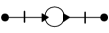
$\llbracket{\bigcirc}\rrbracket$$\quad\stackrel{{\scriptstyle\mathrm{def}}}{{=}}\quad$ $\llbracket{\mathchoice{\leavevmode\vtop{\halign{\hfil$\displaystyle#$\hfil\cr\bigcirc\cr\bullet\crcr}}}{\leavevmode\vtop{\halign{\hfil$\textstyle#$\hfil\cr\bigcirc\cr\bullet\crcr}}}{\leavevmode\vtop{\halign{\hfil$\scriptstyle#$\hfil\cr\bigcirc\cr\bullet\crcr}}}{\leavevmode\vtop{\halign{\hfil$\scriptscriptstyle#$\hfil\cr\bigcirc\cr\bullet\crcr}}}}\rrbracket$$\quad\stackrel{{\scriptstyle\mathrm{def}}}{{=}}\quad$

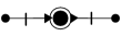
(a) C/E buffers.

$\llbracket{\mathsf{I}}\rrbracket$$\quad\stackrel{{\scriptstyle\mathrm{def}}}{{=}}\quad$ $\llbracket{\mathsf{X}}\rrbracket$$\quad\stackrel{{\scriptstyle\mathrm{def}}}{{=}}\quad$ $\llbracket{\mathsf{\Delta}}\rrbracket$$\quad\stackrel{{\scriptstyle\mathrm{def}}}{{=}}\quad$ $\llbracket{\mathchoice{{\rotatebox[origin={c}]{180.0}{$\mathsf{\Delta}$}}\displaystyle}{{\rotatebox[origin={c}]{180.0}{$\mathsf{\Delta}$}}\textstyle}{\!{\rotatebox[origin={c}]{180.0}{$\scriptstyle\mathsf{\Delta}$}}\!\scriptstyle}{{\rotatebox[origin={c}]{180.0}{$\scriptscriptstyle\mathsf{\Delta}$}}\scriptscriptstyle}}\rrbracket$$\quad\stackrel{{\scriptstyle\mathrm{def}}}{{=}}\quad$ $\llbracket{\boldsymbol{\top}}\rrbracket$$\quad\stackrel{{\scriptstyle\mathrm{def}}}{{=}}\quad$ $\llbracket{\boldsymbol{\bot}}\rrbracket$$\quad\stackrel{{\scriptstyle\mathrm{def}}}{{=}}\quad$ $\llbracket{\mathsf{\Lambda}}\rrbracket$$\quad\stackrel{{\scriptstyle\mathrm{def}}}{{=}}\quad$ $\llbracket{\mathsf{V}}\rrbracket$$\quad\stackrel{{\scriptstyle\mathrm{def}}}{{=}}\quad$ $\llbracket{\,\boldsymbol{\uparrow}\,}\rrbracket$$\quad\stackrel{{\scriptstyle\mathrm{def}}}{{=}}\quad$ $\llbracket{\,\boldsymbol{\downarrow}\,}\rrbracket$$\quad\stackrel{{\scriptstyle\mathrm{def}}}{{=}}\quad$

(b) Stateless connectors.

$\{\![\llparenthesis n\rrparenthesis]\!\}\stackrel{{\scriptstyle\mathrm{def}}}{{=}}\lower 6.0pt\hbox{\includegraphics[height=17.07182pt]{netTokensPlace}}$

(c) P/T buffers.

Figure 13. Translation from basic connectors to nets.

We start by giving a compositional translation from Petri calculus terms to C/E nets with boundaries that preserves the strong semantics in a tight manner.

Each of the basic connectors of the Petri calculus has a corresponding C/E net with the same semantics: this translation ($\llbracket{-}\rrbracket$) is given in Fig. 13(a) and Fig. 13(b), where we leave implicit that the contention relation is just the smallest relation induced by the sharing of ports. The translation extends compositionally by letting

$$\llbracket{T_{1}\mathrel{;}T_{2}}\rrbracket\stackrel{{\scriptstyle\mathrm{def}}}{{=}}\llbracket{T_{1}}\rrbracket\mathrel{;}\llbracket{T_{2}}\rrbracket\mbox{ and }\llbracket{T_{1}\otimes T_{2}}\rrbracket\stackrel{{\scriptstyle\mathrm{def}}}{{=}}\llbracket{T_{1}}\rrbracket\otimes\llbracket{T_{2}}\rrbracket.$$

We obtain a very close operational correspondence between Petri calculus terms and their translations to C/E nets, as stated by the following result.

Theorem 29.

Let $T$ be a term of the Petri calculus.

1. if $T\raise 1.0pt\hbox{$\;\mathrel{\mathop{\mathchoice{\leavevmode\vtop{\halign{\hfil$\displaystyle#$\hfil\cr\scriptstyle\xrightarrow{\,\alpha\,}\cr{\lower 1.99997pt\hbox{$\scriptstyle{}_{\beta}$}}\crcr}}}{\leavevmode\vtop{\halign{\hfil$\textstyle#$\hfil\cr\scriptstyle\xrightarrow{\,\alpha\,}\cr{\lower 1.99997pt\hbox{$\scriptstyle{}_{\beta}$}}\crcr}}}{\leavevmode\vtop{\halign{\hfil$\scriptstyle#$\hfil\cr\scriptstyle\xrightarrow{\,\alpha\,}\cr{\lower 1.39998pt\hbox{$\scriptstyle{}_{\beta}$}}\crcr}}}{\leavevmode\vtop{\halign{\hfil$\scriptscriptstyle#$\hfil\cr\scriptstyle\xrightarrow{\,\alpha\,}\cr{\lower 0.99998pt\hbox{$\scriptstyle{}_{\beta}$}}\crcr}}}}}\;$}T^{\prime}$ then $\llbracket{T}\rrbracket\raise 1.0pt\hbox{$\;\mathrel{\mathop{\mathchoice{\leavevmode\vtop{\halign{\hfil$\displaystyle#$\hfil\cr\scriptstyle\xrightarrow{\,\alpha\,}\cr{\lower 1.99997pt\hbox{$\scriptstyle{}_{\beta}$}}\crcr}}}{\leavevmode\vtop{\halign{\hfil$\textstyle#$\hfil\cr\scriptstyle\xrightarrow{\,\alpha\,}\cr{\lower 1.99997pt\hbox{$\scriptstyle{}_{\beta}$}}\crcr}}}{\leavevmode\vtop{\halign{\hfil$\scriptstyle#$\hfil\cr\scriptstyle\xrightarrow{\,\alpha\,}\cr{\lower 1.39998pt\hbox{$\scriptstyle{}_{\beta}$}}\crcr}}}{\leavevmode\vtop{\halign{\hfil$\scriptscriptstyle#$\hfil\cr\scriptstyle\xrightarrow{\,\alpha\,}\cr{\lower 0.99998pt\hbox{$\scriptstyle{}_{\beta}$}}\crcr}}}}}\;$}\llbracket{T^{\prime}}\rrbracket$.

2. if $\llbracket{T}\rrbracket\raise 1.0pt\hbox{$\;\mathrel{\mathop{\mathchoice{\leavevmode\vtop{\halign{\hfil$\displaystyle#$\hfil\cr\scriptstyle\xrightarrow{\,\alpha\,}\cr{\lower 1.99997pt\hbox{$\scriptstyle{}_{\beta}$}}\crcr}}}{\leavevmode\vtop{\halign{\hfil$\textstyle#$\hfil\cr\scriptstyle\xrightarrow{\,\alpha\,}\cr{\lower 1.99997pt\hbox{$\scriptstyle{}_{\beta}$}}\crcr}}}{\leavevmode\vtop{\halign{\hfil$\scriptstyle#$\hfil\cr\scriptstyle\xrightarrow{\,\alpha\,}\cr{\lower 1.39998pt\hbox{$\scriptstyle{}_{\beta}$}}\crcr}}}{\leavevmode\vtop{\halign{\hfil$\scriptscriptstyle#$\hfil\cr\scriptstyle\xrightarrow{\,\alpha\,}\cr{\lower 0.99998pt\hbox{$\scriptstyle{}_{\beta}$}}\crcr}}}}}\;$}N_{X}$ then there exists $T^{\prime}$ such that $T\raise 1.0pt\hbox{$\;\mathrel{\mathop{\mathchoice{\leavevmode\vtop{\halign{\hfil$\displaystyle#$\hfil\cr\scriptstyle\xrightarrow{\,\alpha\,}\cr{\lower 1.99997pt\hbox{$\scriptstyle{}_{\beta}$}}\crcr}}}{\leavevmode\vtop{\halign{\hfil$\textstyle#$\hfil\cr\scriptstyle\xrightarrow{\,\alpha\,}\cr{\lower 1.99997pt\hbox{$\scriptstyle{}_{\beta}$}}\crcr}}}{\leavevmode\vtop{\halign{\hfil$\scriptstyle#$\hfil\cr\scriptstyle\xrightarrow{\,\alpha\,}\cr{\lower 1.39998pt\hbox{$\scriptstyle{}_{\beta}$}}\crcr}}}{\leavevmode\vtop{\halign{\hfil$\scriptscriptstyle#$\hfil\cr\scriptstyle\xrightarrow{\,\alpha\,}\cr{\lower 0.99998pt\hbox{$\scriptstyle{}_{\beta}$}}\crcr}}}}}\;$}T^{\prime}$ and $\llbracket{T^{\prime}}\rrbracket=N_{X}$.

Proof 8.1.

(i) We proceed by structural induction on $T$. When $T$ is a constant, each case can be shown to hold easily by inspection of the translations illustrated in Fig. 13. Now if $T=P\mathrel{;}Q$ and $T\raise 1.0pt\hbox{$\;\mathrel{\mathop{\mathchoice{\leavevmode\vtop{\halign{\hfil$\displaystyle#$\hfil\cr\scriptstyle\xrightarrow{\,\alpha\,}\cr{\lower 1.99997pt\hbox{$\scriptstyle{}_{\beta}$}}\crcr}}}{\leavevmode\vtop{\halign{\hfil$\textstyle#$\hfil\cr\scriptstyle\xrightarrow{\,\alpha\,}\cr{\lower 1.99997pt\hbox{$\scriptstyle{}_{\beta}$}}\crcr}}}{\leavevmode\vtop{\halign{\hfil$\scriptstyle#$\hfil\cr\scriptstyle\xrightarrow{\,\alpha\,}\cr{\lower 1.39998pt\hbox{$\scriptstyle{}_{\beta}$}}\crcr}}}{\leavevmode\vtop{\halign{\hfil$\scriptscriptstyle#$\hfil\cr\scriptstyle\xrightarrow{\,\alpha\,}\cr{\lower 0.99998pt\hbox{$\scriptstyle{}_{\beta}$}}\crcr}}}}}\;$}T^{\prime}$ then we have $P\raise 1.0pt\hbox{$\;\mathrel{\mathop{\mathchoice{\leavevmode\vtop{\halign{\hfil$\displaystyle#$\hfil\cr\scriptstyle\xrightarrow{\,\alpha\,}\cr{\lower 1.99997pt\hbox{$\scriptstyle{}_{\gamma}$}}\crcr}}}{\leavevmode\vtop{\halign{\hfil$\textstyle#$\hfil\cr\scriptstyle\xrightarrow{\,\alpha\,}\cr{\lower 1.99997pt\hbox{$\scriptstyle{}_{\gamma}$}}\crcr}}}{\leavevmode\vtop{\halign{\hfil$\scriptstyle#$\hfil\cr\scriptstyle\xrightarrow{\,\alpha\,}\cr{\lower 1.39998pt\hbox{$\scriptstyle{}_{\gamma}$}}\crcr}}}{\leavevmode\vtop{\halign{\hfil$\scriptscriptstyle#$\hfil\cr\scriptstyle\xrightarrow{\,\alpha\,}\cr{\lower 0.99998pt\hbox{$\scriptstyle{}_{\gamma}$}}\crcr}}}}}\;$}P^{\prime}$, $Q\raise 1.0pt\hbox{$\;\mathrel{\mathop{\mathchoice{\leavevmode\vtop{\halign{\hfil$\displaystyle#$\hfil\cr\scriptstyle\xrightarrow{\,\gamma\,}\cr{\lower 1.99997pt\hbox{$\scriptstyle{}_{\beta}$}}\crcr}}}{\leavevmode\vtop{\halign{\hfil$\textstyle#$\hfil\cr\scriptstyle\xrightarrow{\,\gamma\,}\cr{\lower 1.99997pt\hbox{$\scriptstyle{}_{\beta}$}}\crcr}}}{\leavevmode\vtop{\halign{\hfil$\scriptstyle#$\hfil\cr\scriptstyle\xrightarrow{\,\gamma\,}\cr{\lower 1.39998pt\hbox{$\scriptstyle{}_{\beta}$}}\crcr}}}{\leavevmode\vtop{\halign{\hfil$\scriptscriptstyle#$\hfil\cr\scriptstyle\xrightarrow{\,\gamma\,}\cr{\lower 0.99998pt\hbox{$\scriptstyle{}_{\beta}$}}\crcr}}}}}\;$}Q^{\prime}$ and $T^{\prime}=P^{\prime};Q^{\prime}$. Using the inductive hypothesis we obtain $\llbracket{P}\rrbracket\raise 1.0pt\hbox{$\;\mathrel{\mathop{\mathchoice{\leavevmode\vtop{\halign{\hfil$\displaystyle#$\hfil\cr\scriptstyle\xrightarrow{\,\alpha\,}\cr{\lower 1.99997pt\hbox{$\scriptstyle{}_{\gamma}$}}\crcr}}}{\leavevmode\vtop{\halign{\hfil$\textstyle#$\hfil\cr\scriptstyle\xrightarrow{\,\alpha\,}\cr{\lower 1.99997pt\hbox{$\scriptstyle{}_{\gamma}$}}\crcr}}}{\leavevmode\vtop{\halign{\hfil$\scriptstyle#$\hfil\cr\scriptstyle\xrightarrow{\,\alpha\,}\cr{\lower 1.39998pt\hbox{$\scriptstyle{}_{\gamma}$}}\crcr}}}{\leavevmode\vtop{\halign{\hfil$\scriptscriptstyle#$\hfil\cr\scriptstyle\xrightarrow{\,\alpha\,}\cr{\lower 0.99998pt\hbox{$\scriptstyle{}_{\gamma}$}}\crcr}}}}}\;$}\llbracket{P^{\prime}}\rrbracket$ and $\llbracket{Q}\rrbracket\raise 1.0pt\hbox{$\;\mathrel{\mathop{\mathchoice{\leavevmode\vtop{\halign{\hfil$\displaystyle#$\hfil\cr\scriptstyle\xrightarrow{\,\gamma\,}\cr{\lower 1.99997pt\hbox{$\scriptstyle{}_{\beta}$}}\crcr}}}{\leavevmode\vtop{\halign{\hfil$\textstyle#$\hfil\cr\scriptstyle\xrightarrow{\,\gamma\,}\cr{\lower 1.99997pt\hbox{$\scriptstyle{}_{\beta}$}}\crcr}}}{\leavevmode\vtop{\halign{\hfil$\scriptstyle#$\hfil\cr\scriptstyle\xrightarrow{\,\gamma\,}\cr{\lower 1.39998pt\hbox{$\scriptstyle{}_{\beta}$}}\crcr}}}{\leavevmode\vtop{\halign{\hfil$\scriptscriptstyle#$\hfil\cr\scriptstyle\xrightarrow{\,\gamma\,}\cr{\lower 0.99998pt\hbox{$\scriptstyle{}_{\beta}$}}\crcr}}}}}\;$}\llbracket{Q^{\prime}}\rrbracket$. Then by Theorem 5 we obtain $\llbracket{P\mathrel{;}Q}\rrbracket=\llbracket{P}\rrbracket\mathrel{;}\llbracket{Q}\rrbracket\raise 1.0pt\hbox{$\;\mathrel{\mathop{\mathchoice{\leavevmode\vtop{\halign{\hfil$\displaystyle#$\hfil\cr\scriptstyle\xrightarrow{\,\alpha\,}\cr{\lower 1.99997pt\hbox{$\scriptstyle{}_{\beta}$}}\crcr}}}{\leavevmode\vtop{\halign{\hfil$\textstyle#$\hfil\cr\scriptstyle\xrightarrow{\,\alpha\,}\cr{\lower 1.99997pt\hbox{$\scriptstyle{}_{\beta}$}}\crcr}}}{\leavevmode\vtop{\halign{\hfil$\scriptstyle#$\hfil\cr\scriptstyle\xrightarrow{\,\alpha\,}\cr{\lower 1.39998pt\hbox{$\scriptstyle{}_{\beta}$}}\crcr}}}{\leavevmode\vtop{\halign{\hfil$\scriptscriptstyle#$\hfil\cr\scriptstyle\xrightarrow{\,\alpha\,}\cr{\lower 0.99998pt\hbox{$\scriptstyle{}_{\beta}$}}\crcr}}}}}\;$}\llbracket{P^{\prime}}\rrbracket;\llbracket{Q^{\prime}}\rrbracket=\llbracket{P^{\prime};Q^{\prime}}\rrbracket$. The case of $\otimes$ is straightforward.

(ii) Again we proceed by structural induction on $T$ and again for constants it is a matter of examination. Suppose that $T=P\mathrel{;}Q$ and $\llbracket{T}\rrbracket\raise 1.0pt\hbox{$\;\mathrel{\mathop{\mathchoice{\leavevmode\vtop{\halign{\hfil$\displaystyle#$\hfil\cr\scriptstyle\xrightarrow{\,\alpha\,}\cr{\lower 1.99997pt\hbox{$\scriptstyle{}_{\beta}$}}\crcr}}}{\leavevmode\vtop{\halign{\hfil$\textstyle#$\hfil\cr\scriptstyle\xrightarrow{\,\alpha\,}\cr{\lower 1.99997pt\hbox{$\scriptstyle{}_{\beta}$}}\crcr}}}{\leavevmode\vtop{\halign{\hfil$\scriptstyle#$\hfil\cr\scriptstyle\xrightarrow{\,\alpha\,}\cr{\lower 1.39998pt\hbox{$\scriptstyle{}_{\beta}$}}\crcr}}}{\leavevmode\vtop{\halign{\hfil$\scriptscriptstyle#$\hfil\cr\scriptstyle\xrightarrow{\,\alpha\,}\cr{\lower 0.99998pt\hbox{$\scriptstyle{}_{\beta}$}}\crcr}}}}}\;$}N_{X}$. Since $\llbracket{T}\rrbracket=\llbracket{P}\rrbracket\mathrel{;}\llbracket{Q}\rrbracket$ then by Theorem 5 there exists $\gamma$ such that $\llbracket{P}\rrbracket\raise 1.0pt\hbox{$\;\mathrel{\mathop{\mathchoice{\leavevmode\vtop{\halign{\hfil$\displaystyle#$\hfil\cr\scriptstyle\xrightarrow{\,\alpha\,}\cr{\lower 1.99997pt\hbox{$\scriptstyle{}_{\gamma}$}}\crcr}}}{\leavevmode\vtop{\halign{\hfil$\textstyle#$\hfil\cr\scriptstyle\xrightarrow{\,\alpha\,}\cr{\lower 1.99997pt\hbox{$\scriptstyle{}_{\gamma}$}}\crcr}}}{\leavevmode\vtop{\halign{\hfil$\scriptstyle#$\hfil\cr\scriptstyle\xrightarrow{\,\alpha\,}\cr{\lower 1.39998pt\hbox{$\scriptstyle{}_{\gamma}$}}\crcr}}}{\leavevmode\vtop{\halign{\hfil$\scriptscriptstyle#$\hfil\cr\scriptstyle\xrightarrow{\,\alpha\,}\cr{\lower 0.99998pt\hbox{$\scriptstyle{}_{\gamma}$}}\crcr}}}}}\;$}N^{\prime}_{X^{\prime}}$, $\llbracket{Q}\rrbracket\raise 1.0pt\hbox{$\;\mathrel{\mathop{\mathchoice{\leavevmode\vtop{\halign{\hfil$\displaystyle#$\hfil\cr\scriptstyle\xrightarrow{\,\gamma\,}\cr{\lower 1.99997pt\hbox{$\scriptstyle{}_{\beta}$}}\crcr}}}{\leavevmode\vtop{\halign{\hfil$\textstyle#$\hfil\cr\scriptstyle\xrightarrow{\,\gamma\,}\cr{\lower 1.99997pt\hbox{$\scriptstyle{}_{\beta}$}}\crcr}}}{\leavevmode\vtop{\halign{\hfil$\scriptstyle#$\hfil\cr\scriptstyle\xrightarrow{\,\gamma\,}\cr{\lower 1.39998pt\hbox{$\scriptstyle{}_{\beta}$}}\crcr}}}{\leavevmode\vtop{\halign{\hfil$\scriptscriptstyle#$\hfil\cr\scriptstyle\xrightarrow{\,\gamma\,}\cr{\lower 0.99998pt\hbox{$\scriptstyle{}_{\beta}$}}\crcr}}}}}\;$}N^{\prime\prime}_{X^{\prime\prime}}$ where $N_{X}=N^{\prime}_{X^{\prime}}\mathrel{;}N^{\prime\prime}_{X^{\prime\prime}}$. By the inductive hypothesis $P\raise 1.0pt\hbox{$\;\mathrel{\mathop{\mathchoice{\leavevmode\vtop{\halign{\hfil$\displaystyle#$\hfil\cr\scriptstyle\xrightarrow{\,\alpha\,}\cr{\lower 1.99997pt\hbox{$\scriptstyle{}_{\gamma}$}}\crcr}}}{\leavevmode\vtop{\halign{\hfil$\textstyle#$\hfil\cr\scriptstyle\xrightarrow{\,\alpha\,}\cr{\lower 1.99997pt\hbox{$\scriptstyle{}_{\gamma}$}}\crcr}}}{\leavevmode\vtop{\halign{\hfil$\scriptstyle#$\hfil\cr\scriptstyle\xrightarrow{\,\alpha\,}\cr{\lower 1.39998pt\hbox{$\scriptstyle{}_{\gamma}$}}\crcr}}}{\leavevmode\vtop{\halign{\hfil$\scriptscriptstyle#$\hfil\cr\scriptstyle\xrightarrow{\,\alpha\,}\cr{\lower 0.99998pt\hbox{$\scriptstyle{}_{\gamma}$}}\crcr}}}}}\;$}P^{\prime}$, $Q\raise 1.0pt\hbox{$\;\mathrel{\mathop{\mathchoice{\leavevmode\vtop{\halign{\hfil$\displaystyle#$\hfil\cr\scriptstyle\xrightarrow{\,\gamma\,}\cr{\lower 1.99997pt\hbox{$\scriptstyle{}_{\beta}$}}\crcr}}}{\leavevmode\vtop{\halign{\hfil$\textstyle#$\hfil\cr\scriptstyle\xrightarrow{\,\gamma\,}\cr{\lower 1.99997pt\hbox{$\scriptstyle{}_{\beta}$}}\crcr}}}{\leavevmode\vtop{\halign{\hfil$\scriptstyle#$\hfil\cr\scriptstyle\xrightarrow{\,\gamma\,}\cr{\lower 1.39998pt\hbox{$\scriptstyle{}_{\beta}$}}\crcr}}}{\leavevmode\vtop{\halign{\hfil$\scriptscriptstyle#$\hfil\cr\scriptstyle\xrightarrow{\,\gamma\,}\cr{\lower 0.99998pt\hbox{$\scriptstyle{}_{\beta}$}}\crcr}}}}}\;$}Q^{\prime}$ with $\llbracket{P^{\prime}}\rrbracket=N^{\prime}_{X^{\prime}}$ and $\llbracket{Q^{\prime}}\rrbracket=N^{\prime\prime}_{X^{\prime\prime}}$. Using (Cut) we obtain $P\mathrel{;}Q\raise 1.0pt\hbox{$\;\mathrel{\mathop{\mathchoice{\leavevmode\vtop{\halign{\hfil$\displaystyle#$\hfil\cr\scriptstyle\xrightarrow{\,\alpha\,}\cr{\lower 1.99997pt\hbox{$\scriptstyle{}_{\beta}$}}\crcr}}}{\leavevmode\vtop{\halign{\hfil$\textstyle#$\hfil\cr\scriptstyle\xrightarrow{\,\alpha\,}\cr{\lower 1.99997pt\hbox{$\scriptstyle{}_{\beta}$}}\crcr}}}{\leavevmode\vtop{\halign{\hfil$\scriptstyle#$\hfil\cr\scriptstyle\xrightarrow{\,\alpha\,}\cr{\lower 1.39998pt\hbox{$\scriptstyle{}_{\beta}$}}\crcr}}}{\leavevmode\vtop{\halign{\hfil$\scriptscriptstyle#$\hfil\cr\scriptstyle\xrightarrow{\,\alpha\,}\cr{\lower 0.99998pt\hbox{$\scriptstyle{}_{\beta}$}}\crcr}}}}}\;$}P^{\prime}\mathrel{;}Q^{\prime}$ and clearly $\llbracket{P^{\prime}\mathrel{;}Q^{\prime}}\rrbracket=\llbracket{P^{\prime}}\rrbracket\mathrel{;}\llbracket{Q^{\prime}}\rrbracket=N_{X}$. The case of $T=P\otimes Q$ is again straightforward.

8.2. Translating P/T calculus terms to P/T nets.

The translation from P/T calculus to P/T nets is similar to the translation that we have already considered. We will use the notation $\{\![-]\!\}$ to emphasise that the codomain of the translation is P/T nets, where composition of nets is defined differently. For $C$ a stateless connector, let $\{\![C]\!\}\stackrel{{\scriptstyle\mathrm{def}}}{{=}}\llbracket{C}\rrbracket$ (considered as a P/T net) as given in Fig. 13(b) and the translation of the buffers of the P/T calculus is in Fig. 13(c).

As for C/E nets, the encoding is homomorphic w.r.t. $\mathrel{;}$ and $\oplus$:

$$\{\![T_{1}\mathrel{;}T_{2}]\!\}\stackrel{{\scriptstyle\mathrm{def}}}{{=}}\{\![T_{1}]\!\}\mathrel{;}\{\![T_{2}]\!\}\mbox{ and }\{\![T_{1}\oplus T_{2}]\!\}\stackrel{{\scriptstyle\mathrm{def}}}{{=}}\{\![T_{1}]\!\}\oplus\{\![T_{2}]\!\}.$$

We first consider P/T calculus with strong semantics and P/T nets with the standard semantics.

Theorem 30.

Let $T$ be a term of P/T calculus.

1. if $T\raise 1.0pt\hbox{$\;\mathrel{\mathop{\mathchoice{\leavevmode\vtop{\halign{\hfil$\displaystyle#$\hfil\cr\scriptstyle\xrightarrow{\,\alpha\,}\cr{\lower 1.99997pt\hbox{$\scriptstyle{}_{\beta}$}}\crcr}}}{\leavevmode\vtop{\halign{\hfil$\textstyle#$\hfil\cr\scriptstyle\xrightarrow{\,\alpha\,}\cr{\lower 1.99997pt\hbox{$\scriptstyle{}_{\beta}$}}\crcr}}}{\leavevmode\vtop{\halign{\hfil$\scriptstyle#$\hfil\cr\scriptstyle\xrightarrow{\,\alpha\,}\cr{\lower 1.39998pt\hbox{$\scriptstyle{}_{\beta}$}}\crcr}}}{\leavevmode\vtop{\halign{\hfil$\scriptscriptstyle#$\hfil\cr\scriptstyle\xrightarrow{\,\alpha\,}\cr{\lower 0.99998pt\hbox{$\scriptstyle{}_{\beta}$}}\crcr}}}}}\;$}T^{\prime}$ then $\{\![T]\!\}\raise 1.0pt\hbox{$\;\mathrel{\mathop{\mathchoice{\leavevmode\vtop{\halign{\hfil$\displaystyle#$\hfil\cr\scriptstyle\xrightarrow{\,\alpha\,}\cr{\lower 1.99997pt\hbox{$\scriptstyle{}_{\beta}$}}\crcr}}}{\leavevmode\vtop{\halign{\hfil$\textstyle#$\hfil\cr\scriptstyle\xrightarrow{\,\alpha\,}\cr{\lower 1.99997pt\hbox{$\scriptstyle{}_{\beta}$}}\crcr}}}{\leavevmode\vtop{\halign{\hfil$\scriptstyle#$\hfil\cr\scriptstyle\xrightarrow{\,\alpha\,}\cr{\lower 1.39998pt\hbox{$\scriptstyle{}_{\beta}$}}\crcr}}}{\leavevmode\vtop{\halign{\hfil$\scriptscriptstyle#$\hfil\cr\scriptstyle\xrightarrow{\,\alpha\,}\cr{\lower 0.99998pt\hbox{$\scriptstyle{}_{\beta}$}}\crcr}}}}}\;$}\{\![T^{\prime}]\!\}$.

2. if $\{\![T]\!\}\raise 1.0pt\hbox{$\;\mathrel{\mathop{\mathchoice{\leavevmode\vtop{\halign{\hfil$\displaystyle#$\hfil\cr\scriptstyle\xrightarrow{\,\alpha\,}\cr{\lower 1.99997pt\hbox{$\scriptstyle{}_{\beta}$}}\crcr}}}{\leavevmode\vtop{\halign{\hfil$\textstyle#$\hfil\cr\scriptstyle\xrightarrow{\,\alpha\,}\cr{\lower 1.99997pt\hbox{$\scriptstyle{}_{\beta}$}}\crcr}}}{\leavevmode\vtop{\halign{\hfil$\scriptstyle#$\hfil\cr\scriptstyle\xrightarrow{\,\alpha\,}\cr{\lower 1.39998pt\hbox{$\scriptstyle{}_{\beta}$}}\crcr}}}{\leavevmode\vtop{\halign{\hfil$\scriptscriptstyle#$\hfil\cr\scriptstyle\xrightarrow{\,\alpha\,}\cr{\lower 0.99998pt\hbox{$\scriptstyle{}_{\beta}$}}\crcr}}}}}\;$}N_{\mathcal{X}}$ then there exists a term $T^{\prime}$ such that $T\raise 1.0pt\hbox{$\;\mathrel{\mathop{\mathchoice{\leavevmode\vtop{\halign{\hfil$\displaystyle#$\hfil\cr\scriptstyle\xrightarrow{\,\alpha\,}\cr{\lower 1.99997pt\hbox{$\scriptstyle{}_{\beta}$}}\crcr}}}{\leavevmode\vtop{\halign{\hfil$\textstyle#$\hfil\cr\scriptstyle\xrightarrow{\,\alpha\,}\cr{\lower 1.99997pt\hbox{$\scriptstyle{}_{\beta}$}}\crcr}}}{\leavevmode\vtop{\halign{\hfil$\scriptstyle#$\hfil\cr\scriptstyle\xrightarrow{\,\alpha\,}\cr{\lower 1.39998pt\hbox{$\scriptstyle{}_{\beta}$}}\crcr}}}{\leavevmode\vtop{\halign{\hfil$\scriptscriptstyle#$\hfil\cr\scriptstyle\xrightarrow{\,\alpha\,}\cr{\lower 0.99998pt\hbox{$\scriptstyle{}_{\beta}$}}\crcr}}}}}\;$}T^{\prime}$ and $\{\![T^{\prime}]\!\}=N_{\mathcal{X}}$.

Proof 8.2.

(i) We proceed by structural induction on $T$. If $T=\llparenthesis n\rrparenthesis$ then $\llparenthesis n\rrparenthesis\xrightarrow[k]{h}Q$ implies $k\leq n$ and $Q=\llparenthesis n+h-k\rrparenthesis$ by Lemma 25. Consider the net corresponding to the term $\llparenthesis n\rrparenthesis$ given in Fig. 13(c) and let $\alpha$ be the transition on the left and $\beta$ the transition on the right. Take $\mathcal{U}=h\alpha+k\beta$. It is immediate to check that $\{\![T]\!\}\rightarrow_{\mathcal{U}}\{\![\llparenthesis n+h-k\rrparenthesis]\!\}$. The cases corresponding to the remaining constants can be shown to hold easily by inspection of the translations illustrated in Fig. 13. Now if $T=T_{1};T_{2}$ and $T\raise 1.0pt\hbox{$\;\mathrel{\mathop{\mathchoice{\leavevmode\vtop{\halign{\hfil$\displaystyle#$\hfil\cr\scriptstyle\xrightarrow{\,\alpha\,}\cr{\lower 1.99997pt\hbox{$\scriptstyle{}_{\beta}$}}\crcr}}}{\leavevmode\vtop{\halign{\hfil$\textstyle#$\hfil\cr\scriptstyle\xrightarrow{\,\alpha\,}\cr{\lower 1.99997pt\hbox{$\scriptstyle{}_{\beta}$}}\crcr}}}{\leavevmode\vtop{\halign{\hfil$\scriptstyle#$\hfil\cr\scriptstyle\xrightarrow{\,\alpha\,}\cr{\lower 1.39998pt\hbox{$\scriptstyle{}_{\beta}$}}\crcr}}}{\leavevmode\vtop{\halign{\hfil$\scriptscriptstyle#$\hfil\cr\scriptstyle\xrightarrow{\,\alpha\,}\cr{\lower 0.99998pt\hbox{$\scriptstyle{}_{\beta}$}}\crcr}}}}}\;$}T^{\prime}$ then we have $T_{1}\raise 1.0pt\hbox{$\;\mathrel{\mathop{\mathchoice{\leavevmode\vtop{\halign{\hfil$\displaystyle#$\hfil\cr\scriptstyle\xrightarrow{\,\alpha\,}\cr{\lower 1.99997pt\hbox{$\scriptstyle{}_{\gamma}$}}\crcr}}}{\leavevmode\vtop{\halign{\hfil$\textstyle#$\hfil\cr\scriptstyle\xrightarrow{\,\alpha\,}\cr{\lower 1.99997pt\hbox{$\scriptstyle{}_{\gamma}$}}\crcr}}}{\leavevmode\vtop{\halign{\hfil$\scriptstyle#$\hfil\cr\scriptstyle\xrightarrow{\,\alpha\,}\cr{\lower 1.39998pt\hbox{$\scriptstyle{}_{\gamma}$}}\crcr}}}{\leavevmode\vtop{\halign{\hfil$\scriptscriptstyle#$\hfil\cr\scriptstyle\xrightarrow{\,\alpha\,}\cr{\lower 0.99998pt\hbox{$\scriptstyle{}_{\gamma}$}}\crcr}}}}}\;$}T_{1}^{\prime}$, $T_{2}\raise 1.0pt\hbox{$\;\mathrel{\mathop{\mathchoice{\leavevmode\vtop{\halign{\hfil$\displaystyle#$\hfil\cr\scriptstyle\xrightarrow{\,\gamma\,}\cr{\lower 1.99997pt\hbox{$\scriptstyle{}_{\beta}$}}\crcr}}}{\leavevmode\vtop{\halign{\hfil$\textstyle#$\hfil\cr\scriptstyle\xrightarrow{\,\gamma\,}\cr{\lower 1.99997pt\hbox{$\scriptstyle{}_{\beta}$}}\crcr}}}{\leavevmode\vtop{\halign{\hfil$\scriptstyle#$\hfil\cr\scriptstyle\xrightarrow{\,\gamma\,}\cr{\lower 1.39998pt\hbox{$\scriptstyle{}_{\beta}$}}\crcr}}}{\leavevmode\vtop{\halign{\hfil$\scriptscriptstyle#$\hfil\cr\scriptstyle\xrightarrow{\,\gamma\,}\cr{\lower 0.99998pt\hbox{$\scriptstyle{}_{\beta}$}}\crcr}}}}}\;$}T_{2}^{\prime}$ and $T^{\prime}=T_{1}^{\prime};T_{2}^{\prime}$. Using the inductive hypothesis we obtain $\{\![T_{1}]\!\}\raise 1.0pt\hbox{$\;\mathrel{\mathop{\mathchoice{\leavevmode\vtop{\halign{\hfil$\displaystyle#$\hfil\cr\scriptstyle\xrightarrow{\,\alpha\,}\cr{\lower 1.99997pt\hbox{$\scriptstyle{}_{\gamma}$}}\crcr}}}{\leavevmode\vtop{\halign{\hfil$\textstyle#$\hfil\cr\scriptstyle\xrightarrow{\,\alpha\,}\cr{\lower 1.99997pt\hbox{$\scriptstyle{}_{\gamma}$}}\crcr}}}{\leavevmode\vtop{\halign{\hfil$\scriptstyle#$\hfil\cr\scriptstyle\xrightarrow{\,\alpha\,}\cr{\lower 1.39998pt\hbox{$\scriptstyle{}_{\gamma}$}}\crcr}}}{\leavevmode\vtop{\halign{\hfil$\scriptscriptstyle#$\hfil\cr\scriptstyle\xrightarrow{\,\alpha\,}\cr{\lower 0.99998pt\hbox{$\scriptstyle{}_{\gamma}$}}\crcr}}}}}\;$}\{\![T_{1}^{\prime}]\!\}$ and $\{\![T_{2}]\!\}\raise 1.0pt\hbox{$\;\mathrel{\mathop{\mathchoice{\leavevmode\vtop{\halign{\hfil$\displaystyle#$\hfil\cr\scriptstyle\xrightarrow{\,\gamma\,}\cr{\lower 1.99997pt\hbox{$\scriptstyle{}_{\beta}$}}\crcr}}}{\leavevmode\vtop{\halign{\hfil$\textstyle#$\hfil\cr\scriptstyle\xrightarrow{\,\gamma\,}\cr{\lower 1.99997pt\hbox{$\scriptstyle{}_{\beta}$}}\crcr}}}{\leavevmode\vtop{\halign{\hfil$\scriptstyle#$\hfil\cr\scriptstyle\xrightarrow{\,\gamma\,}\cr{\lower 1.39998pt\hbox{$\scriptstyle{}_{\beta}$}}\crcr}}}{\leavevmode\vtop{\halign{\hfil$\scriptscriptstyle#$\hfil\cr\scriptstyle\xrightarrow{\,\gamma\,}\cr{\lower 0.99998pt\hbox{$\scriptstyle{}_{\beta}$}}\crcr}}}}}\;$}\{\![T_{2}^{\prime}]\!\}$. By Theorem 12($i$),

$$\{\![T_{1};T_{2}]\!\}=\{\![T_{1}]\!\};\{\![T_{2}]\!\}\raise 1.0pt\hbox{$\;\mathrel{\mathop{\mathchoice{\leavevmode\vtop{\halign{\hfil$\displaystyle#$\hfil\cr\scriptstyle\xrightarrow{\,\alpha\,}\cr{\lower 1.99997pt\hbox{$\scriptstyle{}_{\beta}$}}\crcr}}}{\leavevmode\vtop{\halign{\hfil$\textstyle#$\hfil\cr\scriptstyle\xrightarrow{\,\alpha\,}\cr{\lower 1.99997pt\hbox{$\scriptstyle{}_{\beta}$}}\crcr}}}{\leavevmode\vtop{\halign{\hfil$\scriptstyle#$\hfil\cr\scriptstyle\xrightarrow{\,\alpha\,}\cr{\lower 1.39998pt\hbox{$\scriptstyle{}_{\beta}$}}\crcr}}}{\leavevmode\vtop{\halign{\hfil$\scriptscriptstyle#$\hfil\cr\scriptstyle\xrightarrow{\,\alpha\,}\cr{\lower 0.99998pt\hbox{$\scriptstyle{}_{\beta}$}}\crcr}}}}}\;$}\{\![T_{1}^{\prime}]\!\};\{\![T_{2}^{\prime}]\!\}=\{\![T_{1}^{\prime};T_{2}^{\prime}]\!\}.$$

The case for $\otimes$ follows by using rule (ten), inductive hypothesis on both premises and then parallel composition of nets.

(ii) Again we proceed by structural induction on $T$ and again for constants it is a matter of examination. Suppose that $T=T_{1};T_{2}$ and $\{\![T]\!\}\raise 1.0pt\hbox{$\;\mathrel{\mathop{\mathchoice{\leavevmode\vtop{\halign{\hfil$\displaystyle#$\hfil\cr\scriptstyle\xrightarrow{\,\alpha\,}\cr{\lower 1.99997pt\hbox{$\scriptstyle{}_{\beta}$}}\crcr}}}{\leavevmode\vtop{\halign{\hfil$\textstyle#$\hfil\cr\scriptstyle\xrightarrow{\,\alpha\,}\cr{\lower 1.99997pt\hbox{$\scriptstyle{}_{\beta}$}}\crcr}}}{\leavevmode\vtop{\halign{\hfil$\scriptstyle#$\hfil\cr\scriptstyle\xrightarrow{\,\alpha\,}\cr{\lower 1.39998pt\hbox{$\scriptstyle{}_{\beta}$}}\crcr}}}{\leavevmode\vtop{\halign{\hfil$\scriptscriptstyle#$\hfil\cr\scriptstyle\xrightarrow{\,\alpha\,}\cr{\lower 0.99998pt\hbox{$\scriptstyle{}_{\beta}$}}\crcr}}}}}\;$}N_{\mathcal{X}}$. Then, $\{\![T]\!\}=\{\![T_{1}]\!\};\{\![T_{2}]\!\}$ by definition of the encoding. By Theorem 12($i$), there exists $\gamma$ such that $\{\![T_{1}]\!\}\raise 1.0pt\hbox{$\;\mathrel{\mathop{\mathchoice{\leavevmode\vtop{\halign{\hfil$\displaystyle#$\hfil\cr\scriptstyle\xrightarrow{\,\alpha\,}\cr{\lower 1.99997pt\hbox{$\scriptstyle{}_{\gamma}$}}\crcr}}}{\leavevmode\vtop{\halign{\hfil$\textstyle#$\hfil\cr\scriptstyle\xrightarrow{\,\alpha\,}\cr{\lower 1.99997pt\hbox{$\scriptstyle{}_{\gamma}$}}\crcr}}}{\leavevmode\vtop{\halign{\hfil$\scriptstyle#$\hfil\cr\scriptstyle\xrightarrow{\,\alpha\,}\cr{\lower 1.39998pt\hbox{$\scriptstyle{}_{\gamma}$}}\crcr}}}{\leavevmode\vtop{\halign{\hfil$\scriptscriptstyle#$\hfil\cr\scriptstyle\xrightarrow{\,\alpha\,}\cr{\lower 0.99998pt\hbox{$\scriptstyle{}_{\gamma}$}}\crcr}}}}}\;$}{N_{1\mathcal{X}_{1}}}$, $\{\![T_{2}]\!\}\raise 1.0pt\hbox{$\;\mathrel{\mathop{\mathchoice{\leavevmode\vtop{\halign{\hfil$\displaystyle#$\hfil\cr\scriptstyle\xrightarrow{\,\gamma\,}\cr{\lower 1.99997pt\hbox{$\scriptstyle{}_{\beta}$}}\crcr}}}{\leavevmode\vtop{\halign{\hfil$\textstyle#$\hfil\cr\scriptstyle\xrightarrow{\,\gamma\,}\cr{\lower 1.99997pt\hbox{$\scriptstyle{}_{\beta}$}}\crcr}}}{\leavevmode\vtop{\halign{\hfil$\scriptstyle#$\hfil\cr\scriptstyle\xrightarrow{\,\gamma\,}\cr{\lower 1.39998pt\hbox{$\scriptstyle{}_{\beta}$}}\crcr}}}{\leavevmode\vtop{\halign{\hfil$\scriptscriptstyle#$\hfil\cr\scriptstyle\xrightarrow{\,\gamma\,}\cr{\lower 0.99998pt\hbox{$\scriptstyle{}_{\beta}$}}\crcr}}}}}\;$}{N_{2\mathcal{X}_{2}}}$. By the inductive hypothesis $T_{1}\raise 1.0pt\hbox{$\;\mathrel{\mathop{\mathchoice{\leavevmode\vtop{\halign{\hfil$\displaystyle#$\hfil\cr\scriptstyle\xrightarrow{\,\alpha\,}\cr{\lower 1.99997pt\hbox{$\scriptstyle{}_{\gamma}$}}\crcr}}}{\leavevmode\vtop{\halign{\hfil$\textstyle#$\hfil\cr\scriptstyle\xrightarrow{\,\alpha\,}\cr{\lower 1.99997pt\hbox{$\scriptstyle{}_{\gamma}$}}\crcr}}}{\leavevmode\vtop{\halign{\hfil$\scriptstyle#$\hfil\cr\scriptstyle\xrightarrow{\,\alpha\,}\cr{\lower 1.39998pt\hbox{$\scriptstyle{}_{\gamma}$}}\crcr}}}{\leavevmode\vtop{\halign{\hfil$\scriptscriptstyle#$\hfil\cr\scriptstyle\xrightarrow{\,\alpha\,}\cr{\lower 0.99998pt\hbox{$\scriptstyle{}_{\gamma}$}}\crcr}}}}}\;$}T_{1}^{\prime}$, $T_{2}\raise 1.0pt\hbox{$\;\mathrel{\mathop{\mathchoice{\leavevmode\vtop{\halign{\hfil$\displaystyle#$\hfil\cr\scriptstyle\xrightarrow{\,\gamma\,}\cr{\lower 1.99997pt\hbox{$\scriptstyle{}_{\beta}$}}\crcr}}}{\leavevmode\vtop{\halign{\hfil$\textstyle#$\hfil\cr\scriptstyle\xrightarrow{\,\gamma\,}\cr{\lower 1.99997pt\hbox{$\scriptstyle{}_{\beta}$}}\crcr}}}{\leavevmode\vtop{\halign{\hfil$\scriptstyle#$\hfil\cr\scriptstyle\xrightarrow{\,\gamma\,}\cr{\lower 1.39998pt\hbox{$\scriptstyle{}_{\beta}$}}\crcr}}}{\leavevmode\vtop{\halign{\hfil$\scriptscriptstyle#$\hfil\cr\scriptstyle\xrightarrow{\,\gamma\,}\cr{\lower 0.99998pt\hbox{$\scriptstyle{}_{\beta}$}}\crcr}}}}}\;$}T_{2}^{\prime}$ with $\{\![T_{1}^{\prime}]\!\}={N_{1\mathcal{X}_{1}}}$ and $\{\![T_{2}^{\prime}]\!\}={N_{2\mathcal{X}_{2}}}$. Using (Cut) we obtain $T_{1};T_{2}\raise 1.0pt\hbox{$\;\mathrel{\mathop{\mathchoice{\leavevmode\vtop{\halign{\hfil$\displaystyle#$\hfil\cr\scriptstyle\xrightarrow{\,\alpha\,}\cr{\lower 1.99997pt\hbox{$\scriptstyle{}_{\beta}$}}\crcr}}}{\leavevmode\vtop{\halign{\hfil$\textstyle#$\hfil\cr\scriptstyle\xrightarrow{\,\alpha\,}\cr{\lower 1.99997pt\hbox{$\scriptstyle{}_{\beta}$}}\crcr}}}{\leavevmode\vtop{\halign{\hfil$\scriptstyle#$\hfil\cr\scriptstyle\xrightarrow{\,\alpha\,}\cr{\lower 1.39998pt\hbox{$\scriptstyle{}_{\beta}$}}\crcr}}}{\leavevmode\vtop{\halign{\hfil$\scriptscriptstyle#$\hfil\cr\scriptstyle\xrightarrow{\,\alpha\,}\cr{\lower 0.99998pt\hbox{$\scriptstyle{}_{\beta}$}}\crcr}}}}}\;$}T_{1}^{\prime};T_{2}^{\prime}$ and clearly $\{\![T_{1}^{\prime};T_{2}^{\prime}]\!\}=\{\![T_{1}^{\prime}]\!\};\{\![T_{2}^{\prime}]\!\}=(N_{1};N_{2})_{\mathcal{X}}$ where $\mathcal{X}=\mathcal{X}_{1}+\mathcal{X}_{2}$.

Then, we extend the result to P/T calculus and P/T nets with weak semantics.

Theorem 31.

Let $T$ be a term of P/T calculus.

1. if $T\raise 1.0pt\hbox{$\;\mathrel{\mathop{\mathchoice{\leavevmode\vtop{\halign{\hfil$\displaystyle#$\hfil\cr\scriptstyle\Longrightarrow\cr{\lower-6.00006pt\hbox{$\scriptstyle{}_{\alpha}$}}\cr{\lower 3.00003pt\hbox{$\scriptstyle{}_{\beta}$}}\crcr}}}{\leavevmode\vtop{\halign{\hfil$\textstyle#$\hfil\cr\scriptstyle\Longrightarrow\cr{\lower-6.00006pt\hbox{$\scriptstyle{}_{\alpha}$}}\cr{\lower 3.00003pt\hbox{$\scriptstyle{}_{\beta}$}}\crcr}}}{\leavevmode\vtop{\halign{\hfil$\scriptstyle#$\hfil\cr\scriptstyle\Longrightarrow\cr{\lower-4.20004pt\hbox{$\scriptstyle{}_{\alpha}$}}\cr{\lower 2.10002pt\hbox{$\scriptstyle{}_{\beta}$}}\crcr}}}{\leavevmode\vtop{\halign{\hfil$\scriptscriptstyle#$\hfil\cr\scriptstyle\Longrightarrow\cr{\lower-3.00003pt\hbox{$\scriptstyle{}_{\alpha}$}}\cr{\lower 1.50002pt\hbox{$\scriptstyle{}_{\beta}$}}\crcr}}}}}\;$}T^{\prime}$ then $\{\![T]\!\}\raise 1.0pt\hbox{$\;\mathrel{\mathop{\mathchoice{\leavevmode\vtop{\halign{\hfil$\displaystyle#$\hfil\cr\scriptstyle\Longrightarrow\cr{\lower-6.00006pt\hbox{$\scriptstyle{}_{\alpha}$}}\cr{\lower 3.00003pt\hbox{$\scriptstyle{}_{\beta}$}}\crcr}}}{\leavevmode\vtop{\halign{\hfil$\textstyle#$\hfil\cr\scriptstyle\Longrightarrow\cr{\lower-6.00006pt\hbox{$\scriptstyle{}_{\alpha}$}}\cr{\lower 3.00003pt\hbox{$\scriptstyle{}_{\beta}$}}\crcr}}}{\leavevmode\vtop{\halign{\hfil$\scriptstyle#$\hfil\cr\scriptstyle\Longrightarrow\cr{\lower-4.20004pt\hbox{$\scriptstyle{}_{\alpha}$}}\cr{\lower 2.10002pt\hbox{$\scriptstyle{}_{\beta}$}}\crcr}}}{\leavevmode\vtop{\halign{\hfil$\scriptscriptstyle#$\hfil\cr\scriptstyle\Longrightarrow\cr{\lower-3.00003pt\hbox{$\scriptstyle{}_{\alpha}$}}\cr{\lower 1.50002pt\hbox{$\scriptstyle{}_{\beta}$}}\crcr}}}}}\;$}\{\![T^{\prime}]\!\}$.

2. if $\{\![T]\!\}\raise 1.0pt\hbox{$\;\mathrel{\mathop{\mathchoice{\leavevmode\vtop{\halign{\hfil$\displaystyle#$\hfil\cr\scriptstyle\Longrightarrow\cr{\lower-6.00006pt\hbox{$\scriptstyle{}_{\alpha}$}}\cr{\lower 3.00003pt\hbox{$\scriptstyle{}_{\beta}$}}\crcr}}}{\leavevmode\vtop{\halign{\hfil$\textstyle#$\hfil\cr\scriptstyle\Longrightarrow\cr{\lower-6.00006pt\hbox{$\scriptstyle{}_{\alpha}$}}\cr{\lower 3.00003pt\hbox{$\scriptstyle{}_{\beta}$}}\crcr}}}{\leavevmode\vtop{\halign{\hfil$\scriptstyle#$\hfil\cr\scriptstyle\Longrightarrow\cr{\lower-4.20004pt\hbox{$\scriptstyle{}_{\alpha}$}}\cr{\lower 2.10002pt\hbox{$\scriptstyle{}_{\beta}$}}\crcr}}}{\leavevmode\vtop{\halign{\hfil$\scriptscriptstyle#$\hfil\cr\scriptstyle\Longrightarrow\cr{\lower-3.00003pt\hbox{$\scriptstyle{}_{\alpha}$}}\cr{\lower 1.50002pt\hbox{$\scriptstyle{}_{\beta}$}}\crcr}}}}}\;$}{N_{\mathcal{X}}}$ then there exists a term $T^{\prime}$ such that $T\raise 1.0pt\hbox{$\;\mathrel{\mathop{\mathchoice{\leavevmode\vtop{\halign{\hfil$\displaystyle#$\hfil\cr\scriptstyle\Longrightarrow\cr{\lower-6.00006pt\hbox{$\scriptstyle{}_{\alpha}$}}\cr{\lower 3.00003pt\hbox{$\scriptstyle{}_{\beta}$}}\crcr}}}{\leavevmode\vtop{\halign{\hfil$\textstyle#$\hfil\cr\scriptstyle\Longrightarrow\cr{\lower-6.00006pt\hbox{$\scriptstyle{}_{\alpha}$}}\cr{\lower 3.00003pt\hbox{$\scriptstyle{}_{\beta}$}}\crcr}}}{\leavevmode\vtop{\halign{\hfil$\scriptstyle#$\hfil\cr\scriptstyle\Longrightarrow\cr{\lower-4.20004pt\hbox{$\scriptstyle{}_{\alpha}$}}\cr{\lower 2.10002pt\hbox{$\scriptstyle{}_{\beta}$}}\crcr}}}{\leavevmode\vtop{\halign{\hfil$\scriptscriptstyle#$\hfil\cr\scriptstyle\Longrightarrow\cr{\lower-3.00003pt\hbox{$\scriptstyle{}_{\alpha}$}}\cr{\lower 1.50002pt\hbox{$\scriptstyle{}_{\beta}$}}\crcr}}}}}\;$}T^{\prime}$ and $\{\![T^{\prime}]\!\}={N_{\mathcal{X}}}$.

Proof 8.3.

The proof follows analogously to the one of Theorem 30 (for this case we rely on Lemma 26 and Theorem 12 ($ii$)).

To complete the picture, we also give a translation of Petri calculus terms with weak semantics to weak C/E nets, that is P/T nets with banking semantics where the marking is a subset (instead of a multiset) of places. Again, the translation of basic connectors is defined as in Fig. 13, and the translation of compound terms is homomorphic. The proof is similar to the proof of Theorem 31 (this is in particular due to the fact that in Theorem 12 if $\mathcal{X}$ and $\mathcal{Y}$ are sets, so are $\mathcal{X}_{M}$, $\mathcal{X}_{N}$, $\mathcal{Y}_{M}$, and $\mathcal{Y}_{N}$).

Proposition 32.

Let $T$ be a term of the Petri calculus.

1. if $T\raise 1.0pt\hbox{$\;\mathrel{\mathop{\mathchoice{\leavevmode\vtop{\halign{\hfil$\displaystyle#$\hfil\cr\scriptstyle\Longrightarrow\cr{\lower-6.00006pt\hbox{$\scriptstyle{}_{\alpha}$}}\cr{\lower 3.00003pt\hbox{$\scriptstyle{}_{\beta}$}}\crcr}}}{\leavevmode\vtop{\halign{\hfil$\textstyle#$\hfil\cr\scriptstyle\Longrightarrow\cr{\lower-6.00006pt\hbox{$\scriptstyle{}_{\alpha}$}}\cr{\lower 3.00003pt\hbox{$\scriptstyle{}_{\beta}$}}\crcr}}}{\leavevmode\vtop{\halign{\hfil$\scriptstyle#$\hfil\cr\scriptstyle\Longrightarrow\cr{\lower-4.20004pt\hbox{$\scriptstyle{}_{\alpha}$}}\cr{\lower 2.10002pt\hbox{$\scriptstyle{}_{\beta}$}}\crcr}}}{\leavevmode\vtop{\halign{\hfil$\scriptscriptstyle#$\hfil\cr\scriptstyle\Longrightarrow\cr{\lower-3.00003pt\hbox{$\scriptstyle{}_{\alpha}$}}\cr{\lower 1.50002pt\hbox{$\scriptstyle{}_{\beta}$}}\crcr}}}}}\;$}T^{\prime}$ then $\{\![T]\!\}\raise 1.0pt\hbox{$\;\mathrel{\mathop{\mathchoice{\leavevmode\vtop{\halign{\hfil$\displaystyle#$\hfil\cr\scriptstyle\Longrightarrow\cr{\lower-6.00006pt\hbox{$\scriptstyle{}_{\alpha}$}}\cr{\lower 3.00003pt\hbox{$\scriptstyle{}_{\beta}$}}\crcr}}}{\leavevmode\vtop{\halign{\hfil$\textstyle#$\hfil\cr\scriptstyle\Longrightarrow\cr{\lower-6.00006pt\hbox{$\scriptstyle{}_{\alpha}$}}\cr{\lower 3.00003pt\hbox{$\scriptstyle{}_{\beta}$}}\crcr}}}{\leavevmode\vtop{\halign{\hfil$\scriptstyle#$\hfil\cr\scriptstyle\Longrightarrow\cr{\lower-4.20004pt\hbox{$\scriptstyle{}_{\alpha}$}}\cr{\lower 2.10002pt\hbox{$\scriptstyle{}_{\beta}$}}\crcr}}}{\leavevmode\vtop{\halign{\hfil$\scriptscriptstyle#$\hfil\cr\scriptstyle\Longrightarrow\cr{\lower-3.00003pt\hbox{$\scriptstyle{}_{\alpha}$}}\cr{\lower 1.50002pt\hbox{$\scriptstyle{}_{\beta}$}}\crcr}}}}}\;$}\{\![T^{\prime}]\!\}$.

2. if $\{\![T]\!\}\raise 1.0pt\hbox{$\;\mathrel{\mathop{\mathchoice{\leavevmode\vtop{\halign{\hfil$\displaystyle#$\hfil\cr\scriptstyle\Longrightarrow\cr{\lower-6.00006pt\hbox{$\scriptstyle{}_{\alpha}$}}\cr{\lower 3.00003pt\hbox{$\scriptstyle{}_{\beta}$}}\crcr}}}{\leavevmode\vtop{\halign{\hfil$\textstyle#$\hfil\cr\scriptstyle\Longrightarrow\cr{\lower-6.00006pt\hbox{$\scriptstyle{}_{\alpha}$}}\cr{\lower 3.00003pt\hbox{$\scriptstyle{}_{\beta}$}}\crcr}}}{\leavevmode\vtop{\halign{\hfil$\scriptstyle#$\hfil\cr\scriptstyle\Longrightarrow\cr{\lower-4.20004pt\hbox{$\scriptstyle{}_{\alpha}$}}\cr{\lower 2.10002pt\hbox{$\scriptstyle{}_{\beta}$}}\crcr}}}{\leavevmode\vtop{\halign{\hfil$\scriptscriptstyle#$\hfil\cr\scriptstyle\Longrightarrow\cr{\lower-3.00003pt\hbox{$\scriptstyle{}_{\alpha}$}}\cr{\lower 1.50002pt\hbox{$\scriptstyle{}_{\beta}$}}\crcr}}}}}\;$}N_{X}$ then there exists $T^{\prime}$ such that $T\raise 1.0pt\hbox{$\;\mathrel{\mathop{\mathchoice{\leavevmode\vtop{\halign{\hfil$\displaystyle#$\hfil\cr\scriptstyle\Longrightarrow\cr{\lower-6.00006pt\hbox{$\scriptstyle{}_{\alpha}$}}\cr{\lower 3.00003pt\hbox{$\scriptstyle{}_{\beta}$}}\crcr}}}{\leavevmode\vtop{\halign{\hfil$\textstyle#$\hfil\cr\scriptstyle\Longrightarrow\cr{\lower-6.00006pt\hbox{$\scriptstyle{}_{\alpha}$}}\cr{\lower 3.00003pt\hbox{$\scriptstyle{}_{\beta}$}}\crcr}}}{\leavevmode\vtop{\halign{\hfil$\scriptstyle#$\hfil\cr\scriptstyle\Longrightarrow\cr{\lower-4.20004pt\hbox{$\scriptstyle{}_{\alpha}$}}\cr{\lower 2.10002pt\hbox{$\scriptstyle{}_{\beta}$}}\crcr}}}{\leavevmode\vtop{\halign{\hfil$\scriptscriptstyle#$\hfil\cr\scriptstyle\Longrightarrow\cr{\lower-3.00003pt\hbox{$\scriptstyle{}_{\alpha}$}}\cr{\lower 1.50002pt\hbox{$\scriptstyle{}_{\beta}$}}\crcr}}}}}\;$}T^{\prime}$ and $\{\![T^{\prime}]\!\}=N_{X}$.

9. Translating nets to terms

In this section we exhibit translations from the net models to process algebra terms. As with the translations in Section 8 all the translations preserve and reflect semantics. Concretely, we will define translations:

1. from C/E nets to Petri calculus terms with strong semantics (Theorem 37);

2. from weak C/E nets (see Remark 9) to Petri calculus terms with weak semantics (Theorem 40);

3. from P/T nets with standard semantics to P/T calculus terms with strong semantics (Theorem 42);

4. from P/T nets with the banking semantics to P/T calculus terms with weak semantics (Theorem 43).

First we treat the translation from C/E nets to Petri calculus terms. In order to do this we shall need to first introduce and study particular kinds of Petri calculus terms: relational forms (Definition 9.2). In order to translate P/T nets, these will be later generalised to multirelational forms (Definition 9.6), which are relevant in the Petri calculus with weak semantics and the two variants of the P/T calculus. These building blocks allow us to translate any net with boundary to a corresponding process algebra term with the same labelled semantics.

Relational and multirelational forms are built from more basic syntactic building blocks: inverse functional forms (Definition 9.1), direct functional forms (Definition 14), and additionally for multirelational forms, amplifiers (Definition 9.5). For $\Theta$ a set of Petri calculus terms, let $T_{\Theta}$ denote the set of terms generated by the following grammar:

$$T_{\Theta}\;::=\;\theta\in\Theta\;\;|\;\;\mathsf{I}\;\;|\;\;T_{\Theta}\otimes T_{\Theta}\;\;|\;\;T_{\Theta}\mathrel{;}T_{\Theta}.$$

We shall use $t_{\Theta}$ to range over terms of $T_{\Theta}$.

9.1. Functional forms

We start by introducing functional forms, which are instrumental to the definition of the relational forms used in the proposed encoding.

[Inverse functional form] A term $t\mathrel{:}(k,\,l)$ is said to be in right inverse functional form when it is in $T_{\{\boldsymbol{\bot}\}}\mathrel{;}T_{\{\mathsf{\Delta}\}}\mathrel{;}T_{\{\mathsf{X}\}}$. Dually, $t\mathrel{:}(k,\,l)$ is in left inverse functional form when it is in $T_{\{\mathsf{X}\}}\mathrel{;}T_{\{\mathchoice{{\rotatebox[origin={c}]{180.0}{$\mathsf{\Delta}$}}\displaystyle}{{\rotatebox[origin={c}]{180.0}{$\mathsf{\Delta}$}}\textstyle}{\!{\rotatebox[origin={c}]{180.0}{$\scriptstyle\mathsf{\Delta}$}}\!\scriptstyle}{{\rotatebox[origin={c}]{180.0}{$\scriptscriptstyle\mathsf{\Delta}$}}\scriptscriptstyle}\}}\mathrel{;}T_{\{\boldsymbol{\top}\}}$.

Lemma 33.

For any function $f\colon\underline{l}\to\underline{k}$ there exists a term $\mathrm{riff}_{f}\mathrel{:}(k,\,l)$ in right inverse functional form, the dynamics of which are characterised by the following:

$$\mathrm{riff}_{f}\raise 1.0pt\hbox{$\;\mathrel{\mathop{\mathchoice{\leavevmode\vtop{\halign{\hfil$\displaystyle#$\hfil\cr\scriptstyle\xrightarrow{\,\alpha\,}\cr{\lower 1.99997pt\hbox{$\scriptstyle{}_{\beta}$}}\crcr}}}{\leavevmode\vtop{\halign{\hfil$\textstyle#$\hfil\cr\scriptstyle\xrightarrow{\,\alpha\,}\cr{\lower 1.99997pt\hbox{$\scriptstyle{}_{\beta}$}}\crcr}}}{\leavevmode\vtop{\halign{\hfil$\scriptstyle#$\hfil\cr\scriptstyle\xrightarrow{\,\alpha\,}\cr{\lower 1.39998pt\hbox{$\scriptstyle{}_{\beta}$}}\crcr}}}{\leavevmode\vtop{\halign{\hfil$\scriptscriptstyle#$\hfil\cr\scriptstyle\xrightarrow{\,\alpha\,}\cr{\lower 0.99998pt\hbox{$\scriptstyle{}_{\beta}$}}\crcr}}}}}\;$}\mathrm{riff}_{f}\ \Leftrightarrow\ \exists U\subseteq\underline{k}\mbox{ s.t. }\alpha={\ulcorner U\urcorner}\mbox{ and }\beta={\ulcorner f^{-1}(U)\urcorner}$$

$$\mathrm{riff}_{f}\raise 1.0pt\hbox{$\;\mathrel{\mathop{\mathchoice{\leavevmode\vtop{\halign{\hfil$\displaystyle#$\hfil\cr\scriptstyle\Longrightarrow\cr{\lower-6.00006pt\hbox{$\scriptstyle{}_{\alpha}$}}\cr{\lower 3.00003pt\hbox{$\scriptstyle{}_{\beta}$}}\crcr}}}{\leavevmode\vtop{\halign{\hfil$\textstyle#$\hfil\cr\scriptstyle\Longrightarrow\cr{\lower-6.00006pt\hbox{$\scriptstyle{}_{\alpha}$}}\cr{\lower 3.00003pt\hbox{$\scriptstyle{}_{\beta}$}}\crcr}}}{\leavevmode\vtop{\halign{\hfil$\scriptstyle#$\hfil\cr\scriptstyle\Longrightarrow\cr{\lower-4.20004pt\hbox{$\scriptstyle{}_{\alpha}$}}\cr{\lower 2.10002pt\hbox{$\scriptstyle{}_{\beta}$}}\crcr}}}{\leavevmode\vtop{\halign{\hfil$\scriptscriptstyle#$\hfil\cr\scriptstyle\Longrightarrow\cr{\lower-3.00003pt\hbox{$\scriptstyle{}_{\alpha}$}}\cr{\lower 1.50002pt\hbox{$\scriptstyle{}_{\beta}$}}\crcr}}}}}\;$}\mathrm{riff}_{f}\ \Leftrightarrow\ \exists\mathcal{U}\in\mathcal{M}_{\underline{k}}\mbox{ s.t. }\alpha={\ulcorner\mathcal{U}\urcorner}\mbox{ and }\beta={\ulcorner f^{-1}(\mathcal{U})\urcorner}$$

The symmetric result holds for terms $t\mathrel{:}(l,\,k)$ in left inverse functional form. That is, given a function $f\colon\underline{l}\to\underline{k}$ there exists a term $\mathrm{liff}_{f}\mathrel{:}(l,\,k)$ in left inverse functional form, the dynamics of which are characterised by the following:

$$\mathrm{liff}_{f}\raise 1.0pt\hbox{$\;\mathrel{\mathop{\mathchoice{\leavevmode\vtop{\halign{\hfil$\displaystyle#$\hfil\cr\scriptstyle\xrightarrow{\,\alpha\,}\cr{\lower 1.99997pt\hbox{$\scriptstyle{}_{\beta}$}}\crcr}}}{\leavevmode\vtop{\halign{\hfil$\textstyle#$\hfil\cr\scriptstyle\xrightarrow{\,\alpha\,}\cr{\lower 1.99997pt\hbox{$\scriptstyle{}_{\beta}$}}\crcr}}}{\leavevmode\vtop{\halign{\hfil$\scriptstyle#$\hfil\cr\scriptstyle\xrightarrow{\,\alpha\,}\cr{\lower 1.39998pt\hbox{$\scriptstyle{}_{\beta}$}}\crcr}}}{\leavevmode\vtop{\halign{\hfil$\scriptscriptstyle#$\hfil\cr\scriptstyle\xrightarrow{\,\alpha\,}\cr{\lower 0.99998pt\hbox{$\scriptstyle{}_{\beta}$}}\crcr}}}}}\;$}\mathrm{liff}_{f}\ \Leftrightarrow\ \exists U\subseteq\underline{k}\mbox{ s.t. }\beta={\ulcorner U\urcorner}\mbox{ and }\alpha={\ulcorner f^{-1}(U)\urcorner}$$

$$\mathrm{liff}_{f}\raise 1.0pt\hbox{$\;\mathrel{\mathop{\mathchoice{\leavevmode\vtop{\halign{\hfil$\displaystyle#$\hfil\cr\scriptstyle\Longrightarrow\cr{\lower-6.00006pt\hbox{$\scriptstyle{}_{\alpha}$}}\cr{\lower 3.00003pt\hbox{$\scriptstyle{}_{\beta}$}}\crcr}}}{\leavevmode\vtop{\halign{\hfil$\textstyle#$\hfil\cr\scriptstyle\Longrightarrow\cr{\lower-6.00006pt\hbox{$\scriptstyle{}_{\alpha}$}}\cr{\lower 3.00003pt\hbox{$\scriptstyle{}_{\beta}$}}\crcr}}}{\leavevmode\vtop{\halign{\hfil$\scriptstyle#$\hfil\cr\scriptstyle\Longrightarrow\cr{\lower-4.20004pt\hbox{$\scriptstyle{}_{\alpha}$}}\cr{\lower 2.10002pt\hbox{$\scriptstyle{}_{\beta}$}}\crcr}}}{\leavevmode\vtop{\halign{\hfil$\scriptscriptstyle#$\hfil\cr\scriptstyle\Longrightarrow\cr{\lower-3.00003pt\hbox{$\scriptstyle{}_{\alpha}$}}\cr{\lower 1.50002pt\hbox{$\scriptstyle{}_{\beta}$}}\crcr}}}}}\;$}\mathrm{liff}_{f}\ \Leftrightarrow\ \exists\mathcal{U}\in\mathcal{M}_{\underline{k}}\mbox{ s.t. }\beta={\ulcorner\mathcal{U}\urcorner}\mbox{ and }\alpha={\ulcorner f^{-1}(\mathcal{U})\urcorner}$$

Proof 9.1.

In Appendix D.

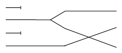
Figure 14. Right inverse functional form.

Let $f\colon\underline{3}\to\underline{4}$ s.t. $f(0)=f(2)=1$ and $f(1)=3$. Then, $\mathrm{riff}_{f}:(4,3)$ can be defined as follows (see Fig. 14):

$$\mathrm{riff}_{f}=(\boldsymbol{\bot}\otimes\ \mathsf{I}\ \otimes\boldsymbol{\bot}\otimes\ \mathsf{I});(\mathsf{\Delta}\otimes\mathsf{I});(\mathsf{I}\ \otimes\mathsf{X})$$

The term $(\boldsymbol{\bot}\otimes\ \mathsf{I}\ \otimes\boldsymbol{\bot}\otimes\ \mathsf{I})$ captures the fact that $0$ and $2$ are not in the image of $f$ (i.e., we write $\boldsymbol{\bot}$ attached to the corresponding ports), while $1$ and $3$ are (i.e., we write $\mathsf{I}$ for those ports). Term $(\mathsf{\Delta}\otimes\ \mathsf{I})$ says that the pre-image of $1$ has two elements (i.e., $\mathsf{\Delta}$) while the pre-image of $3$ has 1(i.e., $\mathsf{I}$). Finally, term $(\mathsf{I}\ \otimes\mathsf{X})$ sorts the connections to the proper ports.

Lemma 33 ensures that the only transitions of $\mathrm{riff}_{f}$ under the strong semantics are those in which $U\subseteq\underline{4}$ is observed over the left interface while its pre-image is observed over the right interface. For instance, $\mathrm{riff}_{f}\raise 1.0pt\hbox{$\;\mathrel{\mathop{\mathchoice{\leavevmode\vtop{\halign{\hfil$\displaystyle#$\hfil\cr\scriptstyle\xrightarrow{\,1010\,}\cr{\lower 1.99997pt\hbox{$\scriptstyle{}_{000}$}}\crcr}}}{\leavevmode\vtop{\halign{\hfil$\textstyle#$\hfil\cr\scriptstyle\xrightarrow{\,1010\,}\cr{\lower 1.99997pt\hbox{$\scriptstyle{}_{000}$}}\crcr}}}{\leavevmode\vtop{\halign{\hfil$\scriptstyle#$\hfil\cr\scriptstyle\xrightarrow{\,1010\,}\cr{\lower 1.39998pt\hbox{$\scriptstyle{}_{000}$}}\crcr}}}{\leavevmode\vtop{\halign{\hfil$\scriptscriptstyle#$\hfil\cr\scriptstyle\xrightarrow{\,1010\,}\cr{\lower 0.99998pt\hbox{$\scriptstyle{}_{000}$}}\crcr}}}}}\;$}\mathrm{riff}_{f}$ (i.e., $f^{-1}(\{0,2\})=\varnothing$), $\mathrm{riff}_{f}\raise 1.0pt\hbox{$\;\mathrel{\mathop{\mathchoice{\leavevmode\vtop{\halign{\hfil$\displaystyle#$\hfil\cr\scriptstyle\xrightarrow{\,0100\,}\cr{\lower 1.99997pt\hbox{$\scriptstyle{}_{101}$}}\crcr}}}{\leavevmode\vtop{\halign{\hfil$\textstyle#$\hfil\cr\scriptstyle\xrightarrow{\,0100\,}\cr{\lower 1.99997pt\hbox{$\scriptstyle{}_{101}$}}\crcr}}}{\leavevmode\vtop{\halign{\hfil$\scriptstyle#$\hfil\cr\scriptstyle\xrightarrow{\,0100\,}\cr{\lower 1.39998pt\hbox{$\scriptstyle{}_{101}$}}\crcr}}}{\leavevmode\vtop{\halign{\hfil$\scriptscriptstyle#$\hfil\cr\scriptstyle\xrightarrow{\,0100\,}\cr{\lower 0.99998pt\hbox{$\scriptstyle{}_{101}$}}\crcr}}}}}\;$}\mathrm{riff}_{f}$ (i.e., $f^{-1}(\{1\})=\{0,2\}$), $\mathrm{riff}_{f}\raise 1.0pt\hbox{$\;\mathrel{\mathop{\mathchoice{\leavevmode\vtop{\halign{\hfil$\displaystyle#$\hfil\cr\scriptstyle\xrightarrow{\,1101\,}\cr{\lower 1.99997pt\hbox{$\scriptstyle{}_{111}$}}\crcr}}}{\leavevmode\vtop{\halign{\hfil$\textstyle#$\hfil\cr\scriptstyle\xrightarrow{\,1101\,}\cr{\lower 1.99997pt\hbox{$\scriptstyle{}_{111}$}}\crcr}}}{\leavevmode\vtop{\halign{\hfil$\scriptstyle#$\hfil\cr\scriptstyle\xrightarrow{\,1101\,}\cr{\lower 1.39998pt\hbox{$\scriptstyle{}_{111}$}}\crcr}}}{\leavevmode\vtop{\halign{\hfil$\scriptscriptstyle#$\hfil\cr\scriptstyle\xrightarrow{\,1101\,}\cr{\lower 0.99998pt\hbox{$\scriptstyle{}_{111}$}}\crcr}}}}}\;$}\mathrm{riff}_{f}$ (i.e., $f^{-1}(\{0,1,3\})=\{0,1,2\}$), and $\mathrm{riff}_{f}\raise 1.0pt\hbox{$\;\mathrel{\mathop{\mathchoice{\leavevmode\vtop{\halign{\hfil$\displaystyle#$\hfil\cr\scriptstyle\xrightarrow{\,0000\,}\cr{\lower 1.99997pt\hbox{$\scriptstyle{}_{000}$}}\crcr}}}{\leavevmode\vtop{\halign{\hfil$\textstyle#$\hfil\cr\scriptstyle\xrightarrow{\,0000\,}\cr{\lower 1.99997pt\hbox{$\scriptstyle{}_{000}$}}\crcr}}}{\leavevmode\vtop{\halign{\hfil$\scriptstyle#$\hfil\cr\scriptstyle\xrightarrow{\,0000\,}\cr{\lower 1.39998pt\hbox{$\scriptstyle{}_{000}$}}\crcr}}}{\leavevmode\vtop{\halign{\hfil$\scriptscriptstyle#$\hfil\cr\scriptstyle\xrightarrow{\,0000\,}\cr{\lower 0.99998pt\hbox{$\scriptstyle{}_{000}$}}\crcr}}}}}\;$}\mathrm{riff}_{f}$ (i.e., $f^{-1}(\varnothing)=\varnothing$) among others. Similarly, for the weak semantics we can obtain, e.g., $\mathrm{riff}_{f}\xLongrightarrow[212]{2201}\mathrm{riff}_{f}$ (i.e., $f^{-1}(\{0,0,1,1,3\})=\{0,0,1,2,2\}$). The term $\mathrm{liff}_{f}:(3,4)$ can be defined analogously by “mirroring” $\mathrm{riff}_{f}:(4,3)$, i.e.,

$$\mathrm{liff}_{f}=(\mathsf{I}\ \otimes\mathsf{X});(\mathchoice{{\rotatebox[origin={c}]{180.0}{$\mathsf{\Delta}$}}\displaystyle}{{\rotatebox[origin={c}]{180.0}{$\mathsf{\Delta}$}}\textstyle}{\!{\rotatebox[origin={c}]{180.0}{$\scriptstyle\mathsf{\Delta}$}}\!\scriptstyle}{{\rotatebox[origin={c}]{180.0}{$\scriptscriptstyle\mathsf{\Delta}$}}\scriptscriptstyle}\otimes\ \mathsf{I});(\boldsymbol{\top}\otimes\ \mathsf{I}\ \otimes\boldsymbol{\top}\otimes\ \mathsf{I}).$$

[Direct functional form] A term $t\mathrel{:}(k,\,l)$ is said to be in right direct functional form when it is in $T_{\{\mathsf{X}\}}\mathrel{;}T_{\{\mathsf{V}\}}\mathrel{;}T_{\{\,\boldsymbol{\uparrow}\,\}}$ Dually, $t\mathrel{:}(k,\,l)$ is in left direct functional form when it is in $T_{\{\,\boldsymbol{\downarrow}\,\}}\mathrel{;}T_{\{\mathsf{\Lambda}\}}\mathrel{;}T_{\{\mathsf{X}\}}$

Lemma 34.

For each function $f\colon\underline{k}\to\underline{l}$ there exists a term $\mathrm{rdff}_{f}\mathrel{:}(k,\,l)$ in right direct functional form, the dynamics of which are characterised by the following:

$$\mathrm{rdff}_{f}\raise 1.0pt\hbox{$\;\mathrel{\mathop{\mathchoice{\leavevmode\vtop{\halign{\hfil$\displaystyle#$\hfil\cr\scriptstyle\xrightarrow{\,\alpha\,}\cr{\lower 1.99997pt\hbox{$\scriptstyle{}_{\beta}$}}\crcr}}}{\leavevmode\vtop{\halign{\hfil$\textstyle#$\hfil\cr\scriptstyle\xrightarrow{\,\alpha\,}\cr{\lower 1.99997pt\hbox{$\scriptstyle{}_{\beta}$}}\crcr}}}{\leavevmode\vtop{\halign{\hfil$\scriptstyle#$\hfil\cr\scriptstyle\xrightarrow{\,\alpha\,}\cr{\lower 1.39998pt\hbox{$\scriptstyle{}_{\beta}$}}\crcr}}}{\leavevmode\vtop{\halign{\hfil$\scriptscriptstyle#$\hfil\cr\scriptstyle\xrightarrow{\,\alpha\,}\cr{\lower 0.99998pt\hbox{$\scriptstyle{}_{\beta}$}}\crcr}}}}}\;$}\mathrm{rdff}_{f}\ \Leftrightarrow\ \exists U\subseteq\underline{k}\mbox{ s.t. }\forall u,v\in U.\;u\neq v\Rightarrow f(u)\neq f(v),\,\alpha={\ulcorner U\urcorner}\mbox{ and }\beta={\ulcorner f(U)\urcorner}$$

$$\mathrm{rdff}_{f}\raise 1.0pt\hbox{$\;\mathrel{\mathop{\mathchoice{\leavevmode\vtop{\halign{\hfil$\displaystyle#$\hfil\cr\scriptstyle\Longrightarrow\cr{\lower-6.00006pt\hbox{$\scriptstyle{}_{\alpha}$}}\cr{\lower 3.00003pt\hbox{$\scriptstyle{}_{\beta}$}}\crcr}}}{\leavevmode\vtop{\halign{\hfil$\textstyle#$\hfil\cr\scriptstyle\Longrightarrow\cr{\lower-6.00006pt\hbox{$\scriptstyle{}_{\alpha}$}}\cr{\lower 3.00003pt\hbox{$\scriptstyle{}_{\beta}$}}\crcr}}}{\leavevmode\vtop{\halign{\hfil$\scriptstyle#$\hfil\cr\scriptstyle\Longrightarrow\cr{\lower-4.20004pt\hbox{$\scriptstyle{}_{\alpha}$}}\cr{\lower 2.10002pt\hbox{$\scriptstyle{}_{\beta}$}}\crcr}}}{\leavevmode\vtop{\halign{\hfil$\scriptscriptstyle#$\hfil\cr\scriptstyle\Longrightarrow\cr{\lower-3.00003pt\hbox{$\scriptstyle{}_{\alpha}$}}\cr{\lower 1.50002pt\hbox{$\scriptstyle{}_{\beta}$}}\crcr}}}}}\;$}\mathrm{rdff}_{f}\ \Leftrightarrow\ \exists\mathcal{U}\in\mathcal{M}_{\underline{k}}\mbox{ s.t. }\alpha={\ulcorner\mathcal{U}\urcorner}\mbox{ and }\beta={\ulcorner f(\mathcal{U})\urcorner}$$

The symmetric result holds for terms $t\mathrel{:}(l,\,k)$ in left direct functional form. That is, there exists a term $\mathrm{ldff}_{f}\mathrel{:}(l,\,k)$ in left direct functional form with semantics characterised by the following:

$$\mathrm{ldff}_{f}\raise 1.0pt\hbox{$\;\mathrel{\mathop{\mathchoice{\leavevmode\vtop{\halign{\hfil$\displaystyle#$\hfil\cr\scriptstyle\xrightarrow{\,\alpha\,}\cr{\lower 1.99997pt\hbox{$\scriptstyle{}_{\beta}$}}\crcr}}}{\leavevmode\vtop{\halign{\hfil$\textstyle#$\hfil\cr\scriptstyle\xrightarrow{\,\alpha\,}\cr{\lower 1.99997pt\hbox{$\scriptstyle{}_{\beta}$}}\crcr}}}{\leavevmode\vtop{\halign{\hfil$\scriptstyle#$\hfil\cr\scriptstyle\xrightarrow{\,\alpha\,}\cr{\lower 1.39998pt\hbox{$\scriptstyle{}_{\beta}$}}\crcr}}}{\leavevmode\vtop{\halign{\hfil$\scriptscriptstyle#$\hfil\cr\scriptstyle\xrightarrow{\,\alpha\,}\cr{\lower 0.99998pt\hbox{$\scriptstyle{}_{\beta}$}}\crcr}}}}}\;$}\mathrm{ldff}_{f}\ \Leftrightarrow\ \exists U\subseteq\underline{k}\mbox{ s.t. }\forall u,v\in U.\;u\neq v\Rightarrow f(u)\neq f(v),\,\beta={\ulcorner U\urcorner}\mbox{ and }\alpha={\ulcorner f(U)\urcorner}$$

$$\mathrm{ldff}_{f}\raise 1.0pt\hbox{$\;\mathrel{\mathop{\mathchoice{\leavevmode\vtop{\halign{\hfil$\displaystyle#$\hfil\cr\scriptstyle\Longrightarrow\cr{\lower-6.00006pt\hbox{$\scriptstyle{}_{\alpha}$}}\cr{\lower 3.00003pt\hbox{$\scriptstyle{}_{\beta}$}}\crcr}}}{\leavevmode\vtop{\halign{\hfil$\textstyle#$\hfil\cr\scriptstyle\Longrightarrow\cr{\lower-6.00006pt\hbox{$\scriptstyle{}_{\alpha}$}}\cr{\lower 3.00003pt\hbox{$\scriptstyle{}_{\beta}$}}\crcr}}}{\leavevmode\vtop{\halign{\hfil$\scriptstyle#$\hfil\cr\scriptstyle\Longrightarrow\cr{\lower-4.20004pt\hbox{$\scriptstyle{}_{\alpha}$}}\cr{\lower 2.10002pt\hbox{$\scriptstyle{}_{\beta}$}}\crcr}}}{\leavevmode\vtop{\halign{\hfil$\scriptscriptstyle#$\hfil\cr\scriptstyle\Longrightarrow\cr{\lower-3.00003pt\hbox{$\scriptstyle{}_{\alpha}$}}\cr{\lower 1.50002pt\hbox{$\scriptstyle{}_{\beta}$}}\crcr}}}}}\;$}\mathrm{ldff}_{f}\ \Leftrightarrow\ \exists\mathcal{U}\in\mathcal{M}_{\underline{k}}\mbox{ s.t. }\beta={\ulcorner\mathcal{U}\urcorner}\mbox{ and }\alpha={\ulcorner f(\mathcal{U})\urcorner}.$$

Proof 9.2.

In Appendix D.

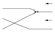
Figure 15. Right direct functional form.

The right direct functional form for $f$ introduced in Example 9.1 is as follow (see Fig. 15):

$$\mathrm{rdff}_{f}=(\mathsf{I}\otimes\mathsf{X});(\mathsf{V}\otimes\mathsf{I});(\,\boldsymbol{\downarrow}\,\otimes\ \mathsf{I}\ \otimes\,\boldsymbol{\downarrow}\,\otimes\ \mathsf{I}).$$

The construction is analogous to the inverse functional form in Example 9.1. The term $(\mathsf{I}\otimes\mathsf{X})$ exchange the order of wires appropriately (it switches the ports $1$ and $2$), then the term $(\mathsf{V}\otimes\mathsf{I})$ states the values $0$ and $2$ are mutually exclusive because they have the same image (i.e., $f(0)=f(2)=1$). Finally, $\,\boldsymbol{\downarrow}\,$ in $(\,\boldsymbol{\downarrow}\,\otimes\ \mathsf{I}\ \otimes\,\boldsymbol{\downarrow}\,\otimes\ \mathsf{I})$ denotes that $0$ and $2$ (over the right interface) are not part of the image of $f$. It is worth noticing that the following transitions $\mathrm{rdff}_{f}\raise 1.0pt\hbox{$\;\mathrel{\mathop{\mathchoice{\leavevmode\vtop{\halign{\hfil$\displaystyle#$\hfil\cr\scriptstyle\xrightarrow{\,100\,}\cr{\lower 1.99997pt\hbox{$\scriptstyle{}_{0100}$}}\crcr}}}{\leavevmode\vtop{\halign{\hfil$\textstyle#$\hfil\cr\scriptstyle\xrightarrow{\,100\,}\cr{\lower 1.99997pt\hbox{$\scriptstyle{}_{0100}$}}\crcr}}}{\leavevmode\vtop{\halign{\hfil$\scriptstyle#$\hfil\cr\scriptstyle\xrightarrow{\,100\,}\cr{\lower 1.39998pt\hbox{$\scriptstyle{}_{0100}$}}\crcr}}}{\leavevmode\vtop{\halign{\hfil$\scriptscriptstyle#$\hfil\cr\scriptstyle\xrightarrow{\,100\,}\cr{\lower 0.99998pt\hbox{$\scriptstyle{}_{0100}$}}\crcr}}}}}\;$}\mathrm{rdff}_{f}$ (i.e., $f(\{0\})=\{1\}$), $\mathrm{rdff}_{f}\raise 1.0pt\hbox{$\;\mathrel{\mathop{\mathchoice{\leavevmode\vtop{\halign{\hfil$\displaystyle#$\hfil\cr\scriptstyle\xrightarrow{\,001\,}\cr{\lower 1.99997pt\hbox{$\scriptstyle{}_{0100}$}}\crcr}}}{\leavevmode\vtop{\halign{\hfil$\textstyle#$\hfil\cr\scriptstyle\xrightarrow{\,001\,}\cr{\lower 1.99997pt\hbox{$\scriptstyle{}_{0100}$}}\crcr}}}{\leavevmode\vtop{\halign{\hfil$\scriptstyle#$\hfil\cr\scriptstyle\xrightarrow{\,001\,}\cr{\lower 1.39998pt\hbox{$\scriptstyle{}_{0100}$}}\crcr}}}{\leavevmode\vtop{\halign{\hfil$\scriptscriptstyle#$\hfil\cr\scriptstyle\xrightarrow{\,001\,}\cr{\lower 0.99998pt\hbox{$\scriptstyle{}_{0100}$}}\crcr}}}}}\;$}\mathrm{rdff}_{f}$ (i.e., $f(\{2\})=\{1\}$) and $\mathrm{rdff}_{f}\raise 1.0pt\hbox{$\;\mathrel{\mathop{\mathchoice{\leavevmode\vtop{\halign{\hfil$\displaystyle#$\hfil\cr\scriptstyle\xrightarrow{\,011\,}\cr{\lower 1.99997pt\hbox{$\scriptstyle{}_{0101}$}}\crcr}}}{\leavevmode\vtop{\halign{\hfil$\textstyle#$\hfil\cr\scriptstyle\xrightarrow{\,011\,}\cr{\lower 1.99997pt\hbox{$\scriptstyle{}_{0101}$}}\crcr}}}{\leavevmode\vtop{\halign{\hfil$\scriptstyle#$\hfil\cr\scriptstyle\xrightarrow{\,011\,}\cr{\lower 1.39998pt\hbox{$\scriptstyle{}_{0101}$}}\crcr}}}{\leavevmode\vtop{\halign{\hfil$\scriptscriptstyle#$\hfil\cr\scriptstyle\xrightarrow{\,011\,}\cr{\lower 0.99998pt\hbox{$\scriptstyle{}_{0101}$}}\crcr}}}}}\;$}\mathrm{rdff}_{f}$ (i.e., $f(\{1,2\})=\{1,3\}$) are derivable under the strong semantics, while the transition $\mathrm{rdff}_{f}\raise 1.0pt\hbox{$\;\mathrel{\mathop{\mathchoice{\leavevmode\vtop{\halign{\hfil$\displaystyle#$\hfil\cr\scriptstyle\xrightarrow{\,101\,}\cr{\lower 1.99997pt\hbox{$\scriptstyle{}_{0100}$}}\crcr}}}{\leavevmode\vtop{\halign{\hfil$\textstyle#$\hfil\cr\scriptstyle\xrightarrow{\,101\,}\cr{\lower 1.99997pt\hbox{$\scriptstyle{}_{0100}$}}\crcr}}}{\leavevmode\vtop{\halign{\hfil$\scriptstyle#$\hfil\cr\scriptstyle\xrightarrow{\,101\,}\cr{\lower 1.39998pt\hbox{$\scriptstyle{}_{0100}$}}\crcr}}}{\leavevmode\vtop{\halign{\hfil$\scriptscriptstyle#$\hfil\cr\scriptstyle\xrightarrow{\,101\,}\cr{\lower 0.99998pt\hbox{$\scriptstyle{}_{0100}$}}\crcr}}}}}\;$}\mathrm{rdff}_{f}$ (i.e., $f(\{0,2\})=\{1\}$) cannot be derived because the domain values $0$ and $2$ has the same image and, thus, are in mutual exclusion. Differently, the weak semantics allows us to consider multisets of domain values that may have the same image, e.g., we can derive $\mathrm{rdff}_{f}\xLongrightarrow[0200]{101}\mathrm{rdff}_{f}$ (i.e., $f(\{0,2\})=\{1,1\}$).

Similarly, we can define the left direct functional form of $f$ as below:

$$\mathrm{ldff}_{f}=(\,\boldsymbol{\downarrow}\,\otimes\ \mathsf{I}\ \otimes\,\boldsymbol{\downarrow}\,\otimes\ \mathsf{I});(\mathsf{\Lambda}\otimes\mathsf{I});(\mathsf{I}\otimes\mathsf{X}).$$

The dynamics of $\mathrm{ldff}_{f}$ can be interpreted analogously to $\mathrm{rdff}_{f}$, after swapping the interfaces.

9.2. Relational forms

We now identify two classes of terms of the Petri calculus: the left and right relational forms. These will be used in the translation from C/E nets to Petri calculus terms with strong semantics for representing the functions ${}^{\circ}\_,\_^{\circ},{}^{\bullet}\_,\_^{\bullet}$.

A term $t\mathrel{:}(k,\,l)$ is in right relational form when it is in

$$T_{\{\boldsymbol{\bot}\}}\mathrel{;}T_{\{\mathsf{\Delta}\}}\mathrel{;}T_{\{\mathsf{X}\}}\mathrel{;}T_{\{\mathsf{V}\}}\mathrel{;}T_{\{\,\boldsymbol{\uparrow}\,\}}.$$

Dually, $t$ is said to be in left relational form when it is in

$$T_{\{\,\boldsymbol{\downarrow}\,\}}\mathrel{;}T_{\{\mathsf{\Lambda}\}}\mathrel{;}T_{\{\mathsf{X}\}}\mathrel{;}T_{\{\mathchoice{{\rotatebox[origin={c}]{180.0}{$\mathsf{\Delta}$}}\displaystyle}{{\rotatebox[origin={c}]{180.0}{$\mathsf{\Delta}$}}\textstyle}{\!{\rotatebox[origin={c}]{180.0}{$\scriptstyle\mathsf{\Delta}$}}\!\scriptstyle}{{\rotatebox[origin={c}]{180.0}{$\scriptscriptstyle\mathsf{\Delta}$}}\scriptscriptstyle}\}}\mathrel{;}T_{\{\boldsymbol{\top}\}}.$$

The following result spells out the significance of the relational forms.

Lemma 35.

For each function $f\colon\underline{k}\to 2^{\underline{l}}$ there exists a term $\rho_{f}\mathrel{:}(k,\,l)$ in right relational form, the dynamics of which are characterised by the following:

$$\rho_{f}\raise 1.0pt\hbox{$\;\mathrel{\mathop{\mathchoice{\leavevmode\vtop{\halign{\hfil$\displaystyle#$\hfil\cr\scriptstyle\xrightarrow{\,\alpha\,}\cr{\lower 1.99997pt\hbox{$\scriptstyle{}_{\beta}$}}\crcr}}}{\leavevmode\vtop{\halign{\hfil$\textstyle#$\hfil\cr\scriptstyle\xrightarrow{\,\alpha\,}\cr{\lower 1.99997pt\hbox{$\scriptstyle{}_{\beta}$}}\crcr}}}{\leavevmode\vtop{\halign{\hfil$\scriptstyle#$\hfil\cr\scriptstyle\xrightarrow{\,\alpha\,}\cr{\lower 1.39998pt\hbox{$\scriptstyle{}_{\beta}$}}\crcr}}}{\leavevmode\vtop{\halign{\hfil$\scriptscriptstyle#$\hfil\cr\scriptstyle\xrightarrow{\,\alpha\,}\cr{\lower 0.99998pt\hbox{$\scriptstyle{}_{\beta}$}}\crcr}}}}}\;$}\rho_{f}\ \Leftrightarrow\ \exists U\subseteq\underline{k}\mbox{ s.t. }\forall u,v\in U.\;u\neq v\Rightarrow f(u)\mathrel{\cap}f(v)=\varnothing,\,\alpha={\ulcorner U\urcorner}\mbox{ and }\beta={\ulcorner f(U)\urcorner}$$

The symmetric result holds for functions $f\colon\underline{k}\to 2^{\underline{l}}$ and terms $t\mathrel{:}(l,\,k)$ in left relational form. That is, there exists $\lambda_{f}\mathrel{:}(l,\,k)$ in left relational form with semantics

$$\lambda_{f}\raise 1.0pt\hbox{$\;\mathrel{\mathop{\mathchoice{\leavevmode\vtop{\halign{\hfil$\displaystyle#$\hfil\cr\scriptstyle\xrightarrow{\,\alpha\,}\cr{\lower 1.99997pt\hbox{$\scriptstyle{}_{\beta}$}}\crcr}}}{\leavevmode\vtop{\halign{\hfil$\textstyle#$\hfil\cr\scriptstyle\xrightarrow{\,\alpha\,}\cr{\lower 1.99997pt\hbox{$\scriptstyle{}_{\beta}$}}\crcr}}}{\leavevmode\vtop{\halign{\hfil$\scriptstyle#$\hfil\cr\scriptstyle\xrightarrow{\,\alpha\,}\cr{\lower 1.39998pt\hbox{$\scriptstyle{}_{\beta}$}}\crcr}}}{\leavevmode\vtop{\halign{\hfil$\scriptscriptstyle#$\hfil\cr\scriptstyle\xrightarrow{\,\alpha\,}\cr{\lower 0.99998pt\hbox{$\scriptstyle{}_{\beta}$}}\crcr}}}}}\;$}\lambda_{f}\ \Leftrightarrow\ \exists U\subseteq\underline{k}\mbox{ s.t. }\forall u,v\in U.\;u\neq v\Rightarrow f(u)\mathrel{\cap}f(v)=\varnothing,\,\beta={\ulcorner U\urcorner}\mbox{ and }\alpha={\ulcorner f(U)\urcorner}$$

Proof 9.3.

To give a function $f:\underline{k}\to 2^{\underline{l}}$ is to give functions $f_{l}:\underline{m}\to\underline{k}$, $f_{r}:\underline{m}\to\underline{l}$ such that $(f_{l},f_{r}):\underline{m}\to\underline{k}\times\underline{l}$ is injective and for any $i<k$, $f(i)=f_{r}(f_{l}^{-1}(i))$. Let

$$\rho_{f}\stackrel{{\scriptstyle\mathrm{def}}}{{=}}\mathrm{riff}_{f_{l}}\mathrel{;}\mathrm{rdff}_{f_{r}}\mbox{ and }\lambda_{f}\stackrel{{\scriptstyle\mathrm{def}}}{{=}}\mathrm{ldff}_{f_{r}}\mathrel{;}\mathrm{liff}_{f_{l}}.$$

Then the required characterisations follow directly from the characterisations of inverse and direct functional forms given in Lemmas 33 and 34.

(a) $\mathrm{riff}_{f_{l}}$.

(b) $\mathrm{rdff}_{f_{r}}$.

(c) $\rho_{f}$.

Figure 16. Right relational form.

Let $f\colon\underline{4}\to 2^{\underline{4}}$ defined by $f(0),f(1)=\{0\}$, $f(2)=\varnothing$ and $f(3)=\{1,2\}$. Figure 16(c) shows the right relational form $\rho_{f}$ of $f$ that can be obtained, as suggested by proof of Lemma 35, from the combination of the functions $f_{l}\colon\underline{4}\to\underline{4}$ and $f_{r}\colon\underline{4}\to\underline{4}$ defined by $f_{l}(0)=0$, $f_{l}(1)=1$, $f_{l}(2)=f_{l}(3)=3$, $f_{r}(0)=f_{r}(1)=0$, $f_{r}(2)=1$ and $f_{r}(3)=2$ (the corresponding $\mathrm{riff}_{f_{l}}$ and $\mathrm{rdff}_{f_{r}}$ are in Fig. 16(a) and 16(b), respectively).

Assume now that $f$ above is the postset function of a C/E net consisting on four transitions (named $0,1,2,3$) and four places (also named $0,1,2,3$). Intuitively, the term $\rho_{f}$ accounts for the tokens produced during the execution of a step. The left interface stands for transitions while the right interface stands for places. For instance, the transition $\mathrm{\rho}_{f}\xLongrightarrow[1110]{1011}\mathrm{\rho}_{f}$ (i.e., $f(\{0,2,3\})=\{0,1,2\}$) stands for tokens produced by the simultaneous firing of the transitions $0$, $2$, and $3$ in the places $0$, $1$ and $2$. Note that transitions $0$ and $1$ are not independent and, hence, they cannot be fired simultaneously. This fact is made evident in $\rho_{f}$ because the ports $0$ and $1$ over the left interface are in mutual exclusion.

The left relational form $\lambda_{f}$ can be defined analogously. Dually, $\lambda_{f}$ can be interpreted as a term describing the consumption of tokens during the execution of several mutually independent transitions.

Note that not all terms $t\mathrel{:}(k,\,l)$ in right relational form have the behaviour of $\rho_{f}$ for some $f\colon\underline{k}\to 2^{\underline{l}}$; a simple counterexample is $\mathsf{\Delta}\mathrel{;}\mathsf{V}\mathrel{:}(1,\,1)$ whose only reduction under the strong semantics is $\mathsf{\Delta}\mathrel{;}\mathsf{V}\raise 1.0pt\hbox{$\;\mathrel{\mathop{\mathchoice{\leavevmode\vtop{\halign{\hfil$\displaystyle#$\hfil\cr\scriptstyle\xrightarrow{\,0\,}\cr{\lower 1.99997pt\hbox{$\scriptstyle{}_{0}$}}\crcr}}}{\leavevmode\vtop{\halign{\hfil$\textstyle#$\hfil\cr\scriptstyle\xrightarrow{\,0\,}\cr{\lower 1.99997pt\hbox{$\scriptstyle{}_{0}$}}\crcr}}}{\leavevmode\vtop{\halign{\hfil$\scriptstyle#$\hfil\cr\scriptstyle\xrightarrow{\,0\,}\cr{\lower 1.39998pt\hbox{$\scriptstyle{}_{0}$}}\crcr}}}{\leavevmode\vtop{\halign{\hfil$\scriptscriptstyle#$\hfil\cr\scriptstyle\xrightarrow{\,0\,}\cr{\lower 0.99998pt\hbox{$\scriptstyle{}_{0}$}}\crcr}}}}}\;$}\mathsf{\Delta}\mathrel{;}\mathsf{V}$.

9.3. Contention

Recall that contention is an irreflexive, symmetric relation on transitions, that restricts the sets of transitions that can be fired together.

Now consider the term $c$, defined below.

$$c\stackrel{{\scriptstyle\mathrm{def}}}{{=}}(\mathsf{\Delta}\otimes\mathsf{\Delta})\mathrel{;}(\mathsf{I}\otimes\mathsf{X}\otimes\mathsf{I})\mathrel{;}(\mathsf{I}\otimes\mathsf{I}\otimes(\mathsf{V}\mathrel{;}\boldsymbol{\bot})).$$

It is not difficult to verify that $c$ has its behaviour characterised by the following transitions:

$$c\raise 1.0pt\hbox{$\;\mathrel{\mathop{\mathchoice{\leavevmode\vtop{\halign{\hfil$\displaystyle#$\hfil\cr\scriptstyle\xrightarrow{\,00\,}\cr{\lower 1.99997pt\hbox{$\scriptstyle{}_{00}$}}\crcr}}}{\leavevmode\vtop{\halign{\hfil$\textstyle#$\hfil\cr\scriptstyle\xrightarrow{\,00\,}\cr{\lower 1.99997pt\hbox{$\scriptstyle{}_{00}$}}\crcr}}}{\leavevmode\vtop{\halign{\hfil$\scriptstyle#$\hfil\cr\scriptstyle\xrightarrow{\,00\,}\cr{\lower 1.39998pt\hbox{$\scriptstyle{}_{00}$}}\crcr}}}{\leavevmode\vtop{\halign{\hfil$\scriptscriptstyle#$\hfil\cr\scriptstyle\xrightarrow{\,00\,}\cr{\lower 0.99998pt\hbox{$\scriptstyle{}_{00}$}}\crcr}}}}}\;$}c,\quad c\raise 1.0pt\hbox{$\;\mathrel{\mathop{\mathchoice{\leavevmode\vtop{\halign{\hfil$\displaystyle#$\hfil\cr\scriptstyle\xrightarrow{\,10\,}\cr{\lower 1.99997pt\hbox{$\scriptstyle{}_{10}$}}\crcr}}}{\leavevmode\vtop{\halign{\hfil$\textstyle#$\hfil\cr\scriptstyle\xrightarrow{\,10\,}\cr{\lower 1.99997pt\hbox{$\scriptstyle{}_{10}$}}\crcr}}}{\leavevmode\vtop{\halign{\hfil$\scriptstyle#$\hfil\cr\scriptstyle\xrightarrow{\,10\,}\cr{\lower 1.39998pt\hbox{$\scriptstyle{}_{10}$}}\crcr}}}{\leavevmode\vtop{\halign{\hfil$\scriptscriptstyle#$\hfil\cr\scriptstyle\xrightarrow{\,10\,}\cr{\lower 0.99998pt\hbox{$\scriptstyle{}_{10}$}}\crcr}}}}}\;$}c,\quad c\raise 1.0pt\hbox{$\;\mathrel{\mathop{\mathchoice{\leavevmode\vtop{\halign{\hfil$\displaystyle#$\hfil\cr\scriptstyle\xrightarrow{\,01\,}\cr{\lower 1.99997pt\hbox{$\scriptstyle{}_{01}$}}\crcr}}}{\leavevmode\vtop{\halign{\hfil$\textstyle#$\hfil\cr\scriptstyle\xrightarrow{\,01\,}\cr{\lower 1.99997pt\hbox{$\scriptstyle{}_{01}$}}\crcr}}}{\leavevmode\vtop{\halign{\hfil$\scriptstyle#$\hfil\cr\scriptstyle\xrightarrow{\,01\,}\cr{\lower 1.39998pt\hbox{$\scriptstyle{}_{01}$}}\crcr}}}{\leavevmode\vtop{\halign{\hfil$\scriptscriptstyle#$\hfil\cr\scriptstyle\xrightarrow{\,01\,}\cr{\lower 0.99998pt\hbox{$\scriptstyle{}_{01}$}}\crcr}}}}}\;$}c.$$

Given a set of transitions $\underline{t}$ and a contention relation $\#\subseteq\underline{t}\times\underline{t}$, here we will define a term $\#_{t}:\underline{t}\to\underline{t}$ with semantics:

$${\#}_{t}\raise 1.0pt\hbox{$\;\mathrel{\mathop{\mathchoice{\leavevmode\vtop{\halign{\hfil$\displaystyle#$\hfil\cr\scriptstyle\xrightarrow{\,{\ulcorner U\urcorner}\,}\cr{\lower 1.99997pt\hbox{$\scriptstyle{}_{{\ulcorner V\urcorner}}$}}\crcr}}}{\leavevmode\vtop{\halign{\hfil$\textstyle#$\hfil\cr\scriptstyle\xrightarrow{\,{\ulcorner U\urcorner}\,}\cr{\lower 1.99997pt\hbox{$\scriptstyle{}_{{\ulcorner V\urcorner}}$}}\crcr}}}{\leavevmode\vtop{\halign{\hfil$\scriptstyle#$\hfil\cr\scriptstyle\xrightarrow{\,{\ulcorner U\urcorner}\,}\cr{\lower 1.39998pt\hbox{$\scriptstyle{}_{{\ulcorner V\urcorner}}$}}\crcr}}}{\leavevmode\vtop{\halign{\hfil$\scriptscriptstyle#$\hfil\cr\scriptstyle\xrightarrow{\,{\ulcorner U\urcorner}\,}\cr{\lower 0.99998pt\hbox{$\scriptstyle{}_{{\ulcorner V\urcorner}}$}}\crcr}}}}}\;$}{\#}_{t}\quad\text{iff}\quad U=V\text{ and }\forall u,v\in U.\;\neg(u\#v)$$

We define it by induction on the size of $\#$. The base case is when $\#$ is empty, and in this case we let $\#_{t}=\mathsf{I}_{t}$. Otherwise, there exists $(u,v)\in\#$. Let $\#^{\prime}=\#\backslash\{(u,v),(v,u)\}$. By the inductive hypothesis we have a term ${\#^{\prime}}_{t}:t\to t$ that satisfies the specification wrt the relation $\#^{\prime}$. Now the term ${\#^{\prime}}_{t}\mathrel{;}\mathsf{X}_{u,v}\mathrel{;}\mathsf{I}_{t-2}\otimes c\mathrel{;}\mathsf{X}_{u,v}^{-1}$ has the required behaviour, where $\mathsf{X}_{u,v}$ is a term in $T_{\{\mathsf{X},\mathsf{I}\}}$ that permutes $\underline{t}$, taking $u$ and $v$ to $t-2$ and $t-1$, and $\mathsf{X}_{u,v}^{-1}$ is its inverse.

Figure 17. Circuit diagrammatic representation of the translation from a C/E net to a Petri calculus term.

9.4. Translating C/E nets

Here we present a translation from C/E nets with boundaries, defined in Section 3, to Petri calculus terms as defined in Section 6. Let $N_{X}\colon m\to n=(P,\,T,\,X,\,\#,\,{\rm Phys.~{}Rev.~{}E}{-},\,{-^{\circ}},\,{{}^{\bullet}{-}},\,{{-}^{\bullet}})$ be a finite C/E net with boundary (Definition 2). Assume, without loss of generality, that $P=\underline{p}$ and $T=\underline{t}$ for some $p,t\in\mathbb{N}$. If $p=0$ we let $w_{N_{X}}:(0,0)\stackrel{{\scriptstyle\mathrm{def}}}{{=}}\boldsymbol{\top}\mathrel{;}\boldsymbol{\bot}$, otherwise

$$w_{N_{X}}\mathrel{:}(p,\,p)\ \stackrel{{\scriptstyle\mathrm{def}}}{{=}}\ \bigotimes_{i<p}m_{i}\quad\text{where}\quad m_{i}\stackrel{{\scriptstyle\mathrm{def}}}{{=}}\begin{cases}\mathchoice{\leavevmode\vtop{\halign{\hfil$\displaystyle#$\hfil\cr\bigcirc\cr\bullet\crcr}}}{\leavevmode\vtop{\halign{\hfil$\textstyle#$\hfil\cr\bigcirc\cr\bullet\crcr}}}{\leavevmode\vtop{\halign{\hfil$\scriptstyle#$\hfil\cr\bigcirc\cr\bullet\crcr}}}{\leavevmode\vtop{\halign{\hfil$\scriptscriptstyle#$\hfil\cr\bigcirc\cr\bullet\crcr}}}&\text{if }i\in X\\ \bigcirc&\text{otherwise}\end{cases}$$ (11)

The following technical result will be useful for showing that the encodings of this section are correct.

Lemma 36.

1. $w_{N_{X}}\raise 1.0pt\hbox{$\;\mathrel{\mathop{\mathchoice{\leavevmode\vtop{\halign{\hfil$\displaystyle#$\hfil\cr\scriptstyle\xrightarrow{\,{\ulcorner Z\urcorner}\,}\cr{\lower 1.99997pt\hbox{$\scriptstyle{}_{{\ulcorner W\urcorner}}$}}\crcr}}}{\leavevmode\vtop{\halign{\hfil$\textstyle#$\hfil\cr\scriptstyle\xrightarrow{\,{\ulcorner Z\urcorner}\,}\cr{\lower 1.99997pt\hbox{$\scriptstyle{}_{{\ulcorner W\urcorner}}$}}\crcr}}}{\leavevmode\vtop{\halign{\hfil$\scriptstyle#$\hfil\cr\scriptstyle\xrightarrow{\,{\ulcorner Z\urcorner}\,}\cr{\lower 1.39998pt\hbox{$\scriptstyle{}_{{\ulcorner W\urcorner}}$}}\crcr}}}{\leavevmode\vtop{\halign{\hfil$\scriptscriptstyle#$\hfil\cr\scriptstyle\xrightarrow{\,{\ulcorner Z\urcorner}\,}\cr{\lower 0.99998pt\hbox{$\scriptstyle{}_{{\ulcorner W\urcorner}}$}}\crcr}}}}}\;$}Q$ iff $Q=w_{N_{Y}}$, $W\subseteq X$, $Z\cap X=\varnothing$ and $Y=(X\backslash W)\cup Z$.

2. $w_{N_{X}}\raise 1.0pt\hbox{$\;\mathrel{\mathop{\mathchoice{\leavevmode\vtop{\halign{\hfil$\displaystyle#$\hfil\cr\scriptstyle\Longrightarrow\cr{\lower-6.00006pt\hbox{$\scriptstyle{}_{\alpha}$}}\cr{\lower 3.00003pt\hbox{$\scriptstyle{}_{\beta}$}}\crcr}}}{\leavevmode\vtop{\halign{\hfil$\textstyle#$\hfil\cr\scriptstyle\Longrightarrow\cr{\lower-6.00006pt\hbox{$\scriptstyle{}_{\alpha}$}}\cr{\lower 3.00003pt\hbox{$\scriptstyle{}_{\beta}$}}\crcr}}}{\leavevmode\vtop{\halign{\hfil$\scriptstyle#$\hfil\cr\scriptstyle\Longrightarrow\cr{\lower-4.20004pt\hbox{$\scriptstyle{}_{\alpha}$}}\cr{\lower 2.10002pt\hbox{$\scriptstyle{}_{\beta}$}}\crcr}}}{\leavevmode\vtop{\halign{\hfil$\scriptscriptstyle#$\hfil\cr\scriptstyle\Longrightarrow\cr{\lower-3.00003pt\hbox{$\scriptstyle{}_{\alpha}$}}\cr{\lower 1.50002pt\hbox{$\scriptstyle{}_{\beta}$}}\crcr}}}}}\;$}Q$ iff $Q=w_{N_{Y}}$ and $X+\alpha=Y+\beta$ as multisets.

Proof 9.4.

(i) Examination of either rules ($\boldsymbol{\bot}_{1}$) and ($\boldsymbol{\top}_{1}$), together with the rule (Cut) (when $p=0$) or rules (TkI) and (TkO), together with the rule (Ten) (when $p>0$).

(ii) Combination of (i) with part (ii) of Lemma 20.

The translation of $N$ can now be expressed as:

$$T_{N_{X}}\ \stackrel{{\scriptstyle\mathrm{def}}}{{=}}\ (d_{t}\otimes\lambda_{{{}^{\bullet}{-}}})\mathrel{;}({\#}_{t}\otimes(\mathchoice{{\rotatebox[origin={c}]{180.0}{$\mathsf{\Delta}$}}\displaystyle}{{\rotatebox[origin={c}]{180.0}{$\mathsf{\Delta}$}}\textstyle}{\!{\rotatebox[origin={c}]{180.0}{$\scriptstyle\mathsf{\Delta}$}}\!\scriptstyle}{{\rotatebox[origin={c}]{180.0}{$\scriptscriptstyle\mathsf{\Delta}$}}\scriptscriptstyle}_{t}\mathrel{;}\rho_{{-^{\circ}}}\mathrel{;}w_{N_{X}}\mathrel{;}\lambda_{{\rm Phys.~{}Rev.~{}E}{-}}\mathrel{;}\mathsf{\Delta}_{t}));(e_{t}\otimes\rho_{{{-}^{\bullet}}}).$$ (12)

A schematic circuit diagram representation of the above term is illustrated in Fig. 17, where terms are represented as boxes, sequential composition is the juxtaposition of boxes (to be read from left to right) and parallel composition is shown vertically (read from top to bottom).

The encoding preserves and reflects semantics in a very tight manner, as shown by the following result.

Theorem 37.

Let $N$ be a (finite) C/E net. The following hold:

1. if $N_{X}\raise 1.0pt\hbox{$\;\mathrel{\mathop{\mathchoice{\leavevmode\vtop{\halign{\hfil$\displaystyle#$\hfil\cr\scriptstyle\xrightarrow{\,\alpha\,}\cr{\lower 1.99997pt\hbox{$\scriptstyle{}_{\beta}$}}\crcr}}}{\leavevmode\vtop{\halign{\hfil$\textstyle#$\hfil\cr\scriptstyle\xrightarrow{\,\alpha\,}\cr{\lower 1.99997pt\hbox{$\scriptstyle{}_{\beta}$}}\crcr}}}{\leavevmode\vtop{\halign{\hfil$\scriptstyle#$\hfil\cr\scriptstyle\xrightarrow{\,\alpha\,}\cr{\lower 1.39998pt\hbox{$\scriptstyle{}_{\beta}$}}\crcr}}}{\leavevmode\vtop{\halign{\hfil$\scriptscriptstyle#$\hfil\cr\scriptstyle\xrightarrow{\,\alpha\,}\cr{\lower 0.99998pt\hbox{$\scriptstyle{}_{\beta}$}}\crcr}}}}}\;$}N_{Y}$ then $T_{N_{X}}\raise 1.0pt\hbox{$\;\mathrel{\mathop{\mathchoice{\leavevmode\vtop{\halign{\hfil$\displaystyle#$\hfil\cr\scriptstyle\xrightarrow{\,\alpha\,}\cr{\lower 1.99997pt\hbox{$\scriptstyle{}_{\beta}$}}\crcr}}}{\leavevmode\vtop{\halign{\hfil$\textstyle#$\hfil\cr\scriptstyle\xrightarrow{\,\alpha\,}\cr{\lower 1.99997pt\hbox{$\scriptstyle{}_{\beta}$}}\crcr}}}{\leavevmode\vtop{\halign{\hfil$\scriptstyle#$\hfil\cr\scriptstyle\xrightarrow{\,\alpha\,}\cr{\lower 1.39998pt\hbox{$\scriptstyle{}_{\beta}$}}\crcr}}}{\leavevmode\vtop{\halign{\hfil$\scriptscriptstyle#$\hfil\cr\scriptstyle\xrightarrow{\,\alpha\,}\cr{\lower 0.99998pt\hbox{$\scriptstyle{}_{\beta}$}}\crcr}}}}}\;$}T_{N_{Y}}$;

2. if $T_{N_{X}}\raise 1.0pt\hbox{$\;\mathrel{\mathop{\mathchoice{\leavevmode\vtop{\halign{\hfil$\displaystyle#$\hfil\cr\scriptstyle\xrightarrow{\,\alpha\,}\cr{\lower 1.99997pt\hbox{$\scriptstyle{}_{\beta}$}}\crcr}}}{\leavevmode\vtop{\halign{\hfil$\textstyle#$\hfil\cr\scriptstyle\xrightarrow{\,\alpha\,}\cr{\lower 1.99997pt\hbox{$\scriptstyle{}_{\beta}$}}\crcr}}}{\leavevmode\vtop{\halign{\hfil$\scriptstyle#$\hfil\cr\scriptstyle\xrightarrow{\,\alpha\,}\cr{\lower 1.39998pt\hbox{$\scriptstyle{}_{\beta}$}}\crcr}}}{\leavevmode\vtop{\halign{\hfil$\scriptscriptstyle#$\hfil\cr\scriptstyle\xrightarrow{\,\alpha\,}\cr{\lower 0.99998pt\hbox{$\scriptstyle{}_{\beta}$}}\crcr}}}}}\;$}Q$ then there exists $Y$ such that $Q=T_{N_{Y}}$ and $N_{X}\raise 1.0pt\hbox{$\;\mathrel{\mathop{\mathchoice{\leavevmode\vtop{\halign{\hfil$\displaystyle#$\hfil\cr\scriptstyle\xrightarrow{\,\alpha\,}\cr{\lower 1.99997pt\hbox{$\scriptstyle{}_{\beta}$}}\crcr}}}{\leavevmode\vtop{\halign{\hfil$\textstyle#$\hfil\cr\scriptstyle\xrightarrow{\,\alpha\,}\cr{\lower 1.99997pt\hbox{$\scriptstyle{}_{\beta}$}}\crcr}}}{\leavevmode\vtop{\halign{\hfil$\scriptstyle#$\hfil\cr\scriptstyle\xrightarrow{\,\alpha\,}\cr{\lower 1.39998pt\hbox{$\scriptstyle{}_{\beta}$}}\crcr}}}{\leavevmode\vtop{\halign{\hfil$\scriptscriptstyle#$\hfil\cr\scriptstyle\xrightarrow{\,\alpha\,}\cr{\lower 0.99998pt\hbox{$\scriptstyle{}_{\beta}$}}\crcr}}}}}\;$}N_{Y}$.

Proof 9.5.

In Appendix D.

9.5. Translating P/T nets (and weak C/E nets)

We begin by defining right and left amplifiers $!k,\,k!\mathrel{:}(1,\,1)$ for any $k\in\mathbb{N}$ that will be necessary in order to define multirelational forms, with the latter being needed to translate P/T nets. [Amplifiers] Given $k\in\mathbb{N}_{+}$, the right amplifier $!k\mathrel{:}(1,\,1)$ is defined recursively as follows: $!1\stackrel{{\scriptstyle\mathrm{def}}}{{=}}\mathsf{I}$, $!(k+1)\stackrel{{\scriptstyle\mathrm{def}}}{{=}}\mathsf{\Delta};(!k\otimes\mathsf{I});\mathsf{V}$. Dually, the left amplifier $k!\mathrel{:}(1,\,1)$ is defined: $1!\stackrel{{\scriptstyle\mathrm{def}}}{{=}}\mathsf{I}$, $(k+1)!\stackrel{{\scriptstyle\mathrm{def}}}{{=}}\mathsf{\Lambda};(\mathsf{I}\otimes k!);\mathchoice{{\rotatebox[origin={c}]{180.0}{$\mathsf{\Delta}$}}\displaystyle}{{\rotatebox[origin={c}]{180.0}{$\mathsf{\Delta}$}}\textstyle}{\!{\rotatebox[origin={c}]{180.0}{$\scriptstyle\mathsf{\Delta}$}}\!\scriptstyle}{{\rotatebox[origin={c}]{180.0}{$\scriptscriptstyle\mathsf{\Delta}$}}\scriptscriptstyle}$.

Notice that under the strong semantics of the Petri calculus, for any $k>1$, $k!$ and $!k$ have no non-trivial behaviour (i.e., the only behavior is $k!\raise 1.0pt\hbox{$\;\mathrel{\mathop{\mathchoice{\leavevmode\vtop{\halign{\hfil$\displaystyle#$\hfil\cr\scriptstyle\xrightarrow{\,0\,}\cr{\lower 1.99997pt\hbox{$\scriptstyle{}_{0}$}}\crcr}}}{\leavevmode\vtop{\halign{\hfil$\textstyle#$\hfil\cr\scriptstyle\xrightarrow{\,0\,}\cr{\lower 1.99997pt\hbox{$\scriptstyle{}_{0}$}}\crcr}}}{\leavevmode\vtop{\halign{\hfil$\scriptstyle#$\hfil\cr\scriptstyle\xrightarrow{\,0\,}\cr{\lower 1.39998pt\hbox{$\scriptstyle{}_{0}$}}\crcr}}}{\leavevmode\vtop{\halign{\hfil$\scriptscriptstyle#$\hfil\cr\scriptstyle\xrightarrow{\,0\,}\cr{\lower 0.99998pt\hbox{$\scriptstyle{}_{0}$}}\crcr}}}}}\;$}k!$). Instead, the behaviour of a right amplifier $!k$ under the weak semantics of the Petri calculus, and in both the strong and weak semantics of the P/T calculus, intuitively “amplifies” a signal $k$ times from left to right. Symmetrically, a left amplifier $k!$ amplifies a signal $k$ times from right to left. More formally, their behaviour under the weak semantics of the Petri calculus and both semantics of the P/T calculus is summarised by the following result.

Lemma 38.

Let $a,b\in\mathbb{N}$. Then $!k\raise 1.0pt\hbox{$\;\mathrel{\mathop{\mathchoice{\leavevmode\vtop{\halign{\hfil$\displaystyle#$\hfil\cr\scriptstyle\Longrightarrow\cr{\lower-6.00006pt\hbox{$\scriptstyle{}_{a}$}}\cr{\lower 3.00003pt\hbox{$\scriptstyle{}_{b}$}}\crcr}}}{\leavevmode\vtop{\halign{\hfil$\textstyle#$\hfil\cr\scriptstyle\Longrightarrow\cr{\lower-6.00006pt\hbox{$\scriptstyle{}_{a}$}}\cr{\lower 3.00003pt\hbox{$\scriptstyle{}_{b}$}}\crcr}}}{\leavevmode\vtop{\halign{\hfil$\scriptstyle#$\hfil\cr\scriptstyle\Longrightarrow\cr{\lower-4.20004pt\hbox{$\scriptstyle{}_{a}$}}\cr{\lower 2.10002pt\hbox{$\scriptstyle{}_{b}$}}\crcr}}}{\leavevmode\vtop{\halign{\hfil$\scriptscriptstyle#$\hfil\cr\scriptstyle\Longrightarrow\cr{\lower-3.00003pt\hbox{$\scriptstyle{}_{a}$}}\cr{\lower 1.50002pt\hbox{$\scriptstyle{}_{b}$}}\crcr}}}}}\;$}!k$ iff $b=ka$. Similarly, $k!\raise 1.0pt\hbox{$\;\mathrel{\mathop{\mathchoice{\leavevmode\vtop{\halign{\hfil$\displaystyle#$\hfil\cr\scriptstyle\Longrightarrow\cr{\lower-6.00006pt\hbox{$\scriptstyle{}_{a}$}}\cr{\lower 3.00003pt\hbox{$\scriptstyle{}_{b}$}}\crcr}}}{\leavevmode\vtop{\halign{\hfil$\textstyle#$\hfil\cr\scriptstyle\Longrightarrow\cr{\lower-6.00006pt\hbox{$\scriptstyle{}_{a}$}}\cr{\lower 3.00003pt\hbox{$\scriptstyle{}_{b}$}}\crcr}}}{\leavevmode\vtop{\halign{\hfil$\scriptstyle#$\hfil\cr\scriptstyle\Longrightarrow\cr{\lower-4.20004pt\hbox{$\scriptstyle{}_{a}$}}\cr{\lower 2.10002pt\hbox{$\scriptstyle{}_{b}$}}\crcr}}}{\leavevmode\vtop{\halign{\hfil$\scriptscriptstyle#$\hfil\cr\scriptstyle\Longrightarrow\cr{\lower-3.00003pt\hbox{$\scriptstyle{}_{a}$}}\cr{\lower 1.50002pt\hbox{$\scriptstyle{}_{b}$}}\crcr}}}}}\;$}k!$ iff $a=kb$.

Proof 9.6.

In Appendix D. Note that $k!$ and $!k$ are built from stateless connectors, and thus the weak and strong semantics of the P/T calculus coincide on amplifies.

We let $!x\stackrel{{\scriptstyle\mathrm{def}}}{{=}}\{!k\,|\,k\in\mathbb{N}_{+}\}$ denote the set of right amplifiers and $x!\stackrel{{\scriptstyle\mathrm{def}}}{{=}}\{k!\,|\,k\in\mathbb{N}_{+}\}$ the set of left amplifiers.

9.6. Multirelational forms

Multirelational forms generalise relational forms and take on their role in the translation of P/T nets. Whereas relational forms allow us to encode relations between $\underline{k}$ and $\underline{l}$ (or equivalently, functions $\underline{k}\to 2^{\underline{l}}$) in terms of stateless connectors, as demonstrated in Lemma 35, multirelational forms, using the weak semantics of the Petri calculus, allow us to encode multirelations between $\underline{k}$ and $\underline{l}$ (equivalently, functions $\underline{k}\to\mathcal{M}_{\underline{l}}$). A term $t\mathrel{:}(k,\,l)$ is in right multirelational form when it is in

$$T_{\{\boldsymbol{\bot}\}}\mathrel{;}T_{\{\mathsf{\Delta}\}}\mathrel{;}T_{\{\mathsf{X}\}}\mathrel{;}T_{!x}\mathrel{;}T_{\{\mathsf{X}\}}\mathrel{;}T_{\{\mathsf{V}\}}\mathrel{;}T_{\{\,\boldsymbol{\uparrow}\,\}}.$$

Dually, $t$ is said to be in left multirelational form when it is in

$$T_{\{\,\boldsymbol{\downarrow}\,\}}\mathrel{;}T_{\{\mathsf{\Lambda}\}}\mathrel{;}T_{\{\mathsf{X}\}}\mathrel{;}T_{x!}\mathrel{;}T_{\{\mathsf{X}\}}\mathrel{;}T_{\{\mathchoice{{\rotatebox[origin={c}]{180.0}{$\mathsf{\Delta}$}}\displaystyle}{{\rotatebox[origin={c}]{180.0}{$\mathsf{\Delta}$}}\textstyle}{\!{\rotatebox[origin={c}]{180.0}{$\scriptstyle\mathsf{\Delta}$}}\!\scriptstyle}{{\rotatebox[origin={c}]{180.0}{$\scriptscriptstyle\mathsf{\Delta}$}}\scriptscriptstyle}\}}\mathrel{;}T_{\{\boldsymbol{\top}\}}.$$

Lemma 39.

For each function $f\colon\underline{k}\to\mathcal{M}_{\underline{l}}$ there exists a term $\boldsymbol{\rho}_{f}\mathrel{:}(k,\,l)$ in right multirelational form, the dynamics of which are characterised by the following:

$$\boldsymbol{\rho}_{f}\raise 1.0pt\hbox{$\;\mathrel{\mathop{\mathchoice{\leavevmode\vtop{\halign{\hfil$\displaystyle#$\hfil\cr\scriptstyle\Longrightarrow\cr{\lower-6.00006pt\hbox{$\scriptstyle{}_{\alpha}$}}\cr{\lower 3.00003pt\hbox{$\scriptstyle{}_{\beta}$}}\crcr}}}{\leavevmode\vtop{\halign{\hfil$\textstyle#$\hfil\cr\scriptstyle\Longrightarrow\cr{\lower-6.00006pt\hbox{$\scriptstyle{}_{\alpha}$}}\cr{\lower 3.00003pt\hbox{$\scriptstyle{}_{\beta}$}}\crcr}}}{\leavevmode\vtop{\halign{\hfil$\scriptstyle#$\hfil\cr\scriptstyle\Longrightarrow\cr{\lower-4.20004pt\hbox{$\scriptstyle{}_{\alpha}$}}\cr{\lower 2.10002pt\hbox{$\scriptstyle{}_{\beta}$}}\crcr}}}{\leavevmode\vtop{\halign{\hfil$\scriptscriptstyle#$\hfil\cr\scriptstyle\Longrightarrow\cr{\lower-3.00003pt\hbox{$\scriptstyle{}_{\alpha}$}}\cr{\lower 1.50002pt\hbox{$\scriptstyle{}_{\beta}$}}\crcr}}}}}\;$}\boldsymbol{\rho}_{f}\ \Leftrightarrow\ \exists\,\mathcal{U}\in\mathcal{M}_{\underline{k}}\text{ s.t. }\alpha={\ulcorner\mathcal{U}\urcorner}\mbox{ and }\beta={\ulcorner f(\mathcal{U})\urcorner}.$$

The symmetric result holds for functions $f\colon\underline{k}\to\mathcal{M}_{\underline{l}}$ and terms $t\mathrel{:}(l,\,k)$ in left relational form. That is, there exists a term $\boldsymbol{\lambda}_{f}\mathrel{:}(l,\,k)$ in left multirelational form so that

$$\boldsymbol{\lambda}_{f}\raise 1.0pt\hbox{$\;\mathrel{\mathop{\mathchoice{\leavevmode\vtop{\halign{\hfil$\displaystyle#$\hfil\cr\scriptstyle\Longrightarrow\cr{\lower-6.00006pt\hbox{$\scriptstyle{}_{\alpha}$}}\cr{\lower 3.00003pt\hbox{$\scriptstyle{}_{\beta}$}}\crcr}}}{\leavevmode\vtop{\halign{\hfil$\textstyle#$\hfil\cr\scriptstyle\Longrightarrow\cr{\lower-6.00006pt\hbox{$\scriptstyle{}_{\alpha}$}}\cr{\lower 3.00003pt\hbox{$\scriptstyle{}_{\beta}$}}\crcr}}}{\leavevmode\vtop{\halign{\hfil$\scriptstyle#$\hfil\cr\scriptstyle\Longrightarrow\cr{\lower-4.20004pt\hbox{$\scriptstyle{}_{\alpha}$}}\cr{\lower 2.10002pt\hbox{$\scriptstyle{}_{\beta}$}}\crcr}}}{\leavevmode\vtop{\halign{\hfil$\scriptscriptstyle#$\hfil\cr\scriptstyle\Longrightarrow\cr{\lower-3.00003pt\hbox{$\scriptstyle{}_{\alpha}$}}\cr{\lower 1.50002pt\hbox{$\scriptstyle{}_{\beta}$}}\crcr}}}}}\;$}\boldsymbol{\lambda}_{f}\ \Leftrightarrow\ \exists\,\mathcal{U}\in\mathcal{M}_{\underline{k}}\text{ s.t. }\beta={\ulcorner\mathcal{U}\urcorner}\mbox{ and }\alpha={\ulcorner f(\mathcal{U})\urcorner}.$$

Proof 9.7.

To give a function $f:\underline{k}\to\mathcal{M}_{\underline{l}}$ is to give functions $f_{l}:\underline{m}\to\underline{k}$, $f_{r}:\underline{m}\to\underline{l}$, $f_{m}:\underline{m}\to\mathbb{N}$ with $(f_{l},f_{r}):\underline{m}\to\underline{k}\times\underline{l}$ injective, so that, for all $i<k$, $j<l$

$$f(i)_{j}=\begin{cases}f_{m}(u)&\mbox{ if }\exists u<m.\,f_{l}(u)=i\mbox{ and }f_{r}(u)=j\\ 0&\mbox{ otherwise.}\end{cases}$$ (13)

Notice that the above makes sense because $(f_{l},f_{r})$ is injective, that is, if there exists $u$ that satisfies the first premise in (13) then it is the unique such element. We let $\boldsymbol{\rho}_{f}\stackrel{{\scriptstyle\mathrm{def}}}{{=}}\mathrm{riff}_{f_{l}}\mathrel{;}(\bigotimes_{i<m}!f_{m}(i))\mathrel{;}\mathrm{rdff}_{f_{r}}$ and $\boldsymbol{\lambda}_{f}\stackrel{{\scriptstyle\mathrm{def}}}{{=}}\mathrm{ldff}_{f_{r}}\mathrel{;}(\bigotimes_{i<m}f_{m}(i)!)\mathrel{;}\mathrm{liff}_{f_{l}}$. For the Petri calculus with weak semantics, the required characterisation then follows from the weak cases of Lemmas 33 and 34, together with the conclusion of Lemma 38. For both the strong and the weak semantics of P/T calculus it follows since in both cases those semantics agree with the weak semantics of the Petri calculus on stateless connectors.

Recall that by restricting P/T nets with the banking semantics to markings that are merely sets we obtain a class of nets that we call weak C/E nets (Remark 9). Let $N_{X}\colon m\to n=(P,\,T,\,{\rm Phys.~{}Rev.~{}E}{-},\,{-^{\circ}},\,{{}^{\bullet}{-}},\,{{-}^{\bullet}})$ be a finite weak C/E net with $X\subseteq P$ a marking. Recall that

$${\rm Phys.~{}Rev.~{}E}{-}\colon T\to\mathcal{M}_{P},\,{-^{\circ}}\colon T\to\mathcal{M}_{P},\,{{}^{\bullet}{-}}\colon T\to\mathcal{M}_{\underline{m}}\mbox{ and }{{-}^{\bullet}}\colon T\to\mathcal{M}_{\underline{n}}.$$

The translation from $N$ to the Petri calculus is as given in (12), with multirelational forms replacing relational forms. Let $\boldsymbol{T}_{N_{X}}$ denote the obtained Petri calculus term.

We are now ready to state the semantic correspondence of the translation from weak nets to Petri calculus terms.

Theorem 40.

Let $N$ be a finite weak C/E net. The following hold:

1. if $N_{X}\raise 1.0pt\hbox{$\;\mathrel{\mathop{\mathchoice{\leavevmode\vtop{\halign{\hfil$\displaystyle#$\hfil\cr\scriptstyle\Longrightarrow\cr{\lower-6.00006pt\hbox{$\scriptstyle{}_{\alpha}$}}\cr{\lower 3.00003pt\hbox{$\scriptstyle{}_{\beta}$}}\crcr}}}{\leavevmode\vtop{\halign{\hfil$\textstyle#$\hfil\cr\scriptstyle\Longrightarrow\cr{\lower-6.00006pt\hbox{$\scriptstyle{}_{\alpha}$}}\cr{\lower 3.00003pt\hbox{$\scriptstyle{}_{\beta}$}}\crcr}}}{\leavevmode\vtop{\halign{\hfil$\scriptstyle#$\hfil\cr\scriptstyle\Longrightarrow\cr{\lower-4.20004pt\hbox{$\scriptstyle{}_{\alpha}$}}\cr{\lower 2.10002pt\hbox{$\scriptstyle{}_{\beta}$}}\crcr}}}{\leavevmode\vtop{\halign{\hfil$\scriptscriptstyle#$\hfil\cr\scriptstyle\Longrightarrow\cr{\lower-3.00003pt\hbox{$\scriptstyle{}_{\alpha}$}}\cr{\lower 1.50002pt\hbox{$\scriptstyle{}_{\beta}$}}\crcr}}}}}\;$}N_{Y}$ then $\boldsymbol{T}_{N_{X}}\raise 1.0pt\hbox{$\;\mathrel{\mathop{\mathchoice{\leavevmode\vtop{\halign{\hfil$\displaystyle#$\hfil\cr\scriptstyle\Longrightarrow\cr{\lower-6.00006pt\hbox{$\scriptstyle{}_{\alpha}$}}\cr{\lower 3.00003pt\hbox{$\scriptstyle{}_{\beta}$}}\crcr}}}{\leavevmode\vtop{\halign{\hfil$\textstyle#$\hfil\cr\scriptstyle\Longrightarrow\cr{\lower-6.00006pt\hbox{$\scriptstyle{}_{\alpha}$}}\cr{\lower 3.00003pt\hbox{$\scriptstyle{}_{\beta}$}}\crcr}}}{\leavevmode\vtop{\halign{\hfil$\scriptstyle#$\hfil\cr\scriptstyle\Longrightarrow\cr{\lower-4.20004pt\hbox{$\scriptstyle{}_{\alpha}$}}\cr{\lower 2.10002pt\hbox{$\scriptstyle{}_{\beta}$}}\crcr}}}{\leavevmode\vtop{\halign{\hfil$\scriptscriptstyle#$\hfil\cr\scriptstyle\Longrightarrow\cr{\lower-3.00003pt\hbox{$\scriptstyle{}_{\alpha}$}}\cr{\lower 1.50002pt\hbox{$\scriptstyle{}_{\beta}$}}\crcr}}}}}\;$}\boldsymbol{T}_{N_{Y}}$.

2. if $\boldsymbol{T}_{N_{X}}\raise 1.0pt\hbox{$\;\mathrel{\mathop{\mathchoice{\leavevmode\vtop{\halign{\hfil$\displaystyle#$\hfil\cr\scriptstyle\Longrightarrow\cr{\lower-6.00006pt\hbox{$\scriptstyle{}_{\alpha}$}}\cr{\lower 3.00003pt\hbox{$\scriptstyle{}_{\beta}$}}\crcr}}}{\leavevmode\vtop{\halign{\hfil$\textstyle#$\hfil\cr\scriptstyle\Longrightarrow\cr{\lower-6.00006pt\hbox{$\scriptstyle{}_{\alpha}$}}\cr{\lower 3.00003pt\hbox{$\scriptstyle{}_{\beta}$}}\crcr}}}{\leavevmode\vtop{\halign{\hfil$\scriptstyle#$\hfil\cr\scriptstyle\Longrightarrow\cr{\lower-4.20004pt\hbox{$\scriptstyle{}_{\alpha}$}}\cr{\lower 2.10002pt\hbox{$\scriptstyle{}_{\beta}$}}\crcr}}}{\leavevmode\vtop{\halign{\hfil$\scriptscriptstyle#$\hfil\cr\scriptstyle\Longrightarrow\cr{\lower-3.00003pt\hbox{$\scriptstyle{}_{\alpha}$}}\cr{\lower 1.50002pt\hbox{$\scriptstyle{}_{\beta}$}}\crcr}}}}}\;$}Q$ then there exists $Y$ such that $Q=\boldsymbol{T}_{N_{Y}}$ and $N_{X}\raise 1.0pt\hbox{$\;\mathrel{\mathop{\mathchoice{\leavevmode\vtop{\halign{\hfil$\displaystyle#$\hfil\cr\scriptstyle\Longrightarrow\cr{\lower-6.00006pt\hbox{$\scriptstyle{}_{\alpha}$}}\cr{\lower 3.00003pt\hbox{$\scriptstyle{}_{\beta}$}}\crcr}}}{\leavevmode\vtop{\halign{\hfil$\textstyle#$\hfil\cr\scriptstyle\Longrightarrow\cr{\lower-6.00006pt\hbox{$\scriptstyle{}_{\alpha}$}}\cr{\lower 3.00003pt\hbox{$\scriptstyle{}_{\beta}$}}\crcr}}}{\leavevmode\vtop{\halign{\hfil$\scriptstyle#$\hfil\cr\scriptstyle\Longrightarrow\cr{\lower-4.20004pt\hbox{$\scriptstyle{}_{\alpha}$}}\cr{\lower 2.10002pt\hbox{$\scriptstyle{}_{\beta}$}}\crcr}}}{\leavevmode\vtop{\halign{\hfil$\scriptscriptstyle#$\hfil\cr\scriptstyle\Longrightarrow\cr{\lower-3.00003pt\hbox{$\scriptstyle{}_{\alpha}$}}\cr{\lower 1.50002pt\hbox{$\scriptstyle{}_{\beta}$}}\crcr}}}}}\;$}N_{Y}$.

Proof 9.8.

The proof closely follows the proof of Theorem 37.

To translate general P/T nets with both the standard and the banking semantics, we move to the P/T calculus with, respectively, the strong and the weak semantics. We start by introducing the encoding of a marking. Again w.l.o.g. we assume that places and transitions of a P/T are given by sets of ordinals, i.e., $P=\underline{p}$ and $T=\underline{t}$ for some $p,t\in{\rm Nature}$. Let $N=(\underline{p},\underline{t},{\rm Phys.~{}Rev.~{}E}{-},{-^{\circ}},{}^{\bullet}-,-^{\bullet})$ be a P/T net with boundaries. Then, a marking $\mathcal{X}\in\mathcal{M}_{P}$ is encoded as follows

$$\textstyle w_{N_{\mathcal{X}}}:(p,p)=\Big{\{}\begin{array}[]{ll}\boldsymbol{\top};\boldsymbol{\bot}&\text{if}\ p=0\\ \bigotimes_{i<p}\llparenthesis\mathcal{X}(i)\rrparenthesis&\text{otherwise}\end{array}$$ (14)

Clearly the encoding of markings of P/T nets in (14) is similar to the encoding of markings of C/E nets in (11). The following technical result is used to prove the correctness of the proposed encoding.

Lemma 41.

Let $\mathcal{X}\in\mathcal{M}_{\underline{p}}$.

1. $w_{N_{\mathcal{X}}}\xrightarrow[{\ulcorner\mathcal{W}\urcorner}]{{\ulcorner\mathcal{Z}\urcorner}}Q$ iff $Q=w_{N_{\mathcal{Y}}}$, $\mathcal{W}\subseteq\mathcal{X}$, $\mathcal{Z}\subseteq\mathcal{Y}$ and $\mathcal{X}-\mathcal{W}=\mathcal{Y}-\mathcal{Z}$.

2. ${w_{N_{\mathcal{X}}}}\xLongrightarrow[{\ulcorner\mathcal{W}\urcorner}]{{\ulcorner\mathcal{Z}\urcorner}}Q$ iff $Q=w_{N_{\mathcal{Y}}}$, and $\mathcal{X}+\mathcal{Z}=\mathcal{Y}+\mathcal{W}$.

Proof 9.9.

$(i)$ The proof follows by induction on $p$. Base case (${p=0}$) follows immediately because $\boldsymbol{\top};\boldsymbol{\bot}\xrightarrow[]{}\boldsymbol{\top};\boldsymbol{\bot}$ is the only allowed reduction for $\boldsymbol{\top};\boldsymbol{\bot}$. Inductive step follows by inductive hypothesis, rule (Ten), and Lemma 25.

$(ii)$ Proof follows analogously to case $(i)$ but we use Lemma 26 for the inductive step.

As for the translation of weak C/E nets, the definition of the encoding relies on the definitions of terms $\boldsymbol{\rho}_{f}\mathrel{:}(k,\,l)$ and $\boldsymbol{\lambda}_{f}\mathrel{:}(l,\,k)$ (the right and left multirelational forms of function $f\colon\underline{k}\to\mathcal{M}_{\underline{l}}$) as introduced in Lemma 39. The translation of P/T with boundaries to a P/T calculus terms is as given in (12), with multirelational forms replacing the corresponding relational forms. We write ${\boldsymbol{T}_{N_{\mathcal{X}}}}$ (instead of $T_{N_{\mathcal{X}}}$) to highlight the usage of multirelational forms.

The proofs of next results closely follows the proof of Theorem 37 and are omitted.

Theorem 42 (Strong).

Let $N$ be a finite P/T net with boundaries, then

1. if $N_{\mathcal{X}}\xrightarrow[\beta]{\alpha}N_{\mathcal{Y}}$ then $\boldsymbol{T}_{N_{\mathcal{X}}}\xrightarrow[\beta]{\alpha}\boldsymbol{T}_{N_{\mathcal{Y}}}$.

2. if $\boldsymbol{T}_{N_{\mathcal{X}}}\xrightarrow[\beta]{\alpha}Q$ then $N_{\mathcal{X}}\xrightarrow[\beta]{\alpha}N_{\mathcal{Y}}$ and $Q=\boldsymbol{T}_{N_{\mathcal{Y}}}$.

Theorem 43 (Weak).

Let $N$ be a finite P/T net with boundaries, then $-$

if ${N_{\mathcal{X}}}\raise 1.0pt\hbox{$\;\mathrel{\mathop{\mathchoice{\leavevmode\vtop{\halign{\hfil$\displaystyle#$\hfil\cr\scriptstyle\Longrightarrow\cr{\lower-6.00006pt\hbox{$\scriptstyle{}_{\alpha}$}}\cr{\lower 3.00003pt\hbox{$\scriptstyle{}_{\beta}$}}\crcr}}}{\leavevmode\vtop{\halign{\hfil$\textstyle#$\hfil\cr\scriptstyle\Longrightarrow\cr{\lower-6.00006pt\hbox{$\scriptstyle{}_{\alpha}$}}\cr{\lower 3.00003pt\hbox{$\scriptstyle{}_{\beta}$}}\crcr}}}{\leavevmode\vtop{\halign{\hfil$\scriptstyle#$\hfil\cr\scriptstyle\Longrightarrow\cr{\lower-4.20004pt\hbox{$\scriptstyle{}_{\alpha}$}}\cr{\lower 2.10002pt\hbox{$\scriptstyle{}_{\beta}$}}\crcr}}}{\leavevmode\vtop{\halign{\hfil$\scriptscriptstyle#$\hfil\cr\scriptstyle\Longrightarrow\cr{\lower-3.00003pt\hbox{$\scriptstyle{}_{\alpha}$}}\cr{\lower 1.50002pt\hbox{$\scriptstyle{}_{\beta}$}}\crcr}}}}}\;$}{N_{\mathcal{Y}}}$ then ${\boldsymbol{T}_{N_{\mathcal{X}}}}\raise 1.0pt\hbox{$\;\mathrel{\mathop{\mathchoice{\leavevmode\vtop{\halign{\hfil$\displaystyle#$\hfil\cr\scriptstyle\Longrightarrow\cr{\lower-6.00006pt\hbox{$\scriptstyle{}_{\alpha}$}}\cr{\lower 3.00003pt\hbox{$\scriptstyle{}_{\beta}$}}\crcr}}}{\leavevmode\vtop{\halign{\hfil$\textstyle#$\hfil\cr\scriptstyle\Longrightarrow\cr{\lower-6.00006pt\hbox{$\scriptstyle{}_{\alpha}$}}\cr{\lower 3.00003pt\hbox{$\scriptstyle{}_{\beta}$}}\crcr}}}{\leavevmode\vtop{\halign{\hfil$\scriptstyle#$\hfil\cr\scriptstyle\Longrightarrow\cr{\lower-4.20004pt\hbox{$\scriptstyle{}_{\alpha}$}}\cr{\lower 2.10002pt\hbox{$\scriptstyle{}_{\beta}$}}\crcr}}}{\leavevmode\vtop{\halign{\hfil$\scriptscriptstyle#$\hfil\cr\scriptstyle\Longrightarrow\cr{\lower-3.00003pt\hbox{$\scriptstyle{}_{\alpha}$}}\cr{\lower 1.50002pt\hbox{$\scriptstyle{}_{\beta}$}}\crcr}}}}}\;$}{\boldsymbol{T}_{N_{\mathcal{Y}}}}$.

if $\boldsymbol{T}_{N_{\mathcal{X}}}\raise 1.0pt\hbox{$\;\mathrel{\mathop{\mathchoice{\leavevmode\vtop{\halign{\hfil$\displaystyle#$\hfil\cr\scriptstyle\Longrightarrow\cr{\lower-6.00006pt\hbox{$\scriptstyle{}_{\alpha}$}}\cr{\lower 3.00003pt\hbox{$\scriptstyle{}_{\beta}$}}\crcr}}}{\leavevmode\vtop{\halign{\hfil$\textstyle#$\hfil\cr\scriptstyle\Longrightarrow\cr{\lower-6.00006pt\hbox{$\scriptstyle{}_{\alpha}$}}\cr{\lower 3.00003pt\hbox{$\scriptstyle{}_{\beta}$}}\crcr}}}{\leavevmode\vtop{\halign{\hfil$\scriptstyle#$\hfil\cr\scriptstyle\Longrightarrow\cr{\lower-4.20004pt\hbox{$\scriptstyle{}_{\alpha}$}}\cr{\lower 2.10002pt\hbox{$\scriptstyle{}_{\beta}$}}\crcr}}}{\leavevmode\vtop{\halign{\hfil$\scriptscriptstyle#$\hfil\cr\scriptstyle\Longrightarrow\cr{\lower-3.00003pt\hbox{$\scriptstyle{}_{\alpha}$}}\cr{\lower 1.50002pt\hbox{$\scriptstyle{}_{\beta}$}}\crcr}}}}}\;$}Q$ then ${N_{\mathcal{X}}}\raise 1.0pt\hbox{$\;\mathrel{\mathop{\mathchoice{\leavevmode\vtop{\halign{\hfil$\displaystyle#$\hfil\cr\scriptstyle\Longrightarrow\cr{\lower-6.00006pt\hbox{$\scriptstyle{}_{\alpha}$}}\cr{\lower 3.00003pt\hbox{$\scriptstyle{}_{\beta}$}}\crcr}}}{\leavevmode\vtop{\halign{\hfil$\textstyle#$\hfil\cr\scriptstyle\Longrightarrow\cr{\lower-6.00006pt\hbox{$\scriptstyle{}_{\alpha}$}}\cr{\lower 3.00003pt\hbox{$\scriptstyle{}_{\beta}$}}\crcr}}}{\leavevmode\vtop{\halign{\hfil$\scriptstyle#$\hfil\cr\scriptstyle\Longrightarrow\cr{\lower-4.20004pt\hbox{$\scriptstyle{}_{\alpha}$}}\cr{\lower 2.10002pt\hbox{$\scriptstyle{}_{\beta}$}}\crcr}}}{\leavevmode\vtop{\halign{\hfil$\scriptscriptstyle#$\hfil\cr\scriptstyle\Longrightarrow\cr{\lower-3.00003pt\hbox{$\scriptstyle{}_{\alpha}$}}\cr{\lower 1.50002pt\hbox{$\scriptstyle{}_{\beta}$}}\crcr}}}}}\;$}{N_{\mathcal{Y}}}$ and $Q=\boldsymbol{T}_{N_{\mathcal{Y}}}$.

We now exhibit the P/T terms that encode the behaviour of the nets in Fig. 7(a) (for simplicity we show terms that are bisimilar to the ones generated by the encoding, but simpler). The term $T_{1}\stackrel{{\scriptstyle\mathrm{def}}}{{=}}\,\boldsymbol{\uparrow};\llparenthesis 0\rrparenthesis;\mathsf{\Delta};\mathsf{V}\mathrel{:}(0,\,1)$ encodes the behaviour of the place $\mathtt{a}$ and the transition $\alpha$. Intuitively, the term $\boldsymbol{\uparrow}$ in $T_{1}$ represents the transitions that can produce tokens into the place $\mathtt{a}$, which in this case is the empty set. Analogously, $\nabla;\mathsf{\Lambda}$ describes the transitions that can consume tokens from place $\mathtt{a}$, in this case, this is the right amplifier $!2$ (see Lemma 38). The term $T_{2}\stackrel{{\scriptstyle\mathrm{def}}}{{=}}\,\boldsymbol{\uparrow};\llparenthesis 0\rrparenthesis;\mathsf{\Lambda};\mathchoice{{\rotatebox[origin={c}]{180.0}{$\mathsf{\Delta}$}}\displaystyle}{{\rotatebox[origin={c}]{180.0}{$\mathsf{\Delta}$}}\textstyle}{\!{\rotatebox[origin={c}]{180.0}{$\scriptstyle\mathsf{\Delta}$}}\!\scriptstyle}{{\rotatebox[origin={c}]{180.0}{$\scriptscriptstyle\mathsf{\Delta}$}}\scriptscriptstyle}$ corresponds to the part of $M$ containing place $\mathtt{b}$ and the transition $\beta$. Then, the complete net $M$ can be translated into $T\stackrel{{\scriptstyle\mathrm{def}}}{{=}}(T_{1}\otimes T_{2})$. As for $T_{1}$ it is easy to check that $T\mathrel{:}(0,\,2)$, which coincides with the boundaries of $M$.

Similarly, we can obtain the encoding of $N$ as follows $U\stackrel{{\scriptstyle\mathrm{def}}}{{=}}(3!\otimes\mathsf{I})\mathrel{;}\mathchoice{{\rotatebox[origin={c}]{180.0}{$\mathsf{\Delta}$}}\displaystyle}{{\rotatebox[origin={c}]{180.0}{$\mathsf{\Delta}$}}\textstyle}{\!{\rotatebox[origin={c}]{180.0}{$\scriptstyle\mathsf{\Delta}$}}\!\scriptstyle}{{\rotatebox[origin={c}]{180.0}{$\scriptscriptstyle\mathsf{\Delta}$}}\scriptscriptstyle}\mathrel{;}\llparenthesis 0\rrparenthesis;\,\boldsymbol{\downarrow}\,$. Finally, the term for $M;N$ in Fig. 7(b) is bisimilar to $((\boldsymbol{\uparrow};\llparenthesis 0\rrparenthesis\mathrel{;}!2)\otimes(\boldsymbol{\uparrow};\llparenthesis 0\rrparenthesis;2!))\mathrel{;}(3!\otimes\mathsf{I})\mathrel{;}\mathchoice{{\rotatebox[origin={c}]{180.0}{$\mathsf{\Delta}$}}\displaystyle}{{\rotatebox[origin={c}]{180.0}{$\mathsf{\Delta}$}}\textstyle}{\!{\rotatebox[origin={c}]{180.0}{$\scriptstyle\mathsf{\Delta}$}}\!\scriptstyle}{{\rotatebox[origin={c}]{180.0}{$\scriptscriptstyle\mathsf{\Delta}$}}\scriptscriptstyle}\mathrel{;}\llparenthesis 0\rrparenthesis;\,\boldsymbol{\downarrow}\,$.

10. Petri Tile Calculus

While in the Petri calculus we have just two possible states for each place (empty or full), in the P/T calculus we have a denumerable set of constants $\llparenthesis n\rrparenthesis$, one for each $n\in{\rm Nature}$. Correspondingly, the rules of the P/T calculus are actually schemes of rules, parametric to the number of tokens that are observed in one step.

In this section we show that we can further decompose the P/T calculus to expose the minimal units of computation while preserving the correspondence to P/T nets with boundaries. Furthermore, the ability to do so provides a technical answer to the long standing quest for the algebra of P/T nets (see Section 11), where boundaries are key instruments to achieve compositionally.

Technically, we present the rules of the operational semantics as tiles and exploit the monoidality law of the tile model [27] to give a finitary presentation of P/T nets with boundaries. In the weak case the tile model arises as the straightforward generalisation of the Petri calculus to account for unbounded buffers. In the strong case some ingenuity is needed to avoid computations that consume tokens before being produced. Moreover, in both cases we can exploit standard machinery from the theory of tile systems to prove that bisimilarity is a congruence w.r.t. sequential and parallel composition just by noting that the basic tiles we start from adhere to a simple syntactic format, called basic source.

We start by overviewing the basics of the tile model, then presenting the Petri tile calculus and finally proving the correspondence with the P/T calculus (and, by transitivity, with P/T nets with boundaries).

10.1. The tile model

Roughly, the semantics of (concurrent) systems can be expressed via tiles when: i) system configurations $s$ are equipped with input/output interfaces, written $s:w_{i}\to w_{o}$ for $w_{i}$ the input interface of $s$ and $w_{o}$ the output interface of $s$, with special configurations $id_{w}:w\to w$ called identities for each interface $w$; ii) system configurations are equipped with a notion of sequential composition $s;t$ (defined when the output interface of $s$ matches the input interface of $t$) such that $id_{w_{i}};s=s=s;id_{w_{o}}$ for each $s:w_{i}\to w_{o}$; iii) system configurations are equipped with a distinguished unit element $id_{\epsilon}:\epsilon\to\epsilon$ and with a monoidal tensor product $s\otimes t$ that is associative, has the unit $id_{\epsilon}$ as neutral element and distributes over sequential composition (i.e., $(s;t)\otimes(s^{\prime};t^{\prime})=(s\otimes s^{\prime});(t\otimes t^{\prime})$ whenever both sides are defined); iv) observations have analogous structure $id_{w}$, $a;b$ and $a\otimes b$; v) the interfaces of configurations and of observations are the same. Technically, the above requirements impose that configurations and observations form two monoidal categories called, respectively, $\mathcal{H}$ (form horizontal) and $\mathcal{V}$ (from vertical) with the same underlying set of objects.

A tile $A:s\xrightarrow[b]{a}t$ is a rewrite rule stating that the initial configuration $s$ can evolve to the final configuration $t$ via $A$, producing the effect $b$; but the step is allowed only if the ‘arguments’ of $s$ can contribute by producing $a$, which acts as the trigger of $A$ (see Fig. 18(i)). Triggers and effects are observations and tile vertices are called interfaces. The similarity between tile shapes and that of the structural rules for the operational semantics used throughout the paper is evident.

[Tile system] A tile system is a tuple $\mathcal{R}=(\mathcal{H},\mathcal{V},N,R)$ where $\mathcal{H}$ and $\mathcal{V}$ are monoidal categories over the same set of objects, $N$ is the set of rule names and $R\colon N\to\mathcal{H}\times\mathcal{V}\times\mathcal{V}\times\mathcal{H}$ is a function such that for all $A\in N$, if $R(A)=\langle s,a,b,t\rangle$, then the sources and targets of $s,a,b,t$ match as in Fig. 18(i).

(i)             (ii)       (iii)       (iv)

Figure 18. Examples of tiles and their composition.

Like rewrite rules in rewriting logic, tiles can be seen as sequents of tile logic: the sequent $s\xrightarrow[b]{a}t$ is entailed by the tile system $\mathcal{R}=(\mathcal{H},\mathcal{V},N,R)$, if it can be obtained by horizontal, parallel, and vertical composition of some basic tiles in $R$ plus identity tiles $id_{w_{i}}\xrightarrow[a]{a}id_{w_{o}}$ and $s\xrightarrow[id_{w_{o}}]{id_{w_{i}}}s$. The “borders” of composed sequents are defined in Fig. 19. The horizontal composition coordinates the evolution of the initial configuration of $A$ with that of $B$, ‘synchronising’ their rewrites (see Fig. 18(ii)). This rule is analogous to the rule (Cut) of the Petri and P/T calculi. The vertical composition is the sequential composition of computations (see Fig. 18(iii)). This rule is analogous to the rule (Weak*) of the Petri and P/T calculi. The parallel composition builds wider steps (see Fig. 18(iv)), as if the steps $A$ and $B$ were computed concurrently, side by side. Parallel composition corresponds to rule (Ten) of the Petri and P/T calculi.

$s;h\xrightarrow[c]{a}t;fs\xrightarrow[b]{a}t\quad h\xrightarrow[c]{b}f$

$s\xrightarrow[b;d]{a;c}hs\xrightarrow[b]{a}t\quad t\xrightarrow[d]{c}h$

$s\otimes h\xrightarrow[b\otimes d]{a\otimes c}t\otimes fs\xrightarrow[b]{a}t\quad h\xrightarrow[d]{c}f$

Figure 19. Main inference rules for tile logic.

Tiles express the reactive behaviour of configurations in terms of $\mathrm{trigger}+\mathrm{effect}$ labels. In this context, the usual notion of bisimilarity is called tile bisimilarity ($\mathrel{\simeq_{\mathsf{tb}}}$).

[Tile bisimilarity] Let $\mathcal{R}=(\mathcal{H},\mathcal{V},N,R)$ be a tile system. A symmetric relation $S$ on configurations is called a tile bisimulation if whenever $(s,t)\in S$ and $s\xrightarrow[b]{a}s^{\prime}$, then $t^{\prime}$ exists such that $t\xrightarrow[b]{a}t^{\prime}$ and $(s^{\prime},t^{\prime})\in S$. The largest tile bisimulation is called tile bisimilarity and it is denoted by $\simeq_{\mathsf{tb}}$.

Note that $s\mathrel{\simeq_{\mathsf{tb}}}t$ only if $s$ and $t$ have the same input-output interfaces.

10.2. Petri Tile Calculus

The categories $\mathcal{H}$ and $\mathcal{V}$ are typically those freely generated from some (many-sorted, hyper-) signatures $\Sigma_{\mathcal{H}}$ and $\Sigma_{\mathcal{V}}$ over the same set of sorts. In the case of unsorted signatures, we denote objects of $\mathcal{H}$ and $\mathcal{V}$ just as natural numbers and thus we freely generate $\mathcal{H}$ and $\mathcal{V}$ starting from families of symbols $f\colon n\to m$, also written $f:(n,m)$, with $n,m\in{\rm Nature}$. Identity arrows $id_{n}:n\to n$ (and possibly other auxiliary arrows) are introduced by the free construction.

We are going to exploit one fundamental algebraic law of the tile model, namely the functoriality of the monoidal product imposed by the free construction, according to which we have $(f\otimes g);(f^{\prime}\otimes g^{\prime})=(f;f^{\prime})\otimes(g;g^{\prime})$ for any arrows (either all configurations or all observations) $f,f^{\prime},g,g^{\prime}$ such that $f;f^{\prime}$ and $g;g^{\prime}$ are well-defined. In particular, for $a:n\to m$ and $a^{\prime}:n^{\prime}\to m^{\prime}$, we have $(id_{n}\otimes a^{\prime});(a\otimes id_{m^{\prime}})=a\otimes a^{\prime}=(a\otimes id_{n^{\prime}});(id_{m}\otimes a^{\prime})$.

Configurations.

We take as horizontal signature (i.e., to represent the states of the system) the set of stateless connectors together with one constant for the empty place $\llparenthesis 0\rrparenthesis:(1,1)$ and one constant for tokens $\bullet:(0,1)$. The set of horizontal configurations is just the free monoidal category generated from this signature.

More concretely, we can equivalently define the syntax of the Petri Tile Calculus with the BNF below.

$$P \;::=\; \llparenthesis 0\rrparenthesis\;\;|\;\;\bullet\;\;|\;\;\mathsf{X}\;\;|\;\;\mathsf{\Delta}\;\;|\;\;\mathchoice{{\rotatebox[origin={c}]{180.0}{$\mathsf{\Delta}$}}\displaystyle}{{\rotatebox[origin={c}]{180.0}{$\mathsf{\Delta}$}}\textstyle}{\!{\rotatebox[origin={c}]{180.0}{$\scriptstyle\mathsf{\Delta}$}}\!\scriptstyle}{{\rotatebox[origin={c}]{180.0}{$\scriptscriptstyle\mathsf{\Delta}$}}\scriptscriptstyle}\;\;|\;\;\boldsymbol{\bot}\;\;|\;\;\boldsymbol{\top}\;\;|\;\;\mathsf{\Lambda}\;\;|\;\;\mathsf{V}\;\;|\;\;\,\boldsymbol{\downarrow}\,\;\;|\;\;\,\boldsymbol{\uparrow}\,\;\;|\;\;$$

$$\mathsf{I}\;\;|\;\;P\otimes P\;\;|\;\;P\mathrel{;}P$$

Note however that the signature of configuration only consists of the symbol in the first line, while the items in the second line are added automatically by the construction of the free monoidal category: the constant $\mathsf{I}:(1,1)$ is an auxiliary arrow (it is the identity $id_{1}$ of the category) and the parallel and sequential composition are subject to the axioms of monoidal categories. The identity $id_{0}$ is the neutral element of parallel composition.

Places containing several tokens are defined as the combination of the constants $\llparenthesis 0\rrparenthesis$ and $\bullet$ as follows: we let $\mathsf{inc}\stackrel{{\scriptstyle\mathsf{def}}}{{=}}(\mathsf{I}\otimes\bullet);\mathsf{V}$ and define $\llparenthesis n+1\rrparenthesis\stackrel{{\scriptstyle\mathsf{def}}}{{=}}\llparenthesis n\rrparenthesis;\mathsf{inc}=(\llparenthesis n\rrparenthesis\otimes\bullet);\mathsf{V}$ for any $n\geq 0$, where the last equality is due to the identity law and functoriality of the tensor $\otimes$ in the monoidal category of configurations:

$$\llparenthesis n\rrparenthesis;\mathsf{inc}=\llparenthesis n\rrparenthesis;(\mathsf{I}\otimes\bullet);\mathsf{V}=(\llparenthesis n\rrparenthesis\otimes id_{0});(\mathsf{I}\otimes\bullet);\mathsf{V}=((\llparenthesis n\rrparenthesis;\mathsf{I})\otimes(id_{0};\bullet));\mathsf{V}=(\llparenthesis n\rrparenthesis\otimes\bullet);\mathsf{V}$$

Roughly, $\llparenthesis n\rrparenthesis$ can be seen as a cluster made of one instance of $\llparenthesis 0\rrparenthesis$ and $n$ instances of $\bullet$, all connected via a “tree” of $\mathsf{V}$ symbols.

Observations.

We take as vertical signature (i.e., for the actions observed over the interfaces) the unary symbols $1:(1,1)$ and $\tau:(1,1)$. The former is used to represent observed tokens, the latter is used as a separator of sequences of tokens in epochs, so that tokens from different epochs cannot interfere with each other. The set of vertical observations is just the free monoidal category generated from this signature. Roughly, an epoch is an observation that does not involve any $\tau$. Since the symbols of the signature are unary, for any observation $a:(n,m)$ we have $n=m$ and moreover we can express $a$ as the parallel product $a_{1}\otimes...\otimes a_{n}$ of suitable $n$ “unary” observations $a_{1}:(1,1),...,a_{n}:(1,1)$. Note that, as a tile system, here we let the observation $0$ (i.e., the absence of a token) be the identity $id_{1}$, so that, e.g. $0;1=1=1;0$. We also let $n+1\stackrel{{\scriptstyle\mathsf{def}}}{{=}}n;1$ for any $n>0$. This definition characterises the fact that the consumption/production of several tokens over the same interface is actually serialised, i.e., an observation of $n$ tokens over an interface corresponds to $n$ sequential steps that observe one token each. The fact that $0$ is the identity $id_{1}$, and e.g. $1=0;1=0;0;1=...$ intuitively means that the particular step in which a token is observed is irrelevant. Therefore, we can anticipate/postpone the observation of a token as needed. As a consequence, we lose the possibility to express causal dependency between observations. For instance, we equate as equivalent the following three tiles $s\xrightarrow[0;1]{1;0}s$ (i.e., $s$ first receives a token and then produces one), $s\xrightarrow[1;0]{0;1}s$ (i.e., $s$ first produces a token and then consumes one), $s\xrightarrow[1]{1}s$ (i.e., $s$ simultaneously consumes and produces a token). This feature is suitable for the banking semantics, but it is insufficient for dealing with the strong case since, e.g., we expect an empty place not to produce a token before receiving it. For this reason we have introduced a novel observation $\tau$ to separate computation steps in epochs: tokens can be rearranged along the steps within the same epoch but cannot be moved across the delimiter(s) $\tau$ of the epoch they belongs to. For instance, the observation $a=2;\tau;0;\tau;1$ has three epochs: the first has two tokens observed, the second has no token observed and the third has one token observed. Tokens within each of these three epochs can be rearranged in different sequential steps as needed, e.g., $a=1;1;\tau;0;\tau;1=1;0;1;\tau;0;0;\tau;0;1;0=\ldots$. But tokens cannot be rearranged across epochs, e.g., $a\neq 1;\tau;1;\tau;1$. The tile model we will focus on corresponds to the strong case, but the weak case can be recovered by taking $\tau=id_{1}$ (i.e., removing the observation of epochs).

In the following, we let $\bar{n}\stackrel{{\scriptstyle\mathsf{def}}}{{=}}\tau;n$ (i.e., $\bar{n}$ has one epoch with $n$ tokens) and, for any $a:(k,k)$, $\bar{a}\stackrel{{\scriptstyle\mathsf{def}}}{{=}}\tau^{k};a$, where we recall that $\tau^{k}$ is the parallel composition of $\tau$ for $k$ times. As a special case we have $\bar{0}=\tau;0=\tau;id_{1}=\tau$. Sometimes we will need to “slice” observations along epochs. The following results provides a canonical representation for observations.

Lemma 44.

For any observation $a:(1,1)$ there exist unique $k,n_{1},...,n_{k}\in{\rm Nature}$ such that $a=n_{1};\overline{n_{2}};...;\overline{n_{k}}$.

Proof 10.1.

By structural induction on $a$.

As a corollary, for any observation $a:(1,1)$ there exist unique $k,n_{1},...,n_{k}\in{\rm Nature}$ such that $\bar{a}=\overline{n_{1}};\overline{n_{2}};...;\overline{n_{k}}$.

Terminology and notation.

As already said, we call epoch any $\tau$-free observation. We say that $a:(h,h)$ is valid if there exist $k\in{\rm Nature}$ and epochs $a_{1}:(h,h),...,a_{k}:(h,h)$ such that $\bar{a}=\overline{a_{1}};\overline{a_{2}};...;\overline{a_{k}}$. Note that if $a$ is valid, then there is a unique such $k$ (because the decomposition “aligns” all $\tau$ separating one epoch from another), in which case we say that $a$ has age $k$, written $\delta(a)=k$. We say that $a$ is elementary if $\delta(a)=1$ and that $a$ and $b$ are coetaneous if $\delta(a)=\delta(b)$ (i.e., if they have the same age). It is obvious by definition that the relation of being coetaneous is reflexive, commutative and transitive, i.e., it is an equivalence relation. For example $1$ and $5$ are coetaneous, while $1$ and $\overline{5};\overline{3}$ are not coetaneous. Slightly abusing the notation, we say that the empty observation $id_{0}:(0,0)$ is coetaneous to any valid $a$.

For two coetaneous $a:(1,1)$ and $b:(1,1)$ such that $\bar{a}=\overline{n_{1}};\overline{n_{2}};...;\overline{n_{k}}$ and $\bar{b}=\overline{m_{1}};\overline{m_{2}};...;\overline{m_{k}}$ we let $a+b\stackrel{{\scriptstyle\mathsf{def}}}{{=}}n_{1}+m_{1};\overline{n_{2}+m_{2}};...;\overline{n_{k}+m_{k}}$.

We say that $a:(1,1)$ is idle if there exists $k\in{\rm Nature}$ such that $\bar{a}=\underbrace{\tau;...;\tau}_{k}$. We say that $a:(h,h)$ is idle if it is valid and $a=a_{1}\otimes\cdots\otimes a_{h}$ for some suitable $a_{1}:(1,1),...,a_{h}:(1,1)$ that are idle (note that, since $a$ is valid then each $a_{i}$ contains the same number of occurrences of $\tau$).

For $a:(1,1)$ such that $\bar{a}=\overline{n_{1}};\overline{n_{2}};...;\overline{n_{k}}$, we let $\mathit{count}(a)=\sum_{i=1}^{k}n_{i}$.

In the following, we shall often denote parallel composition of observation just as juxtaposition, to keep the labels of tiles as compact as possible (see, e.g., rules (Tw_h,k), ($\mathsf{\Delta}$), ( $\mathsf{\Delta}$ ), ($\mathsf{\Lambda}_{h}$), ($\mathsf{V}_{h}$) in Fig. 20 and rule (Mon) in Fig. 21).

Tiles.

The operational semantics is given by the tile system freely generated from the basic tiles in Fig. 20, using the composition rules in Fig. 21. Rules for stateless connectors are analogous to those of the P/T Calculus shown in Fig. 12. Rule (TkI) is a particular case of rule (TkIO_n,h,k). Rule (TkO) is in charge of adding a new epoch to the observation when a token is consumed.

$${{tensy\vbox{\hbox spread0.0pt{\hskip 0.0pt plus 0.0001fil\hbox{\kern 33.2442pt\hbox{$\displaystyle\penalty 1{\scriptstyle}$}}\hskip 0.0pt plus 0.0001fil}\hbox{\hbox{\kern 0.0pt\vrule height=0.25002pt,depth=0.25002pt,width=66.4884pt\hbox{\kern 3.00003pt$\textsc{\scriptsize{(TkI)}}$}}}\hbox{\kern 0.0pt\hbox{$\displaystyle{\scriptstyle\llparenthesis 0\rrparenthesis\raise 1.0pt\hbox{$\;\mathrel{\mathop{\mathchoice{\leavevmode\vtop{\halign{\hfil$\displaystyle#$\hfil\cr\scriptstyle\xrightarrow{\,1\,}\cr{\lower 1.39998pt\hbox{$\scriptstyle{}_{0}$}}\crcr}}}{\leavevmode\vtop{\halign{\hfil$\textstyle#$\hfil\cr\scriptstyle\xrightarrow{\,1\,}\cr{\lower 1.39998pt\hbox{$\scriptstyle{}_{0}$}}\crcr}}}{\leavevmode\vtop{\halign{\hfil$\scriptstyle#$\hfil\cr\scriptstyle\xrightarrow{\,1\,}\cr{\lower 0.97998pt\hbox{$\scriptstyle{}_{0}$}}\crcr}}}{\leavevmode\vtop{\halign{\hfil$\scriptscriptstyle#$\hfil\cr\scriptstyle\xrightarrow{\,1\,}\cr{\lower 0.69998pt\hbox{$\scriptstyle{}_{0}$}}\crcr}}}}}\;$}\llparenthesis 1\rrparenthesis}$}}}}}\quad{{tensy\vbox{\hbox spread0.0pt{\hskip 0.0pt plus 0.0001fil\hbox{\kern 29.31085pt\hbox{$\displaystyle\penalty 1{\scriptstyle}$}}\hskip 0.0pt plus 0.0001fil}\hbox{\hbox{\kern 0.0pt\vrule height=0.25002pt,depth=0.25002pt,width=58.6217pt\hbox{\kern 3.00003pt$\textsc{\scriptsize{(TkO)}}$}}}\hbox{\kern 0.0pt\hbox{$\displaystyle{\scriptstyle\bullet\raise 1.0pt\hbox{$\;\mathrel{\mathop{\mathchoice{\leavevmode\vtop{\halign{\hfil$\displaystyle#$\hfil\cr\scriptstyle\xrightarrow{\,\quad\,}\cr{\lower 1.39998pt\hbox{$\scriptstyle{}_{\tau;1}$}}\crcr}}}{\leavevmode\vtop{\halign{\hfil$\textstyle#$\hfil\cr\scriptstyle\xrightarrow{\,\quad\,}\cr{\lower 1.39998pt\hbox{$\scriptstyle{}_{\tau;1}$}}\crcr}}}{\leavevmode\vtop{\halign{\hfil$\scriptstyle#$\hfil\cr\scriptstyle\xrightarrow{\,\quad\,}\cr{\lower 0.97998pt\hbox{$\scriptstyle{}_{\tau;1}$}}\crcr}}}{\leavevmode\vtop{\halign{\hfil$\scriptscriptstyle#$\hfil\cr\scriptstyle\xrightarrow{\,\quad\,}\cr{\lower 0.69998pt\hbox{$\scriptstyle{}_{\tau;1}$}}\crcr}}}}}\;$}\,\boldsymbol{\uparrow}\,}$}}}}}\quad{{tensy\vbox{\hbox spread0.0pt{\hskip 0.0pt plus 0.0001fil\hbox{\kern 13.92433pt\hbox{$\displaystyle\penalty 1{\scriptstyle h,k\in\{0,1\}}$}}\hskip 0.0pt plus 0.0001fil}\hbox{\hbox{\kern 0.0pt\vrule height=0.25002pt,depth=0.25002pt,width=61.30194pt\hbox{\kern 3.00003pt$\textsc{\scriptsize{(Tw${}_{h,k}$)}}$}}}\hbox{\kern 0.0pt\hbox{$\displaystyle{\scriptstyle\mathsf{X}\raise 1.0pt\hbox{$\;\mathrel{\mathop{\mathchoice{\leavevmode\vtop{\halign{\hfil$\displaystyle#$\hfil\cr\scriptstyle\xrightarrow{\,hk\,}\cr{\lower 1.39998pt\hbox{$\scriptstyle{}_{kh}$}}\crcr}}}{\leavevmode\vtop{\halign{\hfil$\textstyle#$\hfil\cr\scriptstyle\xrightarrow{\,hk\,}\cr{\lower 1.39998pt\hbox{$\scriptstyle{}_{kh}$}}\crcr}}}{\leavevmode\vtop{\halign{\hfil$\scriptstyle#$\hfil\cr\scriptstyle\xrightarrow{\,hk\,}\cr{\lower 0.97998pt\hbox{$\scriptstyle{}_{kh}$}}\crcr}}}{\leavevmode\vtop{\halign{\hfil$\scriptscriptstyle#$\hfil\cr\scriptstyle\xrightarrow{\,hk\,}\cr{\lower 0.69998pt\hbox{$\scriptstyle{}_{kh}$}}\crcr}}}}}\;$}\mathsf{X}}$}}}}}\quad{{tensy\vbox{\hbox spread0.0pt{\hskip 0.0pt plus 0.0001fil\hbox{\kern 24.68866pt\hbox{$\displaystyle\penalty 1{\scriptstyle}$}}\hskip 0.0pt plus 0.0001fil}\hbox{\hbox{\kern 0.0pt\vrule height=0.25002pt,depth=0.25002pt,width=49.37732pt\hbox{\kern 3.00003pt$\textsc{\scriptsize{($\boldsymbol{\bot}$)}}$}}}\hbox{\kern 0.0pt\hbox{$\displaystyle{\scriptstyle\boldsymbol{\bot}\raise 1.0pt\hbox{$\;\mathrel{\mathop{\mathchoice{\leavevmode\vtop{\halign{\hfil$\displaystyle#$\hfil\cr\scriptstyle\xrightarrow{\,1\,}\cr{\lower 1.39998pt\hbox{$\scriptstyle$}}\crcr}}}{\leavevmode\vtop{\halign{\hfil$\textstyle#$\hfil\cr\scriptstyle\xrightarrow{\,1\,}\cr{\lower 1.39998pt\hbox{$\scriptstyle$}}\crcr}}}{\leavevmode\vtop{\halign{\hfil$\scriptstyle#$\hfil\cr\scriptstyle\xrightarrow{\,1\,}\cr{\lower 0.97998pt\hbox{$\scriptstyle$}}\crcr}}}{\leavevmode\vtop{\halign{\hfil$\scriptscriptstyle#$\hfil\cr\scriptstyle\xrightarrow{\,1\,}\cr{\lower 0.69998pt\hbox{$\scriptstyle$}}\crcr}}}}}\;$}\boldsymbol{\bot}}$}}}}}\quad{{tensy\vbox{\hbox spread0.0pt{\hskip 0.0pt plus 0.0001fil\hbox{\kern 19.78867pt\hbox{$\displaystyle\penalty 1{\scriptstyle}$}}\hskip 0.0pt plus 0.0001fil}\hbox{\hbox{\kern 0.0pt\vrule height=0.25002pt,depth=0.25002pt,width=39.57733pt\hbox{\kern 3.00003pt$\textsc{\scriptsize{($\boldsymbol{\top}$)}}$}}}\hbox{\kern 0.0pt\hbox{$\displaystyle{\scriptstyle\boldsymbol{\top}\raise 1.0pt\hbox{$\;\mathrel{\mathop{\mathchoice{\leavevmode\vtop{\halign{\hfil$\displaystyle#$\hfil\cr\scriptstyle\xrightarrow{\,\,}\cr{\lower 1.39998pt\hbox{$\scriptstyle{}_{1}$}}\crcr}}}{\leavevmode\vtop{\halign{\hfil$\textstyle#$\hfil\cr\scriptstyle\xrightarrow{\,\,}\cr{\lower 1.39998pt\hbox{$\scriptstyle{}_{1}$}}\crcr}}}{\leavevmode\vtop{\halign{\hfil$\scriptstyle#$\hfil\cr\scriptstyle\xrightarrow{\,\,}\cr{\lower 0.97998pt\hbox{$\scriptstyle{}_{1}$}}\crcr}}}{\leavevmode\vtop{\halign{\hfil$\scriptscriptstyle#$\hfil\cr\scriptstyle\xrightarrow{\,\,}\cr{\lower 0.69998pt\hbox{$\scriptstyle{}_{1}$}}\crcr}}}}}\;$}\boldsymbol{\top}}$}}}}}$$

$${{tensy\vbox{\hbox spread0.0pt{\hskip 0.0pt plus 0.0001fil\hbox{\kern 25.07755pt\hbox{$\displaystyle\penalty 1{\scriptstyle}$}}\hskip 0.0pt plus 0.0001fil}\hbox{\hbox{\kern 0.0pt\vrule height=0.25002pt,depth=0.25002pt,width=50.15509pt\hbox{\kern 3.00003pt$\textsc{\scriptsize{($\mathsf{\Delta}$)}}$}}}\hbox{\kern 0.0pt\hbox{$\displaystyle{\scriptstyle\mathsf{\Delta}\raise 1.0pt\hbox{$\;\mathrel{\mathop{\mathchoice{\leavevmode\vtop{\halign{\hfil$\displaystyle#$\hfil\cr\scriptstyle\xrightarrow{\,1\,}\cr{\lower 1.39998pt\hbox{$\scriptstyle{}_{11}$}}\crcr}}}{\leavevmode\vtop{\halign{\hfil$\textstyle#$\hfil\cr\scriptstyle\xrightarrow{\,1\,}\cr{\lower 1.39998pt\hbox{$\scriptstyle{}_{11}$}}\crcr}}}{\leavevmode\vtop{\halign{\hfil$\scriptstyle#$\hfil\cr\scriptstyle\xrightarrow{\,1\,}\cr{\lower 0.97998pt\hbox{$\scriptstyle{}_{11}$}}\crcr}}}{\leavevmode\vtop{\halign{\hfil$\scriptscriptstyle#$\hfil\cr\scriptstyle\xrightarrow{\,1\,}\cr{\lower 0.69998pt\hbox{$\scriptstyle{}_{11}$}}\crcr}}}}}\;$}\mathsf{\Delta}}$}}}}}\quad{{tensy\vbox{\hbox spread0.0pt{\hskip 0.0pt plus 0.0001fil\hbox{\kern 39.47765pt\hbox{$\displaystyle\penalty 1{\scriptstyle}$}}\hskip 0.0pt plus 0.0001fil}\hbox{\hbox{\kern 0.0pt\vrule height=0.25002pt,depth=0.25002pt,width=78.95529pt\hbox{\kern 3.00003pt$\textsc{\scriptsize{($\mathchoice{{\rotatebox[origin={c}]{180.0}{$\mathsf{\Delta}$}}\displaystyle}{{\rotatebox[origin={c}]{180.0}{$\mathsf{\Delta}$}}\textstyle}{\!{\rotatebox[origin={c}]{180.0}{$\scriptstyle\mathsf{\Delta}$}}\!\scriptstyle}{{\rotatebox[origin={c}]{180.0}{$\scriptscriptstyle\mathsf{\Delta}$}}\scriptscriptstyle}$)}}$}}}\hbox{\kern 0.0pt\hbox{$\displaystyle{\scriptstyle\mathchoice{{\rotatebox[origin={c}]{180.0}{$\mathsf{\Delta}$}}\displaystyle}{{\rotatebox[origin={c}]{180.0}{$\mathsf{\Delta}$}}\textstyle}{\!{\rotatebox[origin={c}]{180.0}{$\scriptstyle\mathsf{\Delta}$}}\!\scriptstyle}{{\rotatebox[origin={c}]{180.0}{$\scriptscriptstyle\mathsf{\Delta}$}}\scriptscriptstyle}\raise 1.0pt\hbox{$\;\mathrel{\mathop{\mathchoice{\leavevmode\vtop{\halign{\hfil$\displaystyle#$\hfil\cr\scriptstyle\xrightarrow{\,11\,}\cr{\lower 1.39998pt\hbox{$\scriptstyle{}_{1}$}}\crcr}}}{\leavevmode\vtop{\halign{\hfil$\textstyle#$\hfil\cr\scriptstyle\xrightarrow{\,11\,}\cr{\lower 1.39998pt\hbox{$\scriptstyle{}_{1}$}}\crcr}}}{\leavevmode\vtop{\halign{\hfil$\scriptstyle#$\hfil\cr\scriptstyle\xrightarrow{\,11\,}\cr{\lower 0.97998pt\hbox{$\scriptstyle{}_{1}$}}\crcr}}}{\leavevmode\vtop{\halign{\hfil$\scriptscriptstyle#$\hfil\cr\scriptstyle\xrightarrow{\,11\,}\cr{\lower 0.69998pt\hbox{$\scriptstyle{}_{1}$}}\crcr}}}}}\;$}\mathchoice{{\rotatebox[origin={c}]{180.0}{$\mathsf{\Delta}$}}\displaystyle}{{\rotatebox[origin={c}]{180.0}{$\mathsf{\Delta}$}}\textstyle}{\!{\rotatebox[origin={c}]{180.0}{$\scriptstyle\mathsf{\Delta}$}}\!\scriptstyle}{{\rotatebox[origin={c}]{180.0}{$\scriptscriptstyle\mathsf{\Delta}$}}\scriptscriptstyle}}$}}}}}\quad{{tensy\vbox{\hbox spread0.0pt{\hskip 0.0pt plus 0.0001fil\hbox{\kern 10.28319pt\hbox{$\displaystyle\penalty 1{\scriptstyle h\in\{0,1\}}$}}\hskip 0.0pt plus 0.0001fil}\hbox{\hbox{\kern 0.0pt\vrule height=0.25002pt,depth=0.25002pt,width=48.21063pt\hbox{\kern 3.00003pt$\textsc{\scriptsize{($\mathsf{\Lambda}_{h}$)}}$}}}\hbox{\kern 0.0pt\hbox{$\displaystyle{\scriptstyle\mathsf{\Lambda}\raise 1.0pt\hbox{$\;\mathrel{\mathop{\mathchoice{\leavevmode\vtop{\halign{\hfil$\displaystyle#$\hfil\cr\scriptstyle\xrightarrow{\,1\,}\cr{\lower 1.39998pt\hbox{$\scriptstyle{}_{h(1-h)}$}}\crcr}}}{\leavevmode\vtop{\halign{\hfil$\textstyle#$\hfil\cr\scriptstyle\xrightarrow{\,1\,}\cr{\lower 1.39998pt\hbox{$\scriptstyle{}_{h(1-h)}$}}\crcr}}}{\leavevmode\vtop{\halign{\hfil$\scriptstyle#$\hfil\cr\scriptstyle\xrightarrow{\,1\,}\cr{\lower 0.97998pt\hbox{$\scriptstyle{}_{h(1-h)}$}}\crcr}}}{\leavevmode\vtop{\halign{\hfil$\scriptscriptstyle#$\hfil\cr\scriptstyle\xrightarrow{\,1\,}\cr{\lower 0.69998pt\hbox{$\scriptstyle{}_{h(1-h)}$}}\crcr}}}}}\;$}\mathsf{\Lambda}}$}}}}}\quad{{tensy\vbox{\hbox spread0.0pt{\hskip 0.0pt plus 0.0001fil\hbox{\kern 32.85365pt\hbox{$\displaystyle\penalty 1{\scriptstyle h\in\{0,1\}}$}}\hskip 0.0pt plus 0.0001fil}\hbox{\hbox{\kern 0.0pt\vrule height=0.25002pt,depth=0.25002pt,width=93.35156pt\hbox{\kern 3.00003pt$\textsc{\scriptsize{($\mathsf{V}_{h}$)}}$}}}\hbox{\kern 0.0pt\hbox{$\displaystyle{\scriptstyle\mathsf{V}\raise 1.0pt\hbox{$\;\mathrel{\mathop{\mathchoice{\leavevmode\vtop{\halign{\hfil$\displaystyle#$\hfil\cr\scriptstyle\xrightarrow{\,h(1-h)\,}\cr{\lower 1.39998pt\hbox{$\scriptstyle{}_{1}$}}\crcr}}}{\leavevmode\vtop{\halign{\hfil$\textstyle#$\hfil\cr\scriptstyle\xrightarrow{\,h(1-h)\,}\cr{\lower 1.39998pt\hbox{$\scriptstyle{}_{1}$}}\crcr}}}{\leavevmode\vtop{\halign{\hfil$\scriptstyle#$\hfil\cr\scriptstyle\xrightarrow{\,h(1-h)\,}\cr{\lower 0.97998pt\hbox{$\scriptstyle{}_{1}$}}\crcr}}}{\leavevmode\vtop{\halign{\hfil$\scriptscriptstyle#$\hfil\cr\scriptstyle\xrightarrow{\,h(1-h)\,}\cr{\lower 0.69998pt\hbox{$\scriptstyle{}_{1}$}}\crcr}}}}}\;$}\mathsf{V}}$}}}}}\quad{{tensy\vbox{\hbox spread0.0pt{\hskip 0.0pt plus 0.0001fil\hbox{$\displaystyle\penalty 1{\scriptstyle\mathsf{C}\mathrel{:}(k,\,l)\mbox{ \footnotesize a basic connector}}$}\hskip 0.0pt plus 0.0001fil}\hbox{\hbox{\kern 0.0pt\vrule height=0.25002pt,depth=0.25002pt,width=84.99109pt\hbox{\kern 3.00003pt$\textsc{\scriptsize{(Epoch)}}$}}}\hbox{\kern 15.72005pt\hbox{$\displaystyle{\scriptstyle\mathsf{C}\raise 1.0pt\hbox{$\;\mathrel{\mathop{\mathchoice{\leavevmode\vtop{\halign{\hfil$\displaystyle#$\hfil\cr\scriptstyle\xrightarrow{\,\tau^{k}\,}\cr{\lower 1.39998pt\hbox{$\scriptstyle{}_{\tau^{l}}$}}\crcr}}}{\leavevmode\vtop{\halign{\hfil$\textstyle#$\hfil\cr\scriptstyle\xrightarrow{\,\tau^{k}\,}\cr{\lower 1.39998pt\hbox{$\scriptstyle{}_{\tau^{l}}$}}\crcr}}}{\leavevmode\vtop{\halign{\hfil$\scriptstyle#$\hfil\cr\scriptstyle\xrightarrow{\,\tau^{k}\,}\cr{\lower 0.97998pt\hbox{$\scriptstyle{}_{\tau^{l}}$}}\crcr}}}{\leavevmode\vtop{\halign{\hfil$\scriptscriptstyle#$\hfil\cr\scriptstyle\xrightarrow{\,\tau^{k}\,}\cr{\lower 0.69998pt\hbox{$\scriptstyle{}_{\tau^{l}}$}}\crcr}}}}}\;$}\mathsf{C}}$}}}}}$$

Figure 20. Basic tiles for the Petri Tile calculus.

$${{tensy\vbox{\hbox spread0.0pt{\hskip 0.0pt plus 0.0001fil\hbox{\kern 16.52354pt\hbox{$\displaystyle\penalty 1{\scriptstyle P\mathrel{:}(k,\,l)}$}}\hskip 0.0pt plus 0.0001fil}\hbox{\hbox{\kern 0.0pt\vrule height=0.25002pt,depth=0.25002pt,width=55.60435pt\hbox{\kern 3.00003pt$\textsc{\scriptsize{(Idle)}}$}}}\hbox{\kern 0.0pt\hbox{$\displaystyle{\scriptstyle P\raise 1.0pt\hbox{$\;\mathrel{\mathop{\mathchoice{\leavevmode\vtop{\halign{\hfil$\displaystyle#$\hfil\cr\scriptstyle\xrightarrow{\,0^{k}\,}\cr{\lower 1.39998pt\hbox{$\scriptstyle{}_{0^{l}}$}}\crcr}}}{\leavevmode\vtop{\halign{\hfil$\textstyle#$\hfil\cr\scriptstyle\xrightarrow{\,0^{k}\,}\cr{\lower 1.39998pt\hbox{$\scriptstyle{}_{0^{l}}$}}\crcr}}}{\leavevmode\vtop{\halign{\hfil$\scriptstyle#$\hfil\cr\scriptstyle\xrightarrow{\,0^{k}\,}\cr{\lower 0.97998pt\hbox{$\scriptstyle{}_{0^{l}}$}}\crcr}}}{\leavevmode\vtop{\halign{\hfil$\scriptscriptstyle#$\hfil\cr\scriptstyle\xrightarrow{\,0^{k}\,}\cr{\lower 0.69998pt\hbox{$\scriptstyle{}_{0^{l}}$}}\crcr}}}}}\;$}P}$}}}}}\quad{{tensy\vbox{\hbox spread0.0pt{\hskip 0.0pt plus 0.0001fil\hbox{$\displaystyle\penalty 1{\scriptstyle P\raise 1.0pt\hbox{$\;\mathrel{\mathop{\mathchoice{\leavevmode\vtop{\halign{\hfil$\displaystyle#$\hfil\cr\scriptstyle\xrightarrow{\,a\,}\cr{\lower 1.39998pt\hbox{$\scriptstyle{}_{c}$}}\crcr}}}{\leavevmode\vtop{\halign{\hfil$\textstyle#$\hfil\cr\scriptstyle\xrightarrow{\,a\,}\cr{\lower 1.39998pt\hbox{$\scriptstyle{}_{c}$}}\crcr}}}{\leavevmode\vtop{\halign{\hfil$\scriptstyle#$\hfil\cr\scriptstyle\xrightarrow{\,a\,}\cr{\lower 0.97998pt\hbox{$\scriptstyle{}_{c}$}}\crcr}}}{\leavevmode\vtop{\halign{\hfil$\scriptscriptstyle#$\hfil\cr\scriptstyle\xrightarrow{\,a\,}\cr{\lower 0.69998pt\hbox{$\scriptstyle{}_{c}$}}\crcr}}}}}\;$}Q\quad R\raise 1.0pt\hbox{$\;\mathrel{\mathop{\mathchoice{\leavevmode\vtop{\halign{\hfil$\displaystyle#$\hfil\cr\scriptstyle\xrightarrow{\,c\,}\cr{\lower 1.39998pt\hbox{$\scriptstyle{}_{b}$}}\crcr}}}{\leavevmode\vtop{\halign{\hfil$\textstyle#$\hfil\cr\scriptstyle\xrightarrow{\,c\,}\cr{\lower 1.39998pt\hbox{$\scriptstyle{}_{b}$}}\crcr}}}{\leavevmode\vtop{\halign{\hfil$\scriptstyle#$\hfil\cr\scriptstyle\xrightarrow{\,c\,}\cr{\lower 0.97998pt\hbox{$\scriptstyle{}_{b}$}}\crcr}}}{\leavevmode\vtop{\halign{\hfil$\scriptscriptstyle#$\hfil\cr\scriptstyle\xrightarrow{\,c\,}\cr{\lower 0.69998pt\hbox{$\scriptstyle{}_{b}$}}\crcr}}}}}\;$}S}$}\hskip 0.0pt plus 0.0001fil}\hbox{\hbox{\kern 0.0pt\vrule height=0.25002pt,depth=0.25002pt,width=104.2843pt\hbox{\kern 3.00003pt$\textsc{\scriptsize{(Hor)}}$}}}\hbox{\kern 20.14078pt\hbox{$\displaystyle{\scriptstyle P\mathrel{;}R\raise 1.0pt\hbox{$\;\mathrel{\mathop{\mathchoice{\leavevmode\vtop{\halign{\hfil$\displaystyle#$\hfil\cr\scriptstyle\xrightarrow{\,a\,}\cr{\lower 1.39998pt\hbox{$\scriptstyle{}_{b}$}}\crcr}}}{\leavevmode\vtop{\halign{\hfil$\textstyle#$\hfil\cr\scriptstyle\xrightarrow{\,a\,}\cr{\lower 1.39998pt\hbox{$\scriptstyle{}_{b}$}}\crcr}}}{\leavevmode\vtop{\halign{\hfil$\scriptstyle#$\hfil\cr\scriptstyle\xrightarrow{\,a\,}\cr{\lower 0.97998pt\hbox{$\scriptstyle{}_{b}$}}\crcr}}}{\leavevmode\vtop{\halign{\hfil$\scriptscriptstyle#$\hfil\cr\scriptstyle\xrightarrow{\,a\,}\cr{\lower 0.69998pt\hbox{$\scriptstyle{}_{b}$}}\crcr}}}}}\;$}Q\mathrel{;}S}$}}}}}\quad{{tensy\vbox{\hbox spread0.0pt{\hskip 0.0pt plus 0.0001fil\hbox{$\displaystyle\penalty 1{\scriptstyle P\raise 1.0pt\hbox{$\;\mathrel{\mathop{\mathchoice{\leavevmode\vtop{\halign{\hfil$\displaystyle#$\hfil\cr\scriptstyle\xrightarrow{\,a\,}\cr{\lower 1.39998pt\hbox{$\scriptstyle{}_{b}$}}\crcr}}}{\leavevmode\vtop{\halign{\hfil$\textstyle#$\hfil\cr\scriptstyle\xrightarrow{\,a\,}\cr{\lower 1.39998pt\hbox{$\scriptstyle{}_{b}$}}\crcr}}}{\leavevmode\vtop{\halign{\hfil$\scriptstyle#$\hfil\cr\scriptstyle\xrightarrow{\,a\,}\cr{\lower 0.97998pt\hbox{$\scriptstyle{}_{b}$}}\crcr}}}{\leavevmode\vtop{\halign{\hfil$\scriptscriptstyle#$\hfil\cr\scriptstyle\xrightarrow{\,a\,}\cr{\lower 0.69998pt\hbox{$\scriptstyle{}_{b}$}}\crcr}}}}}\;$}Q\quad R\raise 1.0pt\hbox{$\;\mathrel{\mathop{\mathchoice{\leavevmode\vtop{\halign{\hfil$\displaystyle#$\hfil\cr\scriptstyle\xrightarrow{\,c\,}\cr{\lower 1.39998pt\hbox{$\scriptstyle{}_{d}$}}\crcr}}}{\leavevmode\vtop{\halign{\hfil$\textstyle#$\hfil\cr\scriptstyle\xrightarrow{\,c\,}\cr{\lower 1.39998pt\hbox{$\scriptstyle{}_{d}$}}\crcr}}}{\leavevmode\vtop{\halign{\hfil$\scriptstyle#$\hfil\cr\scriptstyle\xrightarrow{\,c\,}\cr{\lower 0.97998pt\hbox{$\scriptstyle{}_{d}$}}\crcr}}}{\leavevmode\vtop{\halign{\hfil$\scriptscriptstyle#$\hfil\cr\scriptstyle\xrightarrow{\,c\,}\cr{\lower 0.69998pt\hbox{$\scriptstyle{}_{d}$}}\crcr}}}}}\;$}S}$}\hskip 0.0pt plus 0.0001fil}\hbox{\hbox{\kern 0.0pt\vrule height=0.25002pt,depth=0.25002pt,width=104.2843pt\hbox{\kern 3.00003pt$\textsc{\scriptsize{(Mon)}}$}}}\hbox{\kern 12.39977pt\hbox{$\displaystyle{\scriptstyle P\otimes R\raise 1.0pt\hbox{$\;\mathrel{\mathop{\mathchoice{\leavevmode\vtop{\halign{\hfil$\displaystyle#$\hfil\cr\scriptstyle\xrightarrow{\,ac\,}\cr{\lower 1.39998pt\hbox{$\scriptstyle{}_{bd}$}}\crcr}}}{\leavevmode\vtop{\halign{\hfil$\textstyle#$\hfil\cr\scriptstyle\xrightarrow{\,ac\,}\cr{\lower 1.39998pt\hbox{$\scriptstyle{}_{bd}$}}\crcr}}}{\leavevmode\vtop{\halign{\hfil$\scriptstyle#$\hfil\cr\scriptstyle\xrightarrow{\,ac\,}\cr{\lower 0.97998pt\hbox{$\scriptstyle{}_{bd}$}}\crcr}}}{\leavevmode\vtop{\halign{\hfil$\scriptscriptstyle#$\hfil\cr\scriptstyle\xrightarrow{\,ac\,}\cr{\lower 0.69998pt\hbox{$\scriptstyle{}_{bd}$}}\crcr}}}}}\;$}Q\otimes S}$}}}}}\quad{{tensy\vbox{\hbox spread0.0pt{\hskip 0.0pt plus 0.0001fil\hbox{$\displaystyle\penalty 1{\scriptstyle P\raise 1.0pt\hbox{$\;\mathrel{\mathop{\mathchoice{\leavevmode\vtop{\halign{\hfil$\displaystyle#$\hfil\cr\scriptstyle\xrightarrow{\,a\,}\cr{\lower 1.39998pt\hbox{$\scriptstyle{}_{b}$}}\crcr}}}{\leavevmode\vtop{\halign{\hfil$\textstyle#$\hfil\cr\scriptstyle\xrightarrow{\,a\,}\cr{\lower 1.39998pt\hbox{$\scriptstyle{}_{b}$}}\crcr}}}{\leavevmode\vtop{\halign{\hfil$\scriptstyle#$\hfil\cr\scriptstyle\xrightarrow{\,a\,}\cr{\lower 0.97998pt\hbox{$\scriptstyle{}_{b}$}}\crcr}}}{\leavevmode\vtop{\halign{\hfil$\scriptscriptstyle#$\hfil\cr\scriptstyle\xrightarrow{\,a\,}\cr{\lower 0.69998pt\hbox{$\scriptstyle{}_{b}$}}\crcr}}}}}\;$}P^{\prime}\quad P^{\prime}\raise 1.0pt\hbox{$\;\mathrel{\mathop{\mathchoice{\leavevmode\vtop{\halign{\hfil$\displaystyle#$\hfil\cr\scriptstyle\xrightarrow{\,a^{\prime}\,}\cr{\lower 1.39998pt\hbox{$\scriptstyle{}_{b^{\prime}}$}}\crcr}}}{\leavevmode\vtop{\halign{\hfil$\textstyle#$\hfil\cr\scriptstyle\xrightarrow{\,a^{\prime}\,}\cr{\lower 1.39998pt\hbox{$\scriptstyle{}_{b^{\prime}}$}}\crcr}}}{\leavevmode\vtop{\halign{\hfil$\scriptstyle#$\hfil\cr\scriptstyle\xrightarrow{\,a^{\prime}\,}\cr{\lower 0.97998pt\hbox{$\scriptstyle{}_{b^{\prime}}$}}\crcr}}}{\leavevmode\vtop{\halign{\hfil$\scriptscriptstyle#$\hfil\cr\scriptstyle\xrightarrow{\,a^{\prime}\,}\cr{\lower 0.69998pt\hbox{$\scriptstyle{}_{b^{\prime}}$}}\crcr}}}}}\;$}Q}$}\hskip 0.0pt plus 0.0001fil}\hbox{\hbox{\kern 0.0pt\vrule height=0.25002pt,depth=0.25002pt,width=112.31033pt\hbox{\kern 3.00003pt$\textsc{\scriptsize{(Vert)}}$}}}\hbox{\kern 21.68831pt\hbox{$\displaystyle{\scriptstyle P\raise 1.0pt\hbox{$\;\mathrel{\mathop{\mathchoice{\leavevmode\vtop{\halign{\hfil$\displaystyle#$\hfil\cr\scriptstyle\xrightarrow{\,a;a^{\prime}\,}\cr{\lower 1.39998pt\hbox{$\scriptstyle{}_{b;b^{\prime}}$}}\crcr}}}{\leavevmode\vtop{\halign{\hfil$\textstyle#$\hfil\cr\scriptstyle\xrightarrow{\,a;a^{\prime}\,}\cr{\lower 1.39998pt\hbox{$\scriptstyle{}_{b;b^{\prime}}$}}\crcr}}}{\leavevmode\vtop{\halign{\hfil$\scriptstyle#$\hfil\cr\scriptstyle\xrightarrow{\,a;a^{\prime}\,}\cr{\lower 0.97998pt\hbox{$\scriptstyle{}_{b;b^{\prime}}$}}\crcr}}}{\leavevmode\vtop{\halign{\hfil$\scriptscriptstyle#$\hfil\cr\scriptstyle\xrightarrow{\,a;a^{\prime}\,}\cr{\lower 0.69998pt\hbox{$\scriptstyle{}_{b;b^{\prime}}$}}\crcr}}}}}\;$}Q}$}}}}}$$

Figure 21. Ordinary rules for tile systems.

Note that the rules

$${{tensy\vbox{\hbox spread0.0pt{\hskip 0.0pt plus 0.0001fil\hbox{\kern 21.77197pt\hbox{$\displaystyle\penalty 1{\scriptstyle}$}}\hskip 0.0pt plus 0.0001fil}\hbox{\hbox{\kern 0.0pt\vrule height=0.25002pt,depth=0.25002pt,width=43.54395pt\hbox{\kern 3.00003pt$\textsc{\scriptsize{(Id${}_{1}$)}}$}}}\hbox{\kern 0.0pt\hbox{$\displaystyle{\scriptstyle\mathsf{I}\raise 1.0pt\hbox{$\;\mathrel{\mathop{\mathchoice{\leavevmode\vtop{\halign{\hfil$\displaystyle#$\hfil\cr\scriptstyle\xrightarrow{\,1\,}\cr{\lower 1.39998pt\hbox{$\scriptstyle{}_{1}$}}\crcr}}}{\leavevmode\vtop{\halign{\hfil$\textstyle#$\hfil\cr\scriptstyle\xrightarrow{\,1\,}\cr{\lower 1.39998pt\hbox{$\scriptstyle{}_{1}$}}\crcr}}}{\leavevmode\vtop{\halign{\hfil$\scriptstyle#$\hfil\cr\scriptstyle\xrightarrow{\,1\,}\cr{\lower 0.97998pt\hbox{$\scriptstyle{}_{1}$}}\crcr}}}{\leavevmode\vtop{\halign{\hfil$\scriptscriptstyle#$\hfil\cr\scriptstyle\xrightarrow{\,1\,}\cr{\lower 0.69998pt\hbox{$\scriptstyle{}_{1}$}}\crcr}}}}}\;$}\mathsf{I}}$}}}}}\qquad{{tensy\vbox{\hbox spread0.0pt{\hskip 0.0pt plus 0.0001fil\hbox{\kern 21.15607pt\hbox{$\displaystyle\penalty 1{\scriptstyle}$}}\hskip 0.0pt plus 0.0001fil}\hbox{\hbox{\kern 0.0pt\vrule height=0.25002pt,depth=0.25002pt,width=42.31213pt\hbox{\kern 3.00003pt$\textsc{\scriptsize{(I${}_{\tau}$)}}$}}}\hbox{\kern 0.0pt\hbox{$\displaystyle{\scriptstyle\mathsf{I}\raise 1.0pt\hbox{$\;\mathrel{\mathop{\mathchoice{\leavevmode\vtop{\halign{\hfil$\displaystyle#$\hfil\cr\scriptstyle\xrightarrow{\,\tau\,}\cr{\lower 1.39998pt\hbox{$\scriptstyle{}_{\tau}$}}\crcr}}}{\leavevmode\vtop{\halign{\hfil$\textstyle#$\hfil\cr\scriptstyle\xrightarrow{\,\tau\,}\cr{\lower 1.39998pt\hbox{$\scriptstyle{}_{\tau}$}}\crcr}}}{\leavevmode\vtop{\halign{\hfil$\scriptstyle#$\hfil\cr\scriptstyle\xrightarrow{\,\tau\,}\cr{\lower 0.97998pt\hbox{$\scriptstyle{}_{\tau}$}}\crcr}}}{\leavevmode\vtop{\halign{\hfil$\scriptscriptstyle#$\hfil\cr\scriptstyle\xrightarrow{\,\tau\,}\cr{\lower 0.69998pt\hbox{$\scriptstyle{}_{\tau}$}}\crcr}}}}}\;$}\mathsf{I}}$}}}}}$$

are generated by the free construction of the tile system.

Although the rule (Epoch) is given for basic connectors only, it can be immediately proved by structural induction that for any $P$ we have

$${{tensy\vbox{\hbox spread0.0pt{\hskip 0.0pt plus 0.0001fil\hbox{\kern 15.90764pt\hbox{$\displaystyle\penalty 1{\scriptstyle P\mathrel{:}(k,\,l)}$}}\hskip 0.0pt plus 0.0001fil}\hbox{\hbox{\kern 0.0pt\vrule height=0.25002pt,depth=0.25002pt,width=54.37254pt\hbox{\kern 3.00003pt$\textsc{\scriptsize{(Epoch)}}$}}}\hbox{\kern 0.0pt\hbox{$\displaystyle{\scriptstyle P\raise 1.0pt\hbox{$\;\mathrel{\mathop{\mathchoice{\leavevmode\vtop{\halign{\hfil$\displaystyle#$\hfil\cr\scriptstyle\xrightarrow{\,\tau^{k}\,}\cr{\lower 1.39998pt\hbox{$\scriptstyle{}_{\tau^{l}}$}}\crcr}}}{\leavevmode\vtop{\halign{\hfil$\textstyle#$\hfil\cr\scriptstyle\xrightarrow{\,\tau^{k}\,}\cr{\lower 1.39998pt\hbox{$\scriptstyle{}_{\tau^{l}}$}}\crcr}}}{\leavevmode\vtop{\halign{\hfil$\scriptstyle#$\hfil\cr\scriptstyle\xrightarrow{\,\tau^{k}\,}\cr{\lower 0.97998pt\hbox{$\scriptstyle{}_{\tau^{l}}$}}\crcr}}}{\leavevmode\vtop{\halign{\hfil$\scriptscriptstyle#$\hfil\cr\scriptstyle\xrightarrow{\,\tau^{k}\,}\cr{\lower 0.69998pt\hbox{$\scriptstyle{}_{\tau^{l}}$}}\crcr}}}}}\;$}P}$}}}}}$$

In the weak case, where $\tau=0$, then the rule (Epoch) just becomes the ordinary (Idle) rule of tiles and the basic tile (TkO) becomes

$${{tensy\vbox{\hbox spread0.0pt{\hskip 0.0pt plus 0.0001fil\hbox{\kern 19.51083pt\hbox{$\displaystyle\penalty 1{\scriptstyle}$}}\hskip 0.0pt plus 0.0001fil}\hbox{\hbox{\kern 0.0pt\vrule height=0.25002pt,depth=0.25002pt,width=39.02167pt\hbox{\kern 3.00003pt$\textsc{\scriptsize{(WeakTkO)}}$}}}\hbox{\kern 0.0pt\hbox{$\displaystyle{\scriptstyle\bullet\raise 1.0pt\hbox{$\;\mathrel{\mathop{\mathchoice{\leavevmode\vtop{\halign{\hfil$\displaystyle#$\hfil\cr\scriptstyle\xrightarrow{\,\,}\cr{\lower 1.39998pt\hbox{$\scriptstyle{}_{1}$}}\crcr}}}{\leavevmode\vtop{\halign{\hfil$\textstyle#$\hfil\cr\scriptstyle\xrightarrow{\,\,}\cr{\lower 1.39998pt\hbox{$\scriptstyle{}_{1}$}}\crcr}}}{\leavevmode\vtop{\halign{\hfil$\scriptstyle#$\hfil\cr\scriptstyle\xrightarrow{\,\,}\cr{\lower 0.97998pt\hbox{$\scriptstyle{}_{1}$}}\crcr}}}{\leavevmode\vtop{\halign{\hfil$\scriptscriptstyle#$\hfil\cr\scriptstyle\xrightarrow{\,\,}\cr{\lower 0.69998pt\hbox{$\scriptstyle{}_{1}$}}\crcr}}}}}\;$}\,\boldsymbol{\uparrow}\,}$}}}}}$$

We note that the rules of the Petri tile calculus are in the so-called basic source format.

[Basic source] A tile system $\mathcal{R}=(\mathcal{H},\mathcal{V},N,R)$ enjoys the basic source property if for each $A\in N$ if $R(A)=\langle s,a,b,t\rangle$, then $s\in\Sigma_{\mathcal{H}}$.

The basic source property is a syntactic criterion ensuring that tile bisimilarity is a congruence (in both the strong and the weak case of the Petri tile calculus).

Lemma 45 (cf. [27]).

If a tile system ${\mathcal{R}}$ enjoys the basic source property, then tile bisimilarity is a congruence (w.r.t. $\_;\_$ and $\_\otimes\_$).

As a consequence, a tile for $P\otimes Q$ can always be obtained as the parallel composition of one tile for $P$ and one for $Q$; and similarly, for $P;Q$. This fact is implicitly exploited in many proofs, which can thus be performed by structural induction.

The behaviour of basic connectors is characterised below (See Appendix E for more details and all technical lemmas cited in the proofs). For any observation $a,b,c,d$ and $h,k\in{\rm Nature}$, we have: $-$

$\boldsymbol{\bot}\raise 1.0pt\hbox{$\;\mathrel{\mathop{\mathchoice{\leavevmode\vtop{\halign{\hfil$\displaystyle#$\hfil\cr\scriptstyle\xrightarrow{\,a\,}\cr{\lower 1.99997pt\hbox{$\scriptstyle$}}\crcr}}}{\leavevmode\vtop{\halign{\hfil$\textstyle#$\hfil\cr\scriptstyle\xrightarrow{\,a\,}\cr{\lower 1.99997pt\hbox{$\scriptstyle$}}\crcr}}}{\leavevmode\vtop{\halign{\hfil$\scriptstyle#$\hfil\cr\scriptstyle\xrightarrow{\,a\,}\cr{\lower 1.39998pt\hbox{$\scriptstyle$}}\crcr}}}{\leavevmode\vtop{\halign{\hfil$\scriptscriptstyle#$\hfil\cr\scriptstyle\xrightarrow{\,a\,}\cr{\lower 0.99998pt\hbox{$\scriptstyle$}}\crcr}}}}}\;$}\boldsymbol{\bot}$ and $\boldsymbol{\top}\raise 1.0pt\hbox{$\;\mathrel{\mathop{\mathchoice{\leavevmode\vtop{\halign{\hfil$\displaystyle#$\hfil\cr\scriptstyle\xrightarrow{\,\,}\cr{\lower 1.99997pt\hbox{$\scriptstyle{}_{a}$}}\crcr}}}{\leavevmode\vtop{\halign{\hfil$\textstyle#$\hfil\cr\scriptstyle\xrightarrow{\,\,}\cr{\lower 1.99997pt\hbox{$\scriptstyle{}_{a}$}}\crcr}}}{\leavevmode\vtop{\halign{\hfil$\scriptstyle#$\hfil\cr\scriptstyle\xrightarrow{\,\,}\cr{\lower 1.39998pt\hbox{$\scriptstyle{}_{a}$}}\crcr}}}{\leavevmode\vtop{\halign{\hfil$\scriptscriptstyle#$\hfil\cr\scriptstyle\xrightarrow{\,\,}\cr{\lower 0.99998pt\hbox{$\scriptstyle{}_{a}$}}\crcr}}}}}\;$}\boldsymbol{\top}$.

$a=b=c$ if and only if $\mathsf{\Delta}\raise 1.0pt\hbox{$\;\mathrel{\mathop{\mathchoice{\leavevmode\vtop{\halign{\hfil$\displaystyle#$\hfil\cr\scriptstyle\xrightarrow{\,a\,}\cr{\lower 1.99997pt\hbox{$\scriptstyle{}_{bc}$}}\crcr}}}{\leavevmode\vtop{\halign{\hfil$\textstyle#$\hfil\cr\scriptstyle\xrightarrow{\,a\,}\cr{\lower 1.99997pt\hbox{$\scriptstyle{}_{bc}$}}\crcr}}}{\leavevmode\vtop{\halign{\hfil$\scriptstyle#$\hfil\cr\scriptstyle\xrightarrow{\,a\,}\cr{\lower 1.39998pt\hbox{$\scriptstyle{}_{bc}$}}\crcr}}}{\leavevmode\vtop{\halign{\hfil$\scriptscriptstyle#$\hfil\cr\scriptstyle\xrightarrow{\,a\,}\cr{\lower 0.99998pt\hbox{$\scriptstyle{}_{bc}$}}\crcr}}}}}\;$}\mathsf{\Delta}$ and $\mathsf{\Delta}$ $\;\mathrel{\mathop{\mathchoice{\leavevmode\vtop{\halign{\hfil$\displaystyle#$\hfil\cr\scriptstyle\xrightarrow{\,bc\,}\cr{\lower 1.99997pt\hbox{$\scriptstyle{}_{a}$}}\crcr}}}{\leavevmode\vtop{\halign{\hfil$\textstyle#$\hfil\cr\scriptstyle\xrightarrow{\,bc\,}\cr{\lower 1.99997pt\hbox{$\scriptstyle{}_{a}$}}\crcr}}}{\leavevmode\vtop{\halign{\hfil$\scriptstyle#$\hfil\cr\scriptstyle\xrightarrow{\,bc\,}\cr{\lower 1.39998pt\hbox{$\scriptstyle{}_{a}$}}\crcr}}}{\leavevmode\vtop{\halign{\hfil$\scriptscriptstyle#$\hfil\cr\scriptstyle\xrightarrow{\,bc\,}\cr{\lower 0.99998pt\hbox{$\scriptstyle{}_{a}$}}\crcr}}}}}\;$ $\mathsf{\Delta}$ .

$a=d$, $b=c$ and $a,b$ are coetaneous if and only if $\mathsf{X}\raise 1.0pt\hbox{$\;\mathrel{\mathop{\mathchoice{\leavevmode\vtop{\halign{\hfil$\displaystyle#$\hfil\cr\scriptstyle\xrightarrow{\,ab\,}\cr{\lower 1.99997pt\hbox{$\scriptstyle{}_{cd}$}}\crcr}}}{\leavevmode\vtop{\halign{\hfil$\textstyle#$\hfil\cr\scriptstyle\xrightarrow{\,ab\,}\cr{\lower 1.99997pt\hbox{$\scriptstyle{}_{cd}$}}\crcr}}}{\leavevmode\vtop{\halign{\hfil$\scriptstyle#$\hfil\cr\scriptstyle\xrightarrow{\,ab\,}\cr{\lower 1.39998pt\hbox{$\scriptstyle{}_{cd}$}}\crcr}}}{\leavevmode\vtop{\halign{\hfil$\scriptscriptstyle#$\hfil\cr\scriptstyle\xrightarrow{\,ab\,}\cr{\lower 0.99998pt\hbox{$\scriptstyle{}_{cd}$}}\crcr}}}}}\;$}\mathsf{X}$

$a=b+c$ if and only if $\mathsf{\Lambda}\raise 1.0pt\hbox{$\;\mathrel{\mathop{\mathchoice{\leavevmode\vtop{\halign{\hfil$\displaystyle#$\hfil\cr\scriptstyle\xrightarrow{\,a\,}\cr{\lower 1.99997pt\hbox{$\scriptstyle{}_{bc}$}}\crcr}}}{\leavevmode\vtop{\halign{\hfil$\textstyle#$\hfil\cr\scriptstyle\xrightarrow{\,a\,}\cr{\lower 1.99997pt\hbox{$\scriptstyle{}_{bc}$}}\crcr}}}{\leavevmode\vtop{\halign{\hfil$\scriptstyle#$\hfil\cr\scriptstyle\xrightarrow{\,a\,}\cr{\lower 1.39998pt\hbox{$\scriptstyle{}_{bc}$}}\crcr}}}{\leavevmode\vtop{\halign{\hfil$\scriptscriptstyle#$\hfil\cr\scriptstyle\xrightarrow{\,a\,}\cr{\lower 0.99998pt\hbox{$\scriptstyle{}_{bc}$}}\crcr}}}}}\;$}\mathsf{\Lambda}$, $\mathsf{V}\raise 1.0pt\hbox{$\;\mathrel{\mathop{\mathchoice{\leavevmode\vtop{\halign{\hfil$\displaystyle#$\hfil\cr\scriptstyle\xrightarrow{\,bc\,}\cr{\lower 1.99997pt\hbox{$\scriptstyle{}_{a}$}}\crcr}}}{\leavevmode\vtop{\halign{\hfil$\textstyle#$\hfil\cr\scriptstyle\xrightarrow{\,bc\,}\cr{\lower 1.99997pt\hbox{$\scriptstyle{}_{a}$}}\crcr}}}{\leavevmode\vtop{\halign{\hfil$\scriptstyle#$\hfil\cr\scriptstyle\xrightarrow{\,bc\,}\cr{\lower 1.39998pt\hbox{$\scriptstyle{}_{a}$}}\crcr}}}{\leavevmode\vtop{\halign{\hfil$\scriptscriptstyle#$\hfil\cr\scriptstyle\xrightarrow{\,bc\,}\cr{\lower 0.99998pt\hbox{$\scriptstyle{}_{a}$}}\crcr}}}}}\;$}\mathsf{V}$.

$a$ is idle if and only if $\,\boldsymbol{\uparrow}\,\raise 1.0pt\hbox{$\;\mathrel{\mathop{\mathchoice{\leavevmode\vtop{\halign{\hfil$\displaystyle#$\hfil\cr\scriptstyle\xrightarrow{\,\,}\cr{\lower 1.99997pt\hbox{$\scriptstyle{}_{a}$}}\crcr}}}{\leavevmode\vtop{\halign{\hfil$\textstyle#$\hfil\cr\scriptstyle\xrightarrow{\,\,}\cr{\lower 1.99997pt\hbox{$\scriptstyle{}_{a}$}}\crcr}}}{\leavevmode\vtop{\halign{\hfil$\scriptstyle#$\hfil\cr\scriptstyle\xrightarrow{\,\,}\cr{\lower 1.39998pt\hbox{$\scriptstyle{}_{a}$}}\crcr}}}{\leavevmode\vtop{\halign{\hfil$\scriptscriptstyle#$\hfil\cr\scriptstyle\xrightarrow{\,\,}\cr{\lower 0.99998pt\hbox{$\scriptstyle{}_{a}$}}\crcr}}}}}\;$}\,\boldsymbol{\uparrow}\,$, $\,\boldsymbol{\downarrow}\,\raise 1.0pt\hbox{$\;\mathrel{\mathop{\mathchoice{\leavevmode\vtop{\halign{\hfil$\displaystyle#$\hfil\cr\scriptstyle\xrightarrow{\,a\,}\cr{\lower 1.99997pt\hbox{$\scriptstyle$}}\crcr}}}{\leavevmode\vtop{\halign{\hfil$\textstyle#$\hfil\cr\scriptstyle\xrightarrow{\,a\,}\cr{\lower 1.99997pt\hbox{$\scriptstyle$}}\crcr}}}{\leavevmode\vtop{\halign{\hfil$\scriptstyle#$\hfil\cr\scriptstyle\xrightarrow{\,a\,}\cr{\lower 1.39998pt\hbox{$\scriptstyle$}}\crcr}}}{\leavevmode\vtop{\halign{\hfil$\scriptscriptstyle#$\hfil\cr\scriptstyle\xrightarrow{\,a\,}\cr{\lower 0.99998pt\hbox{$\scriptstyle$}}\crcr}}}}}\;$}\,\boldsymbol{\downarrow}\,$.

Lemma 46.

Let $P:(h,l)$ be any stateless connector. If $P\raise 1.0pt\hbox{$\;\mathrel{\mathop{\mathchoice{\leavevmode\vtop{\halign{\hfil$\displaystyle#$\hfil\cr\scriptstyle\xrightarrow{\,a\,}\cr{\lower 1.99997pt\hbox{$\scriptstyle{}_{b}$}}\crcr}}}{\leavevmode\vtop{\halign{\hfil$\textstyle#$\hfil\cr\scriptstyle\xrightarrow{\,a\,}\cr{\lower 1.99997pt\hbox{$\scriptstyle{}_{b}$}}\crcr}}}{\leavevmode\vtop{\halign{\hfil$\scriptstyle#$\hfil\cr\scriptstyle\xrightarrow{\,a\,}\cr{\lower 1.39998pt\hbox{$\scriptstyle{}_{b}$}}\crcr}}}{\leavevmode\vtop{\halign{\hfil$\scriptscriptstyle#$\hfil\cr\scriptstyle\xrightarrow{\,a\,}\cr{\lower 0.99998pt\hbox{$\scriptstyle{}_{b}$}}\crcr}}}}}\;$}Q$ then $Q=P$.

Proof 10.2.

By straightforward structural induction on $P$.

Lemma 47.

Let $P:(h,l)$ be any basic stateless connector. If $P\raise 1.0pt\hbox{$\;\mathrel{\mathop{\mathchoice{\leavevmode\vtop{\halign{\hfil$\displaystyle#$\hfil\cr\scriptstyle\xrightarrow{\,a\,}\cr{\lower 1.99997pt\hbox{$\scriptstyle{}_{b}$}}\crcr}}}{\leavevmode\vtop{\halign{\hfil$\textstyle#$\hfil\cr\scriptstyle\xrightarrow{\,a\,}\cr{\lower 1.99997pt\hbox{$\scriptstyle{}_{b}$}}\crcr}}}{\leavevmode\vtop{\halign{\hfil$\scriptstyle#$\hfil\cr\scriptstyle\xrightarrow{\,a\,}\cr{\lower 1.39998pt\hbox{$\scriptstyle{}_{b}$}}\crcr}}}{\leavevmode\vtop{\halign{\hfil$\scriptscriptstyle#$\hfil\cr\scriptstyle\xrightarrow{\,a\,}\cr{\lower 0.99998pt\hbox{$\scriptstyle{}_{b}$}}\crcr}}}}}\;$}P$ then $a$ and $b$ are (valid and) coetaneous.

Proof 10.3.

The property is obvious for $\boldsymbol{\bot}$, $\boldsymbol{\top}$, $\,\boldsymbol{\uparrow}\,$, $\,\boldsymbol{\downarrow}\,$. For the other connectors, the property is an immediate consequence of some technical lemmas reported in Appendix E: Lemma 62 (for $\mathsf{\Delta}$ and $\mathsf{\Delta}$ ); Lemma 63 (for $\mathsf{X}$); Lemma 64 (for $\mathsf{\Lambda}$ and $\mathsf{V}$).

Lemma 48.

For any $h,k,n$, if $k\leq n$ then $\llparenthesis n\rrparenthesis\raise 1.0pt\hbox{$\;\mathrel{\mathop{\mathchoice{\leavevmode\vtop{\halign{\hfil$\displaystyle#$\hfil\cr\scriptstyle\xrightarrow{\,\bar{h}\,}\cr{\lower 1.99997pt\hbox{$\scriptstyle{}_{\bar{k}}$}}\crcr}}}{\leavevmode\vtop{\halign{\hfil$\textstyle#$\hfil\cr\scriptstyle\xrightarrow{\,\bar{h}\,}\cr{\lower 1.99997pt\hbox{$\scriptstyle{}_{\bar{k}}$}}\crcr}}}{\leavevmode\vtop{\halign{\hfil$\scriptstyle#$\hfil\cr\scriptstyle\xrightarrow{\,\bar{h}\,}\cr{\lower 1.39998pt\hbox{$\scriptstyle{}_{\bar{k}}$}}\crcr}}}{\leavevmode\vtop{\halign{\hfil$\scriptscriptstyle#$\hfil\cr\scriptstyle\xrightarrow{\,\bar{h}\,}\cr{\lower 0.99998pt\hbox{$\scriptstyle{}_{\bar{k}}$}}\crcr}}}}}\;$}P^{\prime}$ with $P^{\prime}\simeq_{\mathsf{tb}}\llparenthesis n+h-k\rrparenthesis$. Moreover, for any $h,k,n$, if $\llparenthesis n\rrparenthesis\raise 1.0pt\hbox{$\;\mathrel{\mathop{\mathchoice{\leavevmode\vtop{\halign{\hfil$\displaystyle#$\hfil\cr\scriptstyle\xrightarrow{\,\bar{h}\,}\cr{\lower 1.99997pt\hbox{$\scriptstyle{}_{\bar{k}}$}}\crcr}}}{\leavevmode\vtop{\halign{\hfil$\textstyle#$\hfil\cr\scriptstyle\xrightarrow{\,\bar{h}\,}\cr{\lower 1.99997pt\hbox{$\scriptstyle{}_{\bar{k}}$}}\crcr}}}{\leavevmode\vtop{\halign{\hfil$\scriptstyle#$\hfil\cr\scriptstyle\xrightarrow{\,\bar{h}\,}\cr{\lower 1.39998pt\hbox{$\scriptstyle{}_{\bar{k}}$}}\crcr}}}{\leavevmode\vtop{\halign{\hfil$\scriptscriptstyle#$\hfil\cr\scriptstyle\xrightarrow{\,\bar{h}\,}\cr{\lower 0.99998pt\hbox{$\scriptstyle{}_{\bar{k}}$}}\crcr}}}}}\;$}P^{\prime}$ then $P^{\prime}\simeq_{\mathsf{tb}}\llparenthesis n+h-k\rrparenthesis$ and $k\leq n$.

Proof 10.4.

See Appendix E.

10.3. Correspondence with P/T calculus (strong case)

We prove the correspondence theorem between Petri tile calculus and P/T nets with boundaries (strong), by transitivity, proving the correspondence with P/T calculus (strong).

By abusing notation, we use the identity mapping to associate Petri tile configurations to P/T calculus terms and vice versa, since $\bullet$ can be read as the P/T calculus term $\,\boldsymbol{\uparrow}\,;\llparenthesis 1\rrparenthesis$, (see Appendix E, Lemma 69).

Regarding observations, we map the label $\alpha=n_{1}n_{2}\cdots n_{k}$ to the observation $\bar{\alpha}=\bar{n}_{1}\bar{n}_{2}\cdots\bar{n}_{k}$.

Lemma 49.

If $P\raise 1.0pt\hbox{$\;\mathrel{\mathop{\mathchoice{\leavevmode\vtop{\halign{\hfil$\displaystyle#$\hfil\cr\scriptstyle\xrightarrow{\,\alpha\,}\cr{\lower 1.99997pt\hbox{$\scriptstyle{}_{\beta}$}}\crcr}}}{\leavevmode\vtop{\halign{\hfil$\textstyle#$\hfil\cr\scriptstyle\xrightarrow{\,\alpha\,}\cr{\lower 1.99997pt\hbox{$\scriptstyle{}_{\beta}$}}\crcr}}}{\leavevmode\vtop{\halign{\hfil$\scriptstyle#$\hfil\cr\scriptstyle\xrightarrow{\,\alpha\,}\cr{\lower 1.39998pt\hbox{$\scriptstyle{}_{\beta}$}}\crcr}}}{\leavevmode\vtop{\halign{\hfil$\scriptscriptstyle#$\hfil\cr\scriptstyle\xrightarrow{\,\alpha\,}\cr{\lower 0.99998pt\hbox{$\scriptstyle{}_{\beta}$}}\crcr}}}}}\;$}P^{\prime}$ in the P/T calculus, then $P\raise 1.0pt\hbox{$\;\mathrel{\mathop{\mathchoice{\leavevmode\vtop{\halign{\hfil$\displaystyle#$\hfil\cr\scriptstyle\xrightarrow{\,\bar{\alpha}\,}\cr{\lower 1.99997pt\hbox{$\scriptstyle{}_{\bar{\beta}}$}}\crcr}}}{\leavevmode\vtop{\halign{\hfil$\textstyle#$\hfil\cr\scriptstyle\xrightarrow{\,\bar{\alpha}\,}\cr{\lower 1.99997pt\hbox{$\scriptstyle{}_{\bar{\beta}}$}}\crcr}}}{\leavevmode\vtop{\halign{\hfil$\scriptstyle#$\hfil\cr\scriptstyle\xrightarrow{\,\bar{\alpha}\,}\cr{\lower 1.39998pt\hbox{$\scriptstyle{}_{\bar{\beta}}$}}\crcr}}}{\leavevmode\vtop{\halign{\hfil$\scriptscriptstyle#$\hfil\cr\scriptstyle\xrightarrow{\,\bar{\alpha}\,}\cr{\lower 0.99998pt\hbox{$\scriptstyle{}_{\bar{\beta}}$}}\crcr}}}}}\;$}P^{\prime\prime}$ in the Petri tile calculus with $P^{\prime}\simeq_{\mathsf{tb}}P^{\prime\prime}$. Vice versa, If $P\raise 1.0pt\hbox{$\;\mathrel{\mathop{\mathchoice{\leavevmode\vtop{\halign{\hfil$\displaystyle#$\hfil\cr\scriptstyle\xrightarrow{\,\bar{\alpha}\,}\cr{\lower 1.99997pt\hbox{$\scriptstyle{}_{\bar{\beta}}$}}\crcr}}}{\leavevmode\vtop{\halign{\hfil$\textstyle#$\hfil\cr\scriptstyle\xrightarrow{\,\bar{\alpha}\,}\cr{\lower 1.99997pt\hbox{$\scriptstyle{}_{\bar{\beta}}$}}\crcr}}}{\leavevmode\vtop{\halign{\hfil$\scriptstyle#$\hfil\cr\scriptstyle\xrightarrow{\,\bar{\alpha}\,}\cr{\lower 1.39998pt\hbox{$\scriptstyle{}_{\bar{\beta}}$}}\crcr}}}{\leavevmode\vtop{\halign{\hfil$\scriptscriptstyle#$\hfil\cr\scriptstyle\xrightarrow{\,\bar{\alpha}\,}\cr{\lower 0.99998pt\hbox{$\scriptstyle{}_{\bar{\beta}}$}}\crcr}}}}}\;$}P^{\prime}$ in the Petri tile calculus, then $P\raise 1.0pt\hbox{$\;\mathrel{\mathop{\mathchoice{\leavevmode\vtop{\halign{\hfil$\displaystyle#$\hfil\cr\scriptstyle\xrightarrow{\,\alpha\,}\cr{\lower 1.99997pt\hbox{$\scriptstyle{}_{\beta}$}}\crcr}}}{\leavevmode\vtop{\halign{\hfil$\textstyle#$\hfil\cr\scriptstyle\xrightarrow{\,\alpha\,}\cr{\lower 1.99997pt\hbox{$\scriptstyle{}_{\beta}$}}\crcr}}}{\leavevmode\vtop{\halign{\hfil$\scriptstyle#$\hfil\cr\scriptstyle\xrightarrow{\,\alpha\,}\cr{\lower 1.39998pt\hbox{$\scriptstyle{}_{\beta}$}}\crcr}}}{\leavevmode\vtop{\halign{\hfil$\scriptscriptstyle#$\hfil\cr\scriptstyle\xrightarrow{\,\alpha\,}\cr{\lower 0.99998pt\hbox{$\scriptstyle{}_{\beta}$}}\crcr}}}}}\;$}P^{\prime\prime}$ in the P/T calculus with $P^{\prime}\simeq_{\mathsf{tb}}P^{\prime\prime}$.

Proof 10.5.

The proof is by structural induction on $P$, exploiting the technical Lemmas 81 and 82 in Appendix E.

Next, we prove the correspondence at the level of sequences. One direction of the correspondence is easy.

Theorem 50.

If there is a sequence of transitions $P\raise 1.0pt\hbox{$\;\mathrel{\mathop{\mathchoice{\leavevmode\vtop{\halign{\hfil$\displaystyle#$\hfil\cr\scriptstyle\xrightarrow{\,\alpha_{1}\,}\cr{\lower 1.99997pt\hbox{$\scriptstyle{}_{\beta_{1}}$}}\crcr}}}{\leavevmode\vtop{\halign{\hfil$\textstyle#$\hfil\cr\scriptstyle\xrightarrow{\,\alpha_{1}\,}\cr{\lower 1.99997pt\hbox{$\scriptstyle{}_{\beta_{1}}$}}\crcr}}}{\leavevmode\vtop{\halign{\hfil$\scriptstyle#$\hfil\cr\scriptstyle\xrightarrow{\,\alpha_{1}\,}\cr{\lower 1.39998pt\hbox{$\scriptstyle{}_{\beta_{1}}$}}\crcr}}}{\leavevmode\vtop{\halign{\hfil$\scriptscriptstyle#$\hfil\cr\scriptstyle\xrightarrow{\,\alpha_{1}\,}\cr{\lower 0.99998pt\hbox{$\scriptstyle{}_{\beta_{1}}$}}\crcr}}}}}\;$}\raise 1.0pt\hbox{$\;\mathrel{\mathop{\mathchoice{\leavevmode\vtop{\halign{\hfil$\displaystyle#$\hfil\cr\scriptstyle\xrightarrow{\,\alpha_{2}\,}\cr{\lower 1.99997pt\hbox{$\scriptstyle{}_{\beta_{2}}$}}\crcr}}}{\leavevmode\vtop{\halign{\hfil$\textstyle#$\hfil\cr\scriptstyle\xrightarrow{\,\alpha_{2}\,}\cr{\lower 1.99997pt\hbox{$\scriptstyle{}_{\beta_{2}}$}}\crcr}}}{\leavevmode\vtop{\halign{\hfil$\scriptstyle#$\hfil\cr\scriptstyle\xrightarrow{\,\alpha_{2}\,}\cr{\lower 1.39998pt\hbox{$\scriptstyle{}_{\beta_{2}}$}}\crcr}}}{\leavevmode\vtop{\halign{\hfil$\scriptscriptstyle#$\hfil\cr\scriptstyle\xrightarrow{\,\alpha_{2}\,}\cr{\lower 0.99998pt\hbox{$\scriptstyle{}_{\beta_{2}}$}}\crcr}}}}}\;$}\cdots\raise 1.0pt\hbox{$\;\mathrel{\mathop{\mathchoice{\leavevmode\vtop{\halign{\hfil$\displaystyle#$\hfil\cr\scriptstyle\xrightarrow{\,\alpha_{k}\,}\cr{\lower 1.99997pt\hbox{$\scriptstyle{}_{\beta_{k}}$}}\crcr}}}{\leavevmode\vtop{\halign{\hfil$\textstyle#$\hfil\cr\scriptstyle\xrightarrow{\,\alpha_{k}\,}\cr{\lower 1.99997pt\hbox{$\scriptstyle{}_{\beta_{k}}$}}\crcr}}}{\leavevmode\vtop{\halign{\hfil$\scriptstyle#$\hfil\cr\scriptstyle\xrightarrow{\,\alpha_{k}\,}\cr{\lower 1.39998pt\hbox{$\scriptstyle{}_{\beta_{k}}$}}\crcr}}}{\leavevmode\vtop{\halign{\hfil$\scriptscriptstyle#$\hfil\cr\scriptstyle\xrightarrow{\,\alpha_{k}\,}\cr{\lower 0.99998pt\hbox{$\scriptstyle{}_{\beta_{k}}$}}\crcr}}}}}\;$}P^{\prime}$ in the P/T calculus, then $P\raise 1.0pt\hbox{$\;\mathrel{\mathop{\mathchoice{\leavevmode\vtop{\halign{\hfil$\displaystyle#$\hfil\cr\scriptstyle\xrightarrow{\,\bar{\alpha}_{1}\,}\cr{\lower 1.99997pt\hbox{$\scriptstyle{}_{\bar{\beta}_{1}}$}}\crcr}}}{\leavevmode\vtop{\halign{\hfil$\textstyle#$\hfil\cr\scriptstyle\xrightarrow{\,\bar{\alpha}_{1}\,}\cr{\lower 1.99997pt\hbox{$\scriptstyle{}_{\bar{\beta}_{1}}$}}\crcr}}}{\leavevmode\vtop{\halign{\hfil$\scriptstyle#$\hfil\cr\scriptstyle\xrightarrow{\,\bar{\alpha}_{1}\,}\cr{\lower 1.39998pt\hbox{$\scriptstyle{}_{\bar{\beta}_{1}}$}}\crcr}}}{\leavevmode\vtop{\halign{\hfil$\scriptscriptstyle#$\hfil\cr\scriptstyle\xrightarrow{\,\bar{\alpha}_{1}\,}\cr{\lower 0.99998pt\hbox{$\scriptstyle{}_{\bar{\beta}_{1}}$}}\crcr}}}}}\;$}\raise 1.0pt\hbox{$\;\mathrel{\mathop{\mathchoice{\leavevmode\vtop{\halign{\hfil$\displaystyle#$\hfil\cr\scriptstyle\xrightarrow{\,\bar{\alpha}_{2}\,}\cr{\lower 1.99997pt\hbox{$\scriptstyle{}_{\bar{\beta}_{2}}$}}\crcr}}}{\leavevmode\vtop{\halign{\hfil$\textstyle#$\hfil\cr\scriptstyle\xrightarrow{\,\bar{\alpha}_{2}\,}\cr{\lower 1.99997pt\hbox{$\scriptstyle{}_{\bar{\beta}_{2}}$}}\crcr}}}{\leavevmode\vtop{\halign{\hfil$\scriptstyle#$\hfil\cr\scriptstyle\xrightarrow{\,\bar{\alpha}_{2}\,}\cr{\lower 1.39998pt\hbox{$\scriptstyle{}_{\bar{\beta}_{2}}$}}\crcr}}}{\leavevmode\vtop{\halign{\hfil$\scriptscriptstyle#$\hfil\cr\scriptstyle\xrightarrow{\,\bar{\alpha}_{2}\,}\cr{\lower 0.99998pt\hbox{$\scriptstyle{}_{\bar{\beta}_{2}}$}}\crcr}}}}}\;$}\cdots\raise 1.0pt\hbox{$\;\mathrel{\mathop{\mathchoice{\leavevmode\vtop{\halign{\hfil$\displaystyle#$\hfil\cr\scriptstyle\xrightarrow{\,\bar{\alpha}_{k}\,}\cr{\lower 1.99997pt\hbox{$\scriptstyle{}_{\bar{\beta}_{k}}$}}\crcr}}}{\leavevmode\vtop{\halign{\hfil$\textstyle#$\hfil\cr\scriptstyle\xrightarrow{\,\bar{\alpha}_{k}\,}\cr{\lower 1.99997pt\hbox{$\scriptstyle{}_{\bar{\beta}_{k}}$}}\crcr}}}{\leavevmode\vtop{\halign{\hfil$\scriptstyle#$\hfil\cr\scriptstyle\xrightarrow{\,\bar{\alpha}_{k}\,}\cr{\lower 1.39998pt\hbox{$\scriptstyle{}_{\bar{\beta}_{k}}$}}\crcr}}}{\leavevmode\vtop{\halign{\hfil$\scriptscriptstyle#$\hfil\cr\scriptstyle\xrightarrow{\,\bar{\alpha}_{k}\,}\cr{\lower 0.99998pt\hbox{$\scriptstyle{}_{\bar{\beta}_{k}}$}}\crcr}}}}}\;$}P^{\prime\prime}$ in the Petri tile calculus with $P^{\prime}\simeq_{\mathsf{tb}}P^{\prime\prime}$.

Proof 10.6.

By induction on the length $k$ of the computation, exploiting Lemma 49.

The other direction is less obvious, because a configuration $P$ can evolve via a tile $P\raise 1.0pt\hbox{$\;\mathrel{\mathop{\mathchoice{\leavevmode\vtop{\halign{\hfil$\displaystyle#$\hfil\cr\scriptstyle\xrightarrow{\,a\,}\cr{\lower 1.99997pt\hbox{$\scriptstyle{}_{b}$}}\crcr}}}{\leavevmode\vtop{\halign{\hfil$\textstyle#$\hfil\cr\scriptstyle\xrightarrow{\,a\,}\cr{\lower 1.99997pt\hbox{$\scriptstyle{}_{b}$}}\crcr}}}{\leavevmode\vtop{\halign{\hfil$\scriptstyle#$\hfil\cr\scriptstyle\xrightarrow{\,a\,}\cr{\lower 1.39998pt\hbox{$\scriptstyle{}_{b}$}}\crcr}}}{\leavevmode\vtop{\halign{\hfil$\scriptscriptstyle#$\hfil\cr\scriptstyle\xrightarrow{\,a\,}\cr{\lower 0.99998pt\hbox{$\scriptstyle{}_{b}$}}\crcr}}}}}\;$}Q$ without $a$ and $b$ being necessarily valid and coetaneous. In fact, it is actually the case that tile bisimilarity is stronger than bisimilarity in the P/T calculus, as the following example shows.

Let us consider the term $\mathsf{X};\mathsf{X}$ of the P/T calculus. We have clearly that $\mathsf{X};\mathsf{X}\sim\mathsf{I}\otimes\mathsf{I}$ in the P/T calculus. On the other hand, the tile configuration $\mathsf{I}\otimes\mathsf{I}$ can make concurrent steps like $\mathsf{I}\otimes\mathsf{I}\raise 1.0pt\hbox{$\;\mathrel{\mathop{\mathchoice{\leavevmode\vtop{\halign{\hfil$\displaystyle#$\hfil\cr\scriptstyle\xrightarrow{\,1\;(\bar{5};\bar{3})\,}\cr{\lower 1.99997pt\hbox{$\scriptstyle{}_{1\;(\bar{5};\bar{3})}$}}\crcr}}}{\leavevmode\vtop{\halign{\hfil$\textstyle#$\hfil\cr\scriptstyle\xrightarrow{\,1\;(\bar{5};\bar{3})\,}\cr{\lower 1.99997pt\hbox{$\scriptstyle{}_{1\;(\bar{5};\bar{3})}$}}\crcr}}}{\leavevmode\vtop{\halign{\hfil$\scriptstyle#$\hfil\cr\scriptstyle\xrightarrow{\,1\;(\bar{5};\bar{3})\,}\cr{\lower 1.39998pt\hbox{$\scriptstyle{}_{1\;(\bar{5};\bar{3})}$}}\crcr}}}{\leavevmode\vtop{\halign{\hfil$\scriptscriptstyle#$\hfil\cr\scriptstyle\xrightarrow{\,1\;(\bar{5};\bar{3})\,}\cr{\lower 0.99998pt\hbox{$\scriptstyle{}_{1\;(\bar{5};\bar{3})}$}}\crcr}}}}}\;$}\mathsf{I}\otimes\mathsf{I}$ obtained as the parallel composition of two tiles $\mathsf{I}\raise 1.0pt\hbox{$\;\mathrel{\mathop{\mathchoice{\leavevmode\vtop{\halign{\hfil$\displaystyle#$\hfil\cr\scriptstyle\xrightarrow{\,1\,}\cr{\lower 1.99997pt\hbox{$\scriptstyle{}_{1}$}}\crcr}}}{\leavevmode\vtop{\halign{\hfil$\textstyle#$\hfil\cr\scriptstyle\xrightarrow{\,1\,}\cr{\lower 1.99997pt\hbox{$\scriptstyle{}_{1}$}}\crcr}}}{\leavevmode\vtop{\halign{\hfil$\scriptstyle#$\hfil\cr\scriptstyle\xrightarrow{\,1\,}\cr{\lower 1.39998pt\hbox{$\scriptstyle{}_{1}$}}\crcr}}}{\leavevmode\vtop{\halign{\hfil$\scriptscriptstyle#$\hfil\cr\scriptstyle\xrightarrow{\,1\,}\cr{\lower 0.99998pt\hbox{$\scriptstyle{}_{1}$}}\crcr}}}}}\;$}\mathsf{I}$ and $\mathsf{I}\raise 1.0pt\hbox{$\;\mathrel{\mathop{\mathchoice{\leavevmode\vtop{\halign{\hfil$\displaystyle#$\hfil\cr\scriptstyle\xrightarrow{\,\bar{5};\bar{3}\,}\cr{\lower 1.99997pt\hbox{$\scriptstyle{}_{\bar{5};\bar{3}}$}}\crcr}}}{\leavevmode\vtop{\halign{\hfil$\textstyle#$\hfil\cr\scriptstyle\xrightarrow{\,\bar{5};\bar{3}\,}\cr{\lower 1.99997pt\hbox{$\scriptstyle{}_{\bar{5};\bar{3}}$}}\crcr}}}{\leavevmode\vtop{\halign{\hfil$\scriptstyle#$\hfil\cr\scriptstyle\xrightarrow{\,\bar{5};\bar{3}\,}\cr{\lower 1.39998pt\hbox{$\scriptstyle{}_{\bar{5};\bar{3}}$}}\crcr}}}{\leavevmode\vtop{\halign{\hfil$\scriptscriptstyle#$\hfil\cr\scriptstyle\xrightarrow{\,\bar{5};\bar{3}\,}\cr{\lower 0.99998pt\hbox{$\scriptstyle{}_{\bar{5};\bar{3}}$}}\crcr}}}}}\;$}\mathsf{I}$ that cannot be matched by $\mathsf{X};\mathsf{X}$ (because it admits valid and coetaneous observations only, cf. Lemma 63, while $1$ and $\bar{5};\bar{3}$ are not coetaneous).

We now compare tile bisimilarity $\simeq_{\mathsf{tb}}$ to strong bisimilarity $\sim$ for the P/T calculus.

Theorem 51.

$P\simeq_{\mathsf{tb}}Q$ implies $P\sim Q$.

Proof 10.7.

Direct consequence of Theorem 50.

This fact is quite interesting, because it shows that tile bisimilarity is able to characterise a finer concurrent semantics (than the P/T calculus) where no assumption is made about the timing of concurrent events. Instead, both the Petri calculus and the P/T calculus (in the strong case) force the simultaneous observation of a step across disconnected parts of the net.

One may argue that $\mathsf{X}$ should not synchronise the interfaces, and tiles can deal with this situation by allowing the exchange of any $a$ and $b$, even non-coetaneous ones. In fact, this would correspond to take a symmetric monoidal category of observations, with $\mathsf{X}$ being an auxiliary arrow. However, we prefer to keep the synchronising $\mathsf{X}$, because we can then exploit it to recover exactly the semantics of P/T calculus, and by transitivity, that of P/T nets with boundaries.

Let us denote by $\mathsf{X}_{n,n}:(n+1,n+1)$ the configuration inductively defined as:

$$\mathsf{X}_{0,0}\stackrel{{\scriptstyle\mathsf{def}}}{{=}}\mathsf{I}\qquad\mathsf{X}_{1,1}\stackrel{{\scriptstyle\mathsf{def}}}{{=}}\mathsf{X};\mathsf{X}\qquad\mathsf{X}_{n+1,n+1}\stackrel{{\scriptstyle\mathsf{def}}}{{=}}(\mathsf{X}\otimes\mathsf{I}_{n});\mathsf{X}_{n,n};(\mathsf{X}\otimes\mathsf{I}_{n})$$

Lemma 52.

For any $n,a,b$ we have that $\mathsf{X}_{n,n}\raise 1.0pt\hbox{$\;\mathrel{\mathop{\mathchoice{\leavevmode\vtop{\halign{\hfil$\displaystyle#$\hfil\cr\scriptstyle\xrightarrow{\,a\,}\cr{\lower 1.99997pt\hbox{$\scriptstyle{}_{b}$}}\crcr}}}{\leavevmode\vtop{\halign{\hfil$\textstyle#$\hfil\cr\scriptstyle\xrightarrow{\,a\,}\cr{\lower 1.99997pt\hbox{$\scriptstyle{}_{b}$}}\crcr}}}{\leavevmode\vtop{\halign{\hfil$\scriptstyle#$\hfil\cr\scriptstyle\xrightarrow{\,a\,}\cr{\lower 1.39998pt\hbox{$\scriptstyle{}_{b}$}}\crcr}}}{\leavevmode\vtop{\halign{\hfil$\scriptscriptstyle#$\hfil\cr\scriptstyle\xrightarrow{\,a\,}\cr{\lower 0.99998pt\hbox{$\scriptstyle{}_{b}$}}\crcr}}}}}\;$}P$ if and only if $P=\mathsf{X}_{n,n}$ and $a=b$.

Proof 10.8.

By induction on $n$, exploiting Lemma 63.

Roughly, one can think of $\mathsf{X}_{n,n}$ like a (stateless) connector that behaves like $n+1$ identities, but filters out non valid and non coetaneous sequences. Then, for $P:(h,k)$, let us denote by $\mathit{sync}(P)$ the term

$$\mathit{sync}(P)\stackrel{{\scriptstyle\mathsf{def}}}{{=}}(\mathsf{I}_{h}\otimes\,\boldsymbol{\uparrow}\,);\mathsf{X}_{h,h};(P\otimes\mathsf{I});\mathsf{X}_{k,k};(\mathsf{I}_{k}\otimes\,\boldsymbol{\downarrow}\,)$$

Essentially, $\mathit{sync}(P)$ embeds $P$ in parallel with some sort of “clock” wire $\mathsf{I}$, then synchronises the left and right interfaces of $P$ and the “clock” (the additional clock wiring is needed because the left and the right interfaces of $P$ may be disconnected, like in $P=\boldsymbol{\bot};\boldsymbol{\top}$), and finally hide the clock using $\,\boldsymbol{\uparrow}\,$ and $\,\boldsymbol{\downarrow}\,$.

Then, if we embed any $P:(h,k)$ within $\mathit{sync}(P)$ we are not dramatically changing the overall behaviour of $P$, because we can always find a valid and coetaneous step $P\raise 1.0pt\hbox{$\;\mathrel{\mathop{\mathchoice{\leavevmode\vtop{\halign{\hfil$\displaystyle#$\hfil\cr\scriptstyle\xrightarrow{\,a^{\prime}\,}\cr{\lower 1.99997pt\hbox{$\scriptstyle{}_{b^{\prime}}$}}\crcr}}}{\leavevmode\vtop{\halign{\hfil$\textstyle#$\hfil\cr\scriptstyle\xrightarrow{\,a^{\prime}\,}\cr{\lower 1.99997pt\hbox{$\scriptstyle{}_{b^{\prime}}$}}\crcr}}}{\leavevmode\vtop{\halign{\hfil$\scriptstyle#$\hfil\cr\scriptstyle\xrightarrow{\,a^{\prime}\,}\cr{\lower 1.39998pt\hbox{$\scriptstyle{}_{b^{\prime}}$}}\crcr}}}{\leavevmode\vtop{\halign{\hfil$\scriptscriptstyle#$\hfil\cr\scriptstyle\xrightarrow{\,a^{\prime}\,}\cr{\lower 0.99998pt\hbox{$\scriptstyle{}_{b^{\prime}}$}}\crcr}}}}}\;$}Q$ for any non-valid or non-coetaneous step $P\raise 1.0pt\hbox{$\;\mathrel{\mathop{\mathchoice{\leavevmode\vtop{\halign{\hfil$\displaystyle#$\hfil\cr\scriptstyle\xrightarrow{\,a\,}\cr{\lower 1.99997pt\hbox{$\scriptstyle{}_{b}$}}\crcr}}}{\leavevmode\vtop{\halign{\hfil$\textstyle#$\hfil\cr\scriptstyle\xrightarrow{\,a\,}\cr{\lower 1.99997pt\hbox{$\scriptstyle{}_{b}$}}\crcr}}}{\leavevmode\vtop{\halign{\hfil$\scriptstyle#$\hfil\cr\scriptstyle\xrightarrow{\,a\,}\cr{\lower 1.39998pt\hbox{$\scriptstyle{}_{b}$}}\crcr}}}{\leavevmode\vtop{\halign{\hfil$\scriptscriptstyle#$\hfil\cr\scriptstyle\xrightarrow{\,a\,}\cr{\lower 0.99998pt\hbox{$\scriptstyle{}_{b}$}}\crcr}}}}}\;$}Q$ (cf. Lemmas 76–80). Moreover, if $P$ has no concurrent activities, then clearly $P\simeq_{\mathsf{tb}}\mathit{sync}(P)$.

Lemma 53.

$\mathit{sync}(P)\sim P$.

Proof 10.9.

Let $P:(h,k)$. We first prove that, for any $n$, $\mathsf{X}_{n,n}\sim\mathsf{I}_{n+1}$ (by induction on $n$). Therefore $\mathit{sync}(P)\sim(\mathsf{I}_{h}\otimes\,\boldsymbol{\uparrow}\,);(P\otimes\mathsf{I});(\mathsf{I}_{k}\otimes\,\boldsymbol{\downarrow}\,)\sim P\otimes(\,\boldsymbol{\uparrow}\,;\,\boldsymbol{\downarrow}\,)\sim P$.

Theorem 54.

If $\mathit{sync}(P)\raise 1.0pt\hbox{$\;\mathrel{\mathop{\mathchoice{\leavevmode\vtop{\halign{\hfil$\displaystyle#$\hfil\cr\scriptstyle\xrightarrow{\,a\,}\cr{\lower 1.99997pt\hbox{$\scriptstyle{}_{b}$}}\crcr}}}{\leavevmode\vtop{\halign{\hfil$\textstyle#$\hfil\cr\scriptstyle\xrightarrow{\,a\,}\cr{\lower 1.99997pt\hbox{$\scriptstyle{}_{b}$}}\crcr}}}{\leavevmode\vtop{\halign{\hfil$\scriptstyle#$\hfil\cr\scriptstyle\xrightarrow{\,a\,}\cr{\lower 1.39998pt\hbox{$\scriptstyle{}_{b}$}}\crcr}}}{\leavevmode\vtop{\halign{\hfil$\scriptscriptstyle#$\hfil\cr\scriptstyle\xrightarrow{\,a\,}\cr{\lower 0.99998pt\hbox{$\scriptstyle{}_{b}$}}\crcr}}}}}\;$}Q$ in the Petri tile calculus then there is a sequence of transitions $\mathit{sync}(P)\raise 1.0pt\hbox{$\;\mathrel{\mathop{\mathchoice{\leavevmode\vtop{\halign{\hfil$\displaystyle#$\hfil\cr\scriptstyle\xrightarrow{\,\alpha_{1}\,}\cr{\lower 1.99997pt\hbox{$\scriptstyle{}_{\beta_{1}}$}}\crcr}}}{\leavevmode\vtop{\halign{\hfil$\textstyle#$\hfil\cr\scriptstyle\xrightarrow{\,\alpha_{1}\,}\cr{\lower 1.99997pt\hbox{$\scriptstyle{}_{\beta_{1}}$}}\crcr}}}{\leavevmode\vtop{\halign{\hfil$\scriptstyle#$\hfil\cr\scriptstyle\xrightarrow{\,\alpha_{1}\,}\cr{\lower 1.39998pt\hbox{$\scriptstyle{}_{\beta_{1}}$}}\crcr}}}{\leavevmode\vtop{\halign{\hfil$\scriptscriptstyle#$\hfil\cr\scriptstyle\xrightarrow{\,\alpha_{1}\,}\cr{\lower 0.99998pt\hbox{$\scriptstyle{}_{\beta_{1}}$}}\crcr}}}}}\;$}\raise 1.0pt\hbox{$\;\mathrel{\mathop{\mathchoice{\leavevmode\vtop{\halign{\hfil$\displaystyle#$\hfil\cr\scriptstyle\xrightarrow{\,\alpha_{2}\,}\cr{\lower 1.99997pt\hbox{$\scriptstyle{}_{\beta_{2}}$}}\crcr}}}{\leavevmode\vtop{\halign{\hfil$\textstyle#$\hfil\cr\scriptstyle\xrightarrow{\,\alpha_{2}\,}\cr{\lower 1.99997pt\hbox{$\scriptstyle{}_{\beta_{2}}$}}\crcr}}}{\leavevmode\vtop{\halign{\hfil$\scriptstyle#$\hfil\cr\scriptstyle\xrightarrow{\,\alpha_{2}\,}\cr{\lower 1.39998pt\hbox{$\scriptstyle{}_{\beta_{2}}$}}\crcr}}}{\leavevmode\vtop{\halign{\hfil$\scriptscriptstyle#$\hfil\cr\scriptstyle\xrightarrow{\,\alpha_{2}\,}\cr{\lower 0.99998pt\hbox{$\scriptstyle{}_{\beta_{2}}$}}\crcr}}}}}\;$}\cdots\raise 1.0pt\hbox{$\;\mathrel{\mathop{\mathchoice{\leavevmode\vtop{\halign{\hfil$\displaystyle#$\hfil\cr\scriptstyle\xrightarrow{\,\alpha_{k}\,}\cr{\lower 1.99997pt\hbox{$\scriptstyle{}_{\beta_{k}}$}}\crcr}}}{\leavevmode\vtop{\halign{\hfil$\textstyle#$\hfil\cr\scriptstyle\xrightarrow{\,\alpha_{k}\,}\cr{\lower 1.99997pt\hbox{$\scriptstyle{}_{\beta_{k}}$}}\crcr}}}{\leavevmode\vtop{\halign{\hfil$\scriptstyle#$\hfil\cr\scriptstyle\xrightarrow{\,\alpha_{k}\,}\cr{\lower 1.39998pt\hbox{$\scriptstyle{}_{\beta_{k}}$}}\crcr}}}{\leavevmode\vtop{\halign{\hfil$\scriptscriptstyle#$\hfil\cr\scriptstyle\xrightarrow{\,\alpha_{k}\,}\cr{\lower 0.99998pt\hbox{$\scriptstyle{}_{\beta_{k}}$}}\crcr}}}}}\;$}Q^{\prime}$ in the P/T calculus with $\bar{a}=\bar{\alpha}_{1};\bar{\alpha}_{2};\cdots;\bar{\alpha}_{k}$, $\bar{b}=\bar{\beta}_{1};\bar{\beta}_{2};\cdots;\bar{\beta}_{k}$, and $Q^{\prime}\simeq_{\mathsf{tb}}Q$.

Proof 10.10.

See Appendix E.

Theorem 55.

$P\sim Q$ if and only if $\mathit{sync}(P)\simeq_{\mathsf{tb}}\mathit{sync}(Q)$.

Remark 56.

Although we skip details here, the case of C/E nets can also be dealt with in the tile model by: (1) replacing the constant $\bullet:(0,1)$ of Petri tile calculus with the new constant $\llparenthesis 1\rrparenthesis:(1,1)$; (2) replacing the basic tile (TkO) in Fig. 20 with

$${{tensy\vbox{\hbox spread0.0pt{\hskip 0.0pt plus 0.0001fil\hbox{\kern 32.6283pt\hbox{$\displaystyle\penalty 1{\scriptstyle}$}}\hskip 0.0pt plus 0.0001fil}\hbox{\hbox{\kern 0.0pt\vrule height=0.25002pt,depth=0.25002pt,width=65.25659pt\hbox{\kern 3.00003pt$\textsc{\scriptsize{(TkO')}}$}}}\hbox{\kern 0.0pt\hbox{$\displaystyle{\scriptstyle\llparenthesis 1\rrparenthesis\raise 1.0pt\hbox{$\;\mathrel{\mathop{\mathchoice{\leavevmode\vtop{\halign{\hfil$\displaystyle#$\hfil\cr\scriptstyle\xrightarrow{\,\tau\,}\cr{\lower 1.39998pt\hbox{$\scriptstyle{}_{\tau;1}$}}\crcr}}}{\leavevmode\vtop{\halign{\hfil$\textstyle#$\hfil\cr\scriptstyle\xrightarrow{\,\tau\,}\cr{\lower 1.39998pt\hbox{$\scriptstyle{}_{\tau;1}$}}\crcr}}}{\leavevmode\vtop{\halign{\hfil$\scriptstyle#$\hfil\cr\scriptstyle\xrightarrow{\,\tau\,}\cr{\lower 0.97998pt\hbox{$\scriptstyle{}_{\tau;1}$}}\crcr}}}{\leavevmode\vtop{\halign{\hfil$\scriptscriptstyle#$\hfil\cr\scriptstyle\xrightarrow{\,\tau\,}\cr{\lower 0.69998pt\hbox{$\scriptstyle{}_{\tau;1}$}}\crcr}}}}}\;$}\llparenthesis 0\rrparenthesis}$}}}}}$$

and (3) prefixing with $\tau$ all the observations of the basic tiles in Fig. 20, except for tile (Epoch) where $\tau$’s are already present. Then, the different semantics discussed in Remark 17 can be recovered by considering the different combinations with additional tiles

$${{tensy\vbox{\hbox spread0.0pt{\hskip 0.0pt plus 0.0001fil\hbox{\kern 40.25052pt\hbox{$\displaystyle\penalty 1{\scriptstyle}$}}\hskip 0.0pt plus 0.0001fil}\hbox{\hbox{\kern 0.0pt\vrule height=0.25002pt,depth=0.25002pt,width=80.50104pt\hbox{\kern 3.00003pt$\textsc{\scriptsize{(TkI2)}}$}}}\hbox{\kern 0.0pt\hbox{$\displaystyle{\scriptstyle\llparenthesis 0\rrparenthesis\raise 1.0pt\hbox{$\;\mathrel{\mathop{\mathchoice{\leavevmode\vtop{\halign{\hfil$\displaystyle#$\hfil\cr\scriptstyle\xrightarrow{\,\tau;1\,}\cr{\lower 1.39998pt\hbox{$\scriptstyle{}_{\tau;1}$}}\crcr}}}{\leavevmode\vtop{\halign{\hfil$\textstyle#$\hfil\cr\scriptstyle\xrightarrow{\,\tau;1\,}\cr{\lower 1.39998pt\hbox{$\scriptstyle{}_{\tau;1}$}}\crcr}}}{\leavevmode\vtop{\halign{\hfil$\scriptstyle#$\hfil\cr\scriptstyle\xrightarrow{\,\tau;1\,}\cr{\lower 0.97998pt\hbox{$\scriptstyle{}_{\tau;1}$}}\crcr}}}{\leavevmode\vtop{\halign{\hfil$\scriptscriptstyle#$\hfil\cr\scriptstyle\xrightarrow{\,\tau;1\,}\cr{\lower 0.69998pt\hbox{$\scriptstyle{}_{\tau;1}$}}\crcr}}}}}\;$}\llparenthesis 0\rrparenthesis}$}}}}}\qquad{{tensy\vbox{\hbox spread0.0pt{\hskip 0.0pt plus 0.0001fil\hbox{\kern 40.25052pt\hbox{$\displaystyle\penalty 1{\scriptstyle}$}}\hskip 0.0pt plus 0.0001fil}\hbox{\hbox{\kern 0.0pt\vrule height=0.25002pt,depth=0.25002pt,width=80.50104pt\hbox{\kern 3.00003pt$\textsc{\scriptsize{(TkO2)}}$}}}\hbox{\kern 0.0pt\hbox{$\displaystyle{\scriptstyle\llparenthesis 1\rrparenthesis\raise 1.0pt\hbox{$\;\mathrel{\mathop{\mathchoice{\leavevmode\vtop{\halign{\hfil$\displaystyle#$\hfil\cr\scriptstyle\xrightarrow{\,\tau;1\,}\cr{\lower 1.39998pt\hbox{$\scriptstyle{}_{\tau;1}$}}\crcr}}}{\leavevmode\vtop{\halign{\hfil$\textstyle#$\hfil\cr\scriptstyle\xrightarrow{\,\tau;1\,}\cr{\lower 1.39998pt\hbox{$\scriptstyle{}_{\tau;1}$}}\crcr}}}{\leavevmode\vtop{\halign{\hfil$\scriptstyle#$\hfil\cr\scriptstyle\xrightarrow{\,\tau;1\,}\cr{\lower 0.97998pt\hbox{$\scriptstyle{}_{\tau;1}$}}\crcr}}}{\leavevmode\vtop{\halign{\hfil$\scriptscriptstyle#$\hfil\cr\scriptstyle\xrightarrow{\,\tau;1\,}\cr{\lower 0.69998pt\hbox{$\scriptstyle{}_{\tau;1}$}}\crcr}}}}}\;$}\llparenthesis 1\rrparenthesis}$}}}}}$$

Note also that the weak case discussed below, where $\tau=0=id_{1}$, subsumes the above tiles (TkI2) and (TkO2) as they can be derived starting from tiles (TkI) and (TkO’) thanks to the vertical composition of tiles. $\Box$

10.4. Correspondence with P/T calculus (weak case)

In the weak case, the correspondence between the Petri tile calculus and the P/T calculus is much easier to prove. We recall that in the weak case, the symbol $\tau$ is just the identity and that tile (Epoch) coincides with (Idle). Consequently, the only observations allowed are sequences of $1$ (with $0$ still being the identity), that we still denote by natural numbers, i.e., we will write $n$ as observation to denote a sequence of $1$’s of length $n$. In the following we denote by $\approxeq_{\mathsf{tb}}$ the tile bisimilarity for the weak case.

Lemma 57.

For any $h,k,n,m,a,b$:

1. $h=k=n$ if and only if $\mathsf{\Delta}\raise 1.0pt\hbox{$\;\mathrel{\mathop{\mathchoice{\leavevmode\vtop{\halign{\hfil$\displaystyle#$\hfil\cr\scriptstyle\xrightarrow{\,n\,}\cr{\lower 1.99997pt\hbox{$\scriptstyle{}_{hk}$}}\crcr}}}{\leavevmode\vtop{\halign{\hfil$\textstyle#$\hfil\cr\scriptstyle\xrightarrow{\,n\,}\cr{\lower 1.99997pt\hbox{$\scriptstyle{}_{hk}$}}\crcr}}}{\leavevmode\vtop{\halign{\hfil$\scriptstyle#$\hfil\cr\scriptstyle\xrightarrow{\,n\,}\cr{\lower 1.39998pt\hbox{$\scriptstyle{}_{hk}$}}\crcr}}}{\leavevmode\vtop{\halign{\hfil$\scriptscriptstyle#$\hfil\cr\scriptstyle\xrightarrow{\,n\,}\cr{\lower 0.99998pt\hbox{$\scriptstyle{}_{hk}$}}\crcr}}}}}\;$}\mathsf{\Delta}$ and $\mathsf{\Delta}$ $\;\mathrel{\mathop{\mathchoice{\leavevmode\vtop{\halign{\hfil$\displaystyle#$\hfil\cr\scriptstyle\xrightarrow{\,hk\,}\cr{\lower 1.99997pt\hbox{$\scriptstyle{}_{n}$}}\crcr}}}{\leavevmode\vtop{\halign{\hfil$\textstyle#$\hfil\cr\scriptstyle\xrightarrow{\,hk\,}\cr{\lower 1.99997pt\hbox{$\scriptstyle{}_{n}$}}\crcr}}}{\leavevmode\vtop{\halign{\hfil$\scriptstyle#$\hfil\cr\scriptstyle\xrightarrow{\,hk\,}\cr{\lower 1.39998pt\hbox{$\scriptstyle{}_{n}$}}\crcr}}}{\leavevmode\vtop{\halign{\hfil$\scriptscriptstyle#$\hfil\cr\scriptstyle\xrightarrow{\,hk\,}\cr{\lower 0.99998pt\hbox{$\scriptstyle{}_{n}$}}\crcr}}}}}\;$ $\mathsf{\Delta}$ ;

2. $h=k$ and $n=m$ if and only if $\mathsf{X}\raise 1.0pt\hbox{$\;\mathrel{\mathop{\mathchoice{\leavevmode\vtop{\halign{\hfil$\displaystyle#$\hfil\cr\scriptstyle\xrightarrow{\,hn\,}\cr{\lower 1.99997pt\hbox{$\scriptstyle{}_{mk}$}}\crcr}}}{\leavevmode\vtop{\halign{\hfil$\textstyle#$\hfil\cr\scriptstyle\xrightarrow{\,hn\,}\cr{\lower 1.99997pt\hbox{$\scriptstyle{}_{mk}$}}\crcr}}}{\leavevmode\vtop{\halign{\hfil$\scriptstyle#$\hfil\cr\scriptstyle\xrightarrow{\,hn\,}\cr{\lower 1.39998pt\hbox{$\scriptstyle{}_{mk}$}}\crcr}}}{\leavevmode\vtop{\halign{\hfil$\scriptscriptstyle#$\hfil\cr\scriptstyle\xrightarrow{\,hn\,}\cr{\lower 0.99998pt\hbox{$\scriptstyle{}_{mk}$}}\crcr}}}}}\;$}\mathsf{X}$;

3. $n=h+k$ if and only if $\mathsf{\Lambda}\raise 1.0pt\hbox{$\;\mathrel{\mathop{\mathchoice{\leavevmode\vtop{\halign{\hfil$\displaystyle#$\hfil\cr\scriptstyle\xrightarrow{\,n\,}\cr{\lower 1.99997pt\hbox{$\scriptstyle{}_{hk}$}}\crcr}}}{\leavevmode\vtop{\halign{\hfil$\textstyle#$\hfil\cr\scriptstyle\xrightarrow{\,n\,}\cr{\lower 1.99997pt\hbox{$\scriptstyle{}_{hk}$}}\crcr}}}{\leavevmode\vtop{\halign{\hfil$\scriptstyle#$\hfil\cr\scriptstyle\xrightarrow{\,n\,}\cr{\lower 1.39998pt\hbox{$\scriptstyle{}_{hk}$}}\crcr}}}{\leavevmode\vtop{\halign{\hfil$\scriptscriptstyle#$\hfil\cr\scriptstyle\xrightarrow{\,n\,}\cr{\lower 0.99998pt\hbox{$\scriptstyle{}_{hk}$}}\crcr}}}}}\;$}\mathsf{\Lambda}$ and $\mathsf{V}\raise 1.0pt\hbox{$\;\mathrel{\mathop{\mathchoice{\leavevmode\vtop{\halign{\hfil$\displaystyle#$\hfil\cr\scriptstyle\xrightarrow{\,hk\,}\cr{\lower 1.99997pt\hbox{$\scriptstyle{}_{n}$}}\crcr}}}{\leavevmode\vtop{\halign{\hfil$\textstyle#$\hfil\cr\scriptstyle\xrightarrow{\,hk\,}\cr{\lower 1.99997pt\hbox{$\scriptstyle{}_{n}$}}\crcr}}}{\leavevmode\vtop{\halign{\hfil$\scriptstyle#$\hfil\cr\scriptstyle\xrightarrow{\,hk\,}\cr{\lower 1.39998pt\hbox{$\scriptstyle{}_{n}$}}\crcr}}}{\leavevmode\vtop{\halign{\hfil$\scriptscriptstyle#$\hfil\cr\scriptstyle\xrightarrow{\,hk\,}\cr{\lower 0.99998pt\hbox{$\scriptstyle{}_{n}$}}\crcr}}}}}\;$}\mathsf{V}$;

4. $n=0$ if and only if $\,\boldsymbol{\uparrow}\,\raise 1.0pt\hbox{$\;\mathrel{\mathop{\mathchoice{\leavevmode\vtop{\halign{\hfil$\displaystyle#$\hfil\cr\scriptstyle\xrightarrow{\,\,}\cr{\lower 1.99997pt\hbox{$\scriptstyle{}_{n}$}}\crcr}}}{\leavevmode\vtop{\halign{\hfil$\textstyle#$\hfil\cr\scriptstyle\xrightarrow{\,\,}\cr{\lower 1.99997pt\hbox{$\scriptstyle{}_{n}$}}\crcr}}}{\leavevmode\vtop{\halign{\hfil$\scriptstyle#$\hfil\cr\scriptstyle\xrightarrow{\,\,}\cr{\lower 1.39998pt\hbox{$\scriptstyle{}_{n}$}}\crcr}}}{\leavevmode\vtop{\halign{\hfil$\scriptscriptstyle#$\hfil\cr\scriptstyle\xrightarrow{\,\,}\cr{\lower 0.99998pt\hbox{$\scriptstyle{}_{n}$}}\crcr}}}}}\;$}\,\boldsymbol{\uparrow}\,$ and $\,\boldsymbol{\downarrow}\,\raise 1.0pt\hbox{$\;\mathrel{\mathop{\mathchoice{\leavevmode\vtop{\halign{\hfil$\displaystyle#$\hfil\cr\scriptstyle\xrightarrow{\,n\,}\cr{\lower 1.99997pt\hbox{$\scriptstyle$}}\crcr}}}{\leavevmode\vtop{\halign{\hfil$\textstyle#$\hfil\cr\scriptstyle\xrightarrow{\,n\,}\cr{\lower 1.99997pt\hbox{$\scriptstyle$}}\crcr}}}{\leavevmode\vtop{\halign{\hfil$\scriptstyle#$\hfil\cr\scriptstyle\xrightarrow{\,n\,}\cr{\lower 1.39998pt\hbox{$\scriptstyle$}}\crcr}}}{\leavevmode\vtop{\halign{\hfil$\scriptscriptstyle#$\hfil\cr\scriptstyle\xrightarrow{\,n\,}\cr{\lower 0.99998pt\hbox{$\scriptstyle$}}\crcr}}}}}\;$}\,\boldsymbol{\downarrow}\,$;

5. $h=k$ if and only if $\mathsf{I}\raise 1.0pt\hbox{$\;\mathrel{\mathop{\mathchoice{\leavevmode\vtop{\halign{\hfil$\displaystyle#$\hfil\cr\scriptstyle\xrightarrow{\,h\,}\cr{\lower 1.99997pt\hbox{$\scriptstyle{}_{k}$}}\crcr}}}{\leavevmode\vtop{\halign{\hfil$\textstyle#$\hfil\cr\scriptstyle\xrightarrow{\,h\,}\cr{\lower 1.99997pt\hbox{$\scriptstyle{}_{k}$}}\crcr}}}{\leavevmode\vtop{\halign{\hfil$\scriptstyle#$\hfil\cr\scriptstyle\xrightarrow{\,h\,}\cr{\lower 1.39998pt\hbox{$\scriptstyle{}_{k}$}}\crcr}}}{\leavevmode\vtop{\halign{\hfil$\scriptscriptstyle#$\hfil\cr\scriptstyle\xrightarrow{\,h\,}\cr{\lower 0.99998pt\hbox{$\scriptstyle{}_{k}$}}\crcr}}}}}\;$}\mathsf{I}$;

6. if $P$ is a stateless connector and $P\raise 1.0pt\hbox{$\;\mathrel{\mathop{\mathchoice{\leavevmode\vtop{\halign{\hfil$\displaystyle#$\hfil\cr\scriptstyle\xrightarrow{\,a\,}\cr{\lower 1.99997pt\hbox{$\scriptstyle{}_{b}$}}\crcr}}}{\leavevmode\vtop{\halign{\hfil$\textstyle#$\hfil\cr\scriptstyle\xrightarrow{\,a\,}\cr{\lower 1.99997pt\hbox{$\scriptstyle{}_{b}$}}\crcr}}}{\leavevmode\vtop{\halign{\hfil$\scriptstyle#$\hfil\cr\scriptstyle\xrightarrow{\,a\,}\cr{\lower 1.39998pt\hbox{$\scriptstyle{}_{b}$}}\crcr}}}{\leavevmode\vtop{\halign{\hfil$\scriptscriptstyle#$\hfil\cr\scriptstyle\xrightarrow{\,a\,}\cr{\lower 0.99998pt\hbox{$\scriptstyle{}_{b}$}}\crcr}}}}}\;$}Q$, then $Q=P$;

7. $k\leq n+h$ and $m=n+h-k$ if and only if $\llparenthesis n\rrparenthesis\raise 1.0pt\hbox{$\;\mathrel{\mathop{\mathchoice{\leavevmode\vtop{\halign{\hfil$\displaystyle#$\hfil\cr\scriptstyle\xrightarrow{\,h\,}\cr{\lower 1.99997pt\hbox{$\scriptstyle{}_{k}$}}\crcr}}}{\leavevmode\vtop{\halign{\hfil$\textstyle#$\hfil\cr\scriptstyle\xrightarrow{\,h\,}\cr{\lower 1.99997pt\hbox{$\scriptstyle{}_{k}$}}\crcr}}}{\leavevmode\vtop{\halign{\hfil$\scriptstyle#$\hfil\cr\scriptstyle\xrightarrow{\,h\,}\cr{\lower 1.39998pt\hbox{$\scriptstyle{}_{k}$}}\crcr}}}{\leavevmode\vtop{\halign{\hfil$\scriptscriptstyle#$\hfil\cr\scriptstyle\xrightarrow{\,h\,}\cr{\lower 0.99998pt\hbox{$\scriptstyle{}_{k}$}}\crcr}}}}}\;$}P$ with $P\approxeq_{\mathsf{tb}}\llparenthesis m\rrparenthesis$

Proof 10.11.

The proof of ($1$–$4$) immediately follows from Lemmas 62–65. The proof of ($5$) follows by the property of identity $\mathsf{I}$. The proof of ($6$) follows by Lemma 46. The proof of ($7$) is analogous to the proof of Lemma 74.

By abusing the notation, we use the identity mapping to associate Petri tile configurations (resp. observations) to P/T calculus terms (resp. labels), and vice versa.

Theorem 58.

$P\raise 1.0pt\hbox{$\;\mathrel{\mathop{\mathchoice{\leavevmode\vtop{\halign{\hfil$\displaystyle#$\hfil\cr\scriptstyle\xrightarrow{\,h\,}\cr{\lower 1.99997pt\hbox{$\scriptstyle{}_{k}$}}\crcr}}}{\leavevmode\vtop{\halign{\hfil$\textstyle#$\hfil\cr\scriptstyle\xrightarrow{\,h\,}\cr{\lower 1.99997pt\hbox{$\scriptstyle{}_{k}$}}\crcr}}}{\leavevmode\vtop{\halign{\hfil$\scriptstyle#$\hfil\cr\scriptstyle\xrightarrow{\,h\,}\cr{\lower 1.39998pt\hbox{$\scriptstyle{}_{k}$}}\crcr}}}{\leavevmode\vtop{\halign{\hfil$\scriptscriptstyle#$\hfil\cr\scriptstyle\xrightarrow{\,h\,}\cr{\lower 0.99998pt\hbox{$\scriptstyle{}_{k}$}}\crcr}}}}}\;$}P^{\prime}$ in the (weak) Petri tile calculus if and only if $P\raise 1.0pt\hbox{$\;\mathrel{\mathop{\mathchoice{\leavevmode\vtop{\halign{\hfil$\displaystyle#$\hfil\cr\scriptstyle\Longrightarrow\cr{\lower-6.00006pt\hbox{$\scriptstyle{}_{h}$}}\cr{\lower 3.00003pt\hbox{$\scriptstyle{}_{k}$}}\crcr}}}{\leavevmode\vtop{\halign{\hfil$\textstyle#$\hfil\cr\scriptstyle\Longrightarrow\cr{\lower-6.00006pt\hbox{$\scriptstyle{}_{h}$}}\cr{\lower 3.00003pt\hbox{$\scriptstyle{}_{k}$}}\crcr}}}{\leavevmode\vtop{\halign{\hfil$\scriptstyle#$\hfil\cr\scriptstyle\Longrightarrow\cr{\lower-4.20004pt\hbox{$\scriptstyle{}_{h}$}}\cr{\lower 2.10002pt\hbox{$\scriptstyle{}_{k}$}}\crcr}}}{\leavevmode\vtop{\halign{\hfil$\scriptscriptstyle#$\hfil\cr\scriptstyle\Longrightarrow\cr{\lower-3.00003pt\hbox{$\scriptstyle{}_{h}$}}\cr{\lower 1.50002pt\hbox{$\scriptstyle{}_{k}$}}\crcr}}}}}\;$}P^{\prime\prime}$ in the P/T calculus with $P^{\prime}\approxeq_{\mathsf{tb}}P^{\prime\prime}$.

Proof 10.12.

By induction on the structure of $P$. On basic connectors we exploit Lemma 57. For composite terms, we observe that rules (Seq), (Par) and (Weak) of the P/T calculus directly correspond to tile compositions rules (Hor), (Mon) and (Vert), respectively.

It is now easy to compare tile bisimilarity $\approxeq_{\mathsf{tb}}$ to weak bisimilarity $\approx$ for the P/T calculus.

Corollary 59.

$P\approx Q$ if and only if $P\approxeq_{\mathsf{tb}}Q$.

11. Related work

Composable nets.

Process algebras and Petri nets are two of the most popular models of concurrent systems and many works addressed their joint use by defining suitable “calculi of nets”, where process-algebra like syntax is used to build more complex nets out of a small set of basic nets. One of the most successful proposals along this thread of research is the so-called Petri Box calculus [36, 35, 9, 10]. The key idea is to develop a general algebraic theory of net compositions, without relying on any preconceived set of basic nets and operators. Roughly, any set of safe and clean nets can provide the basic components, called plain boxes. Similarly, suitable nets, called operator boxes, can be chosen to provide composition-by-refinement: if the operator box has $n$ transitions, it should receive $n$ arguments (e.g. plain boxes) that are used to refine the transitions element-wise. The operator boxes guarantee that the result is also a plain box. Moreover, the algebra provides suitable syntax for denoting the position of tokens within the box hierarchy (by overlining and underlining expressions). In fact, while the structure of the net is not affected by the firing of transitions, the dynamic evolution is reflected in the changing markings. This is modelled by differentiating static expressions (i.e. structure) from dynamic expressions (i.e. structure plus state): in the latter case, an overlined expression $\overline{a}$ means a token is present before $a$ (thus enabling it) and an underlined expression $\underline{a}$ means a token is present after $a$ (e.g. after $a$ has been executed). Any ambiguity in the over-/under-lining is banned by a suitable structural equivalence over dynamic expressions and the operational semantics is then defined in the SOS style over dynamic expressions only by “moving” the over-/under-lining (i.e. without changing the underlying static expression that fixes the overall structure of the plain boxes). The Petri Box calculus has been also enriched in [22] with buffer places where different transitions may deposit and remove tokens to represent asynchronous communication. Although the flavour of the Petri Box approach is different from ours, because it addresses a particular class of well-behaving nets and does not fix a minimal algebra that generates all nets, it would be interesting to investigate how the Petri Box approach can be extended to deal with “boundaries” for composition.

Approaches such as [8, 24] study the problem of composing nets over a well-defined communication protocol shared by components, called the interface. Each component is seen as a refinement of the interface and the composition operation merges all components by fusing those parts that are mapped to the same elements of the interface. Technically speaking, components are characterised by refinement morphisms that map elements of the components to the shared interface. Then, the composition is modelled as a product in a suitable category of nets. Differently from these approaches, our nets are composed over shared interfaces just by juxtaposing components and, hence, boundaries are the only elements fused during composition.

Other process algebraic approaches to the representation of nets are [38], where a particular flavour of reactive systems, called link graphs, are shown to be capable of modelling C/E nets and provide them with an LTS semantics for which bisimilarity is a congruence. A similar, if more direct, approach was developed in [46]. In [18] P/T nets are characterised as a suitable typed fragment of the join calculus. One main difference w.r.t. our approach is that, in both cases, nets are modelled by “uniquely naming” places and transitions and exploiting classical name-handling mechanisms of nominal calculi to compose nets. Since names can be shared and made private, there can be some analogy with our synchronising and hiding connectors, but not with the ones for mutual exclusion and inaction.

An approach maybe closer to our objective is the one in [41, 44], where a notion of Petri nets with interfaces is introduced in order to design a set of net combinators for which suitable behavioural congruences can be defined. The interfaces in [41, 44] consist of “public” transitions and places that are used by the net to communicate with its surrounding context. The approach led to the definition of an elementary calculus in which one can construct any Petri net with an interface from trivial constants (single places, single transitions) by drawing arcs, adding tokens, and hiding public places and transitions. The behavioural congruences are defined by considering a universal context $U$ such that two Petri nets behave the same in any context if their behaviour is equal in the universal context. The key difference with our approach is that by having ports in the interface, instead of places and transitions, we can define behavioural congruences without needing a universal context for experimenting, because our nets come equipped with an interactive operational semantics. Moreover, it seems that our notion of composition is slightly more powerful, because of the combinatorial way of composing transitions attached to the same port.

A similar idea is followed in [5], which introduces open nets. Open nets come equipped with a distinguished set of places, called open places, that form the interface between the system and the environment. In [5], the basic building blocks of any system are the transitions and the main operation for composition is given in terms of category theory as a pushout. Essentially, the composition glues two open nets together along their common open places and it is general enough to accommodate both interaction through open places and synchronisation of transitions. The deterministic process semantics is shown to be compositional with respect to such a composition operation. Given the particular role played by open places, open nets are maybe the model closest in spirit to our approach. One main difference is that our approach focus on the operational and abstract semantics and not on the process semantics.

Connectors.

Different studies about primitive forms of connectors have appeared in the literature. Our approach to connectors is much indebted to [51, 13].

In [14], the algebra of stateless connectors inspired by previous work on simpler algebraic structures [13, 51] was presented. The operational, observational and denotational semantics of connectors are first formalised separately and then shown to coincide. Moreover, a complete normal-form axiomatisation is available for them. The work in [14] also reconciles the algebraic and categorical approaches to system modelling. The algebraic approach models systems as terms in a suitable algebra. Operational and abstract semantics are then usually based on inductively defined labelled transition systems. The categorical approach models systems as objects in a category, with morphisms defining relations such as subsystem or refinement. Complex software architectures can be modelled as diagrams in the category, with universal constructions, such as colimit, building an object in the same category that behaves as the whole system and that is uniquely determined up to isomorphisms. While equivalence classes are usually abstract entities in the algebraic approach, having a normal form gives a concrete representation that matches a nice feature of the categorical approach, namely that the colimit of a diagram is its best concrete representative.

Reo [1] is an exogenous coordination model based on channel-like connectors that mediate the flow of data among components. Notably, a small set of point-to-point primitive connectors is sufficient to express a large variety of interesting constraints over the behaviour of connected components, including various forms of mutual exclusion, synchronisation, alternation, and context-dependency. Typical primitive connectors are the synchronous / asynchronous / lossy channels and the asynchronous one-place buffer. They are attached to ports called Reo nodes. Components and primitive connectors can be composed into larger Reo circuits by disjoint union up-to the merging of shared Reo nodes. The semantics of Reo has been formalised in several ways, exploiting co-algebraic techniques [3], constraint-automata [4], colouring tables [19], and the tile model [2]. See [29] for a recent survey.

BIP [7] is a component framework for constructing systems by superposing three layers of modelling, called Behaviour, Interaction, and Priority. At the global level, the behaviour of a BIP system can be faithfully represented by a safe Petri net with priorities, whose single transitions are obtained by fusion of component transitions according to the permitted interactions, and priorities are assigned accordingly. In absence of priorities, an algebraic presentation of BIP connectors with vacuous priorities is given in [11]. One key feature of BIP is the so-called correctness by construction, which allows the specification of architecture transformations preserving certain properties of the underlying behaviour. For instance it is possible to provide (sufficient) conditions for compositionality and composability which guarantee deadlock-freedom. The BIP component framework has been implemented in a language and a tool-set. The formal relation between BIP and nets with boundaries has been studied in [16]. Firstly, it is shown that any BI(P) system (without priorities) can be mapped into a 1-safe Petri net that preserves computations. Intuitively, the places of the net are in one-to-one correspondence with the states of the components, while the transitions of the net represent the synchronised execution of the transitions of the components. In addition, [16] introduces a composition operation for BI(P) systems that enables the hierarchical definition of systems. Then, this compositional version of BI(P) systems is used to define a compositional mapping of BI(P) systems into bisimilar nets with boundaries. Finally, it is shown that any net with boundaries without left interface can be encoded as a BI(P) system consisting on just one component. It is in this sense that BI(P) systems and nets with boundaries are retained equivalent.

Tiles and Wires.

Considered as process algebras, the operations of the systems presented in this paper are fundamentally different to those traditionally considered by process algebraists. Indeed, they are closer in nature to the algebra of tile logic [27, 12] and the algebra of Span(Graph) [31] (which are both based on the algebra of monoidal categories) than, say, to the primitives of CCS such as a commutative parallel composition operation.

The Tile Model offers a flexible and adequate semantic setting for concurrent systems [40, 25, 17] and also for defining the operational and abstract semantics of suitable classes of connectors. Tiles resemble Plotkin’s SOS inference rules [43], but take inspiration also from Structured Transition Systems [20] and context systems [37]. The Tile Model also extends rewriting logic [39] (in the non-conditional case) by taking into account rewrite with side effects and rewrite synchronisation. While in this paper we exploit horizontal connectors only, in [17] it is shown how to benefit from the interplay of connectors in both the horizontal and vertical dimensions for defining causal semantics.

In [30] Span(Graph) is used to capture the state space of P/T nets; that work is close in spirit to the translations from nets to terms given in this paper. A process algebra, called wire calculus, based on similar operations has been previously studied in [48]. The wire calculus shares strong similarities with the (simplest monoidal version of the) tile model, in the sense that it has sequential and parallel compositions and exploits trigger-effect pairs labels as observations. However, the tile model can be extended to deal with more sophisticated kinds of configurations and observations. The wire calculus has a more friendly process algebra presentation instead of relying on categorical machinery and it exploits a different kind of vertical composition. The usual action prefixes $a.P$ of process algebras are extended in the wire calculus by the simultaneous input of a trigger $a$ and output of an effect $b$, written $\frac{a}{b}.P$, where $a$ (resp. $b$) is a string of actions, one for each input port (resp. output port) of the process.

12. Conclusions

In theoretical computer science, it is very frequent that quite different representations are shown to be equally expressive by providing mutual encoding with tight semantics correspondence: thus, in the end, they are different ways to represent the same abstract concept.

In this paper, we have contributed to the above thread by relating the expressiveness of nets with boundaries, process calculi and tile model across several spectra: i) condition/event approach (one-place buffers) vs place/transition approach (unbounded buffers); ii) strong semantics vs weak semantics; iii) tile systems vs SOS rules.

The constructions and equivalences presented in this paper witness that we can move smoothly from one model to the other, emphasising the crucial rules that needs to be changed. Still, one anomaly emerged from our study that we think is worth remarking here.

The anomaly, somehow foreseeable, is that the strong tile bisimilarity for the Petri tile calculus nets is finer than the strong bisimilarity for the P/T calculus. This is due to the inherent concurrency of the tile model, that leads tile bisimilarity to distinguish concurrent behaviours arising in disconnected subsystems just because no synchronisation mechanism can be enforced on their observations. When this feature is not wanted, then it can be solved simply by making sure to connect together all subsystems by suitable “transparent” connectors that behave as identity, except for providing a shared “clock” synchronisation when needed. Note that even in this case, the inherent concurrency of sub-system is fully maintained between one tick of the clock and the next.

Among several possibilities for future work we mention: i) study and compare the expressive power of fragments of the Petri calculus and of the P/T calculus where certain connectors are excluded; ii) exploit the analogy with the Petri Box approach to define high level composition operators that can preserve suitable properties of nets with boundaries; iii) investigate the expressiveness of symmetric monoidal tile models, where the connector $\mathsf{X}$ does not enforce any synchronisation and characterise the corresponding bisimilarity equivalence at the level of nets with boundaries.

Appendix A Proofs from Section 3 (C/E Nets with boundaries)

Proof A.1 (Proof of Lemma 2).

Induction on the size of $|U\cup V|$. Base cases are when $(U,V)$ is a minimal synchronisation, in that case we are finished—the singleton set $\{(U,V)\}$ satisfies the hypothesis. Else take any minimal synchronisation $(U^{\prime},V^{\prime})$, contained in $(U,V)$. Since $(U,V)$ and $(U^{\prime},V^{\prime})$ are synchronisations, ${{U}^{\bullet}}={{}^{\bullet}{V}}$ and ${{U^{\prime}}^{\bullet}}={{}^{\bullet}{V^{\prime}}}$ hold. Then, ${{(U\backslash V)}^{\bullet}}={{U}^{\bullet}}\backslash{{V}^{\bullet}}={{}^{\bullet}{U^{\prime}}}\backslash{{}^{\bullet}{V^{\prime}}}={{}^{\bullet}{(V\backslash V^{\prime})}}$. Hence, $(U\backslash U^{\prime},V\backslash V^{\prime})$ is a synchronisation. Apply inductive hypothesis to $(U\backslash U^{\prime},V\backslash V^{\prime})$ to obtain a set of minimal synchronisations, to which we add $(U^{\prime},V^{\prime})$. All the conditions required of the set are clearly satisfied.

Proof A.2 (Proof of Theorem 5).

($\Rightarrow$) Suppose $M;N_{X+Y}\raise 1.0pt\hbox{$\;\mathrel{\mathop{\mathchoice{\leavevmode\vtop{\halign{\hfil$\displaystyle#$\hfil\cr\scriptstyle\xrightarrow{\,\alpha\,}\cr{\lower 1.99997pt\hbox{$\scriptstyle{}_{\beta}$}}\crcr}}}{\leavevmode\vtop{\halign{\hfil$\textstyle#$\hfil\cr\scriptstyle\xrightarrow{\,\alpha\,}\cr{\lower 1.99997pt\hbox{$\scriptstyle{}_{\beta}$}}\crcr}}}{\leavevmode\vtop{\halign{\hfil$\scriptstyle#$\hfil\cr\scriptstyle\xrightarrow{\,\alpha\,}\cr{\lower 1.39998pt\hbox{$\scriptstyle{}_{\beta}$}}\crcr}}}{\leavevmode\vtop{\halign{\hfil$\scriptscriptstyle#$\hfil\cr\scriptstyle\xrightarrow{\,\alpha\,}\cr{\lower 0.99998pt\hbox{$\scriptstyle{}_{\beta}$}}\crcr}}}}}\;$}M;N_{X^{\prime}+Y^{\prime}}$. Then there exists a mutually independent set of minimal synchronisations $\{(U_{i},V_{i})\}_{i\in I}$ such that ${\ulcorner{{}^{\bullet}{(\bigcup{U_{i}})}}\urcorner}=\alpha$ and ${\ulcorner{{(\bigcup{V_{i}})}^{\bullet}}\urcorner}=\beta$. It follows that $\bigcup_{i}U_{i}$ is a mutually independent set of transitions in $M$ and $\bigcup_{i}V_{i}$ is a mutually independent set of transitions in $N$. Moreover ${{(\bigcup_{i}{U_{i}})}^{\bullet}}=\bigcup_{i}{({{U_{i}}^{\bullet}})}=\bigcup_{i}{{{}^{\bullet}{V_{i}}}}={{}^{\bullet}{(\bigcup_{i}{V_{i}})}}$. Let $\gamma={\ulcorner\bigcup_{i}{{{U_{i}}^{\bullet}}}\urcorner}={\ulcorner\bigcup_{i}{{{}^{\bullet}{V_{i}}}}\urcorner}$; we obtain $M_{X}\raise 1.0pt\hbox{$\;\mathrel{\mathop{\mathchoice{\leavevmode\vtop{\halign{\hfil$\displaystyle#$\hfil\cr\scriptstyle\xrightarrow{\,\alpha\,}\cr{\lower 1.99997pt\hbox{$\scriptstyle{}_{\gamma}$}}\crcr}}}{\leavevmode\vtop{\halign{\hfil$\textstyle#$\hfil\cr\scriptstyle\xrightarrow{\,\alpha\,}\cr{\lower 1.99997pt\hbox{$\scriptstyle{}_{\gamma}$}}\crcr}}}{\leavevmode\vtop{\halign{\hfil$\scriptstyle#$\hfil\cr\scriptstyle\xrightarrow{\,\alpha\,}\cr{\lower 1.39998pt\hbox{$\scriptstyle{}_{\gamma}$}}\crcr}}}{\leavevmode\vtop{\halign{\hfil$\scriptscriptstyle#$\hfil\cr\scriptstyle\xrightarrow{\,\alpha\,}\cr{\lower 0.99998pt\hbox{$\scriptstyle{}_{\gamma}$}}\crcr}}}}}\;$}M_{X^{\prime}}$ and $Y_{Y}\raise 1.0pt\hbox{$\;\mathrel{\mathop{\mathchoice{\leavevmode\vtop{\halign{\hfil$\displaystyle#$\hfil\cr\scriptstyle\xrightarrow{\,\gamma\,}\cr{\lower 1.99997pt\hbox{$\scriptstyle{}_{\beta}$}}\crcr}}}{\leavevmode\vtop{\halign{\hfil$\textstyle#$\hfil\cr\scriptstyle\xrightarrow{\,\gamma\,}\cr{\lower 1.99997pt\hbox{$\scriptstyle{}_{\beta}$}}\crcr}}}{\leavevmode\vtop{\halign{\hfil$\scriptstyle#$\hfil\cr\scriptstyle\xrightarrow{\,\gamma\,}\cr{\lower 1.39998pt\hbox{$\scriptstyle{}_{\beta}$}}\crcr}}}{\leavevmode\vtop{\halign{\hfil$\scriptscriptstyle#$\hfil\cr\scriptstyle\xrightarrow{\,\gamma\,}\cr{\lower 0.99998pt\hbox{$\scriptstyle{}_{\beta}$}}\crcr}}}}}\;$}N_{Y^{\prime}}$ as required.

($\Leftarrow$) If $M_{X}\raise 1.0pt\hbox{$\;\mathrel{\mathop{\mathchoice{\leavevmode\vtop{\halign{\hfil$\displaystyle#$\hfil\cr\scriptstyle\xrightarrow{\,\alpha\,}\cr{\lower 1.99997pt\hbox{$\scriptstyle{}_{\gamma}$}}\crcr}}}{\leavevmode\vtop{\halign{\hfil$\textstyle#$\hfil\cr\scriptstyle\xrightarrow{\,\alpha\,}\cr{\lower 1.99997pt\hbox{$\scriptstyle{}_{\gamma}$}}\crcr}}}{\leavevmode\vtop{\halign{\hfil$\scriptstyle#$\hfil\cr\scriptstyle\xrightarrow{\,\alpha\,}\cr{\lower 1.39998pt\hbox{$\scriptstyle{}_{\gamma}$}}\crcr}}}{\leavevmode\vtop{\halign{\hfil$\scriptscriptstyle#$\hfil\cr\scriptstyle\xrightarrow{\,\alpha\,}\cr{\lower 0.99998pt\hbox{$\scriptstyle{}_{\gamma}$}}\crcr}}}}}\;$}M_{X^{\prime}}$ and $N_{Y}\raise 1.0pt\hbox{$\;\mathrel{\mathop{\mathchoice{\leavevmode\vtop{\halign{\hfil$\displaystyle#$\hfil\cr\scriptstyle\xrightarrow{\,\gamma\,}\cr{\lower 1.99997pt\hbox{$\scriptstyle{}_{\beta}$}}\crcr}}}{\leavevmode\vtop{\halign{\hfil$\textstyle#$\hfil\cr\scriptstyle\xrightarrow{\,\gamma\,}\cr{\lower 1.99997pt\hbox{$\scriptstyle{}_{\beta}$}}\crcr}}}{\leavevmode\vtop{\halign{\hfil$\scriptstyle#$\hfil\cr\scriptstyle\xrightarrow{\,\gamma\,}\cr{\lower 1.39998pt\hbox{$\scriptstyle{}_{\beta}$}}\crcr}}}{\leavevmode\vtop{\halign{\hfil$\scriptscriptstyle#$\hfil\cr\scriptstyle\xrightarrow{\,\gamma\,}\cr{\lower 0.99998pt\hbox{$\scriptstyle{}_{\beta}$}}\crcr}}}}}\;$}N_{Y^{\prime}}$ then there exist contention-free subsets $U\subseteq T_{M}$ and $V\subseteq T_{N}$ with ${{U}^{\bullet}}={{}^{\bullet}{V}}$. Using the conclusion of Lemma 2 we obtain a mutually independent set of transitions of $M;N$ that induces the transition $M;N_{X+Y}\raise 1.0pt\hbox{$\;\mathrel{\mathop{\mathchoice{\leavevmode\vtop{\halign{\hfil$\displaystyle#$\hfil\cr\scriptstyle\xrightarrow{\,\alpha\,}\cr{\lower 1.99997pt\hbox{$\scriptstyle{}_{\beta}$}}\crcr}}}{\leavevmode\vtop{\halign{\hfil$\textstyle#$\hfil\cr\scriptstyle\xrightarrow{\,\alpha\,}\cr{\lower 1.99997pt\hbox{$\scriptstyle{}_{\beta}$}}\crcr}}}{\leavevmode\vtop{\halign{\hfil$\scriptstyle#$\hfil\cr\scriptstyle\xrightarrow{\,\alpha\,}\cr{\lower 1.39998pt\hbox{$\scriptstyle{}_{\beta}$}}\crcr}}}{\leavevmode\vtop{\halign{\hfil$\scriptscriptstyle#$\hfil\cr\scriptstyle\xrightarrow{\,\alpha\,}\cr{\lower 0.99998pt\hbox{$\scriptstyle{}_{\beta}$}}\crcr}}}}}\;$}M;N_{X^{\prime}+Y^{\prime}}$.

Proof A.3 (Proof of Proposition 6).

We only show that

$$A\stackrel{{\scriptstyle\mathrm{def}}}{{=}}\{(M^{1}_{X_{1}};N_{Y},\,M^{2}_{X_{2}};N_{Y})\;|\;M^{1}_{X_{1}}\sim M^{2}_{X_{2}}\}$$

is a bisimulation. If $M^{1}_{X_{1}};N_{Y}\raise 1.0pt\hbox{$\;\mathrel{\mathop{\mathchoice{\leavevmode\vtop{\halign{\hfil$\displaystyle#$\hfil\cr\scriptstyle\xrightarrow{\,\alpha\,}\cr{\lower 1.99997pt\hbox{$\scriptstyle{}_{\beta}$}}\crcr}}}{\leavevmode\vtop{\halign{\hfil$\textstyle#$\hfil\cr\scriptstyle\xrightarrow{\,\alpha\,}\cr{\lower 1.99997pt\hbox{$\scriptstyle{}_{\beta}$}}\crcr}}}{\leavevmode\vtop{\halign{\hfil$\scriptstyle#$\hfil\cr\scriptstyle\xrightarrow{\,\alpha\,}\cr{\lower 1.39998pt\hbox{$\scriptstyle{}_{\beta}$}}\crcr}}}{\leavevmode\vtop{\halign{\hfil$\scriptscriptstyle#$\hfil\cr\scriptstyle\xrightarrow{\,\alpha\,}\cr{\lower 0.99998pt\hbox{$\scriptstyle{}_{\beta}$}}\crcr}}}}}\;$}M^{1}_{X_{1}^{\prime}};N_{Y^{\prime}}$ then using the “only-if” direction of Theorem 5 we have $M^{1}_{X_{1}}\raise 1.0pt\hbox{$\;\mathrel{\mathop{\mathchoice{\leavevmode\vtop{\halign{\hfil$\displaystyle#$\hfil\cr\scriptstyle\xrightarrow{\,\alpha\,}\cr{\lower 1.99997pt\hbox{$\scriptstyle{}_{\gamma}$}}\crcr}}}{\leavevmode\vtop{\halign{\hfil$\textstyle#$\hfil\cr\scriptstyle\xrightarrow{\,\alpha\,}\cr{\lower 1.99997pt\hbox{$\scriptstyle{}_{\gamma}$}}\crcr}}}{\leavevmode\vtop{\halign{\hfil$\scriptstyle#$\hfil\cr\scriptstyle\xrightarrow{\,\alpha\,}\cr{\lower 1.39998pt\hbox{$\scriptstyle{}_{\gamma}$}}\crcr}}}{\leavevmode\vtop{\halign{\hfil$\scriptscriptstyle#$\hfil\cr\scriptstyle\xrightarrow{\,\alpha\,}\cr{\lower 0.99998pt\hbox{$\scriptstyle{}_{\gamma}$}}\crcr}}}}}\;$}M^{1}_{X_{1}^{\prime}}$ and $N_{Y}\raise 1.0pt\hbox{$\;\mathrel{\mathop{\mathchoice{\leavevmode\vtop{\halign{\hfil$\displaystyle#$\hfil\cr\scriptstyle\xrightarrow{\,\gamma\,}\cr{\lower 1.99997pt\hbox{$\scriptstyle{}_{\beta}$}}\crcr}}}{\leavevmode\vtop{\halign{\hfil$\textstyle#$\hfil\cr\scriptstyle\xrightarrow{\,\gamma\,}\cr{\lower 1.99997pt\hbox{$\scriptstyle{}_{\beta}$}}\crcr}}}{\leavevmode\vtop{\halign{\hfil$\scriptstyle#$\hfil\cr\scriptstyle\xrightarrow{\,\gamma\,}\cr{\lower 1.39998pt\hbox{$\scriptstyle{}_{\beta}$}}\crcr}}}{\leavevmode\vtop{\halign{\hfil$\scriptscriptstyle#$\hfil\cr\scriptstyle\xrightarrow{\,\gamma\,}\cr{\lower 0.99998pt\hbox{$\scriptstyle{}_{\beta}$}}\crcr}}}}}\;$}N_{Y^{\prime}}$ for some $\gamma$. Using the assumption, there exists $X_{2}^{\prime}$ with $M^{2}_{X_{2}}\raise 1.0pt\hbox{$\;\mathrel{\mathop{\mathchoice{\leavevmode\vtop{\halign{\hfil$\displaystyle#$\hfil\cr\scriptstyle\xrightarrow{\,\alpha\,}\cr{\lower 1.99997pt\hbox{$\scriptstyle{}_{\gamma}$}}\crcr}}}{\leavevmode\vtop{\halign{\hfil$\textstyle#$\hfil\cr\scriptstyle\xrightarrow{\,\alpha\,}\cr{\lower 1.99997pt\hbox{$\scriptstyle{}_{\gamma}$}}\crcr}}}{\leavevmode\vtop{\halign{\hfil$\scriptstyle#$\hfil\cr\scriptstyle\xrightarrow{\,\alpha\,}\cr{\lower 1.39998pt\hbox{$\scriptstyle{}_{\gamma}$}}\crcr}}}{\leavevmode\vtop{\halign{\hfil$\scriptscriptstyle#$\hfil\cr\scriptstyle\xrightarrow{\,\alpha\,}\cr{\lower 0.99998pt\hbox{$\scriptstyle{}_{\gamma}$}}\crcr}}}}}\;$}M^{2}_{X_{2}^{\prime}}$ with $M^{1}_{X_{1}^{\prime}}\sim M^{2}_{X_{2}^{\prime}}$. Then, using the “if” direction of Theorem 5 we obtain that $M^{2}_{X_{2}};N_{Y}\raise 1.0pt\hbox{$\;\mathrel{\mathop{\mathchoice{\leavevmode\vtop{\halign{\hfil$\displaystyle#$\hfil\cr\scriptstyle\xrightarrow{\,\alpha\,}\cr{\lower 1.99997pt\hbox{$\scriptstyle{}_{\beta}$}}\crcr}}}{\leavevmode\vtop{\halign{\hfil$\textstyle#$\hfil\cr\scriptstyle\xrightarrow{\,\alpha\,}\cr{\lower 1.99997pt\hbox{$\scriptstyle{}_{\beta}$}}\crcr}}}{\leavevmode\vtop{\halign{\hfil$\scriptstyle#$\hfil\cr\scriptstyle\xrightarrow{\,\alpha\,}\cr{\lower 1.39998pt\hbox{$\scriptstyle{}_{\beta}$}}\crcr}}}{\leavevmode\vtop{\halign{\hfil$\scriptscriptstyle#$\hfil\cr\scriptstyle\xrightarrow{\,\alpha\,}\cr{\lower 0.99998pt\hbox{$\scriptstyle{}_{\beta}$}}\crcr}}}}}\;$}M^{2}_{X_{2}^{\prime}};N_{Y^{\prime}}$ and $(M^{1}_{X_{1}^{\prime}};N_{Y^{\prime}},\,M^{2}_{X_{2}^{\prime}};N_{Y^{\prime}})\in A$.

Appendix B Proofs from Section 4 (P/T nets with boundaries)

Proof B.1 (Proof of Lemma 11).

Let $d=|{{\mathcal{U}}^{\bullet}}|=|{{}^{\bullet}{\mathcal{V}}}|$. We proceed by induction on $d$. The base case is $d=0$. This means that whenever $\mathcal{U}(t)\neq 0$ then $|{{t}^{\bullet}}|=0$ and whenever $\mathcal{V}(t)\neq 0$ then $|{{}^{\bullet}{t}}|=0$. The required family is then

$$\{(\mathcal{U}(t),(\{t\},\varnothing))\}_{t\in T_{M}}\cup\{(\mathcal{V}(t),(\varnothing,\{t\}))\}_{t\in T_{N}}.$$

Now if $d>0$ and $(\mathcal{U},\mathcal{V})$ is a minimal synchronisation then we are finished, taking the one member family $\{(1,(\mathcal{U},\mathcal{V}))\}$. Otherwise let $(\mathcal{U}^{\prime},\mathcal{V}^{\prime})$ be any minimal synchronisation with $\varnothing\neq\mathcal{U}^{\prime}\subseteq\mathcal{U}$ and $\varnothing\neq\mathcal{V}^{\prime}\subseteq\mathcal{V}$. By definition we have ${{\mathcal{U}^{\prime}}^{\bullet}}={{}^{\bullet}{\mathcal{V}^{\prime}}}$ and so ${{(\mathcal{U}-\mathcal{U}^{\prime})}^{\bullet}}={{\mathcal{U}}^{\bullet}}-{{\mathcal{U}^{\prime}}^{\bullet}}={{}^{\bullet}{\mathcal{V}}}-{{}^{\bullet}{\mathcal{V}^{\prime}}}={{}^{\bullet}{(\mathcal{V}-\mathcal{V}^{\prime})}}$. We remark that $|{{\mathcal{U^{\prime}}}^{\bullet}}|=|{{}^{\bullet}{\mathcal{V^{\prime}}}}|>0$ because $(\mathcal{U}^{\prime},\mathcal{V}^{\prime})$ is minimal with $\mathcal{U}^{\prime}\neq\varnothing$ and $\mathcal{V}^{\prime}\neq\varnothing$. Hence we apply the inductive hypothesis to $\mathcal{U}-\mathcal{U}^{\prime}$ and $\mathcal{V}-\mathcal{V}^{\prime}$ to obtain a family $F=\{(b_{i},(\mathcal{U}_{i},\mathcal{V}_{i}))\}_{i\in I}$ satisfying the expected requirements. If $\exists i\in I$ with $(\mathcal{U}_{i},\mathcal{V}_{i})=(\mathcal{U}^{\prime},\mathcal{V}^{\prime})$ then the required family is $\{(b_{j},(\mathcal{U}_{j},\mathcal{V}_{j})\}_{j\neq i}\cup\{(b_{i}+1,(\mathcal{U}_{i},\mathcal{V}_{i})\}$, otherwise the required family is $F\cup\{(1,(\mathcal{U}^{\prime},\mathcal{V}^{\prime})\}$.

Proof B.2 (Proof of Theorem 12).

1. $(\Rightarrow)$ If $M;N_{\mathcal{X}+\mathcal{Y}}\raise 1.0pt\hbox{$\;\mathrel{\mathop{\mathchoice{\leavevmode\vtop{\halign{\hfil$\displaystyle#$\hfil\cr\scriptstyle\xrightarrow{\,\alpha\,}\cr{\lower 1.99997pt\hbox{$\scriptstyle{}_{\beta}$}}\crcr}}}{\leavevmode\vtop{\halign{\hfil$\textstyle#$\hfil\cr\scriptstyle\xrightarrow{\,\alpha\,}\cr{\lower 1.99997pt\hbox{$\scriptstyle{}_{\beta}$}}\crcr}}}{\leavevmode\vtop{\halign{\hfil$\scriptstyle#$\hfil\cr\scriptstyle\xrightarrow{\,\alpha\,}\cr{\lower 1.39998pt\hbox{$\scriptstyle{}_{\beta}$}}\crcr}}}{\leavevmode\vtop{\halign{\hfil$\scriptscriptstyle#$\hfil\cr\scriptstyle\xrightarrow{\,\alpha\,}\cr{\lower 0.99998pt\hbox{$\scriptstyle{}_{\beta}$}}\crcr}}}}}\;$}M;N_{\mathcal{X}^{\prime}+\mathcal{Y}^{\prime}}$ then there exists $\mathcal{W}\in\mathcal{M}_{T_{M;N}}$, with ${\ulcorner{{}^{\bullet}{\mathcal{W}}}\urcorner}=\alpha$ and ${\ulcorner{{\mathcal{W}}^{\bullet}}\urcorner}=\beta$. Define $\mathcal{W}_{M}\in\mathcal{M}_{T_{M}}$ and $\mathcal{W}_{N}\in\mathcal{M}_{T_{N}}$ as

   $$\mathcal{W}_{M}=\bigcup_{(\mathcal{U},\mathcal{V})\in T_{M;N}}\mathcal{W}(\mathcal{U},\mathcal{V})\cdot\mathcal{U}\qquad\mathcal{W}_{N}=\bigcup_{(\mathcal{U},\mathcal{V})\in T_{M;N}}\mathcal{W}(\mathcal{U},\mathcal{V})\cdot\mathcal{V}$$

   Analogously to Lemma 5 ($ii$), it can be shown that ${\ulcorner{{\mathcal{W}_{M}}^{\bullet}}\urcorner}={\ulcorner{{}^{\bullet}{\mathcal{W}_{N}}}\urcorner}$. Finally, because ${\rm Phys.~{}Rev.~{}E}{\mathcal{W}}\subseteq{\mathcal{X}+\mathcal{Y}}$, ${\mathcal{W}^{\circ}}\subseteq{\mathcal{X}^{\prime}+\mathcal{Y}^{\prime}}$ and ${(\mathcal{X}}+\mathcal{Y})-{\rm Phys.~{}Rev.~{}E}{\mathcal{W}}={(\mathcal{X}^{\prime}+\mathcal{Y}^{\prime})}-{\mathcal{W}^{\circ}}$, we conclude that $-$

2. ${\rm Phys.~{}Rev.~{}E}{\mathcal{W}}_{M}\subseteq{\mathcal{X}}$, ${\mathcal{W}_{M}^{\circ}}\subseteq{\mathcal{X}^{\prime}}$ and ${\mathcal{X}}-{\rm Phys.~{}Rev.~{}E}{\mathcal{W}_{M}}={\mathcal{X^{\prime}}}-{\mathcal{W}_{M}^{\circ}}$, and

3. ${\rm Phys.~{}Rev.~{}E}{\mathcal{W}}_{N}\subseteq{\mathcal{Y}}$, ${\mathcal{W}_{N}^{\circ}}\subseteq{\mathcal{Y}^{\prime}}$ and ${\mathcal{Y}}-{\rm Phys.~{}Rev.~{}E}{\mathcal{W}_{N}}={\mathcal{Y}^{\prime}}-{\mathcal{W}_{N}^{\circ}}$.

   Thus we have shown that $M_{\mathcal{X}}\raise 1.0pt\hbox{$\;\mathrel{\mathop{\mathchoice{\leavevmode\vtop{\halign{\hfil$\displaystyle#$\hfil\cr\scriptstyle\xrightarrow{\,\alpha\,}\cr{\lower 1.99997pt\hbox{$\scriptstyle{}_{\gamma}$}}\crcr}}}{\leavevmode\vtop{\halign{\hfil$\textstyle#$\hfil\cr\scriptstyle\xrightarrow{\,\alpha\,}\cr{\lower 1.99997pt\hbox{$\scriptstyle{}_{\gamma}$}}\crcr}}}{\leavevmode\vtop{\halign{\hfil$\scriptstyle#$\hfil\cr\scriptstyle\xrightarrow{\,\alpha\,}\cr{\lower 1.39998pt\hbox{$\scriptstyle{}_{\gamma}$}}\crcr}}}{\leavevmode\vtop{\halign{\hfil$\scriptscriptstyle#$\hfil\cr\scriptstyle\xrightarrow{\,\alpha\,}\cr{\lower 0.99998pt\hbox{$\scriptstyle{}_{\gamma}$}}\crcr}}}}}\;$}M_{\mathcal{X}^{\prime}}$ and $N_{\mathcal{Y}}\raise 1.0pt\hbox{$\;\mathrel{\mathop{\mathchoice{\leavevmode\vtop{\halign{\hfil$\displaystyle#$\hfil\cr\scriptstyle\xrightarrow{\,\gamma\,}\cr{\lower 1.99997pt\hbox{$\scriptstyle{}_{\beta}$}}\crcr}}}{\leavevmode\vtop{\halign{\hfil$\textstyle#$\hfil\cr\scriptstyle\xrightarrow{\,\gamma\,}\cr{\lower 1.99997pt\hbox{$\scriptstyle{}_{\beta}$}}\crcr}}}{\leavevmode\vtop{\halign{\hfil$\scriptstyle#$\hfil\cr\scriptstyle\xrightarrow{\,\gamma\,}\cr{\lower 1.39998pt\hbox{$\scriptstyle{}_{\beta}$}}\crcr}}}{\leavevmode\vtop{\halign{\hfil$\scriptscriptstyle#$\hfil\cr\scriptstyle\xrightarrow{\,\gamma\,}\cr{\lower 0.99998pt\hbox{$\scriptstyle{}_{\beta}$}}\crcr}}}}}\;$}N_{\mathcal{Y}^{\prime}}$.

   $(\Leftarrow)$ Suppose $M_{\mathcal{X}}\raise 1.0pt\hbox{$\;\mathrel{\mathop{\mathchoice{\leavevmode\vtop{\halign{\hfil$\displaystyle#$\hfil\cr\scriptstyle\xrightarrow{\,\alpha\,}\cr{\lower 1.99997pt\hbox{$\scriptstyle{}_{\gamma}$}}\crcr}}}{\leavevmode\vtop{\halign{\hfil$\textstyle#$\hfil\cr\scriptstyle\xrightarrow{\,\alpha\,}\cr{\lower 1.99997pt\hbox{$\scriptstyle{}_{\gamma}$}}\crcr}}}{\leavevmode\vtop{\halign{\hfil$\scriptstyle#$\hfil\cr\scriptstyle\xrightarrow{\,\alpha\,}\cr{\lower 1.39998pt\hbox{$\scriptstyle{}_{\gamma}$}}\crcr}}}{\leavevmode\vtop{\halign{\hfil$\scriptscriptstyle#$\hfil\cr\scriptstyle\xrightarrow{\,\alpha\,}\cr{\lower 0.99998pt\hbox{$\scriptstyle{}_{\gamma}$}}\crcr}}}}}\;$}M_{\mathcal{X}^{\prime}}$ and $N_{\mathcal{Y}}\raise 1.0pt\hbox{$\;\mathrel{\mathop{\mathchoice{\leavevmode\vtop{\halign{\hfil$\displaystyle#$\hfil\cr\scriptstyle\xrightarrow{\,\gamma\,}\cr{\lower 1.99997pt\hbox{$\scriptstyle{}_{\beta}$}}\crcr}}}{\leavevmode\vtop{\halign{\hfil$\textstyle#$\hfil\cr\scriptstyle\xrightarrow{\,\gamma\,}\cr{\lower 1.99997pt\hbox{$\scriptstyle{}_{\beta}$}}\crcr}}}{\leavevmode\vtop{\halign{\hfil$\scriptstyle#$\hfil\cr\scriptstyle\xrightarrow{\,\gamma\,}\cr{\lower 1.39998pt\hbox{$\scriptstyle{}_{\beta}$}}\crcr}}}{\leavevmode\vtop{\halign{\hfil$\scriptscriptstyle#$\hfil\cr\scriptstyle\xrightarrow{\,\gamma\,}\cr{\lower 0.99998pt\hbox{$\scriptstyle{}_{\beta}$}}\crcr}}}}}\;$}N_{\mathcal{Y}^{\prime}}$ for some $\gamma\in\mathbb{N}^{n}$. Then there exist $\mathcal{W}_{M}\in\mathcal{M}_{T_{M}}$ such that ${\ulcorner{{}^{\bullet}{\mathcal{W}_{M}}}\urcorner}=\alpha$ and ${\ulcorner{{\mathcal{W}_{M}}^{\bullet}}\urcorner}=\gamma$, and $\mathcal{W}_{N}\in\mathcal{M}_{T_{N}}$ such that ${\ulcorner{{}^{\bullet}{\mathcal{W}_{N}}}\urcorner}=\gamma$ and ${\ulcorner{{\mathcal{W}_{N}}^{\bullet}}\urcorner}=\beta$.

   By the conclusion of Lemma 11, there exists a family $\{(b_{i},(\mathcal{U}_{i},\mathcal{V}_{i})\}_{i\in I}$ where for each $i\in I$ we have $b_{i}\in\mathbb{N}$ and $(\mathcal{U}_{i},\mathcal{V}_{i})\in Synch(M,N)$. Moreover $\bigcup_{i\in I}b_{i}\cdot\mathcal{U}_{i}=\mathcal{W}_{M}$ and $\bigcup_{i\in I}b_{i}\cdot\mathcal{V}_{i}=\mathcal{W}_{N}$. Let $\mathcal{W}\stackrel{{\scriptstyle\mathrm{def}}}{{=}}\bigcup_{i\in I}b_{i}\cdot(\mathcal{U}_{i},\mathcal{V}_{i})$. Clearly we have that $M;N_{\mathcal{X}+\mathcal{Y}}\raise 1.0pt\hbox{$\;\mathrel{\mathop{\mathchoice{\leavevmode\vtop{\halign{\hfil$\displaystyle#$\hfil\cr\scriptstyle\xrightarrow{\,\alpha\,}\cr{\lower 1.99997pt\hbox{$\scriptstyle{}_{\beta}$}}\crcr}}}{\leavevmode\vtop{\halign{\hfil$\textstyle#$\hfil\cr\scriptstyle\xrightarrow{\,\alpha\,}\cr{\lower 1.99997pt\hbox{$\scriptstyle{}_{\beta}$}}\crcr}}}{\leavevmode\vtop{\halign{\hfil$\scriptstyle#$\hfil\cr\scriptstyle\xrightarrow{\,\alpha\,}\cr{\lower 1.39998pt\hbox{$\scriptstyle{}_{\beta}$}}\crcr}}}{\leavevmode\vtop{\halign{\hfil$\scriptscriptstyle#$\hfil\cr\scriptstyle\xrightarrow{\,\alpha\,}\cr{\lower 0.99998pt\hbox{$\scriptstyle{}_{\beta}$}}\crcr}}}}}\;$}M;N_{\mathcal{X}^{\prime}+\mathcal{Y}^{\prime}}$, as evidenced by $\mathcal{W}$.

4. Follows analogously to the previous case.

Appendix C Proofs from Section 7 (P/T Calculus)

Proof C.1 (Proof of Lemma 26).

$(\Rightarrow)$ The proof follows by induction on the structure of the derivation. First we note that the only applicable rules are (TkIO_n,h,k) and (Weak). Case (TkIO_n,h,k) follows immediately, since $k\leq n\leq n+h$. If the last applied rule is (Weak*), then the derivation has the following shape:

$$\frac{\textstyle\rule[-5.59721pt]{0.0pt}{12.91663pt}\llparenthesis n\rrparenthesis\xrightarrow[\beta^{\prime}]{\alpha^{\prime}}P^{\prime}\quad P^{\prime}\xrightarrow[\beta^{\prime\prime}]{\alpha^{\prime\prime}}Q}{\textstyle\rule[-2.15277pt]{0.0pt}{12.91663pt}\llparenthesis n\rrparenthesis\xrightarrow[\beta^{\prime}+\beta^{\prime\prime}]{\alpha^{\prime}+\alpha^{\prime\prime}}Q}\;\scriptstyle{\textsc{(Weak*)}}$$

By inductive hypothesis on the first premise, we have $P^{\prime}=\llparenthesis n^{\prime}\rrparenthesis$ with $\alpha^{\prime}=h^{\prime}$, $\beta^{\prime}=k^{\prime}$, $k^{\prime}\leq n+h^{\prime}$ and $n^{\prime}=n+h^{\prime}-k^{\prime}$ ($1$). By inductive hypothesis on the second premise, we conclude $Q=\llparenthesis m\rrparenthesis$ with $\alpha^{\prime\prime}=h^{\prime\prime}$, $\beta^{\prime\prime}=k^{\prime\prime}$, $k^{\prime\prime}\leq n^{\prime}+h^{\prime\prime}$ and $m=n^{\prime}+h^{\prime\prime}-k^{\prime\prime}$. We use ($1$) to substitute $n^{\prime}$ by $n+h^{\prime}-k$ in $m$. Then, by rearranging terms we have $m=n^{\prime}+h^{\prime\prime}-k^{\prime\prime}=(n+h^{\prime}-k^{\prime})+h^{\prime\prime}-k^{\prime\prime}=n+(h^{\prime}+h^{\prime\prime})-(k^{\prime}+k^{\prime\prime})$. Similarly, $k^{\prime\prime}\leq n^{\prime}+h^{\prime\prime}=(n+h^{\prime}-k^{\prime})+h^{\prime\prime}$ and hence $k^{\prime}+k^{\prime\prime}\leq n+(h^{\prime}+h^{\prime\prime})$.

$(\Leftarrow)$ By (TkIO_n,h,0) we have $\llparenthesis n\rrparenthesis\raise 1.0pt\hbox{$\;\mathrel{\mathop{\mathchoice{\leavevmode\vtop{\halign{\hfil$\displaystyle#$\hfil\cr\scriptstyle\Longrightarrow\cr{\lower-6.00006pt\hbox{$\scriptstyle{}_{h}$}}\cr{\lower 3.00003pt\hbox{$\scriptstyle{}_{0}$}}\crcr}}}{\leavevmode\vtop{\halign{\hfil$\textstyle#$\hfil\cr\scriptstyle\Longrightarrow\cr{\lower-6.00006pt\hbox{$\scriptstyle{}_{h}$}}\cr{\lower 3.00003pt\hbox{$\scriptstyle{}_{0}$}}\crcr}}}{\leavevmode\vtop{\halign{\hfil$\scriptstyle#$\hfil\cr\scriptstyle\Longrightarrow\cr{\lower-4.20004pt\hbox{$\scriptstyle{}_{h}$}}\cr{\lower 2.10002pt\hbox{$\scriptstyle{}_{0}$}}\crcr}}}{\leavevmode\vtop{\halign{\hfil$\scriptscriptstyle#$\hfil\cr\scriptstyle\Longrightarrow\cr{\lower-3.00003pt\hbox{$\scriptstyle{}_{h}$}}\cr{\lower 1.50002pt\hbox{$\scriptstyle{}_{0}$}}\crcr}}}}}\;$}\llparenthesis n+h\rrparenthesis$. By rule (TkIO_n+h,0,k) we have $\llparenthesis n+h\rrparenthesis\raise 1.0pt\hbox{$\;\mathrel{\mathop{\mathchoice{\leavevmode\vtop{\halign{\hfil$\displaystyle#$\hfil\cr\scriptstyle\Longrightarrow\cr{\lower-6.00006pt\hbox{$\scriptstyle{}_{0}$}}\cr{\lower 3.00003pt\hbox{$\scriptstyle{}_{k}$}}\crcr}}}{\leavevmode\vtop{\halign{\hfil$\textstyle#$\hfil\cr\scriptstyle\Longrightarrow\cr{\lower-6.00006pt\hbox{$\scriptstyle{}_{0}$}}\cr{\lower 3.00003pt\hbox{$\scriptstyle{}_{k}$}}\crcr}}}{\leavevmode\vtop{\halign{\hfil$\scriptstyle#$\hfil\cr\scriptstyle\Longrightarrow\cr{\lower-4.20004pt\hbox{$\scriptstyle{}_{0}$}}\cr{\lower 2.10002pt\hbox{$\scriptstyle{}_{k}$}}\crcr}}}{\leavevmode\vtop{\halign{\hfil$\scriptscriptstyle#$\hfil\cr\scriptstyle\Longrightarrow\cr{\lower-3.00003pt\hbox{$\scriptstyle{}_{0}$}}\cr{\lower 1.50002pt\hbox{$\scriptstyle{}_{k}$}}\crcr}}}}}\;$}\llparenthesis m\rrparenthesis$. We conclude by applying (Weak*).

Appendix D Proofs from Section 9 (Translating nets to terms)

Proof D.1 (Proof of Lemma 33).

Here we concentrate on left inverse functional form and the strong semantics. The proof for right inverse functional forms is symmetric, and the argument for the weak semantics (and, thus, similarly for P/T calculus semantics) follows the same structure and relies on the characterisation in Proposition 19. Any function $f:\underline{l}\to\underline{k}$ can be decomposed uniquely into $f=f_{2}\circ f_{1}\circ f_{0}$ where

1. $f_{0}:\underline{l}\to\underline{l}$ is a permutation

2. $f_{1}:\underline{l}\to\underline{m}$ is surjective and monotone (with respect to the obvious ordering on elements of the ordinal) and

3. $f_{2}:\underline{m}\to\underline{k}$ is injective and monotone.

Let $\mathrm{liff}_{f_{0}}:(l,l)$ be a term in $T_{\{\mathsf{X}\}}$ whose behaviour is characterised by

$$\mathrm{liff}_{f_{0}}\raise 1.0pt\hbox{$\;\mathrel{\mathop{\mathchoice{\leavevmode\vtop{\halign{\hfil$\displaystyle#$\hfil\cr\scriptstyle\xrightarrow{\,\alpha\,}\cr{\lower 1.99997pt\hbox{$\scriptstyle{}_{\beta}$}}\crcr}}}{\leavevmode\vtop{\halign{\hfil$\textstyle#$\hfil\cr\scriptstyle\xrightarrow{\,\alpha\,}\cr{\lower 1.99997pt\hbox{$\scriptstyle{}_{\beta}$}}\crcr}}}{\leavevmode\vtop{\halign{\hfil$\scriptstyle#$\hfil\cr\scriptstyle\xrightarrow{\,\alpha\,}\cr{\lower 1.39998pt\hbox{$\scriptstyle{}_{\beta}$}}\crcr}}}{\leavevmode\vtop{\halign{\hfil$\scriptscriptstyle#$\hfil\cr\scriptstyle\xrightarrow{\,\alpha\,}\cr{\lower 0.99998pt\hbox{$\scriptstyle{}_{\beta}$}}\crcr}}}}}\;$}\mathrm{liff}_{f_{0}}\ \Leftrightarrow\exists U\subseteq\underline{l}\mbox{ s.t. }\beta={\ulcorner U\urcorner}\mbox{ and }\alpha={\ulcorner f_{0}^{-1}(U)\urcorner}$$

Define $\mathrm{liff}_{f_{1}}:(l,m)\in T_{\{\mathchoice{{\rotatebox[origin={c}]{180.0}{$\mathsf{\Delta}$}}\displaystyle}{{\rotatebox[origin={c}]{180.0}{$\mathsf{\Delta}$}}\textstyle}{\!{\rotatebox[origin={c}]{180.0}{$\scriptstyle\mathsf{\Delta}$}}\!\scriptstyle}{{\rotatebox[origin={c}]{180.0}{$\scriptscriptstyle\mathsf{\Delta}$}}\scriptscriptstyle}\}}$ as $\mathrm{liff}_{f_{1}}\stackrel{{\scriptstyle\mathrm{def}}}{{=}}\bigotimes_{i<m}\mathchoice{{\rotatebox[origin={c}]{180.0}{$\mathsf{\Delta}$}}\displaystyle}{{\rotatebox[origin={c}]{180.0}{$\mathsf{\Delta}$}}\textstyle}{\!{\rotatebox[origin={c}]{180.0}{$\scriptstyle\mathsf{\Delta}$}}\!\scriptstyle}{{\rotatebox[origin={c}]{180.0}{$\scriptscriptstyle\mathsf{\Delta}$}}\scriptscriptstyle}_{|{f_{1}}^{-1}(i)|}$, then it follows that

$$\mathrm{liff}_{f_{1}}\raise 1.0pt\hbox{$\;\mathrel{\mathop{\mathchoice{\leavevmode\vtop{\halign{\hfil$\displaystyle#$\hfil\cr\scriptstyle\xrightarrow{\,\alpha\,}\cr{\lower 1.99997pt\hbox{$\scriptstyle{}_{\beta}$}}\crcr}}}{\leavevmode\vtop{\halign{\hfil$\textstyle#$\hfil\cr\scriptstyle\xrightarrow{\,\alpha\,}\cr{\lower 1.99997pt\hbox{$\scriptstyle{}_{\beta}$}}\crcr}}}{\leavevmode\vtop{\halign{\hfil$\scriptstyle#$\hfil\cr\scriptstyle\xrightarrow{\,\alpha\,}\cr{\lower 1.39998pt\hbox{$\scriptstyle{}_{\beta}$}}\crcr}}}{\leavevmode\vtop{\halign{\hfil$\scriptscriptstyle#$\hfil\cr\scriptstyle\xrightarrow{\,\alpha\,}\cr{\lower 0.99998pt\hbox{$\scriptstyle{}_{\beta}$}}\crcr}}}}}\;$}\mathrm{liff}_{f_{1}}\ \Leftrightarrow\exists U\subseteq\underline{m}\mbox{ s.t. }\beta={\ulcorner U\urcorner}\mbox{ and }\alpha={\ulcorner f_{1}^{-1}(U)\urcorner}.$$

Now let $\mathrm{liff}_{f_{2}}:(m,k)\in T_{\{\boldsymbol{\top}\}}$ be $\mathrm{liff}_{f_{2}}\stackrel{{\scriptstyle\mathrm{def}}}{{=}}\bigotimes_{i<k}\begin{cases}\mathsf{I}&\mbox{if }f_{2}^{-1}(i)\neq\varnothing\\ \boldsymbol{\top}&\mbox{otherwise.}\end{cases}$, it follows easily that

$$\mathrm{liff}_{f_{2}}\raise 1.0pt\hbox{$\;\mathrel{\mathop{\mathchoice{\leavevmode\vtop{\halign{\hfil$\displaystyle#$\hfil\cr\scriptstyle\xrightarrow{\,\alpha\,}\cr{\lower 1.99997pt\hbox{$\scriptstyle{}_{\beta}$}}\crcr}}}{\leavevmode\vtop{\halign{\hfil$\textstyle#$\hfil\cr\scriptstyle\xrightarrow{\,\alpha\,}\cr{\lower 1.99997pt\hbox{$\scriptstyle{}_{\beta}$}}\crcr}}}{\leavevmode\vtop{\halign{\hfil$\scriptstyle#$\hfil\cr\scriptstyle\xrightarrow{\,\alpha\,}\cr{\lower 1.39998pt\hbox{$\scriptstyle{}_{\beta}$}}\crcr}}}{\leavevmode\vtop{\halign{\hfil$\scriptscriptstyle#$\hfil\cr\scriptstyle\xrightarrow{\,\alpha\,}\cr{\lower 0.99998pt\hbox{$\scriptstyle{}_{\beta}$}}\crcr}}}}}\;$}\mathrm{liff}_{f_{2}}\ \Leftrightarrow\exists U\subseteq\underline{k}\mbox{ s.t. }\beta={\ulcorner U\urcorner}\mbox{ and }\alpha={\ulcorner f_{2}^{-1}(U)\urcorner}.$$

It follows that $\mathrm{liff}_{f}\stackrel{{\scriptstyle\mathrm{def}}}{{=}}\mathrm{liff}_{f_{0}};\mathrm{liff}_{f_{1}};\mathrm{liff}_{f_{2}}$ is in left inverse functional form and has the required semantics.

Proof D.2 (Proof of Lemma 34).

We concentrate only on right direct functional forms and strong semantics. The other cases follow as in the proof Lemma 33. Also as in that proof, we decompose $f=f_{2}\circ f_{1}\circ f_{0}$ where $f_{0}:\underline{l}\to\underline{l}$ is a permutation, $f_{1}:\underline{l}\to\underline{m}$ is surjective and monotone and $f_{2}:\underline{m}\to\underline{k}$ is injective and monotone.

Let $\mathrm{rdff}_{f_{0}}\in T_{\mathsf{X}}$ be a term such that

$$\mathrm{rdff}_{f_{0}}\raise 1.0pt\hbox{$\;\mathrel{\mathop{\mathchoice{\leavevmode\vtop{\halign{\hfil$\displaystyle#$\hfil\cr\scriptstyle\xrightarrow{\,\alpha\,}\cr{\lower 1.99997pt\hbox{$\scriptstyle{}_{\beta}$}}\crcr}}}{\leavevmode\vtop{\halign{\hfil$\textstyle#$\hfil\cr\scriptstyle\xrightarrow{\,\alpha\,}\cr{\lower 1.99997pt\hbox{$\scriptstyle{}_{\beta}$}}\crcr}}}{\leavevmode\vtop{\halign{\hfil$\scriptstyle#$\hfil\cr\scriptstyle\xrightarrow{\,\alpha\,}\cr{\lower 1.39998pt\hbox{$\scriptstyle{}_{\beta}$}}\crcr}}}{\leavevmode\vtop{\halign{\hfil$\scriptscriptstyle#$\hfil\cr\scriptstyle\xrightarrow{\,\alpha\,}\cr{\lower 0.99998pt\hbox{$\scriptstyle{}_{\beta}$}}\crcr}}}}}\;$}\mathrm{rdff}_{f_{0}}\ \Leftrightarrow\exists U\subseteq\underline{l}\mbox{ s.t. }\alpha={\ulcorner U\urcorner}\mbox{ and }\beta={\ulcorner f_{0}(U)\urcorner}$$

Next let $\mathrm{rdff}_{f_{1}}\mathrel{:}(l,\,m)\stackrel{{\scriptstyle\mathrm{def}}}{{=}}\bigotimes_{i<m}\mathsf{V}_{|f_{0}^{-1}(i)|}$, which is clearly in $T_{\{\mathsf{V}\}}$, then

$$\mathrm{rdff}_{f_{1}}\raise 1.0pt\hbox{$\;\mathrel{\mathop{\mathchoice{\leavevmode\vtop{\halign{\hfil$\displaystyle#$\hfil\cr\scriptstyle\xrightarrow{\,\alpha\,}\cr{\lower 1.99997pt\hbox{$\scriptstyle{}_{\beta}$}}\crcr}}}{\leavevmode\vtop{\halign{\hfil$\textstyle#$\hfil\cr\scriptstyle\xrightarrow{\,\alpha\,}\cr{\lower 1.99997pt\hbox{$\scriptstyle{}_{\beta}$}}\crcr}}}{\leavevmode\vtop{\halign{\hfil$\scriptstyle#$\hfil\cr\scriptstyle\xrightarrow{\,\alpha\,}\cr{\lower 1.39998pt\hbox{$\scriptstyle{}_{\beta}$}}\crcr}}}{\leavevmode\vtop{\halign{\hfil$\scriptscriptstyle#$\hfil\cr\scriptstyle\xrightarrow{\,\alpha\,}\cr{\lower 0.99998pt\hbox{$\scriptstyle{}_{\beta}$}}\crcr}}}}}\;$}\mathrm{rdff}_{f_{1}}\ \Leftrightarrow\exists U\subseteq\underline{l}\mbox{ s.t. }\alpha={\ulcorner U\urcorner}\mbox{ and }\beta={\ulcorner f_{1}(U)\urcorner}$$

The third ingredient is $\mathrm{rdff}_{f_{2}}\mathrel{:}(m,\,k)\stackrel{{\scriptstyle\mathrm{def}}}{{=}}\bigotimes_{i<k}\begin{cases}\mathsf{I}&\mbox{if }f_{2}^{-1}(i)\neq\varnothing\\ \,\boldsymbol{\uparrow}\,&\mbox{otherwise.}\end{cases}$ which is in $T_{\{\,\boldsymbol{\uparrow}\,\}}$ and whose behaviour is clearly

$$\mathrm{rdff}_{f_{2}}\raise 1.0pt\hbox{$\;\mathrel{\mathop{\mathchoice{\leavevmode\vtop{\halign{\hfil$\displaystyle#$\hfil\cr\scriptstyle\xrightarrow{\,\alpha\,}\cr{\lower 1.99997pt\hbox{$\scriptstyle{}_{\beta}$}}\crcr}}}{\leavevmode\vtop{\halign{\hfil$\textstyle#$\hfil\cr\scriptstyle\xrightarrow{\,\alpha\,}\cr{\lower 1.99997pt\hbox{$\scriptstyle{}_{\beta}$}}\crcr}}}{\leavevmode\vtop{\halign{\hfil$\scriptstyle#$\hfil\cr\scriptstyle\xrightarrow{\,\alpha\,}\cr{\lower 1.39998pt\hbox{$\scriptstyle{}_{\beta}$}}\crcr}}}{\leavevmode\vtop{\halign{\hfil$\scriptscriptstyle#$\hfil\cr\scriptstyle\xrightarrow{\,\alpha\,}\cr{\lower 0.99998pt\hbox{$\scriptstyle{}_{\beta}$}}\crcr}}}}}\;$}\mathrm{rdff}_{f_{2}}\ \Leftrightarrow\exists U\subseteq\underline{l}\mbox{ s.t. }\alpha={\ulcorner U\urcorner}\mbox{ and }\beta={\ulcorner f_{2}(U)\urcorner}.$$

Finally let $\mathrm{rdff}_{f}\stackrel{{\scriptstyle\mathrm{def}}}{{=}}\mathrm{rdff}_{f_{0}}\mathrel{;}\mathrm{rdff}_{f_{1}}\mathrel{;}\mathrm{rdff}_{f_{2}}$.

Proof D.3 (Proof of Theorem 37).

(i) If $N_{X}\raise 1.0pt\hbox{$\;\mathrel{\mathop{\mathchoice{\leavevmode\vtop{\halign{\hfil$\displaystyle#$\hfil\cr\scriptstyle\xrightarrow{\,\alpha\,}\cr{\lower 1.99997pt\hbox{$\scriptstyle{}_{\beta}$}}\crcr}}}{\leavevmode\vtop{\halign{\hfil$\textstyle#$\hfil\cr\scriptstyle\xrightarrow{\,\alpha\,}\cr{\lower 1.99997pt\hbox{$\scriptstyle{}_{\beta}$}}\crcr}}}{\leavevmode\vtop{\halign{\hfil$\scriptstyle#$\hfil\cr\scriptstyle\xrightarrow{\,\alpha\,}\cr{\lower 1.39998pt\hbox{$\scriptstyle{}_{\beta}$}}\crcr}}}{\leavevmode\vtop{\halign{\hfil$\scriptscriptstyle#$\hfil\cr\scriptstyle\xrightarrow{\,\alpha\,}\cr{\lower 0.99998pt\hbox{$\scriptstyle{}_{\beta}$}}\crcr}}}}}\;$}N_{Y}$ then there exists a set $U\subseteq\underline{t}$ of mutually independent transitions such that $N_{X}\rightarrow_{U}N_{Y}$, with $\alpha={\ulcorner{{}^{\bullet}{U}}\urcorner}$ and $\beta={\ulcorner{{U}^{\bullet}}\urcorner}$. Using the conclusion of Lemma 36, we have

$$w_{N_{X}}\raise 1.0pt\hbox{$\;\mathrel{\mathop{\mathchoice{\leavevmode\vtop{\halign{\hfil$\displaystyle#$\hfil\cr\scriptstyle\xrightarrow{\,{\ulcorner{U^{\circ}}\urcorner}\,}\cr{\lower 1.99997pt\hbox{$\scriptstyle{}_{{\ulcorner{\rm Phys.~{}Rev.~{}E}{U}\urcorner}}$}}\crcr}}}{\leavevmode\vtop{\halign{\hfil$\textstyle#$\hfil\cr\scriptstyle\xrightarrow{\,{\ulcorner{U^{\circ}}\urcorner}\,}\cr{\lower 1.99997pt\hbox{$\scriptstyle{}_{{\ulcorner{\rm Phys.~{}Rev.~{}E}{U}\urcorner}}$}}\crcr}}}{\leavevmode\vtop{\halign{\hfil$\scriptstyle#$\hfil\cr\scriptstyle\xrightarrow{\,{\ulcorner{U^{\circ}}\urcorner}\,}\cr{\lower 1.39998pt\hbox{$\scriptstyle{}_{{\ulcorner{\rm Phys.~{}Rev.~{}E}{U}\urcorner}}$}}\crcr}}}{\leavevmode\vtop{\halign{\hfil$\scriptscriptstyle#$\hfil\cr\scriptstyle\xrightarrow{\,{\ulcorner{U^{\circ}}\urcorner}\,}\cr{\lower 0.99998pt\hbox{$\scriptstyle{}_{{\ulcorner{\rm Phys.~{}Rev.~{}E}{U}\urcorner}}$}}\crcr}}}}}\;$}w_{N_{Y}}.$$

Now, using the conclusion of Lemma 35 and (Cut) we obtain transition

$$\rho_{{-^{\circ}}}\mathrel{;}w_{N_{X}}\mathrel{;}\lambda_{{\rm Phys.~{}Rev.~{}E}{-}}\raise 1.0pt\hbox{$\;\mathrel{\mathop{\mathchoice{\leavevmode\vtop{\halign{\hfil$\displaystyle#$\hfil\cr\scriptstyle\xrightarrow{\,{\ulcorner U\urcorner}\,}\cr{\lower 1.99997pt\hbox{$\scriptstyle{}_{{\ulcorner U\urcorner}}$}}\crcr}}}{\leavevmode\vtop{\halign{\hfil$\textstyle#$\hfil\cr\scriptstyle\xrightarrow{\,{\ulcorner U\urcorner}\,}\cr{\lower 1.99997pt\hbox{$\scriptstyle{}_{{\ulcorner U\urcorner}}$}}\crcr}}}{\leavevmode\vtop{\halign{\hfil$\scriptstyle#$\hfil\cr\scriptstyle\xrightarrow{\,{\ulcorner U\urcorner}\,}\cr{\lower 1.39998pt\hbox{$\scriptstyle{}_{{\ulcorner U\urcorner}}$}}\crcr}}}{\leavevmode\vtop{\halign{\hfil$\scriptscriptstyle#$\hfil\cr\scriptstyle\xrightarrow{\,{\ulcorner U\urcorner}\,}\cr{\lower 0.99998pt\hbox{$\scriptstyle{}_{{\ulcorner U\urcorner}}$}}\crcr}}}}}\;$}\rho_{{-^{\circ}}}\mathrel{;}w_{N_{Y}}\mathrel{;}\lambda_{{\rm Phys.~{}Rev.~{}E}{-}}$$

and subsequently

$$\nabla_{t}\mathrel{;}\rho_{{-^{\circ}}}\mathrel{;}w_{N_{X}}\mathrel{;}\lambda_{{\rm Phys.~{}Rev.~{}E}{-}}\mathrel{;}\Delta_{t}\raise 1.0pt\hbox{$\;\mathrel{\mathop{\mathchoice{\leavevmode\vtop{\halign{\hfil$\displaystyle#$\hfil\cr\scriptstyle\xrightarrow{\,{\ulcorner U\urcorner}{\ulcorner U\urcorner}\,}\cr{\lower 1.99997pt\hbox{$\scriptstyle{}_{{\ulcorner U\urcorner}{\ulcorner U\urcorner}}$}}\crcr}}}{\leavevmode\vtop{\halign{\hfil$\textstyle#$\hfil\cr\scriptstyle\xrightarrow{\,{\ulcorner U\urcorner}{\ulcorner U\urcorner}\,}\cr{\lower 1.99997pt\hbox{$\scriptstyle{}_{{\ulcorner U\urcorner}{\ulcorner U\urcorner}}$}}\crcr}}}{\leavevmode\vtop{\halign{\hfil$\scriptstyle#$\hfil\cr\scriptstyle\xrightarrow{\,{\ulcorner U\urcorner}{\ulcorner U\urcorner}\,}\cr{\lower 1.39998pt\hbox{$\scriptstyle{}_{{\ulcorner U\urcorner}{\ulcorner U\urcorner}}$}}\crcr}}}{\leavevmode\vtop{\halign{\hfil$\scriptscriptstyle#$\hfil\cr\scriptstyle\xrightarrow{\,{\ulcorner U\urcorner}{\ulcorner U\urcorner}\,}\cr{\lower 0.99998pt\hbox{$\scriptstyle{}_{{\ulcorner U\urcorner}{\ulcorner U\urcorner}}$}}\crcr}}}}}\;$}\nabla_{t}\mathrel{;}\rho_{{-^{\circ}}}\mathrel{;}w_{N_{Y}}\mathrel{;}\lambda_{{\rm Phys.~{}Rev.~{}E}{-}}\mathrel{;}\Delta_{t}$$

Certainly $\#_{t}\raise 1.0pt\hbox{$\;\mathrel{\mathop{\mathchoice{\leavevmode\vtop{\halign{\hfil$\displaystyle#$\hfil\cr\scriptstyle\xrightarrow{\,{\ulcorner U\urcorner}\,}\cr{\lower 1.99997pt\hbox{$\scriptstyle{}_{{\ulcorner U\urcorner}}$}}\crcr}}}{\leavevmode\vtop{\halign{\hfil$\textstyle#$\hfil\cr\scriptstyle\xrightarrow{\,{\ulcorner U\urcorner}\,}\cr{\lower 1.99997pt\hbox{$\scriptstyle{}_{{\ulcorner U\urcorner}}$}}\crcr}}}{\leavevmode\vtop{\halign{\hfil$\scriptstyle#$\hfil\cr\scriptstyle\xrightarrow{\,{\ulcorner U\urcorner}\,}\cr{\lower 1.39998pt\hbox{$\scriptstyle{}_{{\ulcorner U\urcorner}}$}}\crcr}}}{\leavevmode\vtop{\halign{\hfil$\scriptscriptstyle#$\hfil\cr\scriptstyle\xrightarrow{\,{\ulcorner U\urcorner}\,}\cr{\lower 0.99998pt\hbox{$\scriptstyle{}_{{\ulcorner U\urcorner}}$}}\crcr}}}}}\;$}\#_{t}$, thus using the semantics of $d_{t}$ and $e_{t}$ we obtain:

$$T_{N_{X}}\raise 1.0pt\hbox{$\;\mathrel{\mathop{\mathchoice{\leavevmode\vtop{\halign{\hfil$\displaystyle#$\hfil\cr\scriptstyle\xrightarrow{\,{\ulcorner{{}^{\bullet}{U}}\urcorner}\,}\cr{\lower 1.99997pt\hbox{$\scriptstyle{}_{{\ulcorner{{U}^{\bullet}}\urcorner}}$}}\crcr}}}{\leavevmode\vtop{\halign{\hfil$\textstyle#$\hfil\cr\scriptstyle\xrightarrow{\,{\ulcorner{{}^{\bullet}{U}}\urcorner}\,}\cr{\lower 1.99997pt\hbox{$\scriptstyle{}_{{\ulcorner{{U}^{\bullet}}\urcorner}}$}}\crcr}}}{\leavevmode\vtop{\halign{\hfil$\scriptstyle#$\hfil\cr\scriptstyle\xrightarrow{\,{\ulcorner{{}^{\bullet}{U}}\urcorner}\,}\cr{\lower 1.39998pt\hbox{$\scriptstyle{}_{{\ulcorner{{U}^{\bullet}}\urcorner}}$}}\crcr}}}{\leavevmode\vtop{\halign{\hfil$\scriptscriptstyle#$\hfil\cr\scriptstyle\xrightarrow{\,{\ulcorner{{}^{\bullet}{U}}\urcorner}\,}\cr{\lower 0.99998pt\hbox{$\scriptstyle{}_{{\ulcorner{{U}^{\bullet}}\urcorner}}$}}\crcr}}}}}\;$}T_{N_{Y}}$$

as required.

(ii) If $T_{N_{X}}\raise 1.0pt\hbox{$\;\mathrel{\mathop{\mathchoice{\leavevmode\vtop{\halign{\hfil$\displaystyle#$\hfil\cr\scriptstyle\xrightarrow{\,\alpha\,}\cr{\lower 1.99997pt\hbox{$\scriptstyle{}_{\beta}$}}\crcr}}}{\leavevmode\vtop{\halign{\hfil$\textstyle#$\hfil\cr\scriptstyle\xrightarrow{\,\alpha\,}\cr{\lower 1.99997pt\hbox{$\scriptstyle{}_{\beta}$}}\crcr}}}{\leavevmode\vtop{\halign{\hfil$\scriptstyle#$\hfil\cr\scriptstyle\xrightarrow{\,\alpha\,}\cr{\lower 1.39998pt\hbox{$\scriptstyle{}_{\beta}$}}\crcr}}}{\leavevmode\vtop{\halign{\hfil$\scriptscriptstyle#$\hfil\cr\scriptstyle\xrightarrow{\,\alpha\,}\cr{\lower 0.99998pt\hbox{$\scriptstyle{}_{\beta}$}}\crcr}}}}}\;$}Q$ then $Q=(d_{t}\otimes\lambda_{{{}^{\bullet}{-}}})\mathrel{;}Q_{1}\mathrel{;}(e_{t}\otimes\rho_{{{-}^{\bullet}}})$ and

$${\#}_{t}\otimes(\nabla_{t}\mathrel{;}\rho_{{-^{\circ}}}\mathrel{;}w_{N_{X}}\mathrel{;}\lambda_{{\rm Phys.~{}Rev.~{}E}{-}}\mathrel{;}\Delta_{t})\raise 1.0pt\hbox{$\;\mathrel{\mathop{\mathchoice{\leavevmode\vtop{\halign{\hfil$\displaystyle#$\hfil\cr\scriptstyle\xrightarrow{\,{\ulcorner U\urcorner}{\ulcorner U\urcorner}{\ulcorner V\urcorner}\,}\cr{\lower 1.99997pt\hbox{$\scriptstyle{}_{{\ulcorner U^{\prime}\urcorner}{\ulcorner U^{\prime}\urcorner}{\ulcorner V^{\prime}\urcorner}}$}}\crcr}}}{\leavevmode\vtop{\halign{\hfil$\textstyle#$\hfil\cr\scriptstyle\xrightarrow{\,{\ulcorner U\urcorner}{\ulcorner U\urcorner}{\ulcorner V\urcorner}\,}\cr{\lower 1.99997pt\hbox{$\scriptstyle{}_{{\ulcorner U^{\prime}\urcorner}{\ulcorner U^{\prime}\urcorner}{\ulcorner V^{\prime}\urcorner}}$}}\crcr}}}{\leavevmode\vtop{\halign{\hfil$\scriptstyle#$\hfil\cr\scriptstyle\xrightarrow{\,{\ulcorner U\urcorner}{\ulcorner U\urcorner}{\ulcorner V\urcorner}\,}\cr{\lower 1.39998pt\hbox{$\scriptstyle{}_{{\ulcorner U^{\prime}\urcorner}{\ulcorner U^{\prime}\urcorner}{\ulcorner V^{\prime}\urcorner}}$}}\crcr}}}{\leavevmode\vtop{\halign{\hfil$\scriptscriptstyle#$\hfil\cr\scriptstyle\xrightarrow{\,{\ulcorner U\urcorner}{\ulcorner U\urcorner}{\ulcorner V\urcorner}\,}\cr{\lower 0.99998pt\hbox{$\scriptstyle{}_{{\ulcorner U^{\prime}\urcorner}{\ulcorner U^{\prime}\urcorner}{\ulcorner V^{\prime}\urcorner}}$}}\crcr}}}}}\;$}Q_{1}$$

For some $U,V,U^{\prime},V^{\prime}\subseteq\underline{t}$ with $\alpha={\ulcorner{{}^{\bullet}{V}}\urcorner}$ and $\beta={\ulcorner{{V^{\prime}}^{\bullet}}\urcorner}$. The structure of (Ten) and the semantics of $\#_{t}$ imply that $U=U^{\prime}$, mutually independent, and $Q_{1}=\mathsf{I}_{t}\otimes Q_{2}$ with

$$\nabla_{t}\mathrel{;}\rho_{{-^{\circ}}}\mathrel{;}w_{N_{X}}\mathrel{;}\lambda_{{\rm Phys.~{}Rev.~{}E}{-}}\mathrel{;}\Delta_{t}\raise 1.0pt\hbox{$\;\mathrel{\mathop{\mathchoice{\leavevmode\vtop{\halign{\hfil$\displaystyle#$\hfil\cr\scriptstyle\xrightarrow{\,{\ulcorner U\urcorner}{\ulcorner V\urcorner}\,}\cr{\lower 1.99997pt\hbox{$\scriptstyle{}_{{\ulcorner U\urcorner}{\ulcorner V^{\prime}\urcorner}}$}}\crcr}}}{\leavevmode\vtop{\halign{\hfil$\textstyle#$\hfil\cr\scriptstyle\xrightarrow{\,{\ulcorner U\urcorner}{\ulcorner V\urcorner}\,}\cr{\lower 1.99997pt\hbox{$\scriptstyle{}_{{\ulcorner U\urcorner}{\ulcorner V^{\prime}\urcorner}}$}}\crcr}}}{\leavevmode\vtop{\halign{\hfil$\scriptstyle#$\hfil\cr\scriptstyle\xrightarrow{\,{\ulcorner U\urcorner}{\ulcorner V\urcorner}\,}\cr{\lower 1.39998pt\hbox{$\scriptstyle{}_{{\ulcorner U\urcorner}{\ulcorner V^{\prime}\urcorner}}$}}\crcr}}}{\leavevmode\vtop{\halign{\hfil$\scriptscriptstyle#$\hfil\cr\scriptstyle\xrightarrow{\,{\ulcorner U\urcorner}{\ulcorner V\urcorner}\,}\cr{\lower 0.99998pt\hbox{$\scriptstyle{}_{{\ulcorner U\urcorner}{\ulcorner V^{\prime}\urcorner}}$}}\crcr}}}}}\;$}Q_{2}$$

Now the semantics of $\Delta_{t}$ implies that $U=V$ and conversely, the semantics of $\nabla_{t}$ that $U=V^{\prime}$, moreover $Q_{2}=\nabla_{t}\mathrel{;}Q_{3}\mathrel{;}\delta_{t}$ with

$$\rho_{{-^{\circ}}}\mathrel{;}w_{N_{X}}\mathrel{;}\lambda_{{\rm Phys.~{}Rev.~{}E}{-}}\raise 1.0pt\hbox{$\;\mathrel{\mathop{\mathchoice{\leavevmode\vtop{\halign{\hfil$\displaystyle#$\hfil\cr\scriptstyle\xrightarrow{\,{\ulcorner U\urcorner}\,}\cr{\lower 1.99997pt\hbox{$\scriptstyle{}_{{\ulcorner U\urcorner}}$}}\crcr}}}{\leavevmode\vtop{\halign{\hfil$\textstyle#$\hfil\cr\scriptstyle\xrightarrow{\,{\ulcorner U\urcorner}\,}\cr{\lower 1.99997pt\hbox{$\scriptstyle{}_{{\ulcorner U\urcorner}}$}}\crcr}}}{\leavevmode\vtop{\halign{\hfil$\scriptstyle#$\hfil\cr\scriptstyle\xrightarrow{\,{\ulcorner U\urcorner}\,}\cr{\lower 1.39998pt\hbox{$\scriptstyle{}_{{\ulcorner U\urcorner}}$}}\crcr}}}{\leavevmode\vtop{\halign{\hfil$\scriptscriptstyle#$\hfil\cr\scriptstyle\xrightarrow{\,{\ulcorner U\urcorner}\,}\cr{\lower 0.99998pt\hbox{$\scriptstyle{}_{{\ulcorner U\urcorner}}$}}\crcr}}}}}\;$}Q_{3}$$

Finally, using the conclusion of Lemma 35, we obtain $Q_{3}=\rho_{{-^{\circ}}}\mathrel{;}Q_{4}\mathrel{;}\lambda_{{\rm Phys.~{}Rev.~{}E}{-}}$ and

$$w_{N_{X}}\raise 1.0pt\hbox{$\;\mathrel{\mathop{\mathchoice{\leavevmode\vtop{\halign{\hfil$\displaystyle#$\hfil\cr\scriptstyle\xrightarrow{\,{\ulcorner{U^{\circ}}\urcorner}\,}\cr{\lower 1.99997pt\hbox{$\scriptstyle{}_{{\ulcorner{\rm Phys.~{}Rev.~{}E}{U}\urcorner}}$}}\crcr}}}{\leavevmode\vtop{\halign{\hfil$\textstyle#$\hfil\cr\scriptstyle\xrightarrow{\,{\ulcorner{U^{\circ}}\urcorner}\,}\cr{\lower 1.99997pt\hbox{$\scriptstyle{}_{{\ulcorner{\rm Phys.~{}Rev.~{}E}{U}\urcorner}}$}}\crcr}}}{\leavevmode\vtop{\halign{\hfil$\scriptstyle#$\hfil\cr\scriptstyle\xrightarrow{\,{\ulcorner{U^{\circ}}\urcorner}\,}\cr{\lower 1.39998pt\hbox{$\scriptstyle{}_{{\ulcorner{\rm Phys.~{}Rev.~{}E}{U}\urcorner}}$}}\crcr}}}{\leavevmode\vtop{\halign{\hfil$\scriptscriptstyle#$\hfil\cr\scriptstyle\xrightarrow{\,{\ulcorner{U^{\circ}}\urcorner}\,}\cr{\lower 0.99998pt\hbox{$\scriptstyle{}_{{\ulcorner{\rm Phys.~{}Rev.~{}E}{U}\urcorner}}$}}\crcr}}}}}\;$}Q_{4}$$

In particular, we obtain that $Q_{4}=w_{N_{Y}}$ and $N_{X}\raise 1.0pt\hbox{$\;\mathrel{\mathop{\mathchoice{\leavevmode\vtop{\halign{\hfil$\displaystyle#$\hfil\cr\scriptstyle\xrightarrow{\,\alpha\,}\cr{\lower 1.99997pt\hbox{$\scriptstyle{}_{\beta}$}}\crcr}}}{\leavevmode\vtop{\halign{\hfil$\textstyle#$\hfil\cr\scriptstyle\xrightarrow{\,\alpha\,}\cr{\lower 1.99997pt\hbox{$\scriptstyle{}_{\beta}$}}\crcr}}}{\leavevmode\vtop{\halign{\hfil$\scriptstyle#$\hfil\cr\scriptstyle\xrightarrow{\,\alpha\,}\cr{\lower 1.39998pt\hbox{$\scriptstyle{}_{\beta}$}}\crcr}}}{\leavevmode\vtop{\halign{\hfil$\scriptscriptstyle#$\hfil\cr\scriptstyle\xrightarrow{\,\alpha\,}\cr{\lower 0.99998pt\hbox{$\scriptstyle{}_{\beta}$}}\crcr}}}}}\;$}N_{Y}$.

Proof D.4 (Proof of Lemma 38).

Here we give the proof for right amplifiers, the argument for left amplifiers follows by symmetry. The proof follows by induction: the base case $!1=\mathsf{I}$ is obvious. Now

$$!(k+1)\raise 1.0pt\hbox{$\;\mathrel{\mathop{\mathchoice{\leavevmode\vtop{\halign{\hfil$\displaystyle#$\hfil\cr\scriptstyle\Longrightarrow\cr{\lower-6.00006pt\hbox{$\scriptstyle{}_{a}$}}\cr{\lower 3.00003pt\hbox{$\scriptstyle{}_{b}$}}\crcr}}}{\leavevmode\vtop{\halign{\hfil$\textstyle#$\hfil\cr\scriptstyle\Longrightarrow\cr{\lower-6.00006pt\hbox{$\scriptstyle{}_{a}$}}\cr{\lower 3.00003pt\hbox{$\scriptstyle{}_{b}$}}\crcr}}}{\leavevmode\vtop{\halign{\hfil$\scriptstyle#$\hfil\cr\scriptstyle\Longrightarrow\cr{\lower-4.20004pt\hbox{$\scriptstyle{}_{a}$}}\cr{\lower 2.10002pt\hbox{$\scriptstyle{}_{b}$}}\crcr}}}{\leavevmode\vtop{\halign{\hfil$\scriptscriptstyle#$\hfil\cr\scriptstyle\Longrightarrow\cr{\lower-3.00003pt\hbox{$\scriptstyle{}_{a}$}}\cr{\lower 1.50002pt\hbox{$\scriptstyle{}_{b}$}}\crcr}}}}}\;$}!(k+1) \Leftrightarrow$$

$$(I\otimes!k)\mathrel{;}\mathsf{V}\raise 1.0pt\hbox{$\;\mathrel{\mathop{\mathchoice{\leavevmode\vtop{\halign{\hfil$\displaystyle#$\hfil\cr\scriptstyle\Longrightarrow\cr{\lower-6.00006pt\hbox{$\scriptstyle{}_{aa}$}}\cr{\lower 3.00003pt\hbox{$\scriptstyle{}_{b}$}}\crcr}}}{\leavevmode\vtop{\halign{\hfil$\textstyle#$\hfil\cr\scriptstyle\Longrightarrow\cr{\lower-6.00006pt\hbox{$\scriptstyle{}_{aa}$}}\cr{\lower 3.00003pt\hbox{$\scriptstyle{}_{b}$}}\crcr}}}{\leavevmode\vtop{\halign{\hfil$\scriptstyle#$\hfil\cr\scriptstyle\Longrightarrow\cr{\lower-4.20004pt\hbox{$\scriptstyle{}_{aa}$}}\cr{\lower 2.10002pt\hbox{$\scriptstyle{}_{b}$}}\crcr}}}{\leavevmode\vtop{\halign{\hfil$\scriptscriptstyle#$\hfil\cr\scriptstyle\Longrightarrow\cr{\lower-3.00003pt\hbox{$\scriptstyle{}_{aa}$}}\cr{\lower 1.50002pt\hbox{$\scriptstyle{}_{b}$}}\crcr}}}}}\;$}(I\otimes!k)\mathrel{;}\mathsf{V} \Leftrightarrow$$

$$!k\raise 1.0pt\hbox{$\;\mathrel{\mathop{\mathchoice{\leavevmode\vtop{\halign{\hfil$\displaystyle#$\hfil\cr\scriptstyle\Longrightarrow\cr{\lower-6.00006pt\hbox{$\scriptstyle{}_{a}$}}\cr{\lower 3.00003pt\hbox{$\scriptstyle{}_{b^{\prime}}$}}\crcr}}}{\leavevmode\vtop{\halign{\hfil$\textstyle#$\hfil\cr\scriptstyle\Longrightarrow\cr{\lower-6.00006pt\hbox{$\scriptstyle{}_{a}$}}\cr{\lower 3.00003pt\hbox{$\scriptstyle{}_{b^{\prime}}$}}\crcr}}}{\leavevmode\vtop{\halign{\hfil$\scriptstyle#$\hfil\cr\scriptstyle\Longrightarrow\cr{\lower-4.20004pt\hbox{$\scriptstyle{}_{a}$}}\cr{\lower 2.10002pt\hbox{$\scriptstyle{}_{b^{\prime}}$}}\crcr}}}{\leavevmode\vtop{\halign{\hfil$\scriptscriptstyle#$\hfil\cr\scriptstyle\Longrightarrow\cr{\lower-3.00003pt\hbox{$\scriptstyle{}_{a}$}}\cr{\lower 1.50002pt\hbox{$\scriptstyle{}_{b^{\prime}}$}}\crcr}}}}}\;$}!k\mbox{ and }b=a+b^{\prime}.$$

By the inductive hypothesis $b^{\prime}=ka$ and so $b=(k+1)a$ as required.

Appendix E Proofs from Section 10 (Petri Tile Calculus)

The following technical lemmas state the admissible tiles for basic connectors.

Lemma 60.

For any $h,k\in{\rm Nature}$ we have:

$$\mathsf{X}\raise 1.0pt\hbox{$\;\mathrel{\mathop{\mathchoice{\leavevmode\vtop{\halign{\hfil$\displaystyle#$\hfil\cr\scriptstyle\xrightarrow{\,hk\,}\cr{\lower 1.99997pt\hbox{$\scriptstyle{}_{kh}$}}\crcr}}}{\leavevmode\vtop{\halign{\hfil$\textstyle#$\hfil\cr\scriptstyle\xrightarrow{\,hk\,}\cr{\lower 1.99997pt\hbox{$\scriptstyle{}_{kh}$}}\crcr}}}{\leavevmode\vtop{\halign{\hfil$\scriptstyle#$\hfil\cr\scriptstyle\xrightarrow{\,hk\,}\cr{\lower 1.39998pt\hbox{$\scriptstyle{}_{kh}$}}\crcr}}}{\leavevmode\vtop{\halign{\hfil$\scriptscriptstyle#$\hfil\cr\scriptstyle\xrightarrow{\,hk\,}\cr{\lower 0.99998pt\hbox{$\scriptstyle{}_{kh}$}}\crcr}}}}}\;$}\mathsf{X}\qquad\boldsymbol{\bot}\raise 1.0pt\hbox{$\;\mathrel{\mathop{\mathchoice{\leavevmode\vtop{\halign{\hfil$\displaystyle#$\hfil\cr\scriptstyle\xrightarrow{\,k\,}\cr{\lower 1.99997pt\hbox{$\scriptstyle$}}\crcr}}}{\leavevmode\vtop{\halign{\hfil$\textstyle#$\hfil\cr\scriptstyle\xrightarrow{\,k\,}\cr{\lower 1.99997pt\hbox{$\scriptstyle$}}\crcr}}}{\leavevmode\vtop{\halign{\hfil$\scriptstyle#$\hfil\cr\scriptstyle\xrightarrow{\,k\,}\cr{\lower 1.39998pt\hbox{$\scriptstyle$}}\crcr}}}{\leavevmode\vtop{\halign{\hfil$\scriptscriptstyle#$\hfil\cr\scriptstyle\xrightarrow{\,k\,}\cr{\lower 0.99998pt\hbox{$\scriptstyle$}}\crcr}}}}}\;$}\boldsymbol{\bot}\qquad\boldsymbol{\top}\raise 1.0pt\hbox{$\;\mathrel{\mathop{\mathchoice{\leavevmode\vtop{\halign{\hfil$\displaystyle#$\hfil\cr\scriptstyle\xrightarrow{\,\,}\cr{\lower 1.99997pt\hbox{$\scriptstyle{}_{k}$}}\crcr}}}{\leavevmode\vtop{\halign{\hfil$\textstyle#$\hfil\cr\scriptstyle\xrightarrow{\,\,}\cr{\lower 1.99997pt\hbox{$\scriptstyle{}_{k}$}}\crcr}}}{\leavevmode\vtop{\halign{\hfil$\scriptstyle#$\hfil\cr\scriptstyle\xrightarrow{\,\,}\cr{\lower 1.39998pt\hbox{$\scriptstyle{}_{k}$}}\crcr}}}{\leavevmode\vtop{\halign{\hfil$\scriptscriptstyle#$\hfil\cr\scriptstyle\xrightarrow{\,\,}\cr{\lower 0.99998pt\hbox{$\scriptstyle{}_{k}$}}\crcr}}}}}\;$}\boldsymbol{\top}\qquad\mathsf{\Delta}\raise 1.0pt\hbox{$\;\mathrel{\mathop{\mathchoice{\leavevmode\vtop{\halign{\hfil$\displaystyle#$\hfil\cr\scriptstyle\xrightarrow{\,k\,}\cr{\lower 1.99997pt\hbox{$\scriptstyle{}_{kk}$}}\crcr}}}{\leavevmode\vtop{\halign{\hfil$\textstyle#$\hfil\cr\scriptstyle\xrightarrow{\,k\,}\cr{\lower 1.99997pt\hbox{$\scriptstyle{}_{kk}$}}\crcr}}}{\leavevmode\vtop{\halign{\hfil$\scriptstyle#$\hfil\cr\scriptstyle\xrightarrow{\,k\,}\cr{\lower 1.39998pt\hbox{$\scriptstyle{}_{kk}$}}\crcr}}}{\leavevmode\vtop{\halign{\hfil$\scriptscriptstyle#$\hfil\cr\scriptstyle\xrightarrow{\,k\,}\cr{\lower 0.99998pt\hbox{$\scriptstyle{}_{kk}$}}\crcr}}}}}\;$}\mathsf{\Delta}\qquad\mathchoice{{\rotatebox[origin={c}]{180.0}{$\mathsf{\Delta}$}}\displaystyle}{{\rotatebox[origin={c}]{180.0}{$\mathsf{\Delta}$}}\textstyle}{\!{\rotatebox[origin={c}]{180.0}{$\scriptstyle\mathsf{\Delta}$}}\!\scriptstyle}{{\rotatebox[origin={c}]{180.0}{$\scriptscriptstyle\mathsf{\Delta}$}}\scriptscriptstyle}\raise 1.0pt\hbox{$\;\mathrel{\mathop{\mathchoice{\leavevmode\vtop{\halign{\hfil$\displaystyle#$\hfil\cr\scriptstyle\xrightarrow{\,kk\,}\cr{\lower 1.99997pt\hbox{$\scriptstyle{}_{k}$}}\crcr}}}{\leavevmode\vtop{\halign{\hfil$\textstyle#$\hfil\cr\scriptstyle\xrightarrow{\,kk\,}\cr{\lower 1.99997pt\hbox{$\scriptstyle{}_{k}$}}\crcr}}}{\leavevmode\vtop{\halign{\hfil$\scriptstyle#$\hfil\cr\scriptstyle\xrightarrow{\,kk\,}\cr{\lower 1.39998pt\hbox{$\scriptstyle{}_{k}$}}\crcr}}}{\leavevmode\vtop{\halign{\hfil$\scriptscriptstyle#$\hfil\cr\scriptstyle\xrightarrow{\,kk\,}\cr{\lower 0.99998pt\hbox{$\scriptstyle{}_{k}$}}\crcr}}}}}\;$}\mathchoice{{\rotatebox[origin={c}]{180.0}{$\mathsf{\Delta}$}}\displaystyle}{{\rotatebox[origin={c}]{180.0}{$\mathsf{\Delta}$}}\textstyle}{\!{\rotatebox[origin={c}]{180.0}{$\scriptstyle\mathsf{\Delta}$}}\!\scriptstyle}{{\rotatebox[origin={c}]{180.0}{$\scriptscriptstyle\mathsf{\Delta}$}}\scriptscriptstyle}\qquad\mathsf{\Lambda}\raise 1.0pt\hbox{$\;\mathrel{\mathop{\mathchoice{\leavevmode\vtop{\halign{\hfil$\displaystyle#$\hfil\cr\scriptstyle\xrightarrow{\,h+k\,}\cr{\lower 1.99997pt\hbox{$\scriptstyle{}_{hk}$}}\crcr}}}{\leavevmode\vtop{\halign{\hfil$\textstyle#$\hfil\cr\scriptstyle\xrightarrow{\,h+k\,}\cr{\lower 1.99997pt\hbox{$\scriptstyle{}_{hk}$}}\crcr}}}{\leavevmode\vtop{\halign{\hfil$\scriptstyle#$\hfil\cr\scriptstyle\xrightarrow{\,h+k\,}\cr{\lower 1.39998pt\hbox{$\scriptstyle{}_{hk}$}}\crcr}}}{\leavevmode\vtop{\halign{\hfil$\scriptscriptstyle#$\hfil\cr\scriptstyle\xrightarrow{\,h+k\,}\cr{\lower 0.99998pt\hbox{$\scriptstyle{}_{hk}$}}\crcr}}}}}\;$}\mathsf{\Lambda}\qquad\mathsf{V}\raise 1.0pt\hbox{$\;\mathrel{\mathop{\mathchoice{\leavevmode\vtop{\halign{\hfil$\displaystyle#$\hfil\cr\scriptstyle\xrightarrow{\,hk\,}\cr{\lower 1.99997pt\hbox{$\scriptstyle{}_{h+k}$}}\crcr}}}{\leavevmode\vtop{\halign{\hfil$\textstyle#$\hfil\cr\scriptstyle\xrightarrow{\,hk\,}\cr{\lower 1.99997pt\hbox{$\scriptstyle{}_{h+k}$}}\crcr}}}{\leavevmode\vtop{\halign{\hfil$\scriptstyle#$\hfil\cr\scriptstyle\xrightarrow{\,hk\,}\cr{\lower 1.39998pt\hbox{$\scriptstyle{}_{h+k}$}}\crcr}}}{\leavevmode\vtop{\halign{\hfil$\scriptscriptstyle#$\hfil\cr\scriptstyle\xrightarrow{\,hk\,}\cr{\lower 0.99998pt\hbox{$\scriptstyle{}_{h+k}$}}\crcr}}}}}\;$}\mathsf{V}$$

$$\mathsf{X}\raise 1.0pt\hbox{$\;\mathrel{\mathop{\mathchoice{\leavevmode\vtop{\halign{\hfil$\displaystyle#$\hfil\cr\scriptstyle\xrightarrow{\,\overline{hk}\,}\cr{\lower 1.99997pt\hbox{$\scriptstyle{}_{\overline{kh}}$}}\crcr}}}{\leavevmode\vtop{\halign{\hfil$\textstyle#$\hfil\cr\scriptstyle\xrightarrow{\,\overline{hk}\,}\cr{\lower 1.99997pt\hbox{$\scriptstyle{}_{\overline{kh}}$}}\crcr}}}{\leavevmode\vtop{\halign{\hfil$\scriptstyle#$\hfil\cr\scriptstyle\xrightarrow{\,\overline{hk}\,}\cr{\lower 1.39998pt\hbox{$\scriptstyle{}_{\overline{kh}}$}}\crcr}}}{\leavevmode\vtop{\halign{\hfil$\scriptscriptstyle#$\hfil\cr\scriptstyle\xrightarrow{\,\overline{hk}\,}\cr{\lower 0.99998pt\hbox{$\scriptstyle{}_{\overline{kh}}$}}\crcr}}}}}\;$}\mathsf{X}\qquad\boldsymbol{\bot}\raise 1.0pt\hbox{$\;\mathrel{\mathop{\mathchoice{\leavevmode\vtop{\halign{\hfil$\displaystyle#$\hfil\cr\scriptstyle\xrightarrow{\,\overline{k}\,}\cr{\lower 1.99997pt\hbox{$\scriptstyle$}}\crcr}}}{\leavevmode\vtop{\halign{\hfil$\textstyle#$\hfil\cr\scriptstyle\xrightarrow{\,\overline{k}\,}\cr{\lower 1.99997pt\hbox{$\scriptstyle$}}\crcr}}}{\leavevmode\vtop{\halign{\hfil$\scriptstyle#$\hfil\cr\scriptstyle\xrightarrow{\,\overline{k}\,}\cr{\lower 1.39998pt\hbox{$\scriptstyle$}}\crcr}}}{\leavevmode\vtop{\halign{\hfil$\scriptscriptstyle#$\hfil\cr\scriptstyle\xrightarrow{\,\overline{k}\,}\cr{\lower 0.99998pt\hbox{$\scriptstyle$}}\crcr}}}}}\;$}\boldsymbol{\bot}\qquad\boldsymbol{\top}\raise 1.0pt\hbox{$\;\mathrel{\mathop{\mathchoice{\leavevmode\vtop{\halign{\hfil$\displaystyle#$\hfil\cr\scriptstyle\xrightarrow{\,\,}\cr{\lower 1.99997pt\hbox{$\scriptstyle{}_{\overline{k}}$}}\crcr}}}{\leavevmode\vtop{\halign{\hfil$\textstyle#$\hfil\cr\scriptstyle\xrightarrow{\,\,}\cr{\lower 1.99997pt\hbox{$\scriptstyle{}_{\overline{k}}$}}\crcr}}}{\leavevmode\vtop{\halign{\hfil$\scriptstyle#$\hfil\cr\scriptstyle\xrightarrow{\,\,}\cr{\lower 1.39998pt\hbox{$\scriptstyle{}_{\overline{k}}$}}\crcr}}}{\leavevmode\vtop{\halign{\hfil$\scriptscriptstyle#$\hfil\cr\scriptstyle\xrightarrow{\,\,}\cr{\lower 0.99998pt\hbox{$\scriptstyle{}_{\overline{k}}$}}\crcr}}}}}\;$}\boldsymbol{\top}\qquad\mathsf{\Delta}\raise 1.0pt\hbox{$\;\mathrel{\mathop{\mathchoice{\leavevmode\vtop{\halign{\hfil$\displaystyle#$\hfil\cr\scriptstyle\xrightarrow{\,\overline{k}\,}\cr{\lower 1.99997pt\hbox{$\scriptstyle{}_{\overline{kk}}$}}\crcr}}}{\leavevmode\vtop{\halign{\hfil$\textstyle#$\hfil\cr\scriptstyle\xrightarrow{\,\overline{k}\,}\cr{\lower 1.99997pt\hbox{$\scriptstyle{}_{\overline{kk}}$}}\crcr}}}{\leavevmode\vtop{\halign{\hfil$\scriptstyle#$\hfil\cr\scriptstyle\xrightarrow{\,\overline{k}\,}\cr{\lower 1.39998pt\hbox{$\scriptstyle{}_{\overline{kk}}$}}\crcr}}}{\leavevmode\vtop{\halign{\hfil$\scriptscriptstyle#$\hfil\cr\scriptstyle\xrightarrow{\,\overline{k}\,}\cr{\lower 0.99998pt\hbox{$\scriptstyle{}_{\overline{kk}}$}}\crcr}}}}}\;$}\mathsf{\Delta}\qquad\mathchoice{{\rotatebox[origin={c}]{180.0}{$\mathsf{\Delta}$}}\displaystyle}{{\rotatebox[origin={c}]{180.0}{$\mathsf{\Delta}$}}\textstyle}{\!{\rotatebox[origin={c}]{180.0}{$\scriptstyle\mathsf{\Delta}$}}\!\scriptstyle}{{\rotatebox[origin={c}]{180.0}{$\scriptscriptstyle\mathsf{\Delta}$}}\scriptscriptstyle}\raise 1.0pt\hbox{$\;\mathrel{\mathop{\mathchoice{\leavevmode\vtop{\halign{\hfil$\displaystyle#$\hfil\cr\scriptstyle\xrightarrow{\,\overline{kk}\,}\cr{\lower 1.99997pt\hbox{$\scriptstyle{}_{\overline{k}}$}}\crcr}}}{\leavevmode\vtop{\halign{\hfil$\textstyle#$\hfil\cr\scriptstyle\xrightarrow{\,\overline{kk}\,}\cr{\lower 1.99997pt\hbox{$\scriptstyle{}_{\overline{k}}$}}\crcr}}}{\leavevmode\vtop{\halign{\hfil$\scriptstyle#$\hfil\cr\scriptstyle\xrightarrow{\,\overline{kk}\,}\cr{\lower 1.39998pt\hbox{$\scriptstyle{}_{\overline{k}}$}}\crcr}}}{\leavevmode\vtop{\halign{\hfil$\scriptscriptstyle#$\hfil\cr\scriptstyle\xrightarrow{\,\overline{kk}\,}\cr{\lower 0.99998pt\hbox{$\scriptstyle{}_{\overline{k}}$}}\crcr}}}}}\;$}\mathchoice{{\rotatebox[origin={c}]{180.0}{$\mathsf{\Delta}$}}\displaystyle}{{\rotatebox[origin={c}]{180.0}{$\mathsf{\Delta}$}}\textstyle}{\!{\rotatebox[origin={c}]{180.0}{$\scriptstyle\mathsf{\Delta}$}}\!\scriptstyle}{{\rotatebox[origin={c}]{180.0}{$\scriptscriptstyle\mathsf{\Delta}$}}\scriptscriptstyle}\qquad\mathsf{\Lambda}\raise 1.0pt\hbox{$\;\mathrel{\mathop{\mathchoice{\leavevmode\vtop{\halign{\hfil$\displaystyle#$\hfil\cr\scriptstyle\xrightarrow{\,\overline{h+k}\,}\cr{\lower 1.99997pt\hbox{$\scriptstyle{}_{\overline{hk}}$}}\crcr}}}{\leavevmode\vtop{\halign{\hfil$\textstyle#$\hfil\cr\scriptstyle\xrightarrow{\,\overline{h+k}\,}\cr{\lower 1.99997pt\hbox{$\scriptstyle{}_{\overline{hk}}$}}\crcr}}}{\leavevmode\vtop{\halign{\hfil$\scriptstyle#$\hfil\cr\scriptstyle\xrightarrow{\,\overline{h+k}\,}\cr{\lower 1.39998pt\hbox{$\scriptstyle{}_{\overline{hk}}$}}\crcr}}}{\leavevmode\vtop{\halign{\hfil$\scriptscriptstyle#$\hfil\cr\scriptstyle\xrightarrow{\,\overline{h+k}\,}\cr{\lower 0.99998pt\hbox{$\scriptstyle{}_{\overline{hk}}$}}\crcr}}}}}\;$}\mathsf{\Lambda}\qquad\mathsf{V}\raise 1.0pt\hbox{$\;\mathrel{\mathop{\mathchoice{\leavevmode\vtop{\halign{\hfil$\displaystyle#$\hfil\cr\scriptstyle\xrightarrow{\,\overline{hk}\,}\cr{\lower 1.99997pt\hbox{$\scriptstyle{}_{\overline{h+k}}$}}\crcr}}}{\leavevmode\vtop{\halign{\hfil$\textstyle#$\hfil\cr\scriptstyle\xrightarrow{\,\overline{hk}\,}\cr{\lower 1.99997pt\hbox{$\scriptstyle{}_{\overline{h+k}}$}}\crcr}}}{\leavevmode\vtop{\halign{\hfil$\scriptstyle#$\hfil\cr\scriptstyle\xrightarrow{\,\overline{hk}\,}\cr{\lower 1.39998pt\hbox{$\scriptstyle{}_{\overline{h+k}}$}}\crcr}}}{\leavevmode\vtop{\halign{\hfil$\scriptscriptstyle#$\hfil\cr\scriptstyle\xrightarrow{\,\overline{hk}\,}\cr{\lower 0.99998pt\hbox{$\scriptstyle{}_{\overline{h+k}}$}}\crcr}}}}}\;$}\mathsf{V}$$

Proof E.1.

The proof is trivial, by construction. We show the cases of

$$\mathsf{V}\raise 1.0pt\hbox{$\;\mathrel{\mathop{\mathchoice{\leavevmode\vtop{\halign{\hfil$\displaystyle#$\hfil\cr\scriptstyle\xrightarrow{\,hk\,}\cr{\lower 1.99997pt\hbox{$\scriptstyle{}_{h+k}$}}\crcr}}}{\leavevmode\vtop{\halign{\hfil$\textstyle#$\hfil\cr\scriptstyle\xrightarrow{\,hk\,}\cr{\lower 1.99997pt\hbox{$\scriptstyle{}_{h+k}$}}\crcr}}}{\leavevmode\vtop{\halign{\hfil$\scriptstyle#$\hfil\cr\scriptstyle\xrightarrow{\,hk\,}\cr{\lower 1.39998pt\hbox{$\scriptstyle{}_{h+k}$}}\crcr}}}{\leavevmode\vtop{\halign{\hfil$\scriptscriptstyle#$\hfil\cr\scriptstyle\xrightarrow{\,hk\,}\cr{\lower 0.99998pt\hbox{$\scriptstyle{}_{h+k}$}}\crcr}}}}}\;$}\mathsf{V}\qquad\mathsf{V}\raise 1.0pt\hbox{$\;\mathrel{\mathop{\mathchoice{\leavevmode\vtop{\halign{\hfil$\displaystyle#$\hfil\cr\scriptstyle\xrightarrow{\,\overline{hk}\,}\cr{\lower 1.99997pt\hbox{$\scriptstyle{}_{\overline{h+k}}$}}\crcr}}}{\leavevmode\vtop{\halign{\hfil$\textstyle#$\hfil\cr\scriptstyle\xrightarrow{\,\overline{hk}\,}\cr{\lower 1.99997pt\hbox{$\scriptstyle{}_{\overline{h+k}}$}}\crcr}}}{\leavevmode\vtop{\halign{\hfil$\scriptstyle#$\hfil\cr\scriptstyle\xrightarrow{\,\overline{hk}\,}\cr{\lower 1.39998pt\hbox{$\scriptstyle{}_{\overline{h+k}}$}}\crcr}}}{\leavevmode\vtop{\halign{\hfil$\scriptscriptstyle#$\hfil\cr\scriptstyle\xrightarrow{\,\overline{hk}\,}\cr{\lower 0.99998pt\hbox{$\scriptstyle{}_{\overline{h+k}}$}}\crcr}}}}}\;$}\mathsf{V}$$

the other cases are analogous.

The two instances of rule $\mathsf{V}$ are:

$$\mathsf{V}\raise 1.0pt\hbox{$\;\mathrel{\mathop{\mathchoice{\leavevmode\vtop{\halign{\hfil$\displaystyle#$\hfil\cr\scriptstyle\xrightarrow{\,01\,}\cr{\lower 1.99997pt\hbox{$\scriptstyle{}_{1}$}}\crcr}}}{\leavevmode\vtop{\halign{\hfil$\textstyle#$\hfil\cr\scriptstyle\xrightarrow{\,01\,}\cr{\lower 1.99997pt\hbox{$\scriptstyle{}_{1}$}}\crcr}}}{\leavevmode\vtop{\halign{\hfil$\scriptstyle#$\hfil\cr\scriptstyle\xrightarrow{\,01\,}\cr{\lower 1.39998pt\hbox{$\scriptstyle{}_{1}$}}\crcr}}}{\leavevmode\vtop{\halign{\hfil$\scriptscriptstyle#$\hfil\cr\scriptstyle\xrightarrow{\,01\,}\cr{\lower 0.99998pt\hbox{$\scriptstyle{}_{1}$}}\crcr}}}}}\;$}\mathsf{V}\qquad\mathsf{V}\raise 1.0pt\hbox{$\;\mathrel{\mathop{\mathchoice{\leavevmode\vtop{\halign{\hfil$\displaystyle#$\hfil\cr\scriptstyle\xrightarrow{\,10\,}\cr{\lower 1.99997pt\hbox{$\scriptstyle{}_{1}$}}\crcr}}}{\leavevmode\vtop{\halign{\hfil$\textstyle#$\hfil\cr\scriptstyle\xrightarrow{\,10\,}\cr{\lower 1.99997pt\hbox{$\scriptstyle{}_{1}$}}\crcr}}}{\leavevmode\vtop{\halign{\hfil$\scriptstyle#$\hfil\cr\scriptstyle\xrightarrow{\,10\,}\cr{\lower 1.39998pt\hbox{$\scriptstyle{}_{1}$}}\crcr}}}{\leavevmode\vtop{\halign{\hfil$\scriptscriptstyle#$\hfil\cr\scriptstyle\xrightarrow{\,10\,}\cr{\lower 0.99998pt\hbox{$\scriptstyle{}_{1}$}}\crcr}}}}}\;$}\mathsf{V}$$

By composing $h$ instances of the former and $k$ of the latter using (Vert), we have (recall that the observation $h$ is the sequential composition of $h$ observations $1$):

$$\mathsf{V}\raise 1.0pt\hbox{$\;\mathrel{\mathop{\mathchoice{\leavevmode\vtop{\halign{\hfil$\displaystyle#$\hfil\cr\scriptstyle\xrightarrow{\,0h\,}\cr{\lower 1.99997pt\hbox{$\scriptstyle{}_{h}$}}\crcr}}}{\leavevmode\vtop{\halign{\hfil$\textstyle#$\hfil\cr\scriptstyle\xrightarrow{\,0h\,}\cr{\lower 1.99997pt\hbox{$\scriptstyle{}_{h}$}}\crcr}}}{\leavevmode\vtop{\halign{\hfil$\scriptstyle#$\hfil\cr\scriptstyle\xrightarrow{\,0h\,}\cr{\lower 1.39998pt\hbox{$\scriptstyle{}_{h}$}}\crcr}}}{\leavevmode\vtop{\halign{\hfil$\scriptscriptstyle#$\hfil\cr\scriptstyle\xrightarrow{\,0h\,}\cr{\lower 0.99998pt\hbox{$\scriptstyle{}_{h}$}}\crcr}}}}}\;$}\mathsf{V}\qquad\mathsf{V}\raise 1.0pt\hbox{$\;\mathrel{\mathop{\mathchoice{\leavevmode\vtop{\halign{\hfil$\displaystyle#$\hfil\cr\scriptstyle\xrightarrow{\,k0\,}\cr{\lower 1.99997pt\hbox{$\scriptstyle{}_{k}$}}\crcr}}}{\leavevmode\vtop{\halign{\hfil$\textstyle#$\hfil\cr\scriptstyle\xrightarrow{\,k0\,}\cr{\lower 1.99997pt\hbox{$\scriptstyle{}_{k}$}}\crcr}}}{\leavevmode\vtop{\halign{\hfil$\scriptstyle#$\hfil\cr\scriptstyle\xrightarrow{\,k0\,}\cr{\lower 1.39998pt\hbox{$\scriptstyle{}_{k}$}}\crcr}}}{\leavevmode\vtop{\halign{\hfil$\scriptscriptstyle#$\hfil\cr\scriptstyle\xrightarrow{\,k0\,}\cr{\lower 0.99998pt\hbox{$\scriptstyle{}_{k}$}}\crcr}}}}}\;$}\mathsf{V}$$

Finally we compose the above rules using (Vert) (recall that $0$ is the identity, hence $0;h=h=h;0$):

$$\mathsf{V}\raise 1.0pt\hbox{$\;\mathrel{\mathop{\mathchoice{\leavevmode\vtop{\halign{\hfil$\displaystyle#$\hfil\cr\scriptstyle\xrightarrow{\,kh\,}\cr{\lower 1.99997pt\hbox{$\scriptstyle{}_{h+k}$}}\crcr}}}{\leavevmode\vtop{\halign{\hfil$\textstyle#$\hfil\cr\scriptstyle\xrightarrow{\,kh\,}\cr{\lower 1.99997pt\hbox{$\scriptstyle{}_{h+k}$}}\crcr}}}{\leavevmode\vtop{\halign{\hfil$\scriptstyle#$\hfil\cr\scriptstyle\xrightarrow{\,kh\,}\cr{\lower 1.39998pt\hbox{$\scriptstyle{}_{h+k}$}}\crcr}}}{\leavevmode\vtop{\halign{\hfil$\scriptscriptstyle#$\hfil\cr\scriptstyle\xrightarrow{\,kh\,}\cr{\lower 0.99998pt\hbox{$\scriptstyle{}_{h+k}$}}\crcr}}}}}\;$}\mathsf{V}\qquad$$

Then, we can use the instance of (Epoch):

$$\mathsf{V}\raise 1.0pt\hbox{$\;\mathrel{\mathop{\mathchoice{\leavevmode\vtop{\halign{\hfil$\displaystyle#$\hfil\cr\scriptstyle\xrightarrow{\,\tau\tau\,}\cr{\lower 1.99997pt\hbox{$\scriptstyle{}_{\tau}$}}\crcr}}}{\leavevmode\vtop{\halign{\hfil$\textstyle#$\hfil\cr\scriptstyle\xrightarrow{\,\tau\tau\,}\cr{\lower 1.99997pt\hbox{$\scriptstyle{}_{\tau}$}}\crcr}}}{\leavevmode\vtop{\halign{\hfil$\scriptstyle#$\hfil\cr\scriptstyle\xrightarrow{\,\tau\tau\,}\cr{\lower 1.39998pt\hbox{$\scriptstyle{}_{\tau}$}}\crcr}}}{\leavevmode\vtop{\halign{\hfil$\scriptscriptstyle#$\hfil\cr\scriptstyle\xrightarrow{\,\tau\tau\,}\cr{\lower 0.99998pt\hbox{$\scriptstyle{}_{\tau}$}}\crcr}}}}}\;$}\mathsf{V}\qquad$$

By (Vert) we have:

$$\mathsf{V}\raise 1.0pt\hbox{$\;\mathrel{\mathop{\mathchoice{\leavevmode\vtop{\halign{\hfil$\displaystyle#$\hfil\cr\scriptstyle\xrightarrow{\,(\tau\tau);(hk)\,}\cr{\lower 1.99997pt\hbox{$\scriptstyle{}_{\tau;(h+k)}$}}\crcr}}}{\leavevmode\vtop{\halign{\hfil$\textstyle#$\hfil\cr\scriptstyle\xrightarrow{\,(\tau\tau);(hk)\,}\cr{\lower 1.99997pt\hbox{$\scriptstyle{}_{\tau;(h+k)}$}}\crcr}}}{\leavevmode\vtop{\halign{\hfil$\scriptstyle#$\hfil\cr\scriptstyle\xrightarrow{\,(\tau\tau);(hk)\,}\cr{\lower 1.39998pt\hbox{$\scriptstyle{}_{\tau;(h+k)}$}}\crcr}}}{\leavevmode\vtop{\halign{\hfil$\scriptscriptstyle#$\hfil\cr\scriptstyle\xrightarrow{\,(\tau\tau);(hk)\,}\cr{\lower 0.99998pt\hbox{$\scriptstyle{}_{\tau;(h+k)}$}}\crcr}}}}}\;$}\mathsf{V}\qquad\mbox{i.e.}\qquad\mathsf{V}\raise 1.0pt\hbox{$\;\mathrel{\mathop{\mathchoice{\leavevmode\vtop{\halign{\hfil$\displaystyle#$\hfil\cr\scriptstyle\xrightarrow{\,(\tau;h)(\tau;k)\,}\cr{\lower 1.99997pt\hbox{$\scriptstyle{}_{\tau;(h+k)}$}}\crcr}}}{\leavevmode\vtop{\halign{\hfil$\textstyle#$\hfil\cr\scriptstyle\xrightarrow{\,(\tau;h)(\tau;k)\,}\cr{\lower 1.99997pt\hbox{$\scriptstyle{}_{\tau;(h+k)}$}}\crcr}}}{\leavevmode\vtop{\halign{\hfil$\scriptstyle#$\hfil\cr\scriptstyle\xrightarrow{\,(\tau;h)(\tau;k)\,}\cr{\lower 1.39998pt\hbox{$\scriptstyle{}_{\tau;(h+k)}$}}\crcr}}}{\leavevmode\vtop{\halign{\hfil$\scriptscriptstyle#$\hfil\cr\scriptstyle\xrightarrow{\,(\tau;h)(\tau;k)\,}\cr{\lower 0.99998pt\hbox{$\scriptstyle{}_{\tau;(h+k)}$}}\crcr}}}}}\;$}\mathsf{V}\qquad\mbox{i.e.}\qquad\mathsf{V}\raise 1.0pt\hbox{$\;\mathrel{\mathop{\mathchoice{\leavevmode\vtop{\halign{\hfil$\displaystyle#$\hfil\cr\scriptstyle\xrightarrow{\,\overline{hk}\,}\cr{\lower 1.99997pt\hbox{$\scriptstyle{}_{\overline{h+k}}$}}\crcr}}}{\leavevmode\vtop{\halign{\hfil$\textstyle#$\hfil\cr\scriptstyle\xrightarrow{\,\overline{hk}\,}\cr{\lower 1.99997pt\hbox{$\scriptstyle{}_{\overline{h+k}}$}}\crcr}}}{\leavevmode\vtop{\halign{\hfil$\scriptstyle#$\hfil\cr\scriptstyle\xrightarrow{\,\overline{hk}\,}\cr{\lower 1.39998pt\hbox{$\scriptstyle{}_{\overline{h+k}}$}}\crcr}}}{\leavevmode\vtop{\halign{\hfil$\scriptscriptstyle#$\hfil\cr\scriptstyle\xrightarrow{\,\overline{hk}\,}\cr{\lower 0.99998pt\hbox{$\scriptstyle{}_{\overline{h+k}}$}}\crcr}}}}}\;$}\mathsf{V}$$

Lemma 61.

For any observation $a$ we have:

$$\boldsymbol{\bot}\raise 1.0pt\hbox{$\;\mathrel{\mathop{\mathchoice{\leavevmode\vtop{\halign{\hfil$\displaystyle#$\hfil\cr\scriptstyle\xrightarrow{\,a\,}\cr{\lower 1.99997pt\hbox{$\scriptstyle$}}\crcr}}}{\leavevmode\vtop{\halign{\hfil$\textstyle#$\hfil\cr\scriptstyle\xrightarrow{\,a\,}\cr{\lower 1.99997pt\hbox{$\scriptstyle$}}\crcr}}}{\leavevmode\vtop{\halign{\hfil$\scriptstyle#$\hfil\cr\scriptstyle\xrightarrow{\,a\,}\cr{\lower 1.39998pt\hbox{$\scriptstyle$}}\crcr}}}{\leavevmode\vtop{\halign{\hfil$\scriptscriptstyle#$\hfil\cr\scriptstyle\xrightarrow{\,a\,}\cr{\lower 0.99998pt\hbox{$\scriptstyle$}}\crcr}}}}}\;$}\boldsymbol{\bot}\qquad\boldsymbol{\top}\raise 1.0pt\hbox{$\;\mathrel{\mathop{\mathchoice{\leavevmode\vtop{\halign{\hfil$\displaystyle#$\hfil\cr\scriptstyle\xrightarrow{\,\,}\cr{\lower 1.99997pt\hbox{$\scriptstyle{}_{a}$}}\crcr}}}{\leavevmode\vtop{\halign{\hfil$\textstyle#$\hfil\cr\scriptstyle\xrightarrow{\,\,}\cr{\lower 1.99997pt\hbox{$\scriptstyle{}_{a}$}}\crcr}}}{\leavevmode\vtop{\halign{\hfil$\scriptstyle#$\hfil\cr\scriptstyle\xrightarrow{\,\,}\cr{\lower 1.39998pt\hbox{$\scriptstyle{}_{a}$}}\crcr}}}{\leavevmode\vtop{\halign{\hfil$\scriptscriptstyle#$\hfil\cr\scriptstyle\xrightarrow{\,\,}\cr{\lower 0.99998pt\hbox{$\scriptstyle{}_{a}$}}\crcr}}}}}\;$}\boldsymbol{\top}\qquad\mathsf{\Delta}\raise 1.0pt\hbox{$\;\mathrel{\mathop{\mathchoice{\leavevmode\vtop{\halign{\hfil$\displaystyle#$\hfil\cr\scriptstyle\xrightarrow{\,a\,}\cr{\lower 1.99997pt\hbox{$\scriptstyle{}_{aa}$}}\crcr}}}{\leavevmode\vtop{\halign{\hfil$\textstyle#$\hfil\cr\scriptstyle\xrightarrow{\,a\,}\cr{\lower 1.99997pt\hbox{$\scriptstyle{}_{aa}$}}\crcr}}}{\leavevmode\vtop{\halign{\hfil$\scriptstyle#$\hfil\cr\scriptstyle\xrightarrow{\,a\,}\cr{\lower 1.39998pt\hbox{$\scriptstyle{}_{aa}$}}\crcr}}}{\leavevmode\vtop{\halign{\hfil$\scriptscriptstyle#$\hfil\cr\scriptstyle\xrightarrow{\,a\,}\cr{\lower 0.99998pt\hbox{$\scriptstyle{}_{aa}$}}\crcr}}}}}\;$}\mathsf{\Delta}\qquad\mathchoice{{\rotatebox[origin={c}]{180.0}{$\mathsf{\Delta}$}}\displaystyle}{{\rotatebox[origin={c}]{180.0}{$\mathsf{\Delta}$}}\textstyle}{\!{\rotatebox[origin={c}]{180.0}{$\scriptstyle\mathsf{\Delta}$}}\!\scriptstyle}{{\rotatebox[origin={c}]{180.0}{$\scriptscriptstyle\mathsf{\Delta}$}}\scriptscriptstyle}\raise 1.0pt\hbox{$\;\mathrel{\mathop{\mathchoice{\leavevmode\vtop{\halign{\hfil$\displaystyle#$\hfil\cr\scriptstyle\xrightarrow{\,aa\,}\cr{\lower 1.99997pt\hbox{$\scriptstyle{}_{a}$}}\crcr}}}{\leavevmode\vtop{\halign{\hfil$\textstyle#$\hfil\cr\scriptstyle\xrightarrow{\,aa\,}\cr{\lower 1.99997pt\hbox{$\scriptstyle{}_{a}$}}\crcr}}}{\leavevmode\vtop{\halign{\hfil$\scriptstyle#$\hfil\cr\scriptstyle\xrightarrow{\,aa\,}\cr{\lower 1.39998pt\hbox{$\scriptstyle{}_{a}$}}\crcr}}}{\leavevmode\vtop{\halign{\hfil$\scriptscriptstyle#$\hfil\cr\scriptstyle\xrightarrow{\,aa\,}\cr{\lower 0.99998pt\hbox{$\scriptstyle{}_{a}$}}\crcr}}}}}\;$}\mathchoice{{\rotatebox[origin={c}]{180.0}{$\mathsf{\Delta}$}}\displaystyle}{{\rotatebox[origin={c}]{180.0}{$\mathsf{\Delta}$}}\textstyle}{\!{\rotatebox[origin={c}]{180.0}{$\scriptstyle\mathsf{\Delta}$}}\!\scriptstyle}{{\rotatebox[origin={c}]{180.0}{$\scriptscriptstyle\mathsf{\Delta}$}}\scriptscriptstyle}\qquad$$

Proof E.2.

By straightforward induction on the structure of $a$. If $a=0$ the thesis follows by (Idle). If $a=\tau;a^{\prime}$ then the thesis follows by (Epoch), (Vert) and the inductive hypothesis on $a^{\prime}$. If $a=1;a^{\prime}$ then the thesis follows by the basic tiles (for $\boldsymbol{\bot}$, $\boldsymbol{\top}$, $\mathsf{\Delta}$, $\mathsf{\Delta}$ ), (Vert) and the inductive hypothesis on $a^{\prime}$.

Lemma 62.

For any observations $a,b,c$ we have $a=b=c$ if and only if:

$$\mathsf{\Delta}\raise 1.0pt\hbox{$\;\mathrel{\mathop{\mathchoice{\leavevmode\vtop{\halign{\hfil$\displaystyle#$\hfil\cr\scriptstyle\xrightarrow{\,a\,}\cr{\lower 1.99997pt\hbox{$\scriptstyle{}_{bc}$}}\crcr}}}{\leavevmode\vtop{\halign{\hfil$\textstyle#$\hfil\cr\scriptstyle\xrightarrow{\,a\,}\cr{\lower 1.99997pt\hbox{$\scriptstyle{}_{bc}$}}\crcr}}}{\leavevmode\vtop{\halign{\hfil$\scriptstyle#$\hfil\cr\scriptstyle\xrightarrow{\,a\,}\cr{\lower 1.39998pt\hbox{$\scriptstyle{}_{bc}$}}\crcr}}}{\leavevmode\vtop{\halign{\hfil$\scriptscriptstyle#$\hfil\cr\scriptstyle\xrightarrow{\,a\,}\cr{\lower 0.99998pt\hbox{$\scriptstyle{}_{bc}$}}\crcr}}}}}\;$}\mathsf{\Delta}\qquad\mathchoice{{\rotatebox[origin={c}]{180.0}{$\mathsf{\Delta}$}}\displaystyle}{{\rotatebox[origin={c}]{180.0}{$\mathsf{\Delta}$}}\textstyle}{\!{\rotatebox[origin={c}]{180.0}{$\scriptstyle\mathsf{\Delta}$}}\!\scriptstyle}{{\rotatebox[origin={c}]{180.0}{$\scriptscriptstyle\mathsf{\Delta}$}}\scriptscriptstyle}\raise 1.0pt\hbox{$\;\mathrel{\mathop{\mathchoice{\leavevmode\vtop{\halign{\hfil$\displaystyle#$\hfil\cr\scriptstyle\xrightarrow{\,bc\,}\cr{\lower 1.99997pt\hbox{$\scriptstyle{}_{a}$}}\crcr}}}{\leavevmode\vtop{\halign{\hfil$\textstyle#$\hfil\cr\scriptstyle\xrightarrow{\,bc\,}\cr{\lower 1.99997pt\hbox{$\scriptstyle{}_{a}$}}\crcr}}}{\leavevmode\vtop{\halign{\hfil$\scriptstyle#$\hfil\cr\scriptstyle\xrightarrow{\,bc\,}\cr{\lower 1.39998pt\hbox{$\scriptstyle{}_{a}$}}\crcr}}}{\leavevmode\vtop{\halign{\hfil$\scriptscriptstyle#$\hfil\cr\scriptstyle\xrightarrow{\,bc\,}\cr{\lower 0.99998pt\hbox{$\scriptstyle{}_{a}$}}\crcr}}}}}\;$}\mathchoice{{\rotatebox[origin={c}]{180.0}{$\mathsf{\Delta}$}}\displaystyle}{{\rotatebox[origin={c}]{180.0}{$\mathsf{\Delta}$}}\textstyle}{\!{\rotatebox[origin={c}]{180.0}{$\scriptstyle\mathsf{\Delta}$}}\!\scriptstyle}{{\rotatebox[origin={c}]{180.0}{$\scriptscriptstyle\mathsf{\Delta}$}}\scriptscriptstyle}\qquad$$

Proof E.3.

The only tiles applicable to the source configuration $\mathsf{\Delta}$ (resp. $\mathsf{\Delta}$ ) are $\mathsf{\Delta}$ (resp. $\mathsf{\Delta}$ ), (Epoch), (Idle) and (Vert). The equality of the observations is an invariant of the application of such rules.

Lemma 63.

For any observations $a,b,c,d$ we have that $a=d$, $b=c$ and $a,b$ are coetaneous if and only if:

$$\mathsf{X}\raise 1.0pt\hbox{$\;\mathrel{\mathop{\mathchoice{\leavevmode\vtop{\halign{\hfil$\displaystyle#$\hfil\cr\scriptstyle\xrightarrow{\,ab\,}\cr{\lower 1.99997pt\hbox{$\scriptstyle{}_{cd}$}}\crcr}}}{\leavevmode\vtop{\halign{\hfil$\textstyle#$\hfil\cr\scriptstyle\xrightarrow{\,ab\,}\cr{\lower 1.99997pt\hbox{$\scriptstyle{}_{cd}$}}\crcr}}}{\leavevmode\vtop{\halign{\hfil$\scriptstyle#$\hfil\cr\scriptstyle\xrightarrow{\,ab\,}\cr{\lower 1.39998pt\hbox{$\scriptstyle{}_{cd}$}}\crcr}}}{\leavevmode\vtop{\halign{\hfil$\scriptscriptstyle#$\hfil\cr\scriptstyle\xrightarrow{\,ab\,}\cr{\lower 0.99998pt\hbox{$\scriptstyle{}_{cd}$}}\crcr}}}}}\;$}\mathsf{X}\qquad$$

Proof E.4.

The only tiles applicable to the source configuration $\mathsf{X}$ are $\mathsf{X}$, (Epoch), (Idle) and (Vert). The requirement on the observations is an invariant of the application of such rules.

Lemma 64.

For any observations $a,b,c$ we have that $a,b,c$ are coetaneous and $a=b+c$ if and only if:

$$\mathsf{\Lambda}\raise 1.0pt\hbox{$\;\mathrel{\mathop{\mathchoice{\leavevmode\vtop{\halign{\hfil$\displaystyle#$\hfil\cr\scriptstyle\xrightarrow{\,a\,}\cr{\lower 1.99997pt\hbox{$\scriptstyle{}_{bc}$}}\crcr}}}{\leavevmode\vtop{\halign{\hfil$\textstyle#$\hfil\cr\scriptstyle\xrightarrow{\,a\,}\cr{\lower 1.99997pt\hbox{$\scriptstyle{}_{bc}$}}\crcr}}}{\leavevmode\vtop{\halign{\hfil$\scriptstyle#$\hfil\cr\scriptstyle\xrightarrow{\,a\,}\cr{\lower 1.39998pt\hbox{$\scriptstyle{}_{bc}$}}\crcr}}}{\leavevmode\vtop{\halign{\hfil$\scriptscriptstyle#$\hfil\cr\scriptstyle\xrightarrow{\,a\,}\cr{\lower 0.99998pt\hbox{$\scriptstyle{}_{bc}$}}\crcr}}}}}\;$}\mathsf{\Lambda}\qquad\mathsf{V}\raise 1.0pt\hbox{$\;\mathrel{\mathop{\mathchoice{\leavevmode\vtop{\halign{\hfil$\displaystyle#$\hfil\cr\scriptstyle\xrightarrow{\,bc\,}\cr{\lower 1.99997pt\hbox{$\scriptstyle{}_{a}$}}\crcr}}}{\leavevmode\vtop{\halign{\hfil$\textstyle#$\hfil\cr\scriptstyle\xrightarrow{\,bc\,}\cr{\lower 1.99997pt\hbox{$\scriptstyle{}_{a}$}}\crcr}}}{\leavevmode\vtop{\halign{\hfil$\scriptstyle#$\hfil\cr\scriptstyle\xrightarrow{\,bc\,}\cr{\lower 1.39998pt\hbox{$\scriptstyle{}_{a}$}}\crcr}}}{\leavevmode\vtop{\halign{\hfil$\scriptscriptstyle#$\hfil\cr\scriptstyle\xrightarrow{\,bc\,}\cr{\lower 0.99998pt\hbox{$\scriptstyle{}_{a}$}}\crcr}}}}}\;$}\mathsf{V}$$

Proof E.5.

The only tiles applicable to the source configuration $\mathsf{\Lambda}$ (resp. $\mathsf{V}$) are $\mathsf{\Lambda}$ (resp. $\mathsf{V}$), (Epoch), (Idle) and (Vert). The constraint on the observations is an invariant of the application of such rules.

Lemma 65.

An observation $a$ is idle if and only if:

$$\,\boldsymbol{\uparrow}\,\raise 1.0pt\hbox{$\;\mathrel{\mathop{\mathchoice{\leavevmode\vtop{\halign{\hfil$\displaystyle#$\hfil\cr\scriptstyle\xrightarrow{\,\,}\cr{\lower 1.99997pt\hbox{$\scriptstyle{}_{a}$}}\crcr}}}{\leavevmode\vtop{\halign{\hfil$\textstyle#$\hfil\cr\scriptstyle\xrightarrow{\,\,}\cr{\lower 1.99997pt\hbox{$\scriptstyle{}_{a}$}}\crcr}}}{\leavevmode\vtop{\halign{\hfil$\scriptstyle#$\hfil\cr\scriptstyle\xrightarrow{\,\,}\cr{\lower 1.39998pt\hbox{$\scriptstyle{}_{a}$}}\crcr}}}{\leavevmode\vtop{\halign{\hfil$\scriptscriptstyle#$\hfil\cr\scriptstyle\xrightarrow{\,\,}\cr{\lower 0.99998pt\hbox{$\scriptstyle{}_{a}$}}\crcr}}}}}\;$}\,\boldsymbol{\uparrow}\,\qquad\,\boldsymbol{\downarrow}\,\raise 1.0pt\hbox{$\;\mathrel{\mathop{\mathchoice{\leavevmode\vtop{\halign{\hfil$\displaystyle#$\hfil\cr\scriptstyle\xrightarrow{\,a\,}\cr{\lower 1.99997pt\hbox{$\scriptstyle$}}\crcr}}}{\leavevmode\vtop{\halign{\hfil$\textstyle#$\hfil\cr\scriptstyle\xrightarrow{\,a\,}\cr{\lower 1.99997pt\hbox{$\scriptstyle$}}\crcr}}}{\leavevmode\vtop{\halign{\hfil$\scriptstyle#$\hfil\cr\scriptstyle\xrightarrow{\,a\,}\cr{\lower 1.39998pt\hbox{$\scriptstyle$}}\crcr}}}{\leavevmode\vtop{\halign{\hfil$\scriptscriptstyle#$\hfil\cr\scriptstyle\xrightarrow{\,a\,}\cr{\lower 0.99998pt\hbox{$\scriptstyle$}}\crcr}}}}}\;$}\,\boldsymbol{\downarrow}\,$$

Proof E.6.

The only tiles applicable to the source configuration $\,\boldsymbol{\uparrow}\,$ (resp. $\,\boldsymbol{\downarrow}\,$) are (Epoch), (Idle) and (Vert). The constraint on the observations is an invariant of the application of such rules.

Lemma 66.

If $\bullet\raise 1.0pt\hbox{$\;\mathrel{\mathop{\mathchoice{\leavevmode\vtop{\halign{\hfil$\displaystyle#$\hfil\cr\scriptstyle\xrightarrow{\,\,}\cr{\lower 1.99997pt\hbox{$\scriptstyle{}_{b}$}}\crcr}}}{\leavevmode\vtop{\halign{\hfil$\textstyle#$\hfil\cr\scriptstyle\xrightarrow{\,\,}\cr{\lower 1.99997pt\hbox{$\scriptstyle{}_{b}$}}\crcr}}}{\leavevmode\vtop{\halign{\hfil$\scriptstyle#$\hfil\cr\scriptstyle\xrightarrow{\,\,}\cr{\lower 1.39998pt\hbox{$\scriptstyle{}_{b}$}}\crcr}}}{\leavevmode\vtop{\halign{\hfil$\scriptscriptstyle#$\hfil\cr\scriptstyle\xrightarrow{\,\,}\cr{\lower 0.99998pt\hbox{$\scriptstyle{}_{b}$}}\crcr}}}}}\;$}P^{\prime}$, then either $b$ is idle and $P^{\prime}=\bullet$ or $b=b^{\prime};\bar{1};b^{\prime\prime}$ with $b^{\prime},b^{\prime\prime}$ idle and $P^{\prime}=\,\boldsymbol{\uparrow}\,$.

Proof E.7.

Immediate, by noting the only rules applicable to $\bullet$ are (TkO), (Epoch), (Idle) and (Vert).

Lemma 67.

For any $n\in{\rm Nature}$ we have $\llparenthesis n\rrparenthesis\simeq_{\mathsf{tb}}(\llparenthesis n\rrparenthesis\otimes\,\boldsymbol{\uparrow}\,);\mathsf{V}$.

Proof E.8.

We observe that $\mathsf{I}\simeq_{\mathsf{tb}}(\mathsf{I}\otimes\,\boldsymbol{\uparrow}\,);\mathsf{V}$. In fact by Lemma 65 and Lemma 64 for any $a$ and for the unique idle $c$ that is coetaneous of $a$ we know that:

$$\mathsf{I}\raise 1.0pt\hbox{$\;\mathrel{\mathop{\mathchoice{\leavevmode\vtop{\halign{\hfil$\displaystyle#$\hfil\cr\scriptstyle\xrightarrow{\,a\,}\cr{\lower 1.99997pt\hbox{$\scriptstyle{}_{a}$}}\crcr}}}{\leavevmode\vtop{\halign{\hfil$\textstyle#$\hfil\cr\scriptstyle\xrightarrow{\,a\,}\cr{\lower 1.99997pt\hbox{$\scriptstyle{}_{a}$}}\crcr}}}{\leavevmode\vtop{\halign{\hfil$\scriptstyle#$\hfil\cr\scriptstyle\xrightarrow{\,a\,}\cr{\lower 1.39998pt\hbox{$\scriptstyle{}_{a}$}}\crcr}}}{\leavevmode\vtop{\halign{\hfil$\scriptscriptstyle#$\hfil\cr\scriptstyle\xrightarrow{\,a\,}\cr{\lower 0.99998pt\hbox{$\scriptstyle{}_{a}$}}\crcr}}}}}\;$}\mathsf{I}\qquad\,\boldsymbol{\uparrow}\,\raise 1.0pt\hbox{$\;\mathrel{\mathop{\mathchoice{\leavevmode\vtop{\halign{\hfil$\displaystyle#$\hfil\cr\scriptstyle\xrightarrow{\,\,}\cr{\lower 1.99997pt\hbox{$\scriptstyle{}_{c}$}}\crcr}}}{\leavevmode\vtop{\halign{\hfil$\textstyle#$\hfil\cr\scriptstyle\xrightarrow{\,\,}\cr{\lower 1.99997pt\hbox{$\scriptstyle{}_{c}$}}\crcr}}}{\leavevmode\vtop{\halign{\hfil$\scriptstyle#$\hfil\cr\scriptstyle\xrightarrow{\,\,}\cr{\lower 1.39998pt\hbox{$\scriptstyle{}_{c}$}}\crcr}}}{\leavevmode\vtop{\halign{\hfil$\scriptscriptstyle#$\hfil\cr\scriptstyle\xrightarrow{\,\,}\cr{\lower 0.99998pt\hbox{$\scriptstyle{}_{c}$}}\crcr}}}}}\;$}\,\boldsymbol{\uparrow}\,\qquad\mathsf{V}\raise 1.0pt\hbox{$\;\mathrel{\mathop{\mathchoice{\leavevmode\vtop{\halign{\hfil$\displaystyle#$\hfil\cr\scriptstyle\xrightarrow{\,ac\,}\cr{\lower 1.99997pt\hbox{$\scriptstyle{}_{a}$}}\crcr}}}{\leavevmode\vtop{\halign{\hfil$\textstyle#$\hfil\cr\scriptstyle\xrightarrow{\,ac\,}\cr{\lower 1.99997pt\hbox{$\scriptstyle{}_{a}$}}\crcr}}}{\leavevmode\vtop{\halign{\hfil$\scriptstyle#$\hfil\cr\scriptstyle\xrightarrow{\,ac\,}\cr{\lower 1.39998pt\hbox{$\scriptstyle{}_{a}$}}\crcr}}}{\leavevmode\vtop{\halign{\hfil$\scriptscriptstyle#$\hfil\cr\scriptstyle\xrightarrow{\,ac\,}\cr{\lower 0.99998pt\hbox{$\scriptstyle{}_{a}$}}\crcr}}}}}\;$}\mathsf{V}$$

Therefore, by (Mon) and (Vert) we have that

$$(\mathsf{I}\otimes\,\boldsymbol{\uparrow}\,);\mathsf{V}\raise 1.0pt\hbox{$\;\mathrel{\mathop{\mathchoice{\leavevmode\vtop{\halign{\hfil$\displaystyle#$\hfil\cr\scriptstyle\xrightarrow{\,a\,}\cr{\lower 1.99997pt\hbox{$\scriptstyle{}_{a}$}}\crcr}}}{\leavevmode\vtop{\halign{\hfil$\textstyle#$\hfil\cr\scriptstyle\xrightarrow{\,a\,}\cr{\lower 1.99997pt\hbox{$\scriptstyle{}_{a}$}}\crcr}}}{\leavevmode\vtop{\halign{\hfil$\scriptstyle#$\hfil\cr\scriptstyle\xrightarrow{\,a\,}\cr{\lower 1.39998pt\hbox{$\scriptstyle{}_{a}$}}\crcr}}}{\leavevmode\vtop{\halign{\hfil$\scriptscriptstyle#$\hfil\cr\scriptstyle\xrightarrow{\,a\,}\cr{\lower 0.99998pt\hbox{$\scriptstyle{}_{a}$}}\crcr}}}}}\;$}(\mathsf{I}\otimes\,\boldsymbol{\uparrow}\,);\mathsf{V}$$

is the only admissible move. Hence the relation $\{(\mathsf{I},(\mathsf{I}\otimes\,\boldsymbol{\uparrow}\,);\mathsf{V}),((\mathsf{I}\otimes\,\boldsymbol{\uparrow}\,);\mathsf{V},\mathsf{I})\}$ is a tile bisimulation and $\mathsf{I}\simeq_{\mathsf{tb}}(\mathsf{I}\otimes\,\boldsymbol{\uparrow}\,);\mathsf{V}$.

Since tile bisimilarity is a congruence and $\llparenthesis n\rrparenthesis=\llparenthesis n\rrparenthesis;\mathsf{I}$ we can conclude that $\llparenthesis n\rrparenthesis=\llparenthesis n\rrparenthesis;\mathsf{I}\simeq_{\mathsf{tb}}\llparenthesis n\rrparenthesis;(\mathsf{I}\otimes\,\boldsymbol{\uparrow}\,);\mathsf{V}=(\llparenthesis n\rrparenthesis\otimes\,\boldsymbol{\uparrow}\,);\mathsf{V}$.

Lemma 68.

$\,\boldsymbol{\uparrow}\,;\llparenthesis 0\rrparenthesis\simeq_{\mathsf{tb}}\,\boldsymbol{\uparrow}\,$.

Proof E.9.

The only rules applicable to $\llparenthesis 0\rrparenthesis$ are (TkI), (Epoch) and (Idle), but (TkI) would require $1$ as trigger, that $\,\boldsymbol{\uparrow}\,$ cannot produce as effect. Therefore all and only observations that $\,\boldsymbol{\uparrow}\,;\llparenthesis 0\rrparenthesis$ can give rise to are idle observations, i.e. the same as $\,\boldsymbol{\uparrow}\,$.

Lemma 69.

$\bullet\simeq_{\mathsf{tb}}\,\boldsymbol{\uparrow}\,;\llparenthesis 1\rrparenthesis$.

Proof E.10.

Recall that $\llparenthesis 1\rrparenthesis\stackrel{{\scriptstyle\mathsf{def}}}{{=}}(\llparenthesis 0\rrparenthesis\otimes\bullet);\mathsf{V}$. Then,
$\,\boldsymbol{\uparrow}\,;\llparenthesis 1\rrparenthesis=\,\boldsymbol{\uparrow}\,;(\llparenthesis 0\rrparenthesis\otimes\bullet);\mathsf{V}=((\,\boldsymbol{\uparrow}\,;\llparenthesis 0\rrparenthesis)\otimes\bullet);\mathsf{V}\simeq_{\mathsf{tb}}(\,\boldsymbol{\uparrow}\,\otimes\bullet);\mathsf{V}=\bullet;(\,\boldsymbol{\uparrow}\,\otimes\mathsf{I});\mathsf{V}\simeq_{\mathsf{tb}}\bullet;\mathsf{I}=\bullet$ .

Lemma 70.

For any $k\leq n$, $\llparenthesis n\rrparenthesis\raise 1.0pt\hbox{$\;\mathrel{\mathop{\mathchoice{\leavevmode\vtop{\halign{\hfil$\displaystyle#$\hfil\cr\scriptstyle\xrightarrow{\,\bar{0}\,}\cr{\lower 1.99997pt\hbox{$\scriptstyle{}_{\bar{k}}$}}\crcr}}}{\leavevmode\vtop{\halign{\hfil$\textstyle#$\hfil\cr\scriptstyle\xrightarrow{\,\bar{0}\,}\cr{\lower 1.99997pt\hbox{$\scriptstyle{}_{\bar{k}}$}}\crcr}}}{\leavevmode\vtop{\halign{\hfil$\scriptstyle#$\hfil\cr\scriptstyle\xrightarrow{\,\bar{0}\,}\cr{\lower 1.39998pt\hbox{$\scriptstyle{}_{\bar{k}}$}}\crcr}}}{\leavevmode\vtop{\halign{\hfil$\scriptscriptstyle#$\hfil\cr\scriptstyle\xrightarrow{\,\bar{0}\,}\cr{\lower 0.99998pt\hbox{$\scriptstyle{}_{\bar{k}}$}}\crcr}}}}}\;$}P^{\prime}$ with $P^{\prime}\simeq_{\mathsf{tb}}\llparenthesis n-k\rrparenthesis$. Moreover, for any $k,n$, if $\llparenthesis n\rrparenthesis\raise 1.0pt\hbox{$\;\mathrel{\mathop{\mathchoice{\leavevmode\vtop{\halign{\hfil$\displaystyle#$\hfil\cr\scriptstyle\xrightarrow{\,\bar{0}\,}\cr{\lower 1.99997pt\hbox{$\scriptstyle{}_{\bar{k}}$}}\crcr}}}{\leavevmode\vtop{\halign{\hfil$\textstyle#$\hfil\cr\scriptstyle\xrightarrow{\,\bar{0}\,}\cr{\lower 1.99997pt\hbox{$\scriptstyle{}_{\bar{k}}$}}\crcr}}}{\leavevmode\vtop{\halign{\hfil$\scriptstyle#$\hfil\cr\scriptstyle\xrightarrow{\,\bar{0}\,}\cr{\lower 1.39998pt\hbox{$\scriptstyle{}_{\bar{k}}$}}\crcr}}}{\leavevmode\vtop{\halign{\hfil$\scriptscriptstyle#$\hfil\cr\scriptstyle\xrightarrow{\,\bar{0}\,}\cr{\lower 0.99998pt\hbox{$\scriptstyle{}_{\bar{k}}$}}\crcr}}}}}\;$}P^{\prime}$ then $P^{\prime}\simeq_{\mathsf{tb}}\llparenthesis n-k\rrparenthesis$ and $k\leq n$.

Proof E.11.

The first part is by induction on $k$. For $k=0$ the thesis holds trivially by (Epoch). For $k>0$, we have that $n-1\geq k-1\geq 0$ and $\llparenthesis n\rrparenthesis=(\llparenthesis n-1\rrparenthesis\otimes\bullet);\mathsf{V}$. By inductive hypothesis we have $\llparenthesis n-1\rrparenthesis\raise 1.0pt\hbox{$\;\mathrel{\mathop{\mathchoice{\leavevmode\vtop{\halign{\hfil$\displaystyle#$\hfil\cr\scriptstyle\xrightarrow{\,\bar{0}\,}\cr{\lower 1.99997pt\hbox{$\scriptstyle{}_{\overline{k-1}}$}}\crcr}}}{\leavevmode\vtop{\halign{\hfil$\textstyle#$\hfil\cr\scriptstyle\xrightarrow{\,\bar{0}\,}\cr{\lower 1.99997pt\hbox{$\scriptstyle{}_{\overline{k-1}}$}}\crcr}}}{\leavevmode\vtop{\halign{\hfil$\scriptstyle#$\hfil\cr\scriptstyle\xrightarrow{\,\bar{0}\,}\cr{\lower 1.39998pt\hbox{$\scriptstyle{}_{\overline{k-1}}$}}\crcr}}}{\leavevmode\vtop{\halign{\hfil$\scriptscriptstyle#$\hfil\cr\scriptstyle\xrightarrow{\,\bar{0}\,}\cr{\lower 0.99998pt\hbox{$\scriptstyle{}_{\overline{k-1}}$}}\crcr}}}}}\;$}P^{\prime\prime}$ with $P^{\prime\prime}\simeq_{\mathsf{tb}}\llparenthesis n-k\rrparenthesis$. We also know that $\bullet\raise 1.0pt\hbox{$\;\mathrel{\mathop{\mathchoice{\leavevmode\vtop{\halign{\hfil$\displaystyle#$\hfil\cr\scriptstyle\xrightarrow{\,\,}\cr{\lower 1.99997pt\hbox{$\scriptstyle{}_{\bar{1}}$}}\crcr}}}{\leavevmode\vtop{\halign{\hfil$\textstyle#$\hfil\cr\scriptstyle\xrightarrow{\,\,}\cr{\lower 1.99997pt\hbox{$\scriptstyle{}_{\bar{1}}$}}\crcr}}}{\leavevmode\vtop{\halign{\hfil$\scriptstyle#$\hfil\cr\scriptstyle\xrightarrow{\,\,}\cr{\lower 1.39998pt\hbox{$\scriptstyle{}_{\bar{1}}$}}\crcr}}}{\leavevmode\vtop{\halign{\hfil$\scriptscriptstyle#$\hfil\cr\scriptstyle\xrightarrow{\,\,}\cr{\lower 0.99998pt\hbox{$\scriptstyle{}_{\bar{1}}$}}\crcr}}}}}\;$}\,\boldsymbol{\uparrow}\,$ by (TkO) and that $\mathsf{V}\raise 1.0pt\hbox{$\;\mathrel{\mathop{\mathchoice{\leavevmode\vtop{\halign{\hfil$\displaystyle#$\hfil\cr\scriptstyle\xrightarrow{\,(\overline{k-1})\bar{1}\,}\cr{\lower 1.99997pt\hbox{$\scriptstyle{}_{\bar{k}}$}}\crcr}}}{\leavevmode\vtop{\halign{\hfil$\textstyle#$\hfil\cr\scriptstyle\xrightarrow{\,(\overline{k-1})\bar{1}\,}\cr{\lower 1.99997pt\hbox{$\scriptstyle{}_{\bar{k}}$}}\crcr}}}{\leavevmode\vtop{\halign{\hfil$\scriptstyle#$\hfil\cr\scriptstyle\xrightarrow{\,(\overline{k-1})\bar{1}\,}\cr{\lower 1.39998pt\hbox{$\scriptstyle{}_{\bar{k}}$}}\crcr}}}{\leavevmode\vtop{\halign{\hfil$\scriptscriptstyle#$\hfil\cr\scriptstyle\xrightarrow{\,(\overline{k-1})\bar{1}\,}\cr{\lower 0.99998pt\hbox{$\scriptstyle{}_{\bar{k}}$}}\crcr}}}}}\;$}\mathsf{V}$ by Lemma 64. Therefore we conclude by letting $P^{\prime}=(P^{\prime\prime}\otimes\,\boldsymbol{\uparrow}\,);\mathsf{V}$, and by (Mon) and (Hor) and Lemma 67 we have $\llparenthesis n\rrparenthesis\raise 1.0pt\hbox{$\;\mathrel{\mathop{\mathchoice{\leavevmode\vtop{\halign{\hfil$\displaystyle#$\hfil\cr\scriptstyle\xrightarrow{\,\bar{0}\,}\cr{\lower 1.99997pt\hbox{$\scriptstyle{}_{\bar{k}}$}}\crcr}}}{\leavevmode\vtop{\halign{\hfil$\textstyle#$\hfil\cr\scriptstyle\xrightarrow{\,\bar{0}\,}\cr{\lower 1.99997pt\hbox{$\scriptstyle{}_{\bar{k}}$}}\crcr}}}{\leavevmode\vtop{\halign{\hfil$\scriptstyle#$\hfil\cr\scriptstyle\xrightarrow{\,\bar{0}\,}\cr{\lower 1.39998pt\hbox{$\scriptstyle{}_{\bar{k}}$}}\crcr}}}{\leavevmode\vtop{\halign{\hfil$\scriptscriptstyle#$\hfil\cr\scriptstyle\xrightarrow{\,\bar{0}\,}\cr{\lower 0.99998pt\hbox{$\scriptstyle{}_{\bar{k}}$}}\crcr}}}}}\;$}(P^{\prime\prime}\otimes\,\boldsymbol{\uparrow}\,);\mathsf{V}\simeq_{\mathsf{tb}}(\llparenthesis n-k\rrparenthesis\otimes\,\boldsymbol{\uparrow}\,);\mathsf{V}\simeq_{\mathsf{tb}}\llparenthesis n-k\rrparenthesis$.

For the second part, we proceed by induction on $n+k$. For $n+k=0$ the thesis follows immediately because the only possibility is that $\llparenthesis 0\rrparenthesis\raise 1.0pt\hbox{$\;\mathrel{\mathop{\mathchoice{\leavevmode\vtop{\halign{\hfil$\displaystyle#$\hfil\cr\scriptstyle\xrightarrow{\,\bar{0}\,}\cr{\lower 1.99997pt\hbox{$\scriptstyle{}_{\bar{0}}$}}\crcr}}}{\leavevmode\vtop{\halign{\hfil$\textstyle#$\hfil\cr\scriptstyle\xrightarrow{\,\bar{0}\,}\cr{\lower 1.99997pt\hbox{$\scriptstyle{}_{\bar{0}}$}}\crcr}}}{\leavevmode\vtop{\halign{\hfil$\scriptstyle#$\hfil\cr\scriptstyle\xrightarrow{\,\bar{0}\,}\cr{\lower 1.39998pt\hbox{$\scriptstyle{}_{\bar{0}}$}}\crcr}}}{\leavevmode\vtop{\halign{\hfil$\scriptscriptstyle#$\hfil\cr\scriptstyle\xrightarrow{\,\bar{0}\,}\cr{\lower 0.99998pt\hbox{$\scriptstyle{}_{\bar{0}}$}}\crcr}}}}}\;$}\llparenthesis 0\rrparenthesis$ by (Epoch), (Idle) and (Vert). Let $n+k>0$. If $k>n$, then it is not possible that $\llparenthesis n\rrparenthesis\raise 1.0pt\hbox{$\;\mathrel{\mathop{\mathchoice{\leavevmode\vtop{\halign{\hfil$\displaystyle#$\hfil\cr\scriptstyle\xrightarrow{\,\bar{0}\,}\cr{\lower 1.99997pt\hbox{$\scriptstyle{}_{\bar{k}}$}}\crcr}}}{\leavevmode\vtop{\halign{\hfil$\textstyle#$\hfil\cr\scriptstyle\xrightarrow{\,\bar{0}\,}\cr{\lower 1.99997pt\hbox{$\scriptstyle{}_{\bar{k}}$}}\crcr}}}{\leavevmode\vtop{\halign{\hfil$\scriptstyle#$\hfil\cr\scriptstyle\xrightarrow{\,\bar{0}\,}\cr{\lower 1.39998pt\hbox{$\scriptstyle{}_{\bar{k}}$}}\crcr}}}{\leavevmode\vtop{\halign{\hfil$\scriptscriptstyle#$\hfil\cr\scriptstyle\xrightarrow{\,\bar{0}\,}\cr{\lower 0.99998pt\hbox{$\scriptstyle{}_{\bar{k}}$}}\crcr}}}}}\;$}P^{\prime}$, because the term $\llparenthesis n\rrparenthesis$ does not contain enough tokens $\bullet$. Therefore, it must be $k\leq n$ and $n>0$. If $k=0$ the thesis follows trivially. Otherwise, let $k>0$, $h=k-1$, $m=n-1\geq 0$ and $\llparenthesis n\rrparenthesis=(\llparenthesis m\rrparenthesis\otimes\bullet);\mathsf{V}$. If $\llparenthesis n\rrparenthesis\raise 1.0pt\hbox{$\;\mathrel{\mathop{\mathchoice{\leavevmode\vtop{\halign{\hfil$\displaystyle#$\hfil\cr\scriptstyle\xrightarrow{\,\bar{0}\,}\cr{\lower 1.99997pt\hbox{$\scriptstyle{}_{\bar{k}}$}}\crcr}}}{\leavevmode\vtop{\halign{\hfil$\textstyle#$\hfil\cr\scriptstyle\xrightarrow{\,\bar{0}\,}\cr{\lower 1.99997pt\hbox{$\scriptstyle{}_{\bar{k}}$}}\crcr}}}{\leavevmode\vtop{\halign{\hfil$\scriptstyle#$\hfil\cr\scriptstyle\xrightarrow{\,\bar{0}\,}\cr{\lower 1.39998pt\hbox{$\scriptstyle{}_{\bar{k}}$}}\crcr}}}{\leavevmode\vtop{\halign{\hfil$\scriptscriptstyle#$\hfil\cr\scriptstyle\xrightarrow{\,\bar{0}\,}\cr{\lower 0.99998pt\hbox{$\scriptstyle{}_{\bar{k}}$}}\crcr}}}}}\;$}P^{\prime}$, then (using (Mon) and (Hor)): $-$

either $\llparenthesis m\rrparenthesis\raise 1.0pt\hbox{$\;\mathrel{\mathop{\mathchoice{\leavevmode\vtop{\halign{\hfil$\displaystyle#$\hfil\cr\scriptstyle\xrightarrow{\,\bar{0}\,}\cr{\lower 1.99997pt\hbox{$\scriptstyle{}_{\bar{k}}$}}\crcr}}}{\leavevmode\vtop{\halign{\hfil$\textstyle#$\hfil\cr\scriptstyle\xrightarrow{\,\bar{0}\,}\cr{\lower 1.99997pt\hbox{$\scriptstyle{}_{\bar{k}}$}}\crcr}}}{\leavevmode\vtop{\halign{\hfil$\scriptstyle#$\hfil\cr\scriptstyle\xrightarrow{\,\bar{0}\,}\cr{\lower 1.39998pt\hbox{$\scriptstyle{}_{\bar{k}}$}}\crcr}}}{\leavevmode\vtop{\halign{\hfil$\scriptscriptstyle#$\hfil\cr\scriptstyle\xrightarrow{\,\bar{0}\,}\cr{\lower 0.99998pt\hbox{$\scriptstyle{}_{\bar{k}}$}}\crcr}}}}}\;$}P^{\prime\prime}$, $\bullet\raise 1.0pt\hbox{$\;\mathrel{\mathop{\mathchoice{\leavevmode\vtop{\halign{\hfil$\displaystyle#$\hfil\cr\scriptstyle\xrightarrow{\,\bar{0}\,}\cr{\lower 1.99997pt\hbox{$\scriptstyle{}_{\bar{0}}$}}\crcr}}}{\leavevmode\vtop{\halign{\hfil$\textstyle#$\hfil\cr\scriptstyle\xrightarrow{\,\bar{0}\,}\cr{\lower 1.99997pt\hbox{$\scriptstyle{}_{\bar{0}}$}}\crcr}}}{\leavevmode\vtop{\halign{\hfil$\scriptstyle#$\hfil\cr\scriptstyle\xrightarrow{\,\bar{0}\,}\cr{\lower 1.39998pt\hbox{$\scriptstyle{}_{\bar{0}}$}}\crcr}}}{\leavevmode\vtop{\halign{\hfil$\scriptscriptstyle#$\hfil\cr\scriptstyle\xrightarrow{\,\bar{0}\,}\cr{\lower 0.99998pt\hbox{$\scriptstyle{}_{\bar{0}}$}}\crcr}}}}}\;$}\bullet$ and $\mathsf{V}\raise 1.0pt\hbox{$\;\mathrel{\mathop{\mathchoice{\leavevmode\vtop{\halign{\hfil$\displaystyle#$\hfil\cr\scriptstyle\xrightarrow{\,\overline{k0}\,}\cr{\lower 1.99997pt\hbox{$\scriptstyle{}_{\bar{k}}$}}\crcr}}}{\leavevmode\vtop{\halign{\hfil$\textstyle#$\hfil\cr\scriptstyle\xrightarrow{\,\overline{k0}\,}\cr{\lower 1.99997pt\hbox{$\scriptstyle{}_{\bar{k}}$}}\crcr}}}{\leavevmode\vtop{\halign{\hfil$\scriptstyle#$\hfil\cr\scriptstyle\xrightarrow{\,\overline{k0}\,}\cr{\lower 1.39998pt\hbox{$\scriptstyle{}_{\bar{k}}$}}\crcr}}}{\leavevmode\vtop{\halign{\hfil$\scriptscriptstyle#$\hfil\cr\scriptstyle\xrightarrow{\,\overline{k0}\,}\cr{\lower 0.99998pt\hbox{$\scriptstyle{}_{\bar{k}}$}}\crcr}}}}}\;$}\mathsf{V}$,

or $\llparenthesis m\rrparenthesis\raise 1.0pt\hbox{$\;\mathrel{\mathop{\mathchoice{\leavevmode\vtop{\halign{\hfil$\displaystyle#$\hfil\cr\scriptstyle\xrightarrow{\,\bar{0}\,}\cr{\lower 1.99997pt\hbox{$\scriptstyle{}_{\bar{h}}$}}\crcr}}}{\leavevmode\vtop{\halign{\hfil$\textstyle#$\hfil\cr\scriptstyle\xrightarrow{\,\bar{0}\,}\cr{\lower 1.99997pt\hbox{$\scriptstyle{}_{\bar{h}}$}}\crcr}}}{\leavevmode\vtop{\halign{\hfil$\scriptstyle#$\hfil\cr\scriptstyle\xrightarrow{\,\bar{0}\,}\cr{\lower 1.39998pt\hbox{$\scriptstyle{}_{\bar{h}}$}}\crcr}}}{\leavevmode\vtop{\halign{\hfil$\scriptscriptstyle#$\hfil\cr\scriptstyle\xrightarrow{\,\bar{0}\,}\cr{\lower 0.99998pt\hbox{$\scriptstyle{}_{\bar{h}}$}}\crcr}}}}}\;$}P^{\prime\prime}$, $\bullet\raise 1.0pt\hbox{$\;\mathrel{\mathop{\mathchoice{\leavevmode\vtop{\halign{\hfil$\displaystyle#$\hfil\cr\scriptstyle\xrightarrow{\,\bar{0}\,}\cr{\lower 1.99997pt\hbox{$\scriptstyle{}_{\bar{1}}$}}\crcr}}}{\leavevmode\vtop{\halign{\hfil$\textstyle#$\hfil\cr\scriptstyle\xrightarrow{\,\bar{0}\,}\cr{\lower 1.99997pt\hbox{$\scriptstyle{}_{\bar{1}}$}}\crcr}}}{\leavevmode\vtop{\halign{\hfil$\scriptstyle#$\hfil\cr\scriptstyle\xrightarrow{\,\bar{0}\,}\cr{\lower 1.39998pt\hbox{$\scriptstyle{}_{\bar{1}}$}}\crcr}}}{\leavevmode\vtop{\halign{\hfil$\scriptscriptstyle#$\hfil\cr\scriptstyle\xrightarrow{\,\bar{0}\,}\cr{\lower 0.99998pt\hbox{$\scriptstyle{}_{\bar{1}}$}}\crcr}}}}}\;$}\,\boldsymbol{\uparrow}\,$ and $\mathsf{V}\raise 1.0pt\hbox{$\;\mathrel{\mathop{\mathchoice{\leavevmode\vtop{\halign{\hfil$\displaystyle#$\hfil\cr\scriptstyle\xrightarrow{\,\overline{h1}\,}\cr{\lower 1.99997pt\hbox{$\scriptstyle{}_{\bar{k}}$}}\crcr}}}{\leavevmode\vtop{\halign{\hfil$\textstyle#$\hfil\cr\scriptstyle\xrightarrow{\,\overline{h1}\,}\cr{\lower 1.99997pt\hbox{$\scriptstyle{}_{\bar{k}}$}}\crcr}}}{\leavevmode\vtop{\halign{\hfil$\scriptstyle#$\hfil\cr\scriptstyle\xrightarrow{\,\overline{h1}\,}\cr{\lower 1.39998pt\hbox{$\scriptstyle{}_{\bar{k}}$}}\crcr}}}{\leavevmode\vtop{\halign{\hfil$\scriptscriptstyle#$\hfil\cr\scriptstyle\xrightarrow{\,\overline{h1}\,}\cr{\lower 0.99998pt\hbox{$\scriptstyle{}_{\bar{k}}$}}\crcr}}}}}\;$}\mathsf{V}$. In the first case, by inductive hypothesis, $P^{\prime\prime}\simeq_{\mathsf{tb}}\llparenthesis m-k\rrparenthesis$ and therefore

$$P^{\prime}=(P^{\prime\prime}\otimes\bullet);\mathsf{V}\simeq_{\mathsf{tb}}(\llparenthesis m-k\rrparenthesis\otimes\bullet);\mathsf{V}=\llparenthesis m+1-k\rrparenthesis=\llparenthesis n-k\rrparenthesis.$$

In the second case, by inductive hypothesis, $P^{\prime\prime}\simeq_{\mathsf{tb}}\llparenthesis m-h\rrparenthesis=\llparenthesis n-k\rrparenthesis$ and therefore $P^{\prime}=(P^{\prime\prime}\otimes\,\boldsymbol{\uparrow}\,);\mathsf{V}\simeq_{\mathsf{tb}}(\llparenthesis n-k\rrparenthesis\otimes\,\boldsymbol{\uparrow}\,);\mathsf{V}\simeq_{\mathsf{tb}}\llparenthesis n-k\rrparenthesis$ by Lemma 67.

Lemma 71.

For any $h$, $\llparenthesis n\rrparenthesis\raise 1.0pt\hbox{$\;\mathrel{\mathop{\mathchoice{\leavevmode\vtop{\halign{\hfil$\displaystyle#$\hfil\cr\scriptstyle\xrightarrow{\,h\,}\cr{\lower 1.99997pt\hbox{$\scriptstyle{}_{0}$}}\crcr}}}{\leavevmode\vtop{\halign{\hfil$\textstyle#$\hfil\cr\scriptstyle\xrightarrow{\,h\,}\cr{\lower 1.99997pt\hbox{$\scriptstyle{}_{0}$}}\crcr}}}{\leavevmode\vtop{\halign{\hfil$\scriptstyle#$\hfil\cr\scriptstyle\xrightarrow{\,h\,}\cr{\lower 1.39998pt\hbox{$\scriptstyle{}_{0}$}}\crcr}}}{\leavevmode\vtop{\halign{\hfil$\scriptscriptstyle#$\hfil\cr\scriptstyle\xrightarrow{\,h\,}\cr{\lower 0.99998pt\hbox{$\scriptstyle{}_{0}$}}\crcr}}}}}\;$}\llparenthesis n+h\rrparenthesis$. Moreover, for any $h,k$, if $\llparenthesis n\rrparenthesis\raise 1.0pt\hbox{$\;\mathrel{\mathop{\mathchoice{\leavevmode\vtop{\halign{\hfil$\displaystyle#$\hfil\cr\scriptstyle\xrightarrow{\,h\,}\cr{\lower 1.99997pt\hbox{$\scriptstyle{}_{k}$}}\crcr}}}{\leavevmode\vtop{\halign{\hfil$\textstyle#$\hfil\cr\scriptstyle\xrightarrow{\,h\,}\cr{\lower 1.99997pt\hbox{$\scriptstyle{}_{k}$}}\crcr}}}{\leavevmode\vtop{\halign{\hfil$\scriptstyle#$\hfil\cr\scriptstyle\xrightarrow{\,h\,}\cr{\lower 1.39998pt\hbox{$\scriptstyle{}_{k}$}}\crcr}}}{\leavevmode\vtop{\halign{\hfil$\scriptscriptstyle#$\hfil\cr\scriptstyle\xrightarrow{\,h\,}\cr{\lower 0.99998pt\hbox{$\scriptstyle{}_{k}$}}\crcr}}}}}\;$}P^{\prime}$ then $P^{\prime}=\llparenthesis n+h\rrparenthesis$ and $k=0$.

Proof E.12.

Both parts are proved by induction on $h$.

Lemma 72.

For any $h$, $\llparenthesis 0\rrparenthesis\raise 1.0pt\hbox{$\;\mathrel{\mathop{\mathchoice{\leavevmode\vtop{\halign{\hfil$\displaystyle#$\hfil\cr\scriptstyle\xrightarrow{\,\bar{h}\,}\cr{\lower 1.99997pt\hbox{$\scriptstyle{}_{\bar{0}}$}}\crcr}}}{\leavevmode\vtop{\halign{\hfil$\textstyle#$\hfil\cr\scriptstyle\xrightarrow{\,\bar{h}\,}\cr{\lower 1.99997pt\hbox{$\scriptstyle{}_{\bar{0}}$}}\crcr}}}{\leavevmode\vtop{\halign{\hfil$\scriptstyle#$\hfil\cr\scriptstyle\xrightarrow{\,\bar{h}\,}\cr{\lower 1.39998pt\hbox{$\scriptstyle{}_{\bar{0}}$}}\crcr}}}{\leavevmode\vtop{\halign{\hfil$\scriptscriptstyle#$\hfil\cr\scriptstyle\xrightarrow{\,\bar{h}\,}\cr{\lower 0.99998pt\hbox{$\scriptstyle{}_{\bar{0}}$}}\crcr}}}}}\;$}\llparenthesis h\rrparenthesis$. Moreover, for any $h$, if $\llparenthesis 0\rrparenthesis\raise 1.0pt\hbox{$\;\mathrel{\mathop{\mathchoice{\leavevmode\vtop{\halign{\hfil$\displaystyle#$\hfil\cr\scriptstyle\xrightarrow{\,\bar{h}\,}\cr{\lower 1.99997pt\hbox{$\scriptstyle{}_{\bar{0}}$}}\crcr}}}{\leavevmode\vtop{\halign{\hfil$\textstyle#$\hfil\cr\scriptstyle\xrightarrow{\,\bar{h}\,}\cr{\lower 1.99997pt\hbox{$\scriptstyle{}_{\bar{0}}$}}\crcr}}}{\leavevmode\vtop{\halign{\hfil$\scriptstyle#$\hfil\cr\scriptstyle\xrightarrow{\,\bar{h}\,}\cr{\lower 1.39998pt\hbox{$\scriptstyle{}_{\bar{0}}$}}\crcr}}}{\leavevmode\vtop{\halign{\hfil$\scriptscriptstyle#$\hfil\cr\scriptstyle\xrightarrow{\,\bar{h}\,}\cr{\lower 0.99998pt\hbox{$\scriptstyle{}_{\bar{0}}$}}\crcr}}}}}\;$}P^{\prime}$ then $P^{\prime}=\llparenthesis h\rrparenthesis$.

Proof E.13.

By Lemma 71, using (Epoch) and (Vert).

Proof E.14 (Proof of Lemma 48).

The proof is along the lines of Lemma 70, showing that for any $k\leq n$, $\llparenthesis n\rrparenthesis\raise 1.0pt\hbox{$\;\mathrel{\mathop{\mathchoice{\leavevmode\vtop{\halign{\hfil$\displaystyle#$\hfil\cr\scriptstyle\xrightarrow{\,\bar{0}\,}\cr{\lower 1.99997pt\hbox{$\scriptstyle{}_{\bar{k}}$}}\crcr}}}{\leavevmode\vtop{\halign{\hfil$\textstyle#$\hfil\cr\scriptstyle\xrightarrow{\,\bar{0}\,}\cr{\lower 1.99997pt\hbox{$\scriptstyle{}_{\bar{k}}$}}\crcr}}}{\leavevmode\vtop{\halign{\hfil$\scriptstyle#$\hfil\cr\scriptstyle\xrightarrow{\,\bar{0}\,}\cr{\lower 1.39998pt\hbox{$\scriptstyle{}_{\bar{k}}$}}\crcr}}}{\leavevmode\vtop{\halign{\hfil$\scriptscriptstyle#$\hfil\cr\scriptstyle\xrightarrow{\,\bar{0}\,}\cr{\lower 0.99998pt\hbox{$\scriptstyle{}_{\bar{k}}$}}\crcr}}}}}\;$}P^{\prime}$ with $P^{\prime}\simeq_{\mathsf{tb}}\llparenthesis n-k\rrparenthesis$ and that for any $k,n$, if $\llparenthesis n\rrparenthesis\raise 1.0pt\hbox{$\;\mathrel{\mathop{\mathchoice{\leavevmode\vtop{\halign{\hfil$\displaystyle#$\hfil\cr\scriptstyle\xrightarrow{\,\bar{0}\,}\cr{\lower 1.99997pt\hbox{$\scriptstyle{}_{\bar{k}}$}}\crcr}}}{\leavevmode\vtop{\halign{\hfil$\textstyle#$\hfil\cr\scriptstyle\xrightarrow{\,\bar{0}\,}\cr{\lower 1.99997pt\hbox{$\scriptstyle{}_{\bar{k}}$}}\crcr}}}{\leavevmode\vtop{\halign{\hfil$\scriptstyle#$\hfil\cr\scriptstyle\xrightarrow{\,\bar{0}\,}\cr{\lower 1.39998pt\hbox{$\scriptstyle{}_{\bar{k}}$}}\crcr}}}{\leavevmode\vtop{\halign{\hfil$\scriptscriptstyle#$\hfil\cr\scriptstyle\xrightarrow{\,\bar{0}\,}\cr{\lower 0.99998pt\hbox{$\scriptstyle{}_{\bar{k}}$}}\crcr}}}}}\;$}P^{\prime}$ then $P^{\prime}\simeq_{\mathsf{tb}}\llparenthesis n-k\rrparenthesis$ and $k\leq n$; but it additionally exploits Lemma 72.

Lemma 73.

For any $h,k,n$ there is no $P^{\prime}$ such that $\llparenthesis n\rrparenthesis\raise 1.0pt\hbox{$\;\mathrel{\mathop{\mathchoice{\leavevmode\vtop{\halign{\hfil$\displaystyle#$\hfil\cr\scriptstyle\xrightarrow{\,\bar{h}\,}\cr{\lower 1.99997pt\hbox{$\scriptstyle{}_{k}$}}\crcr}}}{\leavevmode\vtop{\halign{\hfil$\textstyle#$\hfil\cr\scriptstyle\xrightarrow{\,\bar{h}\,}\cr{\lower 1.99997pt\hbox{$\scriptstyle{}_{k}$}}\crcr}}}{\leavevmode\vtop{\halign{\hfil$\scriptstyle#$\hfil\cr\scriptstyle\xrightarrow{\,\bar{h}\,}\cr{\lower 1.39998pt\hbox{$\scriptstyle{}_{k}$}}\crcr}}}{\leavevmode\vtop{\halign{\hfil$\scriptscriptstyle#$\hfil\cr\scriptstyle\xrightarrow{\,\bar{h}\,}\cr{\lower 0.99998pt\hbox{$\scriptstyle{}_{k}$}}\crcr}}}}}\;$}P^{\prime}$.

Proof E.15.

By induction on $n$, if $\tau$ is observed in the left interface, then it must be observed on the right interface too (even when $h=k=0$).

Lemma 74.

For any $h,k,n$, if $\llparenthesis n\rrparenthesis\raise 1.0pt\hbox{$\;\mathrel{\mathop{\mathchoice{\leavevmode\vtop{\halign{\hfil$\displaystyle#$\hfil\cr\scriptstyle\xrightarrow{\,h;\tau\,}\cr{\lower 1.99997pt\hbox{$\scriptstyle{}_{\bar{k}}$}}\crcr}}}{\leavevmode\vtop{\halign{\hfil$\textstyle#$\hfil\cr\scriptstyle\xrightarrow{\,h;\tau\,}\cr{\lower 1.99997pt\hbox{$\scriptstyle{}_{\bar{k}}$}}\crcr}}}{\leavevmode\vtop{\halign{\hfil$\scriptstyle#$\hfil\cr\scriptstyle\xrightarrow{\,h;\tau\,}\cr{\lower 1.39998pt\hbox{$\scriptstyle{}_{\bar{k}}$}}\crcr}}}{\leavevmode\vtop{\halign{\hfil$\scriptscriptstyle#$\hfil\cr\scriptstyle\xrightarrow{\,h;\tau\,}\cr{\lower 0.99998pt\hbox{$\scriptstyle{}_{\bar{k}}$}}\crcr}}}}}\;$}P^{\prime}$ then $P^{\prime}\simeq_{\mathsf{tb}}\llparenthesis n+h-k\rrparenthesis$ and $k\leq n+h$.

Proof E.16.

The thesis follows as a combination of Lemma 71 and Lemma 48 using (Vert) (after noting that $h;\bar{0}=h;\tau$ and $k=0;k$).

Lemma 75.

If $\llparenthesis n\rrparenthesis\raise 1.0pt\hbox{$\;\mathrel{\mathop{\mathchoice{\leavevmode\vtop{\halign{\hfil$\displaystyle#$\hfil\cr\scriptstyle\xrightarrow{\,a\,}\cr{\lower 1.99997pt\hbox{$\scriptstyle{}_{b}$}}\crcr}}}{\leavevmode\vtop{\halign{\hfil$\textstyle#$\hfil\cr\scriptstyle\xrightarrow{\,a\,}\cr{\lower 1.99997pt\hbox{$\scriptstyle{}_{b}$}}\crcr}}}{\leavevmode\vtop{\halign{\hfil$\scriptstyle#$\hfil\cr\scriptstyle\xrightarrow{\,a\,}\cr{\lower 1.39998pt\hbox{$\scriptstyle{}_{b}$}}\crcr}}}{\leavevmode\vtop{\halign{\hfil$\scriptscriptstyle#$\hfil\cr\scriptstyle\xrightarrow{\,a\,}\cr{\lower 0.99998pt\hbox{$\scriptstyle{}_{b}$}}\crcr}}}}}\;$}P^{\prime}$, then $a$ and $b$ are coetaneous and $P^{\prime}\simeq_{\mathsf{tb}}\llparenthesis n+h-k\rrparenthesis$ for $h=\mathit{count}(a)$ and $k=\mathit{count}(b)$.

Proof E.17.

By induction on $\delta(a)$, exploiting Lemmas 71–74.

Lemma 76.

Let $P:(h,l)$ be any connector. If $P\raise 1.0pt\hbox{$\;\mathrel{\mathop{\mathchoice{\leavevmode\vtop{\halign{\hfil$\displaystyle#$\hfil\cr\scriptstyle\xrightarrow{\,a\,}\cr{\lower 1.99997pt\hbox{$\scriptstyle{}_{b}$}}\crcr}}}{\leavevmode\vtop{\halign{\hfil$\textstyle#$\hfil\cr\scriptstyle\xrightarrow{\,a\,}\cr{\lower 1.99997pt\hbox{$\scriptstyle{}_{b}$}}\crcr}}}{\leavevmode\vtop{\halign{\hfil$\scriptstyle#$\hfil\cr\scriptstyle\xrightarrow{\,a\,}\cr{\lower 1.39998pt\hbox{$\scriptstyle{}_{b}$}}\crcr}}}{\leavevmode\vtop{\halign{\hfil$\scriptscriptstyle#$\hfil\cr\scriptstyle\xrightarrow{\,a\,}\cr{\lower 0.99998pt\hbox{$\scriptstyle{}_{b}$}}\crcr}}}}}\;$}P^{\prime}$, then there exist idle $a^{\prime},b^{\prime}$ such that $P\raise 1.0pt\hbox{$\;\mathrel{\mathop{\mathchoice{\leavevmode\vtop{\halign{\hfil$\displaystyle#$\hfil\cr\scriptstyle\xrightarrow{\,a;a^{\prime}\,}\cr{\lower 1.99997pt\hbox{$\scriptstyle{}_{b;b^{\prime}}$}}\crcr}}}{\leavevmode\vtop{\halign{\hfil$\textstyle#$\hfil\cr\scriptstyle\xrightarrow{\,a;a^{\prime}\,}\cr{\lower 1.99997pt\hbox{$\scriptstyle{}_{b;b^{\prime}}$}}\crcr}}}{\leavevmode\vtop{\halign{\hfil$\scriptstyle#$\hfil\cr\scriptstyle\xrightarrow{\,a;a^{\prime}\,}\cr{\lower 1.39998pt\hbox{$\scriptstyle{}_{b;b^{\prime}}$}}\crcr}}}{\leavevmode\vtop{\halign{\hfil$\scriptscriptstyle#$\hfil\cr\scriptstyle\xrightarrow{\,a;a^{\prime}\,}\cr{\lower 0.99998pt\hbox{$\scriptstyle{}_{b;b^{\prime}}$}}\crcr}}}}}\;$}P^{\prime}$ with $a;a^{\prime}$ and $b;b^{\prime}$ valid and coetaneous.

Proof E.18.

By structural induction on $P$.

If $P$ is $\bullet$, then $a$ and $b$ are trivially valid and coetaneous by Lemma 66.

If $P$ is $\llparenthesis 0\rrparenthesis$, then $a$ and $b$ are coetaneous by Lemma 75 and they are trivially valid because $a:(1,1)$ and $b:(1,1)$.

If $P$ is a basic stateless connector, then $a$ and $b$ are valid and coetaneous by Lemma 47.

If $P=Q\otimes R$ then it must be the case that $Q\raise 1.0pt\hbox{$\;\mathrel{\mathop{\mathchoice{\leavevmode\vtop{\halign{\hfil$\displaystyle#$\hfil\cr\scriptstyle\xrightarrow{\,a_{1}\,}\cr{\lower 1.99997pt\hbox{$\scriptstyle{}_{b_{1}}$}}\crcr}}}{\leavevmode\vtop{\halign{\hfil$\textstyle#$\hfil\cr\scriptstyle\xrightarrow{\,a_{1}\,}\cr{\lower 1.99997pt\hbox{$\scriptstyle{}_{b_{1}}$}}\crcr}}}{\leavevmode\vtop{\halign{\hfil$\scriptstyle#$\hfil\cr\scriptstyle\xrightarrow{\,a_{1}\,}\cr{\lower 1.39998pt\hbox{$\scriptstyle{}_{b_{1}}$}}\crcr}}}{\leavevmode\vtop{\halign{\hfil$\scriptscriptstyle#$\hfil\cr\scriptstyle\xrightarrow{\,a_{1}\,}\cr{\lower 0.99998pt\hbox{$\scriptstyle{}_{b_{1}}$}}\crcr}}}}}\;$}Q^{\prime}$ and $R\raise 1.0pt\hbox{$\;\mathrel{\mathop{\mathchoice{\leavevmode\vtop{\halign{\hfil$\displaystyle#$\hfil\cr\scriptstyle\xrightarrow{\,a_{2}\,}\cr{\lower 1.99997pt\hbox{$\scriptstyle{}_{b_{2}}$}}\crcr}}}{\leavevmode\vtop{\halign{\hfil$\textstyle#$\hfil\cr\scriptstyle\xrightarrow{\,a_{2}\,}\cr{\lower 1.99997pt\hbox{$\scriptstyle{}_{b_{2}}$}}\crcr}}}{\leavevmode\vtop{\halign{\hfil$\scriptstyle#$\hfil\cr\scriptstyle\xrightarrow{\,a_{2}\,}\cr{\lower 1.39998pt\hbox{$\scriptstyle{}_{b_{2}}$}}\crcr}}}{\leavevmode\vtop{\halign{\hfil$\scriptscriptstyle#$\hfil\cr\scriptstyle\xrightarrow{\,a_{2}\,}\cr{\lower 0.99998pt\hbox{$\scriptstyle{}_{b_{2}}$}}\crcr}}}}}\;$}R^{\prime}$ with $a=a_{1}a_{2}$, $b=b_{1}b_{2}$. By inductive hypothesis: $-$

there must exist idle $a^{\prime}_{1},b^{\prime}_{1}$ such that $Q\raise 1.0pt\hbox{$\;\mathrel{\mathop{\mathchoice{\leavevmode\vtop{\halign{\hfil$\displaystyle#$\hfil\cr\scriptstyle\xrightarrow{\,a_{1};a^{\prime}_{1}\,}\cr{\lower 1.99997pt\hbox{$\scriptstyle{}_{b_{1};b^{\prime}_{1}}$}}\crcr}}}{\leavevmode\vtop{\halign{\hfil$\textstyle#$\hfil\cr\scriptstyle\xrightarrow{\,a_{1};a^{\prime}_{1}\,}\cr{\lower 1.99997pt\hbox{$\scriptstyle{}_{b_{1};b^{\prime}_{1}}$}}\crcr}}}{\leavevmode\vtop{\halign{\hfil$\scriptstyle#$\hfil\cr\scriptstyle\xrightarrow{\,a_{1};a^{\prime}_{1}\,}\cr{\lower 1.39998pt\hbox{$\scriptstyle{}_{b_{1};b^{\prime}_{1}}$}}\crcr}}}{\leavevmode\vtop{\halign{\hfil$\scriptscriptstyle#$\hfil\cr\scriptstyle\xrightarrow{\,a_{1};a^{\prime}_{1}\,}\cr{\lower 0.99998pt\hbox{$\scriptstyle{}_{b_{1};b^{\prime}_{1}}$}}\crcr}}}}}\;$}Q^{\prime}$ with $a_{1};a^{\prime}_{1}$ and $b_{1};b^{\prime}_{1}$ valid and coetaneous;

there must exist idle $a^{\prime}_{2},b^{\prime}_{2}$ such that $R\raise 1.0pt\hbox{$\;\mathrel{\mathop{\mathchoice{\leavevmode\vtop{\halign{\hfil$\displaystyle#$\hfil\cr\scriptstyle\xrightarrow{\,a_{2};a^{\prime}_{2}\,}\cr{\lower 1.99997pt\hbox{$\scriptstyle{}_{b_{2};b^{\prime}_{2}}$}}\crcr}}}{\leavevmode\vtop{\halign{\hfil$\textstyle#$\hfil\cr\scriptstyle\xrightarrow{\,a_{2};a^{\prime}_{2}\,}\cr{\lower 1.99997pt\hbox{$\scriptstyle{}_{b_{2};b^{\prime}_{2}}$}}\crcr}}}{\leavevmode\vtop{\halign{\hfil$\scriptstyle#$\hfil\cr\scriptstyle\xrightarrow{\,a_{2};a^{\prime}_{2}\,}\cr{\lower 1.39998pt\hbox{$\scriptstyle{}_{b_{2};b^{\prime}_{2}}$}}\crcr}}}{\leavevmode\vtop{\halign{\hfil$\scriptscriptstyle#$\hfil\cr\scriptstyle\xrightarrow{\,a_{2};a^{\prime}_{2}\,}\cr{\lower 0.99998pt\hbox{$\scriptstyle{}_{b_{2};b^{\prime}_{2}}$}}\crcr}}}}}\;$}R^{\prime}$ with $a_{2};a^{\prime}_{2}$ and $b_{2};b^{\prime}_{2}$ valid and coetaneous. Let $k_{1}=\delta((a_{1};a^{\prime}_{1})(b_{1};b^{\prime}_{1}))$ and $k_{2}=\delta((a_{2};a^{\prime}_{2})(b_{2};b^{\prime}_{2}))$. If $k_{1}=k_{2}$ then $(a_{1};a^{\prime}_{1})(a_{2};a^{\prime}_{2})$ and $(b_{1};b^{\prime}_{1})(b_{2};b^{\prime}_{2})$ are (valid and) coetaneous and we are done. Otherwise, assume without loss of generality that $k_{1}>k_{2}$. Then, by applying (Epoch) and (Vert) for $k_{1}-k_{2}$ times to $R^{\prime}$, we have $R^{\prime}\raise 1.0pt\hbox{$\;\mathrel{\mathop{\mathchoice{\leavevmode\vtop{\halign{\hfil$\displaystyle#$\hfil\cr\scriptstyle\xrightarrow{\,a^{\prime}_{3}\,}\cr{\lower 1.99997pt\hbox{$\scriptstyle{}_{b^{\prime}_{3}}$}}\crcr}}}{\leavevmode\vtop{\halign{\hfil$\textstyle#$\hfil\cr\scriptstyle\xrightarrow{\,a^{\prime}_{3}\,}\cr{\lower 1.99997pt\hbox{$\scriptstyle{}_{b^{\prime}_{3}}$}}\crcr}}}{\leavevmode\vtop{\halign{\hfil$\scriptstyle#$\hfil\cr\scriptstyle\xrightarrow{\,a^{\prime}_{3}\,}\cr{\lower 1.39998pt\hbox{$\scriptstyle{}_{b^{\prime}_{3}}$}}\crcr}}}{\leavevmode\vtop{\halign{\hfil$\scriptscriptstyle#$\hfil\cr\scriptstyle\xrightarrow{\,a^{\prime}_{3}\,}\cr{\lower 0.99998pt\hbox{$\scriptstyle{}_{b^{\prime}_{3}}$}}\crcr}}}}}\;$}R^{\prime}$ for the unique idle and coetaneous $a^{\prime}_{3},b^{\prime}_{3}$ such that $\delta(a^{\prime}_{3}b^{\prime}_{3})=k_{1}-k_{2}$. Then, by (Vert), $R\raise 1.0pt\hbox{$\;\mathrel{\mathop{\mathchoice{\leavevmode\vtop{\halign{\hfil$\displaystyle#$\hfil\cr\scriptstyle\xrightarrow{\,a_{2};a^{\prime}_{2};a^{\prime}_{3}\,}\cr{\lower 1.99997pt\hbox{$\scriptstyle{}_{b_{2};b^{\prime}_{2};b^{\prime}_{3}}$}}\crcr}}}{\leavevmode\vtop{\halign{\hfil$\textstyle#$\hfil\cr\scriptstyle\xrightarrow{\,a_{2};a^{\prime}_{2};a^{\prime}_{3}\,}\cr{\lower 1.99997pt\hbox{$\scriptstyle{}_{b_{2};b^{\prime}_{2};b^{\prime}_{3}}$}}\crcr}}}{\leavevmode\vtop{\halign{\hfil$\scriptstyle#$\hfil\cr\scriptstyle\xrightarrow{\,a_{2};a^{\prime}_{2};a^{\prime}_{3}\,}\cr{\lower 1.39998pt\hbox{$\scriptstyle{}_{b_{2};b^{\prime}_{2};b^{\prime}_{3}}$}}\crcr}}}{\leavevmode\vtop{\halign{\hfil$\scriptscriptstyle#$\hfil\cr\scriptstyle\xrightarrow{\,a_{2};a^{\prime}_{2};a^{\prime}_{3}\,}\cr{\lower 0.99998pt\hbox{$\scriptstyle{}_{b_{2};b^{\prime}_{2};b^{\prime}_{3}}$}}\crcr}}}}}\;$}R^{\prime}$. Now, it is obvious that $a_{2};a^{\prime}_{2};a^{\prime}_{3}$ and $b_{2};b^{\prime}_{2};b^{\prime}_{3}$ are coetaneous and that $\delta((a_{2};a^{\prime}_{2};a^{\prime}_{3})(b_{2};b^{\prime}_{2};b^{\prime}_{3}))=k_{1}$. Therefore we let $a^{\prime}=a^{\prime}_{1}(a^{\prime}_{2};a^{\prime}_{3})$ and $b^{\prime}=b^{\prime}_{1}(b^{\prime}_{2};b^{\prime}_{3})$ and we are done.

If $P=Q;R$ then it must be the case that $Q\raise 1.0pt\hbox{$\;\mathrel{\mathop{\mathchoice{\leavevmode\vtop{\halign{\hfil$\displaystyle#$\hfil\cr\scriptstyle\xrightarrow{\,a\,}\cr{\lower 1.99997pt\hbox{$\scriptstyle{}_{c}$}}\crcr}}}{\leavevmode\vtop{\halign{\hfil$\textstyle#$\hfil\cr\scriptstyle\xrightarrow{\,a\,}\cr{\lower 1.99997pt\hbox{$\scriptstyle{}_{c}$}}\crcr}}}{\leavevmode\vtop{\halign{\hfil$\scriptstyle#$\hfil\cr\scriptstyle\xrightarrow{\,a\,}\cr{\lower 1.39998pt\hbox{$\scriptstyle{}_{c}$}}\crcr}}}{\leavevmode\vtop{\halign{\hfil$\scriptscriptstyle#$\hfil\cr\scriptstyle\xrightarrow{\,a\,}\cr{\lower 0.99998pt\hbox{$\scriptstyle{}_{c}$}}\crcr}}}}}\;$}Q^{\prime}$ and $R\raise 1.0pt\hbox{$\;\mathrel{\mathop{\mathchoice{\leavevmode\vtop{\halign{\hfil$\displaystyle#$\hfil\cr\scriptstyle\xrightarrow{\,c\,}\cr{\lower 1.99997pt\hbox{$\scriptstyle{}_{b}$}}\crcr}}}{\leavevmode\vtop{\halign{\hfil$\textstyle#$\hfil\cr\scriptstyle\xrightarrow{\,c\,}\cr{\lower 1.99997pt\hbox{$\scriptstyle{}_{b}$}}\crcr}}}{\leavevmode\vtop{\halign{\hfil$\scriptstyle#$\hfil\cr\scriptstyle\xrightarrow{\,c\,}\cr{\lower 1.39998pt\hbox{$\scriptstyle{}_{b}$}}\crcr}}}{\leavevmode\vtop{\halign{\hfil$\scriptscriptstyle#$\hfil\cr\scriptstyle\xrightarrow{\,c\,}\cr{\lower 0.99998pt\hbox{$\scriptstyle{}_{b}$}}\crcr}}}}}\;$}R^{\prime}$. By inductive hypothesis: $-$

there must exist idle $a^{\prime}_{1},c^{\prime}_{1}$ such that $Q\raise 1.0pt\hbox{$\;\mathrel{\mathop{\mathchoice{\leavevmode\vtop{\halign{\hfil$\displaystyle#$\hfil\cr\scriptstyle\xrightarrow{\,a;a^{\prime}_{1}\,}\cr{\lower 1.99997pt\hbox{$\scriptstyle{}_{c;c^{\prime}_{1}}$}}\crcr}}}{\leavevmode\vtop{\halign{\hfil$\textstyle#$\hfil\cr\scriptstyle\xrightarrow{\,a;a^{\prime}_{1}\,}\cr{\lower 1.99997pt\hbox{$\scriptstyle{}_{c;c^{\prime}_{1}}$}}\crcr}}}{\leavevmode\vtop{\halign{\hfil$\scriptstyle#$\hfil\cr\scriptstyle\xrightarrow{\,a;a^{\prime}_{1}\,}\cr{\lower 1.39998pt\hbox{$\scriptstyle{}_{c;c^{\prime}_{1}}$}}\crcr}}}{\leavevmode\vtop{\halign{\hfil$\scriptscriptstyle#$\hfil\cr\scriptstyle\xrightarrow{\,a;a^{\prime}_{1}\,}\cr{\lower 0.99998pt\hbox{$\scriptstyle{}_{c;c^{\prime}_{1}}$}}\crcr}}}}}\;$}Q^{\prime}$ with $a;a^{\prime}_{1}$ and $c;c^{\prime}_{1}$ valid and coetaneous;

there must exist idle $c^{\prime}_{2},b^{\prime}_{2}$ such that $R\raise 1.0pt\hbox{$\;\mathrel{\mathop{\mathchoice{\leavevmode\vtop{\halign{\hfil$\displaystyle#$\hfil\cr\scriptstyle\xrightarrow{\,c;c^{\prime}_{2}\,}\cr{\lower 1.99997pt\hbox{$\scriptstyle{}_{b;b^{\prime}_{2}}$}}\crcr}}}{\leavevmode\vtop{\halign{\hfil$\textstyle#$\hfil\cr\scriptstyle\xrightarrow{\,c;c^{\prime}_{2}\,}\cr{\lower 1.99997pt\hbox{$\scriptstyle{}_{b;b^{\prime}_{2}}$}}\crcr}}}{\leavevmode\vtop{\halign{\hfil$\scriptstyle#$\hfil\cr\scriptstyle\xrightarrow{\,c;c^{\prime}_{2}\,}\cr{\lower 1.39998pt\hbox{$\scriptstyle{}_{b;b^{\prime}_{2}}$}}\crcr}}}{\leavevmode\vtop{\halign{\hfil$\scriptscriptstyle#$\hfil\cr\scriptstyle\xrightarrow{\,c;c^{\prime}_{2}\,}\cr{\lower 0.99998pt\hbox{$\scriptstyle{}_{b;b^{\prime}_{2}}$}}\crcr}}}}}\;$}R^{\prime}$ with $c;c^{\prime}_{2}$ and $b;b^{\prime}_{2}$ valid and coetaneous. Let $k_{1}=\delta(c;c^{\prime}_{1})$ and $k_{2}=\delta(c;c^{\prime}_{2})$. If $k_{1}=k_{2}$ then $c^{\prime}_{1}=c^{\prime}_{2}$ and, by transitivity, $a;a^{\prime}_{1}$ and $b;b^{\prime}_{1}$ are (valid and) coetaneous and we are done. Otherwise, assume without loss of generality that $k_{1}>k_{2}$. Then, by applying (Epoch) and (Vert) for $k_{1}-k_{2}$ times to $R^{\prime}$, we have $R^{\prime}\raise 1.0pt\hbox{$\;\mathrel{\mathop{\mathchoice{\leavevmode\vtop{\halign{\hfil$\displaystyle#$\hfil\cr\scriptstyle\xrightarrow{\,c^{\prime}_{3}\,}\cr{\lower 1.99997pt\hbox{$\scriptstyle{}_{b^{\prime}_{3}}$}}\crcr}}}{\leavevmode\vtop{\halign{\hfil$\textstyle#$\hfil\cr\scriptstyle\xrightarrow{\,c^{\prime}_{3}\,}\cr{\lower 1.99997pt\hbox{$\scriptstyle{}_{b^{\prime}_{3}}$}}\crcr}}}{\leavevmode\vtop{\halign{\hfil$\scriptstyle#$\hfil\cr\scriptstyle\xrightarrow{\,c^{\prime}_{3}\,}\cr{\lower 1.39998pt\hbox{$\scriptstyle{}_{b^{\prime}_{3}}$}}\crcr}}}{\leavevmode\vtop{\halign{\hfil$\scriptscriptstyle#$\hfil\cr\scriptstyle\xrightarrow{\,c^{\prime}_{3}\,}\cr{\lower 0.99998pt\hbox{$\scriptstyle{}_{b^{\prime}_{3}}$}}\crcr}}}}}\;$}R^{\prime}$ for the unique idle and coetaneous $c^{\prime}_{3},b^{\prime}_{3}$ such that $\delta(c^{\prime}_{3}b^{\prime}_{3})=k_{1}-k_{2}$. Then, by (Vert), $R\raise 1.0pt\hbox{$\;\mathrel{\mathop{\mathchoice{\leavevmode\vtop{\halign{\hfil$\displaystyle#$\hfil\cr\scriptstyle\xrightarrow{\,c;c^{\prime}_{2};c^{\prime}_{3}\,}\cr{\lower 1.99997pt\hbox{$\scriptstyle{}_{b;b^{\prime}_{2};b^{\prime}_{3}}$}}\crcr}}}{\leavevmode\vtop{\halign{\hfil$\textstyle#$\hfil\cr\scriptstyle\xrightarrow{\,c;c^{\prime}_{2};c^{\prime}_{3}\,}\cr{\lower 1.99997pt\hbox{$\scriptstyle{}_{b;b^{\prime}_{2};b^{\prime}_{3}}$}}\crcr}}}{\leavevmode\vtop{\halign{\hfil$\scriptstyle#$\hfil\cr\scriptstyle\xrightarrow{\,c;c^{\prime}_{2};c^{\prime}_{3}\,}\cr{\lower 1.39998pt\hbox{$\scriptstyle{}_{b;b^{\prime}_{2};b^{\prime}_{3}}$}}\crcr}}}{\leavevmode\vtop{\halign{\hfil$\scriptscriptstyle#$\hfil\cr\scriptstyle\xrightarrow{\,c;c^{\prime}_{2};c^{\prime}_{3}\,}\cr{\lower 0.99998pt\hbox{$\scriptstyle{}_{b;b^{\prime}_{2};b^{\prime}_{3}}$}}\crcr}}}}}\;$}R^{\prime}$. Now, it is obvious that $c;c^{\prime}_{1}=c;c^{\prime}_{2};c^{\prime}_{3}$. Therefore we let $a^{\prime}=a^{\prime}_{1}$ and $b^{\prime}=b^{\prime}_{2};b^{\prime}_{3}$ and we are done.

Lemma 77.

If $P\raise 1.0pt\hbox{$\;\mathrel{\mathop{\mathchoice{\leavevmode\vtop{\halign{\hfil$\displaystyle#$\hfil\cr\scriptstyle\xrightarrow{\,a;\bar{c}\,}\cr{\lower 1.99997pt\hbox{$\scriptstyle{}_{b}$}}\crcr}}}{\leavevmode\vtop{\halign{\hfil$\textstyle#$\hfil\cr\scriptstyle\xrightarrow{\,a;\bar{c}\,}\cr{\lower 1.99997pt\hbox{$\scriptstyle{}_{b}$}}\crcr}}}{\leavevmode\vtop{\halign{\hfil$\scriptstyle#$\hfil\cr\scriptstyle\xrightarrow{\,a;\bar{c}\,}\cr{\lower 1.39998pt\hbox{$\scriptstyle{}_{b}$}}\crcr}}}{\leavevmode\vtop{\halign{\hfil$\scriptscriptstyle#$\hfil\cr\scriptstyle\xrightarrow{\,a;\bar{c}\,}\cr{\lower 0.99998pt\hbox{$\scriptstyle{}_{b}$}}\crcr}}}}}\;$}P^{\prime}$ with $a;\bar{c}$ and $b$ (valid and) coetaneous then there exist $d,\bar{e},P^{\prime\prime}$ such that $P\raise 1.0pt\hbox{$\;\mathrel{\mathop{\mathchoice{\leavevmode\vtop{\halign{\hfil$\displaystyle#$\hfil\cr\scriptstyle\xrightarrow{\,a\,}\cr{\lower 1.99997pt\hbox{$\scriptstyle{}_{d}$}}\crcr}}}{\leavevmode\vtop{\halign{\hfil$\textstyle#$\hfil\cr\scriptstyle\xrightarrow{\,a\,}\cr{\lower 1.99997pt\hbox{$\scriptstyle{}_{d}$}}\crcr}}}{\leavevmode\vtop{\halign{\hfil$\scriptstyle#$\hfil\cr\scriptstyle\xrightarrow{\,a\,}\cr{\lower 1.39998pt\hbox{$\scriptstyle{}_{d}$}}\crcr}}}{\leavevmode\vtop{\halign{\hfil$\scriptscriptstyle#$\hfil\cr\scriptstyle\xrightarrow{\,a\,}\cr{\lower 0.99998pt\hbox{$\scriptstyle{}_{d}$}}\crcr}}}}}\;$}P^{\prime\prime}$, $P^{\prime\prime}\raise 1.0pt\hbox{$\;\mathrel{\mathop{\mathchoice{\leavevmode\vtop{\halign{\hfil$\displaystyle#$\hfil\cr\scriptstyle\xrightarrow{\,\bar{c}\,}\cr{\lower 1.99997pt\hbox{$\scriptstyle{}_{\bar{e}}$}}\crcr}}}{\leavevmode\vtop{\halign{\hfil$\textstyle#$\hfil\cr\scriptstyle\xrightarrow{\,\bar{c}\,}\cr{\lower 1.99997pt\hbox{$\scriptstyle{}_{\bar{e}}$}}\crcr}}}{\leavevmode\vtop{\halign{\hfil$\scriptstyle#$\hfil\cr\scriptstyle\xrightarrow{\,\bar{c}\,}\cr{\lower 1.39998pt\hbox{$\scriptstyle{}_{\bar{e}}$}}\crcr}}}{\leavevmode\vtop{\halign{\hfil$\scriptscriptstyle#$\hfil\cr\scriptstyle\xrightarrow{\,\bar{c}\,}\cr{\lower 0.99998pt\hbox{$\scriptstyle{}_{\bar{e}}$}}\crcr}}}}}\;$}P^{\prime}$, $b=d;\bar{e}$, and $\delta(a)=\delta(d)$.

Proof E.19.

We proceed by structural induction on $P$. The most interesting case is that of sequential composition. Let $P=Q;R$, with $Q\raise 1.0pt\hbox{$\;\mathrel{\mathop{\mathchoice{\leavevmode\vtop{\halign{\hfil$\displaystyle#$\hfil\cr\scriptstyle\xrightarrow{\,a;\bar{c}\,}\cr{\lower 1.99997pt\hbox{$\scriptstyle{}_{x}$}}\crcr}}}{\leavevmode\vtop{\halign{\hfil$\textstyle#$\hfil\cr\scriptstyle\xrightarrow{\,a;\bar{c}\,}\cr{\lower 1.99997pt\hbox{$\scriptstyle{}_{x}$}}\crcr}}}{\leavevmode\vtop{\halign{\hfil$\scriptstyle#$\hfil\cr\scriptstyle\xrightarrow{\,a;\bar{c}\,}\cr{\lower 1.39998pt\hbox{$\scriptstyle{}_{x}$}}\crcr}}}{\leavevmode\vtop{\halign{\hfil$\scriptscriptstyle#$\hfil\cr\scriptstyle\xrightarrow{\,a;\bar{c}\,}\cr{\lower 0.99998pt\hbox{$\scriptstyle{}_{x}$}}\crcr}}}}}\;$}Q^{\prime}$, $R\raise 1.0pt\hbox{$\;\mathrel{\mathop{\mathchoice{\leavevmode\vtop{\halign{\hfil$\displaystyle#$\hfil\cr\scriptstyle\xrightarrow{\,x\,}\cr{\lower 1.99997pt\hbox{$\scriptstyle{}_{b}$}}\crcr}}}{\leavevmode\vtop{\halign{\hfil$\textstyle#$\hfil\cr\scriptstyle\xrightarrow{\,x\,}\cr{\lower 1.99997pt\hbox{$\scriptstyle{}_{b}$}}\crcr}}}{\leavevmode\vtop{\halign{\hfil$\scriptstyle#$\hfil\cr\scriptstyle\xrightarrow{\,x\,}\cr{\lower 1.39998pt\hbox{$\scriptstyle{}_{b}$}}\crcr}}}{\leavevmode\vtop{\halign{\hfil$\scriptscriptstyle#$\hfil\cr\scriptstyle\xrightarrow{\,x\,}\cr{\lower 0.99998pt\hbox{$\scriptstyle{}_{b}$}}\crcr}}}}}\;$}R^{\prime}$, and $P^{\prime}=Q^{\prime};R^{\prime}$. By inductive hypothesis: $-$

there exist $y,\bar{z},Q^{\prime\prime}$ such that $Q\raise 1.0pt\hbox{$\;\mathrel{\mathop{\mathchoice{\leavevmode\vtop{\halign{\hfil$\displaystyle#$\hfil\cr\scriptstyle\xrightarrow{\,a\,}\cr{\lower 1.99997pt\hbox{$\scriptstyle{}_{y}$}}\crcr}}}{\leavevmode\vtop{\halign{\hfil$\textstyle#$\hfil\cr\scriptstyle\xrightarrow{\,a\,}\cr{\lower 1.99997pt\hbox{$\scriptstyle{}_{y}$}}\crcr}}}{\leavevmode\vtop{\halign{\hfil$\scriptstyle#$\hfil\cr\scriptstyle\xrightarrow{\,a\,}\cr{\lower 1.39998pt\hbox{$\scriptstyle{}_{y}$}}\crcr}}}{\leavevmode\vtop{\halign{\hfil$\scriptscriptstyle#$\hfil\cr\scriptstyle\xrightarrow{\,a\,}\cr{\lower 0.99998pt\hbox{$\scriptstyle{}_{y}$}}\crcr}}}}}\;$}Q^{\prime\prime}$, $Q^{\prime\prime}\raise 1.0pt\hbox{$\;\mathrel{\mathop{\mathchoice{\leavevmode\vtop{\halign{\hfil$\displaystyle#$\hfil\cr\scriptstyle\xrightarrow{\,\bar{c}\,}\cr{\lower 1.99997pt\hbox{$\scriptstyle{}_{\bar{z}}$}}\crcr}}}{\leavevmode\vtop{\halign{\hfil$\textstyle#$\hfil\cr\scriptstyle\xrightarrow{\,\bar{c}\,}\cr{\lower 1.99997pt\hbox{$\scriptstyle{}_{\bar{z}}$}}\crcr}}}{\leavevmode\vtop{\halign{\hfil$\scriptstyle#$\hfil\cr\scriptstyle\xrightarrow{\,\bar{c}\,}\cr{\lower 1.39998pt\hbox{$\scriptstyle{}_{\bar{z}}$}}\crcr}}}{\leavevmode\vtop{\halign{\hfil$\scriptscriptstyle#$\hfil\cr\scriptstyle\xrightarrow{\,\bar{c}\,}\cr{\lower 0.99998pt\hbox{$\scriptstyle{}_{\bar{z}}$}}\crcr}}}}}\;$}Q^{\prime}$, $x=y;\bar{z}$, and $\delta(a)=\delta(y)$. Since $x=y;\bar{z}$, by inductive hypothesis on $R\raise 1.0pt\hbox{$\;\mathrel{\mathop{\mathchoice{\leavevmode\vtop{\halign{\hfil$\displaystyle#$\hfil\cr\scriptstyle\xrightarrow{\,y;\bar{z}\,}\cr{\lower 1.99997pt\hbox{$\scriptstyle{}_{b}$}}\crcr}}}{\leavevmode\vtop{\halign{\hfil$\textstyle#$\hfil\cr\scriptstyle\xrightarrow{\,y;\bar{z}\,}\cr{\lower 1.99997pt\hbox{$\scriptstyle{}_{b}$}}\crcr}}}{\leavevmode\vtop{\halign{\hfil$\scriptstyle#$\hfil\cr\scriptstyle\xrightarrow{\,y;\bar{z}\,}\cr{\lower 1.39998pt\hbox{$\scriptstyle{}_{b}$}}\crcr}}}{\leavevmode\vtop{\halign{\hfil$\scriptscriptstyle#$\hfil\cr\scriptstyle\xrightarrow{\,y;\bar{z}\,}\cr{\lower 0.99998pt\hbox{$\scriptstyle{}_{b}$}}\crcr}}}}}\;$}R^{\prime}$: $-$

there exist $d,\bar{e},R^{\prime\prime}$ such that $R\raise 1.0pt\hbox{$\;\mathrel{\mathop{\mathchoice{\leavevmode\vtop{\halign{\hfil$\displaystyle#$\hfil\cr\scriptstyle\xrightarrow{\,y\,}\cr{\lower 1.99997pt\hbox{$\scriptstyle{}_{d}$}}\crcr}}}{\leavevmode\vtop{\halign{\hfil$\textstyle#$\hfil\cr\scriptstyle\xrightarrow{\,y\,}\cr{\lower 1.99997pt\hbox{$\scriptstyle{}_{d}$}}\crcr}}}{\leavevmode\vtop{\halign{\hfil$\scriptstyle#$\hfil\cr\scriptstyle\xrightarrow{\,y\,}\cr{\lower 1.39998pt\hbox{$\scriptstyle{}_{d}$}}\crcr}}}{\leavevmode\vtop{\halign{\hfil$\scriptscriptstyle#$\hfil\cr\scriptstyle\xrightarrow{\,y\,}\cr{\lower 0.99998pt\hbox{$\scriptstyle{}_{d}$}}\crcr}}}}}\;$}R^{\prime\prime}$, $R^{\prime\prime}\raise 1.0pt\hbox{$\;\mathrel{\mathop{\mathchoice{\leavevmode\vtop{\halign{\hfil$\displaystyle#$\hfil\cr\scriptstyle\xrightarrow{\,\bar{z}\,}\cr{\lower 1.99997pt\hbox{$\scriptstyle{}_{\bar{e}}$}}\crcr}}}{\leavevmode\vtop{\halign{\hfil$\textstyle#$\hfil\cr\scriptstyle\xrightarrow{\,\bar{z}\,}\cr{\lower 1.99997pt\hbox{$\scriptstyle{}_{\bar{e}}$}}\crcr}}}{\leavevmode\vtop{\halign{\hfil$\scriptstyle#$\hfil\cr\scriptstyle\xrightarrow{\,\bar{z}\,}\cr{\lower 1.39998pt\hbox{$\scriptstyle{}_{\bar{e}}$}}\crcr}}}{\leavevmode\vtop{\halign{\hfil$\scriptscriptstyle#$\hfil\cr\scriptstyle\xrightarrow{\,\bar{z}\,}\cr{\lower 0.99998pt\hbox{$\scriptstyle{}_{\bar{e}}$}}\crcr}}}}}\;$}R^{\prime}$, $b=d;\bar{e}$, and $\delta(y)=\delta(d)$. Then, by applying (Hor) we obtain: $-$

$P=Q;R\raise 1.0pt\hbox{$\;\mathrel{\mathop{\mathchoice{\leavevmode\vtop{\halign{\hfil$\displaystyle#$\hfil\cr\scriptstyle\xrightarrow{\,a\,}\cr{\lower 1.99997pt\hbox{$\scriptstyle{}_{d}$}}\crcr}}}{\leavevmode\vtop{\halign{\hfil$\textstyle#$\hfil\cr\scriptstyle\xrightarrow{\,a\,}\cr{\lower 1.99997pt\hbox{$\scriptstyle{}_{d}$}}\crcr}}}{\leavevmode\vtop{\halign{\hfil$\scriptstyle#$\hfil\cr\scriptstyle\xrightarrow{\,a\,}\cr{\lower 1.39998pt\hbox{$\scriptstyle{}_{d}$}}\crcr}}}{\leavevmode\vtop{\halign{\hfil$\scriptscriptstyle#$\hfil\cr\scriptstyle\xrightarrow{\,a\,}\cr{\lower 0.99998pt\hbox{$\scriptstyle{}_{d}$}}\crcr}}}}}\;$}Q^{\prime\prime};R^{\prime\prime}$,

$Q^{\prime\prime};R^{\prime\prime}\raise 1.0pt\hbox{$\;\mathrel{\mathop{\mathchoice{\leavevmode\vtop{\halign{\hfil$\displaystyle#$\hfil\cr\scriptstyle\xrightarrow{\,\bar{c}\,}\cr{\lower 1.99997pt\hbox{$\scriptstyle{}_{\bar{e}}$}}\crcr}}}{\leavevmode\vtop{\halign{\hfil$\textstyle#$\hfil\cr\scriptstyle\xrightarrow{\,\bar{c}\,}\cr{\lower 1.99997pt\hbox{$\scriptstyle{}_{\bar{e}}$}}\crcr}}}{\leavevmode\vtop{\halign{\hfil$\scriptstyle#$\hfil\cr\scriptstyle\xrightarrow{\,\bar{c}\,}\cr{\lower 1.39998pt\hbox{$\scriptstyle{}_{\bar{e}}$}}\crcr}}}{\leavevmode\vtop{\halign{\hfil$\scriptscriptstyle#$\hfil\cr\scriptstyle\xrightarrow{\,\bar{c}\,}\cr{\lower 0.99998pt\hbox{$\scriptstyle{}_{\bar{e}}$}}\crcr}}}}}\;$}Q^{\prime};R^{\prime}$. Then, we take $P^{\prime\prime}=Q^{\prime\prime};R^{\prime\prime}$ and we are done.

Lemma 78.

If $P\raise 1.0pt\hbox{$\;\mathrel{\mathop{\mathchoice{\leavevmode\vtop{\halign{\hfil$\displaystyle#$\hfil\cr\scriptstyle\xrightarrow{\,a\,}\cr{\lower 1.99997pt\hbox{$\scriptstyle{}_{b}$}}\crcr}}}{\leavevmode\vtop{\halign{\hfil$\textstyle#$\hfil\cr\scriptstyle\xrightarrow{\,a\,}\cr{\lower 1.99997pt\hbox{$\scriptstyle{}_{b}$}}\crcr}}}{\leavevmode\vtop{\halign{\hfil$\scriptstyle#$\hfil\cr\scriptstyle\xrightarrow{\,a\,}\cr{\lower 1.39998pt\hbox{$\scriptstyle{}_{b}$}}\crcr}}}{\leavevmode\vtop{\halign{\hfil$\scriptscriptstyle#$\hfil\cr\scriptstyle\xrightarrow{\,a\,}\cr{\lower 0.99998pt\hbox{$\scriptstyle{}_{b}$}}\crcr}}}}}\;$}P^{\prime}$ with $a$ and $b$ (valid and) coetaneous, then there exist $k$ elementary observations $a_{1},...,a_{k}$ with $\bar{a}_{1};\cdots;\bar{a}_{k}=\bar{a}$, $k$ elementary observations $b_{1},...,b_{k}$ with $\bar{b}_{1};\cdots;\bar{b}_{k}=\bar{b}$, and $k$ terms $P_{1},P_{2},...,P_{k}$ such that $P\raise 1.0pt\hbox{$\;\mathrel{\mathop{\mathchoice{\leavevmode\vtop{\halign{\hfil$\displaystyle#$\hfil\cr\scriptstyle\xrightarrow{\,\bar{a}_{1}\,}\cr{\lower 1.99997pt\hbox{$\scriptstyle{}_{\bar{b}_{1}}$}}\crcr}}}{\leavevmode\vtop{\halign{\hfil$\textstyle#$\hfil\cr\scriptstyle\xrightarrow{\,\bar{a}_{1}\,}\cr{\lower 1.99997pt\hbox{$\scriptstyle{}_{\bar{b}_{1}}$}}\crcr}}}{\leavevmode\vtop{\halign{\hfil$\scriptstyle#$\hfil\cr\scriptstyle\xrightarrow{\,\bar{a}_{1}\,}\cr{\lower 1.39998pt\hbox{$\scriptstyle{}_{\bar{b}_{1}}$}}\crcr}}}{\leavevmode\vtop{\halign{\hfil$\scriptscriptstyle#$\hfil\cr\scriptstyle\xrightarrow{\,\bar{a}_{1}\,}\cr{\lower 0.99998pt\hbox{$\scriptstyle{}_{\bar{b}_{1}}$}}\crcr}}}}}\;$}P_{1}$, $P_{1}\raise 1.0pt\hbox{$\;\mathrel{\mathop{\mathchoice{\leavevmode\vtop{\halign{\hfil$\displaystyle#$\hfil\cr\scriptstyle\xrightarrow{\,\bar{a}_{2}\,}\cr{\lower 1.99997pt\hbox{$\scriptstyle{}_{\bar{b}_{2}}$}}\crcr}}}{\leavevmode\vtop{\halign{\hfil$\textstyle#$\hfil\cr\scriptstyle\xrightarrow{\,\bar{a}_{2}\,}\cr{\lower 1.99997pt\hbox{$\scriptstyle{}_{\bar{b}_{2}}$}}\crcr}}}{\leavevmode\vtop{\halign{\hfil$\scriptstyle#$\hfil\cr\scriptstyle\xrightarrow{\,\bar{a}_{2}\,}\cr{\lower 1.39998pt\hbox{$\scriptstyle{}_{\bar{b}_{2}}$}}\crcr}}}{\leavevmode\vtop{\halign{\hfil$\scriptscriptstyle#$\hfil\cr\scriptstyle\xrightarrow{\,\bar{a}_{2}\,}\cr{\lower 0.99998pt\hbox{$\scriptstyle{}_{\bar{b}_{2}}$}}\crcr}}}}}\;$}P_{2}$, …, $P_{k-1}\raise 1.0pt\hbox{$\;\mathrel{\mathop{\mathchoice{\leavevmode\vtop{\halign{\hfil$\displaystyle#$\hfil\cr\scriptstyle\xrightarrow{\,\bar{a}_{k}\,}\cr{\lower 1.99997pt\hbox{$\scriptstyle{}_{\bar{b}_{k}}$}}\crcr}}}{\leavevmode\vtop{\halign{\hfil$\textstyle#$\hfil\cr\scriptstyle\xrightarrow{\,\bar{a}_{k}\,}\cr{\lower 1.99997pt\hbox{$\scriptstyle{}_{\bar{b}_{k}}$}}\crcr}}}{\leavevmode\vtop{\halign{\hfil$\scriptstyle#$\hfil\cr\scriptstyle\xrightarrow{\,\bar{a}_{k}\,}\cr{\lower 1.39998pt\hbox{$\scriptstyle{}_{\bar{b}_{k}}$}}\crcr}}}{\leavevmode\vtop{\halign{\hfil$\scriptscriptstyle#$\hfil\cr\scriptstyle\xrightarrow{\,\bar{a}_{k}\,}\cr{\lower 0.99998pt\hbox{$\scriptstyle{}_{\bar{b}_{k}}$}}\crcr}}}}}\;$}P_{k}=P^{\prime}$.

Proof E.20.

By (Epoch) and (Vert) we have $P\raise 1.0pt\hbox{$\;\mathrel{\mathop{\mathchoice{\leavevmode\vtop{\halign{\hfil$\displaystyle#$\hfil\cr\scriptstyle\xrightarrow{\,\bar{a}\,}\cr{\lower 1.99997pt\hbox{$\scriptstyle{}_{\bar{b}}$}}\crcr}}}{\leavevmode\vtop{\halign{\hfil$\textstyle#$\hfil\cr\scriptstyle\xrightarrow{\,\bar{a}\,}\cr{\lower 1.99997pt\hbox{$\scriptstyle{}_{\bar{b}}$}}\crcr}}}{\leavevmode\vtop{\halign{\hfil$\scriptstyle#$\hfil\cr\scriptstyle\xrightarrow{\,\bar{a}\,}\cr{\lower 1.39998pt\hbox{$\scriptstyle{}_{\bar{b}}$}}\crcr}}}{\leavevmode\vtop{\halign{\hfil$\scriptscriptstyle#$\hfil\cr\scriptstyle\xrightarrow{\,\bar{a}\,}\cr{\lower 0.99998pt\hbox{$\scriptstyle{}_{\bar{b}}$}}\crcr}}}}}\;$}P^{\prime}$. Then the thesis follows by induction on $\delta(\bar{a})$, exploiting Lemma 77. The base case is trivial. For the inductive case, let $\delta(\bar{a})=k+1$ for some $k\geq 0$ and assume the thesis is valid for any $c$ with $\delta(\bar{c})<n$. By $\delta(\bar{a})=k+1$ we know that there exist epochs $a_{1},...,a_{k+1}$ such that $\bar{a}=\bar{a}_{1};\cdots;\bar{a_{k+1}}$. Let $\bar{c}=\bar{a}_{2};\cdots;\bar{a}_{k+1}$. By hypothesis we have $P\raise 1.0pt\hbox{$\;\mathrel{\mathop{\mathchoice{\leavevmode\vtop{\halign{\hfil$\displaystyle#$\hfil\cr\scriptstyle\xrightarrow{\,\bar{a}_{1};\bar{c}\,}\cr{\lower 1.99997pt\hbox{$\scriptstyle{}_{b}$}}\crcr}}}{\leavevmode\vtop{\halign{\hfil$\textstyle#$\hfil\cr\scriptstyle\xrightarrow{\,\bar{a}_{1};\bar{c}\,}\cr{\lower 1.99997pt\hbox{$\scriptstyle{}_{b}$}}\crcr}}}{\leavevmode\vtop{\halign{\hfil$\scriptstyle#$\hfil\cr\scriptstyle\xrightarrow{\,\bar{a}_{1};\bar{c}\,}\cr{\lower 1.39998pt\hbox{$\scriptstyle{}_{b}$}}\crcr}}}{\leavevmode\vtop{\halign{\hfil$\scriptscriptstyle#$\hfil\cr\scriptstyle\xrightarrow{\,\bar{a}_{1};\bar{c}\,}\cr{\lower 0.99998pt\hbox{$\scriptstyle{}_{b}$}}\crcr}}}}}\;$}P^{\prime}$. By Lemma 77, there exist $d,\bar{e},P^{\prime\prime}$ such that $P\raise 1.0pt\hbox{$\;\mathrel{\mathop{\mathchoice{\leavevmode\vtop{\halign{\hfil$\displaystyle#$\hfil\cr\scriptstyle\xrightarrow{\,a\,}\cr{\lower 1.99997pt\hbox{$\scriptstyle{}_{d}$}}\crcr}}}{\leavevmode\vtop{\halign{\hfil$\textstyle#$\hfil\cr\scriptstyle\xrightarrow{\,a\,}\cr{\lower 1.99997pt\hbox{$\scriptstyle{}_{d}$}}\crcr}}}{\leavevmode\vtop{\halign{\hfil$\scriptstyle#$\hfil\cr\scriptstyle\xrightarrow{\,a\,}\cr{\lower 1.39998pt\hbox{$\scriptstyle{}_{d}$}}\crcr}}}{\leavevmode\vtop{\halign{\hfil$\scriptscriptstyle#$\hfil\cr\scriptstyle\xrightarrow{\,a\,}\cr{\lower 0.99998pt\hbox{$\scriptstyle{}_{d}$}}\crcr}}}}}\;$}P^{\prime\prime}$, $P^{\prime\prime}\raise 1.0pt\hbox{$\;\mathrel{\mathop{\mathchoice{\leavevmode\vtop{\halign{\hfil$\displaystyle#$\hfil\cr\scriptstyle\xrightarrow{\,\bar{c}\,}\cr{\lower 1.99997pt\hbox{$\scriptstyle{}_{\bar{e}}$}}\crcr}}}{\leavevmode\vtop{\halign{\hfil$\textstyle#$\hfil\cr\scriptstyle\xrightarrow{\,\bar{c}\,}\cr{\lower 1.99997pt\hbox{$\scriptstyle{}_{\bar{e}}$}}\crcr}}}{\leavevmode\vtop{\halign{\hfil$\scriptstyle#$\hfil\cr\scriptstyle\xrightarrow{\,\bar{c}\,}\cr{\lower 1.39998pt\hbox{$\scriptstyle{}_{\bar{e}}$}}\crcr}}}{\leavevmode\vtop{\halign{\hfil$\scriptscriptstyle#$\hfil\cr\scriptstyle\xrightarrow{\,\bar{c}\,}\cr{\lower 0.99998pt\hbox{$\scriptstyle{}_{\bar{e}}$}}\crcr}}}}}\;$}P^{\prime}$, $\bar{b}=d;\bar{e}$, and $\delta(d)=\delta(a)=1$. Then, take $\bar{b_{1}}=d$ and $P_{1}=P^{\prime\prime}$. By inductive hypothesis about $P_{1}\raise 1.0pt\hbox{$\;\mathrel{\mathop{\mathchoice{\leavevmode\vtop{\halign{\hfil$\displaystyle#$\hfil\cr\scriptstyle\xrightarrow{\,\bar{c}\,}\cr{\lower 1.99997pt\hbox{$\scriptstyle{}_{\bar{e}}$}}\crcr}}}{\leavevmode\vtop{\halign{\hfil$\textstyle#$\hfil\cr\scriptstyle\xrightarrow{\,\bar{c}\,}\cr{\lower 1.99997pt\hbox{$\scriptstyle{}_{\bar{e}}$}}\crcr}}}{\leavevmode\vtop{\halign{\hfil$\scriptstyle#$\hfil\cr\scriptstyle\xrightarrow{\,\bar{c}\,}\cr{\lower 1.39998pt\hbox{$\scriptstyle{}_{\bar{e}}$}}\crcr}}}{\leavevmode\vtop{\halign{\hfil$\scriptscriptstyle#$\hfil\cr\scriptstyle\xrightarrow{\,\bar{c}\,}\cr{\lower 0.99998pt\hbox{$\scriptstyle{}_{\bar{e}}$}}\crcr}}}}}\;$}P^{\prime}$ we have that there exist suitable elementary observations $b_{2},...,b_{k+1}$ and $P_{2},...,P_{k+1}$ such that $P_{1}\raise 1.0pt\hbox{$\;\mathrel{\mathop{\mathchoice{\leavevmode\vtop{\halign{\hfil$\displaystyle#$\hfil\cr\scriptstyle\xrightarrow{\,\bar{a}_{2}\,}\cr{\lower 1.99997pt\hbox{$\scriptstyle{}_{\bar{b}_{2}}$}}\crcr}}}{\leavevmode\vtop{\halign{\hfil$\textstyle#$\hfil\cr\scriptstyle\xrightarrow{\,\bar{a}_{2}\,}\cr{\lower 1.99997pt\hbox{$\scriptstyle{}_{\bar{b}_{2}}$}}\crcr}}}{\leavevmode\vtop{\halign{\hfil$\scriptstyle#$\hfil\cr\scriptstyle\xrightarrow{\,\bar{a}_{2}\,}\cr{\lower 1.39998pt\hbox{$\scriptstyle{}_{\bar{b}_{2}}$}}\crcr}}}{\leavevmode\vtop{\halign{\hfil$\scriptscriptstyle#$\hfil\cr\scriptstyle\xrightarrow{\,\bar{a}_{2}\,}\cr{\lower 0.99998pt\hbox{$\scriptstyle{}_{\bar{b}_{2}}$}}\crcr}}}}}\;$}P_{2}$, …, $P_{k}\raise 1.0pt\hbox{$\;\mathrel{\mathop{\mathchoice{\leavevmode\vtop{\halign{\hfil$\displaystyle#$\hfil\cr\scriptstyle\xrightarrow{\,\bar{a}_{k+1}\,}\cr{\lower 1.99997pt\hbox{$\scriptstyle{}_{\bar{b}_{k+1}}$}}\crcr}}}{\leavevmode\vtop{\halign{\hfil$\textstyle#$\hfil\cr\scriptstyle\xrightarrow{\,\bar{a}_{k+1}\,}\cr{\lower 1.99997pt\hbox{$\scriptstyle{}_{\bar{b}_{k+1}}$}}\crcr}}}{\leavevmode\vtop{\halign{\hfil$\scriptstyle#$\hfil\cr\scriptstyle\xrightarrow{\,\bar{a}_{k+1}\,}\cr{\lower 1.39998pt\hbox{$\scriptstyle{}_{\bar{b}_{k+1}}$}}\crcr}}}{\leavevmode\vtop{\halign{\hfil$\scriptscriptstyle#$\hfil\cr\scriptstyle\xrightarrow{\,\bar{a}_{k+1}\,}\cr{\lower 0.99998pt\hbox{$\scriptstyle{}_{\bar{b}_{k+1}}$}}\crcr}}}}}\;$}P_{k+1}=P^{\prime}$ and we are done.

We let $\updownarrow$ denote the least congruence on observations defined by the following rules:

$${{tensy\vbox{\hbox spread0.0pt{\hskip 0.0pt plus 0.0001fil\hbox{\kern 0.71336pt\hbox{$\displaystyle\penalty 1{\scriptstyle a:(1,1)}$}}\hskip 0.0pt plus 0.0001fil}\hbox{\hbox{\kern 0.0pt\vrule height=0.25002pt,depth=0.25002pt,width=21.46019pt\hbox{\kern 3.00003pt$\textsc{\scriptsize{(After)}}$}}}\hbox{\kern 0.0pt\hbox{$\displaystyle{\scriptstyle a\;\updownarrow\;\tau;a}$}}}}}\qquad{{tensy\vbox{\hbox spread0.0pt{\hskip 0.0pt plus 0.0001fil\hbox{\kern 0.71336pt\hbox{$\displaystyle\penalty 1{\scriptstyle a:(1,1)}$}}\hskip 0.0pt plus 0.0001fil}\hbox{\hbox{\kern 0.0pt\vrule height=0.25002pt,depth=0.25002pt,width=21.46019pt\hbox{\kern 3.00003pt$\textsc{\scriptsize{(Before)}}$}}}\hbox{\kern 0.0pt\hbox{$\displaystyle{\scriptstyle a\;\updownarrow\;a;\tau}$}}}}}$$

As an easy invariant preserved by $\updownarrow$, observe that whenever $a\updownarrow a^{\prime}$ the number of $1$’s occurring in $a$ is the same as the number of $1$’s occurring in $a^{\prime}$. Roughly, given a non valid observation $a$, we can always find a valid observation $a^{\prime}\updownarrow a$ that differs from $a$ by the insertion of one or more $\tau$ to align different epochs. For example, given $a=\bar{2}(\bar{1};\bar{0};\bar{3})(\bar{4};\bar{7})$ and $a^{\prime}=(\bar{0};\bar{2};\bar{0})(\bar{1};\bar{0};\bar{3})(\bar{4};\bar{0};\bar{7})$ we have that $a\updownarrow a^{\prime}$. Also $a^{\prime\prime}=(\bar{0};\bar{2};\bar{0};\bar{0})(\bar{0};\bar{1};\bar{0};\bar{3})(\bar{4};\bar{0};\bar{7};\bar{0})$ is such that $a\updownarrow a^{\prime\prime}$. In particular, note that for any $a:(h,h)$ and $b:(h,h)$ we have $\bar{a}\updownarrow a$ and $a;b\updownarrow a\updownarrow b;a$ if and only if $b$ is idle.

Lemma 79.

Let $P:(h,l)$ be any stateless connector. If $P\raise 1.0pt\hbox{$\;\mathrel{\mathop{\mathchoice{\leavevmode\vtop{\halign{\hfil$\displaystyle#$\hfil\cr\scriptstyle\xrightarrow{\,a\,}\cr{\lower 1.99997pt\hbox{$\scriptstyle{}_{b}$}}\crcr}}}{\leavevmode\vtop{\halign{\hfil$\textstyle#$\hfil\cr\scriptstyle\xrightarrow{\,a\,}\cr{\lower 1.99997pt\hbox{$\scriptstyle{}_{b}$}}\crcr}}}{\leavevmode\vtop{\halign{\hfil$\scriptstyle#$\hfil\cr\scriptstyle\xrightarrow{\,a\,}\cr{\lower 1.39998pt\hbox{$\scriptstyle{}_{b}$}}\crcr}}}{\leavevmode\vtop{\halign{\hfil$\scriptscriptstyle#$\hfil\cr\scriptstyle\xrightarrow{\,a\,}\cr{\lower 0.99998pt\hbox{$\scriptstyle{}_{b}$}}\crcr}}}}}\;$}P$, then there exist idle $a^{\prime},b^{\prime}$ such that $P\raise 1.0pt\hbox{$\;\mathrel{\mathop{\mathchoice{\leavevmode\vtop{\halign{\hfil$\displaystyle#$\hfil\cr\scriptstyle\xrightarrow{\,a;a^{\prime}\,}\cr{\lower 1.99997pt\hbox{$\scriptstyle{}_{b;b^{\prime}}$}}\crcr}}}{\leavevmode\vtop{\halign{\hfil$\textstyle#$\hfil\cr\scriptstyle\xrightarrow{\,a;a^{\prime}\,}\cr{\lower 1.99997pt\hbox{$\scriptstyle{}_{b;b^{\prime}}$}}\crcr}}}{\leavevmode\vtop{\halign{\hfil$\scriptstyle#$\hfil\cr\scriptstyle\xrightarrow{\,a;a^{\prime}\,}\cr{\lower 1.39998pt\hbox{$\scriptstyle{}_{b;b^{\prime}}$}}\crcr}}}{\leavevmode\vtop{\halign{\hfil$\scriptscriptstyle#$\hfil\cr\scriptstyle\xrightarrow{\,a;a^{\prime}\,}\cr{\lower 0.99998pt\hbox{$\scriptstyle{}_{b;b^{\prime}}$}}\crcr}}}}}\;$}P$ with $a;a^{\prime}$ and $b;b^{\prime}$ valid and coetaneous, $a;a^{\prime}\updownarrow a$ and $b;b^{\prime}\updownarrow b$.

Proof E.21.

By structural induction on $P$, along the lines of Lemma 76.

If $P$ is a basic connector, then $a$ and $b$ are valid and coetaneous by Lemma 47.

If $P=Q\otimes R$ then it must be the case that $Q\raise 1.0pt\hbox{$\;\mathrel{\mathop{\mathchoice{\leavevmode\vtop{\halign{\hfil$\displaystyle#$\hfil\cr\scriptstyle\xrightarrow{\,a_{1}\,}\cr{\lower 1.99997pt\hbox{$\scriptstyle{}_{b_{1}}$}}\crcr}}}{\leavevmode\vtop{\halign{\hfil$\textstyle#$\hfil\cr\scriptstyle\xrightarrow{\,a_{1}\,}\cr{\lower 1.99997pt\hbox{$\scriptstyle{}_{b_{1}}$}}\crcr}}}{\leavevmode\vtop{\halign{\hfil$\scriptstyle#$\hfil\cr\scriptstyle\xrightarrow{\,a_{1}\,}\cr{\lower 1.39998pt\hbox{$\scriptstyle{}_{b_{1}}$}}\crcr}}}{\leavevmode\vtop{\halign{\hfil$\scriptscriptstyle#$\hfil\cr\scriptstyle\xrightarrow{\,a_{1}\,}\cr{\lower 0.99998pt\hbox{$\scriptstyle{}_{b_{1}}$}}\crcr}}}}}\;$}Q$ and $R\raise 1.0pt\hbox{$\;\mathrel{\mathop{\mathchoice{\leavevmode\vtop{\halign{\hfil$\displaystyle#$\hfil\cr\scriptstyle\xrightarrow{\,a_{2}\,}\cr{\lower 1.99997pt\hbox{$\scriptstyle{}_{b_{2}}$}}\crcr}}}{\leavevmode\vtop{\halign{\hfil$\textstyle#$\hfil\cr\scriptstyle\xrightarrow{\,a_{2}\,}\cr{\lower 1.99997pt\hbox{$\scriptstyle{}_{b_{2}}$}}\crcr}}}{\leavevmode\vtop{\halign{\hfil$\scriptstyle#$\hfil\cr\scriptstyle\xrightarrow{\,a_{2}\,}\cr{\lower 1.39998pt\hbox{$\scriptstyle{}_{b_{2}}$}}\crcr}}}{\leavevmode\vtop{\halign{\hfil$\scriptscriptstyle#$\hfil\cr\scriptstyle\xrightarrow{\,a_{2}\,}\cr{\lower 0.99998pt\hbox{$\scriptstyle{}_{b_{2}}$}}\crcr}}}}}\;$}R$ with $a=a_{1}a_{2}$, $b=b_{1}b_{2}$. By inductive hypothesis: $-$

there must exist idle $a^{\prime}_{1},b^{\prime}_{1}$ such that $Q\raise 1.0pt\hbox{$\;\mathrel{\mathop{\mathchoice{\leavevmode\vtop{\halign{\hfil$\displaystyle#$\hfil\cr\scriptstyle\xrightarrow{\,a_{1};a^{\prime}_{1}\,}\cr{\lower 1.99997pt\hbox{$\scriptstyle{}_{b_{1};b^{\prime}_{1}}$}}\crcr}}}{\leavevmode\vtop{\halign{\hfil$\textstyle#$\hfil\cr\scriptstyle\xrightarrow{\,a_{1};a^{\prime}_{1}\,}\cr{\lower 1.99997pt\hbox{$\scriptstyle{}_{b_{1};b^{\prime}_{1}}$}}\crcr}}}{\leavevmode\vtop{\halign{\hfil$\scriptstyle#$\hfil\cr\scriptstyle\xrightarrow{\,a_{1};a^{\prime}_{1}\,}\cr{\lower 1.39998pt\hbox{$\scriptstyle{}_{b_{1};b^{\prime}_{1}}$}}\crcr}}}{\leavevmode\vtop{\halign{\hfil$\scriptscriptstyle#$\hfil\cr\scriptstyle\xrightarrow{\,a_{1};a^{\prime}_{1}\,}\cr{\lower 0.99998pt\hbox{$\scriptstyle{}_{b_{1};b^{\prime}_{1}}$}}\crcr}}}}}\;$}Q$ with $a_{1};a^{\prime}_{1}$ and $b_{1};b^{\prime}_{1}$ valid and coetaneous, $a_{1};a^{\prime}_{1}\updownarrow a_{1}$ and $b_{1};b^{\prime}_{1}\updownarrow b_{1}$;

there must exist idle $a^{\prime}_{2},b^{\prime}_{2}$ such that $R\raise 1.0pt\hbox{$\;\mathrel{\mathop{\mathchoice{\leavevmode\vtop{\halign{\hfil$\displaystyle#$\hfil\cr\scriptstyle\xrightarrow{\,a_{2};a^{\prime}_{2}\,}\cr{\lower 1.99997pt\hbox{$\scriptstyle{}_{b_{2};b^{\prime}_{2}}$}}\crcr}}}{\leavevmode\vtop{\halign{\hfil$\textstyle#$\hfil\cr\scriptstyle\xrightarrow{\,a_{2};a^{\prime}_{2}\,}\cr{\lower 1.99997pt\hbox{$\scriptstyle{}_{b_{2};b^{\prime}_{2}}$}}\crcr}}}{\leavevmode\vtop{\halign{\hfil$\scriptstyle#$\hfil\cr\scriptstyle\xrightarrow{\,a_{2};a^{\prime}_{2}\,}\cr{\lower 1.39998pt\hbox{$\scriptstyle{}_{b_{2};b^{\prime}_{2}}$}}\crcr}}}{\leavevmode\vtop{\halign{\hfil$\scriptscriptstyle#$\hfil\cr\scriptstyle\xrightarrow{\,a_{2};a^{\prime}_{2}\,}\cr{\lower 0.99998pt\hbox{$\scriptstyle{}_{b_{2};b^{\prime}_{2}}$}}\crcr}}}}}\;$}R$ with $a_{2};a^{\prime}_{2}$ and $b_{2};b^{\prime}_{2}$ valid and coetaneous, $a_{2};a^{\prime}_{2}\updownarrow a_{2}$ and $b_{2};b^{\prime}_{2}\updownarrow b_{2}$. Let $k_{1}=\delta((a_{1};a^{\prime}_{1})(b_{1};b^{\prime}_{1}))$ and $k_{2}=\delta((a_{2};a^{\prime}_{2})(b_{2};b^{\prime}_{2}))$. If $k_{1}=k_{2}$ then $(a_{1};a^{\prime}_{1})(a_{2};a^{\prime}_{2})$ and $(b_{1};b^{\prime}_{1})(b_{2};b^{\prime}_{2})$ are (valid and) coetaneous and we are done, because $a=a_{1}a_{2}\updownarrow(a_{1};a^{\prime}_{1})(a_{2};a^{\prime}_{2})$ and $b=b_{1}b_{2}\updownarrow(b_{1};b^{\prime}_{1})(b_{2};b^{\prime}_{2})$ (recall that $\updownarrow$ is a congruence). Otherwise, assume without loss of generality that $k_{1}>k_{2}$. Then, by applying (Epoch) and (Vert) for $k_{1}-k_{2}$ times to $R$, we have $R\raise 1.0pt\hbox{$\;\mathrel{\mathop{\mathchoice{\leavevmode\vtop{\halign{\hfil$\displaystyle#$\hfil\cr\scriptstyle\xrightarrow{\,a^{\prime}_{3}\,}\cr{\lower 1.99997pt\hbox{$\scriptstyle{}_{b^{\prime}_{3}}$}}\crcr}}}{\leavevmode\vtop{\halign{\hfil$\textstyle#$\hfil\cr\scriptstyle\xrightarrow{\,a^{\prime}_{3}\,}\cr{\lower 1.99997pt\hbox{$\scriptstyle{}_{b^{\prime}_{3}}$}}\crcr}}}{\leavevmode\vtop{\halign{\hfil$\scriptstyle#$\hfil\cr\scriptstyle\xrightarrow{\,a^{\prime}_{3}\,}\cr{\lower 1.39998pt\hbox{$\scriptstyle{}_{b^{\prime}_{3}}$}}\crcr}}}{\leavevmode\vtop{\halign{\hfil$\scriptscriptstyle#$\hfil\cr\scriptstyle\xrightarrow{\,a^{\prime}_{3}\,}\cr{\lower 0.99998pt\hbox{$\scriptstyle{}_{b^{\prime}_{3}}$}}\crcr}}}}}\;$}R$ for the unique idle and coetaneous $a^{\prime}_{3},b^{\prime}_{3}$ such that $\delta(a^{\prime}_{3}b^{\prime}_{3})=k_{1}-k_{2}$. Then, by (Vert), $R\raise 1.0pt\hbox{$\;\mathrel{\mathop{\mathchoice{\leavevmode\vtop{\halign{\hfil$\displaystyle#$\hfil\cr\scriptstyle\xrightarrow{\,a_{2};a^{\prime}_{2};a^{\prime}_{3}\,}\cr{\lower 1.99997pt\hbox{$\scriptstyle{}_{b_{2};b^{\prime}_{2};b^{\prime}_{3}}$}}\crcr}}}{\leavevmode\vtop{\halign{\hfil$\textstyle#$\hfil\cr\scriptstyle\xrightarrow{\,a_{2};a^{\prime}_{2};a^{\prime}_{3}\,}\cr{\lower 1.99997pt\hbox{$\scriptstyle{}_{b_{2};b^{\prime}_{2};b^{\prime}_{3}}$}}\crcr}}}{\leavevmode\vtop{\halign{\hfil$\scriptstyle#$\hfil\cr\scriptstyle\xrightarrow{\,a_{2};a^{\prime}_{2};a^{\prime}_{3}\,}\cr{\lower 1.39998pt\hbox{$\scriptstyle{}_{b_{2};b^{\prime}_{2};b^{\prime}_{3}}$}}\crcr}}}{\leavevmode\vtop{\halign{\hfil$\scriptscriptstyle#$\hfil\cr\scriptstyle\xrightarrow{\,a_{2};a^{\prime}_{2};a^{\prime}_{3}\,}\cr{\lower 0.99998pt\hbox{$\scriptstyle{}_{b_{2};b^{\prime}_{2};b^{\prime}_{3}}$}}\crcr}}}}}\;$}R$. Now, it is obvious that $a_{2};a^{\prime}_{2};a^{\prime}_{3}$ and $b_{2};b^{\prime}_{2};b^{\prime}_{3}$ are coetaneous and that $\delta((a_{2};a^{\prime}_{2};a^{\prime}_{3})(b_{2};b^{\prime}_{2};b^{\prime}_{3}))=k_{1}$. Therefore we let $a^{\prime}=a^{\prime}_{1}(a^{\prime}_{2};a^{\prime}_{3})$ and $b^{\prime}=b^{\prime}_{1}(b^{\prime}_{2};b^{\prime}_{3})$ and we are done.

If $P=Q;R$ then it must be the case that $Q\raise 1.0pt\hbox{$\;\mathrel{\mathop{\mathchoice{\leavevmode\vtop{\halign{\hfil$\displaystyle#$\hfil\cr\scriptstyle\xrightarrow{\,a\,}\cr{\lower 1.99997pt\hbox{$\scriptstyle{}_{c}$}}\crcr}}}{\leavevmode\vtop{\halign{\hfil$\textstyle#$\hfil\cr\scriptstyle\xrightarrow{\,a\,}\cr{\lower 1.99997pt\hbox{$\scriptstyle{}_{c}$}}\crcr}}}{\leavevmode\vtop{\halign{\hfil$\scriptstyle#$\hfil\cr\scriptstyle\xrightarrow{\,a\,}\cr{\lower 1.39998pt\hbox{$\scriptstyle{}_{c}$}}\crcr}}}{\leavevmode\vtop{\halign{\hfil$\scriptscriptstyle#$\hfil\cr\scriptstyle\xrightarrow{\,a\,}\cr{\lower 0.99998pt\hbox{$\scriptstyle{}_{c}$}}\crcr}}}}}\;$}Q$ and $R\raise 1.0pt\hbox{$\;\mathrel{\mathop{\mathchoice{\leavevmode\vtop{\halign{\hfil$\displaystyle#$\hfil\cr\scriptstyle\xrightarrow{\,c\,}\cr{\lower 1.99997pt\hbox{$\scriptstyle{}_{b}$}}\crcr}}}{\leavevmode\vtop{\halign{\hfil$\textstyle#$\hfil\cr\scriptstyle\xrightarrow{\,c\,}\cr{\lower 1.99997pt\hbox{$\scriptstyle{}_{b}$}}\crcr}}}{\leavevmode\vtop{\halign{\hfil$\scriptstyle#$\hfil\cr\scriptstyle\xrightarrow{\,c\,}\cr{\lower 1.39998pt\hbox{$\scriptstyle{}_{b}$}}\crcr}}}{\leavevmode\vtop{\halign{\hfil$\scriptscriptstyle#$\hfil\cr\scriptstyle\xrightarrow{\,c\,}\cr{\lower 0.99998pt\hbox{$\scriptstyle{}_{b}$}}\crcr}}}}}\;$}R$. By inductive hypothesis: $-$

there must exist idle $a^{\prime}_{1},c^{\prime}_{1}$ such that $Q\raise 1.0pt\hbox{$\;\mathrel{\mathop{\mathchoice{\leavevmode\vtop{\halign{\hfil$\displaystyle#$\hfil\cr\scriptstyle\xrightarrow{\,a;a^{\prime}_{1}\,}\cr{\lower 1.99997pt\hbox{$\scriptstyle{}_{c;c^{\prime}_{1}}$}}\crcr}}}{\leavevmode\vtop{\halign{\hfil$\textstyle#$\hfil\cr\scriptstyle\xrightarrow{\,a;a^{\prime}_{1}\,}\cr{\lower 1.99997pt\hbox{$\scriptstyle{}_{c;c^{\prime}_{1}}$}}\crcr}}}{\leavevmode\vtop{\halign{\hfil$\scriptstyle#$\hfil\cr\scriptstyle\xrightarrow{\,a;a^{\prime}_{1}\,}\cr{\lower 1.39998pt\hbox{$\scriptstyle{}_{c;c^{\prime}_{1}}$}}\crcr}}}{\leavevmode\vtop{\halign{\hfil$\scriptscriptstyle#$\hfil\cr\scriptstyle\xrightarrow{\,a;a^{\prime}_{1}\,}\cr{\lower 0.99998pt\hbox{$\scriptstyle{}_{c;c^{\prime}_{1}}$}}\crcr}}}}}\;$}Q$ with $a;a^{\prime}_{1}$ and $c;c^{\prime}_{1}$ valid and coetaneous, $a;a^{\prime}_{1}\updownarrow a$ and $c;c^{\prime}_{1}\updownarrow c$;

there must exist idle $c^{\prime}_{2},b^{\prime}_{2}$ such that $R\raise 1.0pt\hbox{$\;\mathrel{\mathop{\mathchoice{\leavevmode\vtop{\halign{\hfil$\displaystyle#$\hfil\cr\scriptstyle\xrightarrow{\,c;c^{\prime}_{2}\,}\cr{\lower 1.99997pt\hbox{$\scriptstyle{}_{b;b^{\prime}_{2}}$}}\crcr}}}{\leavevmode\vtop{\halign{\hfil$\textstyle#$\hfil\cr\scriptstyle\xrightarrow{\,c;c^{\prime}_{2}\,}\cr{\lower 1.99997pt\hbox{$\scriptstyle{}_{b;b^{\prime}_{2}}$}}\crcr}}}{\leavevmode\vtop{\halign{\hfil$\scriptstyle#$\hfil\cr\scriptstyle\xrightarrow{\,c;c^{\prime}_{2}\,}\cr{\lower 1.39998pt\hbox{$\scriptstyle{}_{b;b^{\prime}_{2}}$}}\crcr}}}{\leavevmode\vtop{\halign{\hfil$\scriptscriptstyle#$\hfil\cr\scriptstyle\xrightarrow{\,c;c^{\prime}_{2}\,}\cr{\lower 0.99998pt\hbox{$\scriptstyle{}_{b;b^{\prime}_{2}}$}}\crcr}}}}}\;$}R$ with $c;c^{\prime}_{2}$ and $b;b^{\prime}_{2}$ valid and coetaneous, $c;c^{\prime}_{2}\updownarrow c$ and $b;b^{\prime}_{2}\updownarrow b$. Let $k_{1}=\delta(c;c^{\prime}_{1})$ and $k_{2}=\delta(c;c^{\prime}_{2})$. If $k_{1}=k_{2}$ then $c^{\prime}_{1}=c^{\prime}_{2}$. Then, $a;a^{\prime}_{1}$ and $b;b^{\prime}_{2}$ are (valid and) coetaneous and we are done. Otherwise, assume without loss of generality that $k_{1}>k_{2}$. Then, by applying (Epoch) and (Vert) for $k_{1}-k_{2}$ times to $R$, we have $R\raise 1.0pt\hbox{$\;\mathrel{\mathop{\mathchoice{\leavevmode\vtop{\halign{\hfil$\displaystyle#$\hfil\cr\scriptstyle\xrightarrow{\,c^{\prime}_{3}\,}\cr{\lower 1.99997pt\hbox{$\scriptstyle{}_{b^{\prime}_{3}}$}}\crcr}}}{\leavevmode\vtop{\halign{\hfil$\textstyle#$\hfil\cr\scriptstyle\xrightarrow{\,c^{\prime}_{3}\,}\cr{\lower 1.99997pt\hbox{$\scriptstyle{}_{b^{\prime}_{3}}$}}\crcr}}}{\leavevmode\vtop{\halign{\hfil$\scriptstyle#$\hfil\cr\scriptstyle\xrightarrow{\,c^{\prime}_{3}\,}\cr{\lower 1.39998pt\hbox{$\scriptstyle{}_{b^{\prime}_{3}}$}}\crcr}}}{\leavevmode\vtop{\halign{\hfil$\scriptscriptstyle#$\hfil\cr\scriptstyle\xrightarrow{\,c^{\prime}_{3}\,}\cr{\lower 0.99998pt\hbox{$\scriptstyle{}_{b^{\prime}_{3}}$}}\crcr}}}}}\;$}R$ for the unique idle and coetaneous $c^{\prime}_{3},b^{\prime}_{3}$ such that $\delta(c^{\prime}_{3}b^{\prime}_{3})=k_{1}-k_{2}$. Then, by (Vert), $R\raise 1.0pt\hbox{$\;\mathrel{\mathop{\mathchoice{\leavevmode\vtop{\halign{\hfil$\displaystyle#$\hfil\cr\scriptstyle\xrightarrow{\,c;c^{\prime}_{2};c^{\prime}_{2}\,}\cr{\lower 1.99997pt\hbox{$\scriptstyle{}_{b;b^{\prime}_{2};b^{\prime}_{3}}$}}\crcr}}}{\leavevmode\vtop{\halign{\hfil$\textstyle#$\hfil\cr\scriptstyle\xrightarrow{\,c;c^{\prime}_{2};c^{\prime}_{2}\,}\cr{\lower 1.99997pt\hbox{$\scriptstyle{}_{b;b^{\prime}_{2};b^{\prime}_{3}}$}}\crcr}}}{\leavevmode\vtop{\halign{\hfil$\scriptstyle#$\hfil\cr\scriptstyle\xrightarrow{\,c;c^{\prime}_{2};c^{\prime}_{2}\,}\cr{\lower 1.39998pt\hbox{$\scriptstyle{}_{b;b^{\prime}_{2};b^{\prime}_{3}}$}}\crcr}}}{\leavevmode\vtop{\halign{\hfil$\scriptscriptstyle#$\hfil\cr\scriptstyle\xrightarrow{\,c;c^{\prime}_{2};c^{\prime}_{2}\,}\cr{\lower 0.99998pt\hbox{$\scriptstyle{}_{b;b^{\prime}_{2};b^{\prime}_{3}}$}}\crcr}}}}}\;$}R$. Now, it is obvious that $c;c^{\prime}_{1}=c;c^{\prime}_{2};c^{\prime}_{3}$. Therefore we let $a^{\prime}=a^{\prime}_{1}$ and $b^{\prime}=b^{\prime}_{2};b^{\prime}_{3}$ and we are done.

Lemma 80.

If $P\raise 1.0pt\hbox{$\;\mathrel{\mathop{\mathchoice{\leavevmode\vtop{\halign{\hfil$\displaystyle#$\hfil\cr\scriptstyle\xrightarrow{\,a\,}\cr{\lower 1.99997pt\hbox{$\scriptstyle{}_{b}$}}\crcr}}}{\leavevmode\vtop{\halign{\hfil$\textstyle#$\hfil\cr\scriptstyle\xrightarrow{\,a\,}\cr{\lower 1.99997pt\hbox{$\scriptstyle{}_{b}$}}\crcr}}}{\leavevmode\vtop{\halign{\hfil$\scriptstyle#$\hfil\cr\scriptstyle\xrightarrow{\,a\,}\cr{\lower 1.39998pt\hbox{$\scriptstyle{}_{b}$}}\crcr}}}{\leavevmode\vtop{\halign{\hfil$\scriptscriptstyle#$\hfil\cr\scriptstyle\xrightarrow{\,a\,}\cr{\lower 0.99998pt\hbox{$\scriptstyle{}_{b}$}}\crcr}}}}}\;$}P^{\prime}$, then there exist $k$ elementary observations $a_{1},...,a_{k}$ such that $\bar{a}_{1};\cdots;\bar{a}_{k}\updownarrow a$, $k$ elementary observations $b_{1},...,b_{k}$ such that $\bar{b}_{1};\cdots;\bar{b}_{k}\updownarrow b$, and $k$ terms $P_{1},P_{2},...,P_{k}$ such that $P\raise 1.0pt\hbox{$\;\mathrel{\mathop{\mathchoice{\leavevmode\vtop{\halign{\hfil$\displaystyle#$\hfil\cr\scriptstyle\xrightarrow{\,\bar{a}_{1}\,}\cr{\lower 1.99997pt\hbox{$\scriptstyle{}_{\bar{b}_{1}}$}}\crcr}}}{\leavevmode\vtop{\halign{\hfil$\textstyle#$\hfil\cr\scriptstyle\xrightarrow{\,\bar{a}_{1}\,}\cr{\lower 1.99997pt\hbox{$\scriptstyle{}_{\bar{b}_{1}}$}}\crcr}}}{\leavevmode\vtop{\halign{\hfil$\scriptstyle#$\hfil\cr\scriptstyle\xrightarrow{\,\bar{a}_{1}\,}\cr{\lower 1.39998pt\hbox{$\scriptstyle{}_{\bar{b}_{1}}$}}\crcr}}}{\leavevmode\vtop{\halign{\hfil$\scriptscriptstyle#$\hfil\cr\scriptstyle\xrightarrow{\,\bar{a}_{1}\,}\cr{\lower 0.99998pt\hbox{$\scriptstyle{}_{\bar{b}_{1}}$}}\crcr}}}}}\;$}P_{1}$, $P_{1}\raise 1.0pt\hbox{$\;\mathrel{\mathop{\mathchoice{\leavevmode\vtop{\halign{\hfil$\displaystyle#$\hfil\cr\scriptstyle\xrightarrow{\,\bar{a}_{2}\,}\cr{\lower 1.99997pt\hbox{$\scriptstyle{}_{\bar{b}_{2}}$}}\crcr}}}{\leavevmode\vtop{\halign{\hfil$\textstyle#$\hfil\cr\scriptstyle\xrightarrow{\,\bar{a}_{2}\,}\cr{\lower 1.99997pt\hbox{$\scriptstyle{}_{\bar{b}_{2}}$}}\crcr}}}{\leavevmode\vtop{\halign{\hfil$\scriptstyle#$\hfil\cr\scriptstyle\xrightarrow{\,\bar{a}_{2}\,}\cr{\lower 1.39998pt\hbox{$\scriptstyle{}_{\bar{b}_{2}}$}}\crcr}}}{\leavevmode\vtop{\halign{\hfil$\scriptscriptstyle#$\hfil\cr\scriptstyle\xrightarrow{\,\bar{a}_{2}\,}\cr{\lower 0.99998pt\hbox{$\scriptstyle{}_{\bar{b}_{2}}$}}\crcr}}}}}\;$}P_{2}$, …, $P_{k-1}\raise 1.0pt\hbox{$\;\mathrel{\mathop{\mathchoice{\leavevmode\vtop{\halign{\hfil$\displaystyle#$\hfil\cr\scriptstyle\xrightarrow{\,\bar{a}_{k}\,}\cr{\lower 1.99997pt\hbox{$\scriptstyle{}_{\bar{b}_{k}}$}}\crcr}}}{\leavevmode\vtop{\halign{\hfil$\textstyle#$\hfil\cr\scriptstyle\xrightarrow{\,\bar{a}_{k}\,}\cr{\lower 1.99997pt\hbox{$\scriptstyle{}_{\bar{b}_{k}}$}}\crcr}}}{\leavevmode\vtop{\halign{\hfil$\scriptstyle#$\hfil\cr\scriptstyle\xrightarrow{\,\bar{a}_{k}\,}\cr{\lower 1.39998pt\hbox{$\scriptstyle{}_{\bar{b}_{k}}$}}\crcr}}}{\leavevmode\vtop{\halign{\hfil$\scriptscriptstyle#$\hfil\cr\scriptstyle\xrightarrow{\,\bar{a}_{k}\,}\cr{\lower 0.99998pt\hbox{$\scriptstyle{}_{\bar{b}_{k}}$}}\crcr}}}}}\;$}P_{k}=P^{\prime}$.

Proof E.22.

By Lemma 76 we know that there exist idle $a^{\prime},b^{\prime}$ such that $P\raise 1.0pt\hbox{$\;\mathrel{\mathop{\mathchoice{\leavevmode\vtop{\halign{\hfil$\displaystyle#$\hfil\cr\scriptstyle\xrightarrow{\,a;a^{\prime}\,}\cr{\lower 1.99997pt\hbox{$\scriptstyle{}_{b;b^{\prime}}$}}\crcr}}}{\leavevmode\vtop{\halign{\hfil$\textstyle#$\hfil\cr\scriptstyle\xrightarrow{\,a;a^{\prime}\,}\cr{\lower 1.99997pt\hbox{$\scriptstyle{}_{b;b^{\prime}}$}}\crcr}}}{\leavevmode\vtop{\halign{\hfil$\scriptstyle#$\hfil\cr\scriptstyle\xrightarrow{\,a;a^{\prime}\,}\cr{\lower 1.39998pt\hbox{$\scriptstyle{}_{b;b^{\prime}}$}}\crcr}}}{\leavevmode\vtop{\halign{\hfil$\scriptscriptstyle#$\hfil\cr\scriptstyle\xrightarrow{\,a;a^{\prime}\,}\cr{\lower 0.99998pt\hbox{$\scriptstyle{}_{b;b^{\prime}}$}}\crcr}}}}}\;$}P^{\prime}$ with $a;a^{\prime}$ and $b;b^{\prime}$ valid and coetaneous. Then, the thesis follows by Lemma 78.

We start by proving a strong correspondence between one step reductions in the P/T calculus and Petri tile system.

Lemma 81.

Let $P$ be any basic stateless connector. $P\raise 1.0pt\hbox{$\;\mathrel{\mathop{\mathchoice{\leavevmode\vtop{\halign{\hfil$\displaystyle#$\hfil\cr\scriptstyle\xrightarrow{\,\alpha\,}\cr{\lower 1.99997pt\hbox{$\scriptstyle{}_{\beta}$}}\crcr}}}{\leavevmode\vtop{\halign{\hfil$\textstyle#$\hfil\cr\scriptstyle\xrightarrow{\,\alpha\,}\cr{\lower 1.99997pt\hbox{$\scriptstyle{}_{\beta}$}}\crcr}}}{\leavevmode\vtop{\halign{\hfil$\scriptstyle#$\hfil\cr\scriptstyle\xrightarrow{\,\alpha\,}\cr{\lower 1.39998pt\hbox{$\scriptstyle{}_{\beta}$}}\crcr}}}{\leavevmode\vtop{\halign{\hfil$\scriptscriptstyle#$\hfil\cr\scriptstyle\xrightarrow{\,\alpha\,}\cr{\lower 0.99998pt\hbox{$\scriptstyle{}_{\beta}$}}\crcr}}}}}\;$}Q$ in the P/T calculus if and only if $P\raise 1.0pt\hbox{$\;\mathrel{\mathop{\mathchoice{\leavevmode\vtop{\halign{\hfil$\displaystyle#$\hfil\cr\scriptstyle\xrightarrow{\,\bar{\alpha}\,}\cr{\lower 1.99997pt\hbox{$\scriptstyle{}_{\bar{\beta}}$}}\crcr}}}{\leavevmode\vtop{\halign{\hfil$\textstyle#$\hfil\cr\scriptstyle\xrightarrow{\,\bar{\alpha}\,}\cr{\lower 1.99997pt\hbox{$\scriptstyle{}_{\bar{\beta}}$}}\crcr}}}{\leavevmode\vtop{\halign{\hfil$\scriptstyle#$\hfil\cr\scriptstyle\xrightarrow{\,\bar{\alpha}\,}\cr{\lower 1.39998pt\hbox{$\scriptstyle{}_{\bar{\beta}}$}}\crcr}}}{\leavevmode\vtop{\halign{\hfil$\scriptscriptstyle#$\hfil\cr\scriptstyle\xrightarrow{\,\bar{\alpha}\,}\cr{\lower 0.99998pt\hbox{$\scriptstyle{}_{\bar{\beta}}$}}\crcr}}}}}\;$}Q$ in the Petri tile system.

Proof E.23.

By case analysis, exploiting Lemmas 60–65.

Lemma 82.

If $\llparenthesis n\rrparenthesis\raise 1.0pt\hbox{$\;\mathrel{\mathop{\mathchoice{\leavevmode\vtop{\halign{\hfil$\displaystyle#$\hfil\cr\scriptstyle\xrightarrow{\,h\,}\cr{\lower 1.99997pt\hbox{$\scriptstyle{}_{k}$}}\crcr}}}{\leavevmode\vtop{\halign{\hfil$\textstyle#$\hfil\cr\scriptstyle\xrightarrow{\,h\,}\cr{\lower 1.99997pt\hbox{$\scriptstyle{}_{k}$}}\crcr}}}{\leavevmode\vtop{\halign{\hfil$\scriptstyle#$\hfil\cr\scriptstyle\xrightarrow{\,h\,}\cr{\lower 1.39998pt\hbox{$\scriptstyle{}_{k}$}}\crcr}}}{\leavevmode\vtop{\halign{\hfil$\scriptscriptstyle#$\hfil\cr\scriptstyle\xrightarrow{\,h\,}\cr{\lower 0.99998pt\hbox{$\scriptstyle{}_{k}$}}\crcr}}}}}\;$}Q$ in the P/T calculus then $\llparenthesis n\rrparenthesis\raise 1.0pt\hbox{$\;\mathrel{\mathop{\mathchoice{\leavevmode\vtop{\halign{\hfil$\displaystyle#$\hfil\cr\scriptstyle\xrightarrow{\,\bar{h}\,}\cr{\lower 1.99997pt\hbox{$\scriptstyle{}_{\bar{k}}$}}\crcr}}}{\leavevmode\vtop{\halign{\hfil$\textstyle#$\hfil\cr\scriptstyle\xrightarrow{\,\bar{h}\,}\cr{\lower 1.99997pt\hbox{$\scriptstyle{}_{\bar{k}}$}}\crcr}}}{\leavevmode\vtop{\halign{\hfil$\scriptstyle#$\hfil\cr\scriptstyle\xrightarrow{\,\bar{h}\,}\cr{\lower 1.39998pt\hbox{$\scriptstyle{}_{\bar{k}}$}}\crcr}}}{\leavevmode\vtop{\halign{\hfil$\scriptscriptstyle#$\hfil\cr\scriptstyle\xrightarrow{\,\bar{h}\,}\cr{\lower 0.99998pt\hbox{$\scriptstyle{}_{\bar{k}}$}}\crcr}}}}}\;$}Q^{\prime}$ in the Petri tile system with $Q^{\prime}\simeq_{\mathsf{tb}}Q$. Vice versa, if $\llparenthesis n\rrparenthesis\raise 1.0pt\hbox{$\;\mathrel{\mathop{\mathchoice{\leavevmode\vtop{\halign{\hfil$\displaystyle#$\hfil\cr\scriptstyle\xrightarrow{\,\bar{h}\,}\cr{\lower 1.99997pt\hbox{$\scriptstyle{}_{\bar{k}}$}}\crcr}}}{\leavevmode\vtop{\halign{\hfil$\textstyle#$\hfil\cr\scriptstyle\xrightarrow{\,\bar{h}\,}\cr{\lower 1.99997pt\hbox{$\scriptstyle{}_{\bar{k}}$}}\crcr}}}{\leavevmode\vtop{\halign{\hfil$\scriptstyle#$\hfil\cr\scriptstyle\xrightarrow{\,\bar{h}\,}\cr{\lower 1.39998pt\hbox{$\scriptstyle{}_{\bar{k}}$}}\crcr}}}{\leavevmode\vtop{\halign{\hfil$\scriptscriptstyle#$\hfil\cr\scriptstyle\xrightarrow{\,\bar{h}\,}\cr{\lower 0.99998pt\hbox{$\scriptstyle{}_{\bar{k}}$}}\crcr}}}}}\;$}Q^{\prime}$ in the Petri tile system, then $\llparenthesis n\rrparenthesis\raise 1.0pt\hbox{$\;\mathrel{\mathop{\mathchoice{\leavevmode\vtop{\halign{\hfil$\displaystyle#$\hfil\cr\scriptstyle\xrightarrow{\,h\,}\cr{\lower 1.99997pt\hbox{$\scriptstyle{}_{k}$}}\crcr}}}{\leavevmode\vtop{\halign{\hfil$\textstyle#$\hfil\cr\scriptstyle\xrightarrow{\,h\,}\cr{\lower 1.99997pt\hbox{$\scriptstyle{}_{k}$}}\crcr}}}{\leavevmode\vtop{\halign{\hfil$\scriptstyle#$\hfil\cr\scriptstyle\xrightarrow{\,h\,}\cr{\lower 1.39998pt\hbox{$\scriptstyle{}_{k}$}}\crcr}}}{\leavevmode\vtop{\halign{\hfil$\scriptscriptstyle#$\hfil\cr\scriptstyle\xrightarrow{\,h\,}\cr{\lower 0.99998pt\hbox{$\scriptstyle{}_{k}$}}\crcr}}}}}\;$}\llparenthesis n+h-k\rrparenthesis$ in the P/T calculus.

Proof E.24.

Immediate, by Lemma 48.

Lemma 83.

If $\mathit{sync}(P)\raise 1.0pt\hbox{$\;\mathrel{\mathop{\mathchoice{\leavevmode\vtop{\halign{\hfil$\displaystyle#$\hfil\cr\scriptstyle\xrightarrow{\,a\,}\cr{\lower 1.99997pt\hbox{$\scriptstyle{}_{b}$}}\crcr}}}{\leavevmode\vtop{\halign{\hfil$\textstyle#$\hfil\cr\scriptstyle\xrightarrow{\,a\,}\cr{\lower 1.99997pt\hbox{$\scriptstyle{}_{b}$}}\crcr}}}{\leavevmode\vtop{\halign{\hfil$\scriptstyle#$\hfil\cr\scriptstyle\xrightarrow{\,a\,}\cr{\lower 1.39998pt\hbox{$\scriptstyle{}_{b}$}}\crcr}}}{\leavevmode\vtop{\halign{\hfil$\scriptscriptstyle#$\hfil\cr\scriptstyle\xrightarrow{\,a\,}\cr{\lower 0.99998pt\hbox{$\scriptstyle{}_{b}$}}\crcr}}}}}\;$}Q$, then $a,b$ are valid and coetaneous and $Q=\mathit{sync}(P^{\prime})$ for some $P^{\prime}$ such that $P\raise 1.0pt\hbox{$\;\mathrel{\mathop{\mathchoice{\leavevmode\vtop{\halign{\hfil$\displaystyle#$\hfil\cr\scriptstyle\xrightarrow{\,a\,}\cr{\lower 1.99997pt\hbox{$\scriptstyle{}_{b}$}}\crcr}}}{\leavevmode\vtop{\halign{\hfil$\textstyle#$\hfil\cr\scriptstyle\xrightarrow{\,a\,}\cr{\lower 1.99997pt\hbox{$\scriptstyle{}_{b}$}}\crcr}}}{\leavevmode\vtop{\halign{\hfil$\scriptstyle#$\hfil\cr\scriptstyle\xrightarrow{\,a\,}\cr{\lower 1.39998pt\hbox{$\scriptstyle{}_{b}$}}\crcr}}}{\leavevmode\vtop{\halign{\hfil$\scriptscriptstyle#$\hfil\cr\scriptstyle\xrightarrow{\,a\,}\cr{\lower 0.99998pt\hbox{$\scriptstyle{}_{b}$}}\crcr}}}}}\;$}P^{\prime}$.

Proof E.25.

Consider $P:(h,k)$. By Lemmas 52 and 65, the only admissible moves $(\mathsf{I}_{h}\otimes\,\boldsymbol{\uparrow}\,);\mathsf{X}_{h,h}\raise 1.0pt\hbox{$\;\mathrel{\mathop{\mathchoice{\leavevmode\vtop{\halign{\hfil$\displaystyle#$\hfil\cr\scriptstyle\xrightarrow{\,a\,}\cr{\lower 1.99997pt\hbox{$\scriptstyle{}_{c}$}}\crcr}}}{\leavevmode\vtop{\halign{\hfil$\textstyle#$\hfil\cr\scriptstyle\xrightarrow{\,a\,}\cr{\lower 1.99997pt\hbox{$\scriptstyle{}_{c}$}}\crcr}}}{\leavevmode\vtop{\halign{\hfil$\scriptstyle#$\hfil\cr\scriptstyle\xrightarrow{\,a\,}\cr{\lower 1.39998pt\hbox{$\scriptstyle{}_{c}$}}\crcr}}}{\leavevmode\vtop{\halign{\hfil$\scriptscriptstyle#$\hfil\cr\scriptstyle\xrightarrow{\,a\,}\cr{\lower 0.99998pt\hbox{$\scriptstyle{}_{c}$}}\crcr}}}}}\;$}R$ are when $R=(\mathsf{I}_{h}\otimes\,\boldsymbol{\uparrow}\,);\mathsf{X}_{h,h}$ and $c=aa^{\prime}$ with $a^{\prime}:(1,1)$ the only idle observation that is coetaneous with $a$. Similarly, the only admissible moves $\mathsf{X}_{k,k};(\mathsf{I}_{k}\otimes\,\boldsymbol{\downarrow}\,)\raise 1.0pt\hbox{$\;\mathrel{\mathop{\mathchoice{\leavevmode\vtop{\halign{\hfil$\displaystyle#$\hfil\cr\scriptstyle\xrightarrow{\,d\,}\cr{\lower 1.99997pt\hbox{$\scriptstyle{}_{b}$}}\crcr}}}{\leavevmode\vtop{\halign{\hfil$\textstyle#$\hfil\cr\scriptstyle\xrightarrow{\,d\,}\cr{\lower 1.99997pt\hbox{$\scriptstyle{}_{b}$}}\crcr}}}{\leavevmode\vtop{\halign{\hfil$\scriptstyle#$\hfil\cr\scriptstyle\xrightarrow{\,d\,}\cr{\lower 1.39998pt\hbox{$\scriptstyle{}_{b}$}}\crcr}}}{\leavevmode\vtop{\halign{\hfil$\scriptscriptstyle#$\hfil\cr\scriptstyle\xrightarrow{\,d\,}\cr{\lower 0.99998pt\hbox{$\scriptstyle{}_{b}$}}\crcr}}}}}\;$}R^{\prime}$ are when $R^{\prime}=\mathsf{X}_{k,k};(\mathsf{I}_{k}\otimes\,\boldsymbol{\downarrow}\,)$ and $d=bb^{\prime}$with $b^{\prime}:(1,1)$ the only idle observation that is coetaneous with $b$. Since the tile $\mathit{sync}(P)\raise 1.0pt\hbox{$\;\mathrel{\mathop{\mathchoice{\leavevmode\vtop{\halign{\hfil$\displaystyle#$\hfil\cr\scriptstyle\xrightarrow{\,a\,}\cr{\lower 1.99997pt\hbox{$\scriptstyle{}_{b}$}}\crcr}}}{\leavevmode\vtop{\halign{\hfil$\textstyle#$\hfil\cr\scriptstyle\xrightarrow{\,a\,}\cr{\lower 1.99997pt\hbox{$\scriptstyle{}_{b}$}}\crcr}}}{\leavevmode\vtop{\halign{\hfil$\scriptstyle#$\hfil\cr\scriptstyle\xrightarrow{\,a\,}\cr{\lower 1.39998pt\hbox{$\scriptstyle{}_{b}$}}\crcr}}}{\leavevmode\vtop{\halign{\hfil$\scriptscriptstyle#$\hfil\cr\scriptstyle\xrightarrow{\,a\,}\cr{\lower 0.99998pt\hbox{$\scriptstyle{}_{b}$}}\crcr}}}}}\;$}Q$ must be completed by finding a suitable tile $(P\otimes\mathsf{I})\raise 1.0pt\hbox{$\;\mathrel{\mathop{\mathchoice{\leavevmode\vtop{\halign{\hfil$\displaystyle#$\hfil\cr\scriptstyle\xrightarrow{\,aa^{\prime}\,}\cr{\lower 1.99997pt\hbox{$\scriptstyle{}_{bb^{\prime}}$}}\crcr}}}{\leavevmode\vtop{\halign{\hfil$\textstyle#$\hfil\cr\scriptstyle\xrightarrow{\,aa^{\prime}\,}\cr{\lower 1.99997pt\hbox{$\scriptstyle{}_{bb^{\prime}}$}}\crcr}}}{\leavevmode\vtop{\halign{\hfil$\scriptstyle#$\hfil\cr\scriptstyle\xrightarrow{\,aa^{\prime}\,}\cr{\lower 1.39998pt\hbox{$\scriptstyle{}_{bb^{\prime}}$}}\crcr}}}{\leavevmode\vtop{\halign{\hfil$\scriptscriptstyle#$\hfil\cr\scriptstyle\xrightarrow{\,aa^{\prime}\,}\cr{\lower 0.99998pt\hbox{$\scriptstyle{}_{bb^{\prime}}$}}\crcr}}}}}\;$}Q^{\prime}$, the only possibility is that $Q^{\prime}=P^{\prime}\otimes\mathsf{I}$, $a^{\prime}=b^{\prime}$ and $P\raise 1.0pt\hbox{$\;\mathrel{\mathop{\mathchoice{\leavevmode\vtop{\halign{\hfil$\displaystyle#$\hfil\cr\scriptstyle\xrightarrow{\,a\,}\cr{\lower 1.99997pt\hbox{$\scriptstyle{}_{b}$}}\crcr}}}{\leavevmode\vtop{\halign{\hfil$\textstyle#$\hfil\cr\scriptstyle\xrightarrow{\,a\,}\cr{\lower 1.99997pt\hbox{$\scriptstyle{}_{b}$}}\crcr}}}{\leavevmode\vtop{\halign{\hfil$\scriptstyle#$\hfil\cr\scriptstyle\xrightarrow{\,a\,}\cr{\lower 1.39998pt\hbox{$\scriptstyle{}_{b}$}}\crcr}}}{\leavevmode\vtop{\halign{\hfil$\scriptscriptstyle#$\hfil\cr\scriptstyle\xrightarrow{\,a\,}\cr{\lower 0.99998pt\hbox{$\scriptstyle{}_{b}$}}\crcr}}}}}\;$}P^{\prime}$. Hence, $Q=\mathit{sync}(P^{\prime})$ and $a$ and $b$ must be coetaneous by transitivity.

Lemma 84.

If for any $a,b$ such that $P\raise 1.0pt\hbox{$\;\mathrel{\mathop{\mathchoice{\leavevmode\vtop{\halign{\hfil$\displaystyle#$\hfil\cr\scriptstyle\xrightarrow{\,a\,}\cr{\lower 1.99997pt\hbox{$\scriptstyle{}_{b}$}}\crcr}}}{\leavevmode\vtop{\halign{\hfil$\textstyle#$\hfil\cr\scriptstyle\xrightarrow{\,a\,}\cr{\lower 1.99997pt\hbox{$\scriptstyle{}_{b}$}}\crcr}}}{\leavevmode\vtop{\halign{\hfil$\scriptstyle#$\hfil\cr\scriptstyle\xrightarrow{\,a\,}\cr{\lower 1.39998pt\hbox{$\scriptstyle{}_{b}$}}\crcr}}}{\leavevmode\vtop{\halign{\hfil$\scriptscriptstyle#$\hfil\cr\scriptstyle\xrightarrow{\,a\,}\cr{\lower 0.99998pt\hbox{$\scriptstyle{}_{b}$}}\crcr}}}}}\;$}Q$ then $a$ and $b$ are valid and coetaneous, then $P\simeq_{\mathsf{tb}}\mathit{sync}(P)$.

Proof E.26.

Direct consequence of Lemma 52.

Lemma 85.

If $\mathit{sync}(P)\raise 1.0pt\hbox{$\;\mathrel{\mathop{\mathchoice{\leavevmode\vtop{\halign{\hfil$\displaystyle#$\hfil\cr\scriptstyle\xrightarrow{\,\bar{\alpha}\,}\cr{\lower 1.99997pt\hbox{$\scriptstyle{}_{\bar{\beta}}$}}\crcr}}}{\leavevmode\vtop{\halign{\hfil$\textstyle#$\hfil\cr\scriptstyle\xrightarrow{\,\bar{\alpha}\,}\cr{\lower 1.99997pt\hbox{$\scriptstyle{}_{\bar{\beta}}$}}\crcr}}}{\leavevmode\vtop{\halign{\hfil$\scriptstyle#$\hfil\cr\scriptstyle\xrightarrow{\,\bar{\alpha}\,}\cr{\lower 1.39998pt\hbox{$\scriptstyle{}_{\bar{\beta}}$}}\crcr}}}{\leavevmode\vtop{\halign{\hfil$\scriptscriptstyle#$\hfil\cr\scriptstyle\xrightarrow{\,\bar{\alpha}\,}\cr{\lower 0.99998pt\hbox{$\scriptstyle{}_{\bar{\beta}}$}}\crcr}}}}}\;$}Q$ in the Petri tile calculus, then $\mathit{sync}(P)\raise 1.0pt\hbox{$\;\mathrel{\mathop{\mathchoice{\leavevmode\vtop{\halign{\hfil$\displaystyle#$\hfil\cr\scriptstyle\xrightarrow{\,\alpha\,}\cr{\lower 1.99997pt\hbox{$\scriptstyle{}_{\beta}$}}\crcr}}}{\leavevmode\vtop{\halign{\hfil$\textstyle#$\hfil\cr\scriptstyle\xrightarrow{\,\alpha\,}\cr{\lower 1.99997pt\hbox{$\scriptstyle{}_{\beta}$}}\crcr}}}{\leavevmode\vtop{\halign{\hfil$\scriptstyle#$\hfil\cr\scriptstyle\xrightarrow{\,\alpha\,}\cr{\lower 1.39998pt\hbox{$\scriptstyle{}_{\beta}$}}\crcr}}}{\leavevmode\vtop{\halign{\hfil$\scriptscriptstyle#$\hfil\cr\scriptstyle\xrightarrow{\,\alpha\,}\cr{\lower 0.99998pt\hbox{$\scriptstyle{}_{\beta}$}}\crcr}}}}}\;$}Q^{\prime}$ in the P/T calculus with $Q^{\prime}\simeq_{\mathsf{tb}}Q$.

Proof E.27.

If $\mathit{sync}(P)\raise 1.0pt\hbox{$\;\mathrel{\mathop{\mathchoice{\leavevmode\vtop{\halign{\hfil$\displaystyle#$\hfil\cr\scriptstyle\xrightarrow{\,\bar{\alpha}\,}\cr{\lower 1.99997pt\hbox{$\scriptstyle{}_{\bar{\beta}}$}}\crcr}}}{\leavevmode\vtop{\halign{\hfil$\textstyle#$\hfil\cr\scriptstyle\xrightarrow{\,\bar{\alpha}\,}\cr{\lower 1.99997pt\hbox{$\scriptstyle{}_{\bar{\beta}}$}}\crcr}}}{\leavevmode\vtop{\halign{\hfil$\scriptstyle#$\hfil\cr\scriptstyle\xrightarrow{\,\bar{\alpha}\,}\cr{\lower 1.39998pt\hbox{$\scriptstyle{}_{\bar{\beta}}$}}\crcr}}}{\leavevmode\vtop{\halign{\hfil$\scriptscriptstyle#$\hfil\cr\scriptstyle\xrightarrow{\,\bar{\alpha}\,}\cr{\lower 0.99998pt\hbox{$\scriptstyle{}_{\bar{\beta}}$}}\crcr}}}}}\;$}Q$, by Lemma 83 we know that $P\raise 1.0pt\hbox{$\;\mathrel{\mathop{\mathchoice{\leavevmode\vtop{\halign{\hfil$\displaystyle#$\hfil\cr\scriptstyle\xrightarrow{\,\bar{\alpha}\,}\cr{\lower 1.99997pt\hbox{$\scriptstyle{}_{\bar{\beta}}$}}\crcr}}}{\leavevmode\vtop{\halign{\hfil$\textstyle#$\hfil\cr\scriptstyle\xrightarrow{\,\bar{\alpha}\,}\cr{\lower 1.99997pt\hbox{$\scriptstyle{}_{\bar{\beta}}$}}\crcr}}}{\leavevmode\vtop{\halign{\hfil$\scriptstyle#$\hfil\cr\scriptstyle\xrightarrow{\,\bar{\alpha}\,}\cr{\lower 1.39998pt\hbox{$\scriptstyle{}_{\bar{\beta}}$}}\crcr}}}{\leavevmode\vtop{\halign{\hfil$\scriptscriptstyle#$\hfil\cr\scriptstyle\xrightarrow{\,\bar{\alpha}\,}\cr{\lower 0.99998pt\hbox{$\scriptstyle{}_{\bar{\beta}}$}}\crcr}}}}}\;$}P^{\prime}$ in the Petri tile calculus and $Q=\mathit{sync}(P^{\prime})$ for some $P^{\prime}$. Then, by Lemma 49 we know that $P\raise 1.0pt\hbox{$\;\mathrel{\mathop{\mathchoice{\leavevmode\vtop{\halign{\hfil$\displaystyle#$\hfil\cr\scriptstyle\xrightarrow{\,\alpha\,}\cr{\lower 1.99997pt\hbox{$\scriptstyle{}_{\beta}$}}\crcr}}}{\leavevmode\vtop{\halign{\hfil$\textstyle#$\hfil\cr\scriptstyle\xrightarrow{\,\alpha\,}\cr{\lower 1.99997pt\hbox{$\scriptstyle{}_{\beta}$}}\crcr}}}{\leavevmode\vtop{\halign{\hfil$\scriptstyle#$\hfil\cr\scriptstyle\xrightarrow{\,\alpha\,}\cr{\lower 1.39998pt\hbox{$\scriptstyle{}_{\beta}$}}\crcr}}}{\leavevmode\vtop{\halign{\hfil$\scriptscriptstyle#$\hfil\cr\scriptstyle\xrightarrow{\,\alpha\,}\cr{\lower 0.99998pt\hbox{$\scriptstyle{}_{\beta}$}}\crcr}}}}}\;$}P^{\prime\prime}$ in the P/T calculus for some $P^{\prime\prime}\simeq_{\mathsf{tb}}P^{\prime}$. Therefore, $\mathit{sync}(P)\raise 1.0pt\hbox{$\;\mathrel{\mathop{\mathchoice{\leavevmode\vtop{\halign{\hfil$\displaystyle#$\hfil\cr\scriptstyle\xrightarrow{\,\alpha\,}\cr{\lower 1.99997pt\hbox{$\scriptstyle{}_{\beta}$}}\crcr}}}{\leavevmode\vtop{\halign{\hfil$\textstyle#$\hfil\cr\scriptstyle\xrightarrow{\,\alpha\,}\cr{\lower 1.99997pt\hbox{$\scriptstyle{}_{\beta}$}}\crcr}}}{\leavevmode\vtop{\halign{\hfil$\scriptstyle#$\hfil\cr\scriptstyle\xrightarrow{\,\alpha\,}\cr{\lower 1.39998pt\hbox{$\scriptstyle{}_{\beta}$}}\crcr}}}{\leavevmode\vtop{\halign{\hfil$\scriptscriptstyle#$\hfil\cr\scriptstyle\xrightarrow{\,\alpha\,}\cr{\lower 0.99998pt\hbox{$\scriptstyle{}_{\beta}$}}\crcr}}}}}\;$}\mathit{sync}(P^{\prime\prime})$ in the P/T calculus. We conclude by taking $Q^{\prime}=\mathit{sync}(P^{\prime\prime})$, since tile bisimilarity is a congruence and therefore $Q^{\prime}=\mathit{sync}(P^{\prime\prime})\simeq_{\mathsf{tb}}\mathit{sync}(P^{\prime})=Q$.

Lemma 86.

If $\mathit{sync}(P)\raise 1.0pt\hbox{$\;\mathrel{\mathop{\mathchoice{\leavevmode\vtop{\halign{\hfil$\displaystyle#$\hfil\cr\scriptstyle\xrightarrow{\,\alpha\,}\cr{\lower 1.99997pt\hbox{$\scriptstyle{}_{\beta}$}}\crcr}}}{\leavevmode\vtop{\halign{\hfil$\textstyle#$\hfil\cr\scriptstyle\xrightarrow{\,\alpha\,}\cr{\lower 1.99997pt\hbox{$\scriptstyle{}_{\beta}$}}\crcr}}}{\leavevmode\vtop{\halign{\hfil$\scriptstyle#$\hfil\cr\scriptstyle\xrightarrow{\,\alpha\,}\cr{\lower 1.39998pt\hbox{$\scriptstyle{}_{\beta}$}}\crcr}}}{\leavevmode\vtop{\halign{\hfil$\scriptscriptstyle#$\hfil\cr\scriptstyle\xrightarrow{\,\alpha\,}\cr{\lower 0.99998pt\hbox{$\scriptstyle{}_{\beta}$}}\crcr}}}}}\;$}Q$ in the Petri tile calculus, $\mathit{sync}(P)\raise 1.0pt\hbox{$\;\mathrel{\mathop{\mathchoice{\leavevmode\vtop{\halign{\hfil$\displaystyle#$\hfil\cr\scriptstyle\xrightarrow{\,\alpha\,}\cr{\lower 1.99997pt\hbox{$\scriptstyle{}_{\beta}$}}\crcr}}}{\leavevmode\vtop{\halign{\hfil$\textstyle#$\hfil\cr\scriptstyle\xrightarrow{\,\alpha\,}\cr{\lower 1.99997pt\hbox{$\scriptstyle{}_{\beta}$}}\crcr}}}{\leavevmode\vtop{\halign{\hfil$\scriptstyle#$\hfil\cr\scriptstyle\xrightarrow{\,\alpha\,}\cr{\lower 1.39998pt\hbox{$\scriptstyle{}_{\beta}$}}\crcr}}}{\leavevmode\vtop{\halign{\hfil$\scriptscriptstyle#$\hfil\cr\scriptstyle\xrightarrow{\,\alpha\,}\cr{\lower 0.99998pt\hbox{$\scriptstyle{}_{\beta}$}}\crcr}}}}}\;$}Q^{\prime}$ in the P/T calculus with $Q^{\prime}\simeq_{\mathsf{tb}}Q$.

Proof E.28.

If $\mathit{sync}(P)\raise 1.0pt\hbox{$\;\mathrel{\mathop{\mathchoice{\leavevmode\vtop{\halign{\hfil$\displaystyle#$\hfil\cr\scriptstyle\xrightarrow{\,\alpha\,}\cr{\lower 1.99997pt\hbox{$\scriptstyle{}_{\beta}$}}\crcr}}}{\leavevmode\vtop{\halign{\hfil$\textstyle#$\hfil\cr\scriptstyle\xrightarrow{\,\alpha\,}\cr{\lower 1.99997pt\hbox{$\scriptstyle{}_{\beta}$}}\crcr}}}{\leavevmode\vtop{\halign{\hfil$\scriptstyle#$\hfil\cr\scriptstyle\xrightarrow{\,\alpha\,}\cr{\lower 1.39998pt\hbox{$\scriptstyle{}_{\beta}$}}\crcr}}}{\leavevmode\vtop{\halign{\hfil$\scriptscriptstyle#$\hfil\cr\scriptstyle\xrightarrow{\,\alpha\,}\cr{\lower 0.99998pt\hbox{$\scriptstyle{}_{\beta}$}}\crcr}}}}}\;$}Q$, by (Epoch) and (Vert) we know also that $\mathit{sync}(P)\raise 1.0pt\hbox{$\;\mathrel{\mathop{\mathchoice{\leavevmode\vtop{\halign{\hfil$\displaystyle#$\hfil\cr\scriptstyle\xrightarrow{\,\bar{\alpha}\,}\cr{\lower 1.99997pt\hbox{$\scriptstyle{}_{\bar{\beta}}$}}\crcr}}}{\leavevmode\vtop{\halign{\hfil$\textstyle#$\hfil\cr\scriptstyle\xrightarrow{\,\bar{\alpha}\,}\cr{\lower 1.99997pt\hbox{$\scriptstyle{}_{\bar{\beta}}$}}\crcr}}}{\leavevmode\vtop{\halign{\hfil$\scriptstyle#$\hfil\cr\scriptstyle\xrightarrow{\,\bar{\alpha}\,}\cr{\lower 1.39998pt\hbox{$\scriptstyle{}_{\bar{\beta}}$}}\crcr}}}{\leavevmode\vtop{\halign{\hfil$\scriptscriptstyle#$\hfil\cr\scriptstyle\xrightarrow{\,\bar{\alpha}\,}\cr{\lower 0.99998pt\hbox{$\scriptstyle{}_{\bar{\beta}}$}}\crcr}}}}}\;$}Q$ and conclude by Lemma 85.

Proof E.29 (Proof of Theorem 54).

By Lemma 83, $a$ and $b$ are valid and coetaneous and $Q=\mathit{sync}(P^{\prime})$ for some $P^{\prime}$ such that $P\raise 1.0pt\hbox{$\;\mathrel{\mathop{\mathchoice{\leavevmode\vtop{\halign{\hfil$\displaystyle#$\hfil\cr\scriptstyle\xrightarrow{\,a\,}\cr{\lower 1.99997pt\hbox{$\scriptstyle{}_{b}$}}\crcr}}}{\leavevmode\vtop{\halign{\hfil$\textstyle#$\hfil\cr\scriptstyle\xrightarrow{\,a\,}\cr{\lower 1.99997pt\hbox{$\scriptstyle{}_{b}$}}\crcr}}}{\leavevmode\vtop{\halign{\hfil$\scriptstyle#$\hfil\cr\scriptstyle\xrightarrow{\,a\,}\cr{\lower 1.39998pt\hbox{$\scriptstyle{}_{b}$}}\crcr}}}{\leavevmode\vtop{\halign{\hfil$\scriptscriptstyle#$\hfil\cr\scriptstyle\xrightarrow{\,a\,}\cr{\lower 0.99998pt\hbox{$\scriptstyle{}_{b}$}}\crcr}}}}}\;$}P^{\prime}$. By Lemma 78, there exist $k$ elementary observations $\alpha_{1},...,\alpha_{k}$ with $\bar{\alpha}_{1};\cdots;\bar{\alpha}_{k}=\bar{a}$, $k$ elementary observations $\beta_{1},...,\beta_{k}$ with $\bar{\beta}_{1};\cdots;\bar{\beta}_{k}=\bar{b}$, and $k$ terms $P_{1},P_{2},...,P_{k}$ such that $P\raise 1.0pt\hbox{$\;\mathrel{\mathop{\mathchoice{\leavevmode\vtop{\halign{\hfil$\displaystyle#$\hfil\cr\scriptstyle\xrightarrow{\,\bar{\alpha}_{1}\,}\cr{\lower 1.99997pt\hbox{$\scriptstyle{}_{\bar{\beta}_{1}}$}}\crcr}}}{\leavevmode\vtop{\halign{\hfil$\textstyle#$\hfil\cr\scriptstyle\xrightarrow{\,\bar{\alpha}_{1}\,}\cr{\lower 1.99997pt\hbox{$\scriptstyle{}_{\bar{\beta}_{1}}$}}\crcr}}}{\leavevmode\vtop{\halign{\hfil$\scriptstyle#$\hfil\cr\scriptstyle\xrightarrow{\,\bar{\alpha}_{1}\,}\cr{\lower 1.39998pt\hbox{$\scriptstyle{}_{\bar{\beta}_{1}}$}}\crcr}}}{\leavevmode\vtop{\halign{\hfil$\scriptscriptstyle#$\hfil\cr\scriptstyle\xrightarrow{\,\bar{\alpha}_{1}\,}\cr{\lower 0.99998pt\hbox{$\scriptstyle{}_{\bar{\beta}_{1}}$}}\crcr}}}}}\;$}P_{1}$, then $P_{1}\raise 1.0pt\hbox{$\;\mathrel{\mathop{\mathchoice{\leavevmode\vtop{\halign{\hfil$\displaystyle#$\hfil\cr\scriptstyle\xrightarrow{\,\bar{\alpha}_{2}\,}\cr{\lower 1.99997pt\hbox{$\scriptstyle{}_{\bar{\beta}_{1}}$}}\crcr}}}{\leavevmode\vtop{\halign{\hfil$\textstyle#$\hfil\cr\scriptstyle\xrightarrow{\,\bar{\alpha}_{2}\,}\cr{\lower 1.99997pt\hbox{$\scriptstyle{}_{\bar{\beta}_{1}}$}}\crcr}}}{\leavevmode\vtop{\halign{\hfil$\scriptstyle#$\hfil\cr\scriptstyle\xrightarrow{\,\bar{\alpha}_{2}\,}\cr{\lower 1.39998pt\hbox{$\scriptstyle{}_{\bar{\beta}_{1}}$}}\crcr}}}{\leavevmode\vtop{\halign{\hfil$\scriptscriptstyle#$\hfil\cr\scriptstyle\xrightarrow{\,\bar{\alpha}_{2}\,}\cr{\lower 0.99998pt\hbox{$\scriptstyle{}_{\bar{\beta}_{1}}$}}\crcr}}}}}\;$}P_{2}$, …, $P_{k-1}\raise 1.0pt\hbox{$\;\mathrel{\mathop{\mathchoice{\leavevmode\vtop{\halign{\hfil$\displaystyle#$\hfil\cr\scriptstyle\xrightarrow{\,\bar{\alpha}_{k}\,}\cr{\lower 1.99997pt\hbox{$\scriptstyle{}_{\bar{\beta}_{k}}$}}\crcr}}}{\leavevmode\vtop{\halign{\hfil$\textstyle#$\hfil\cr\scriptstyle\xrightarrow{\,\bar{\alpha}_{k}\,}\cr{\lower 1.99997pt\hbox{$\scriptstyle{}_{\bar{\beta}_{k}}$}}\crcr}}}{\leavevmode\vtop{\halign{\hfil$\scriptstyle#$\hfil\cr\scriptstyle\xrightarrow{\,\bar{\alpha}_{k}\,}\cr{\lower 1.39998pt\hbox{$\scriptstyle{}_{\bar{\beta}_{k}}$}}\crcr}}}{\leavevmode\vtop{\halign{\hfil$\scriptscriptstyle#$\hfil\cr\scriptstyle\xrightarrow{\,\bar{\alpha}_{k}\,}\cr{\lower 0.99998pt\hbox{$\scriptstyle{}_{\bar{\beta}_{k}}$}}\crcr}}}}}\;$}P_{k}=P^{\prime}$. Then, we proceed by straightforward induction on the length $k$ of the computation, exploiting Lemma 85.

References

- [1] F. Arbab. Reo: a channel-based coordination model for component composition. Math. Struct. in Comp. Science, 14(3):329–366, 2004.
- [2] F. Arbab, R. Bruni, D. Clarke, I. Lanese, and U. Montanari. Tiles for Reo. In A. Corradini and U. Montanari, editors, WADT 2008, volume 5486 of Lect. Notes in Comput. Sci., pages 37–55. Springer, 2009.
- [3] F. Arbab and J. Rutten. A coinductive calculus of component connectors. In M. Wirsing, D. Pattinson, and R. Hennicker, editors, WADT 2002, volume 2755 of Lect. Notes in Comput. Sci., pages 34–55. Springer, 2002.
- [4] C. Baier, M. Sirjani, F. Arbab, and J. Rutten. Modeling component connectors in Reo by constraint automata. Sci. Comput. Program., 61(2):75–113, 2006.
- [5] P. Baldan, A. Corradini, H. Ehrig, and R. Heckel. Compositional semantics for open Petri nets based on deterministic processe. Math. Struct. in Comp. Science, 15(1):1–35, 2005.
- [6] M. A. Barbosa and L. S. Barbosa. Specifying software connectors. In Z. Liu and K. Araki, editors, ICTAC 2004, volume 3407 of Lect. Notes in Comput. Sci., pages 52–67. Springer, 2004.
- [7] A. Basu, M. Bozga, and J. Sifakis. Modeling heterogeneous real-time components in BIP. In SEFM 2006, pages 3–12. IEEE Computer Society, 2006.
- [8] L. Bernardinello, E. Monticelli, and L. Pomello. On preserving structural and behavioural properties by composing net systems on interfaces. Fundam. Inform., 80(1-3):31–47, 2007.
- [9] E. Best, R. R. Devillers, and M. Koutny. The Box algebra = Petri nets + process expressions. Inf. Comput., 178(1):44–100, 2002.
- [10] E. Best and M. Koutny. Process algebra: A Petri-net-oriented tutorial. In J. Desel, W. Reisig, and G. Rozenberg, editors, Lectures on Concurrency and Petri Nets, volume 3098 of Lect. Notes in Comput. Sci., pages 180–209. Springer, 2003.
- [11] S. Bliudze and J. Sifakis. The algebra of connectors - structuring interaction in BIP. IEEE Trans. Computers, 57(10):1315–1330, 2008.
- [12] R. Bruni. Tile Logic for Synchronized Rewriting of Concurrent Systems. PhD thesis, Computer Science Department, University of Pisa, 1999.
- [13] R. Bruni, F. Gadducci, and U. Montanari. Normal forms for algebras of connection. Theoret. Comput. Sci., 286(2):247–292, 2002.
- [14] R. Bruni, I. Lanese, and U. Montanari. A basic algebra of stateless connectors. Theoret. Comput. Sci., 366(1-2):98–120, 2006.
- [15] R. Bruni, H. C. Melgratti, and U. Montanari. A connector algebra for P/T nets interactions. In J.-P. Katoen and B. König, editors, CONCUR 2011, volume 6901 of Lect. Notes in Comput. Sci., pages 312–326. Springer, 2011.
- [16] R. Bruni, H. C. Melgratti, and U. Montanari. Connector algebras, petri nets, and bip. In E. M. Clarke, I. Virbitskaite, and A. Voronkov, editors, PSI 2011, Ershov Memorial Conference, volume 7162 of Lect. Notes in Comput. Sci., pages 19–38. Springer, 2012.
- [17] R. Bruni and U. Montanari. Dynamic connectors for concurrency. Theoret. Comput. Sci., 281(1-2):131–176, 2002.
- [18] M. G. Buscemi and V. Sassone. High-level Petri nets as type theories in the Join calculus. In F. Honsell and M. Miculan, editors, FoSSaCS 2001, volume 2030 of Lect. Notes in Comput. Sci., pages 104–120. Springer, 2001.
- [19] D. Clarke, D. Costa, and F. Arbab. Connector colouring I: Synchronisation and context dependency. Sci. Comput. Program., 66(3):205–225, 2007.
- [20] A. Corradini and U. Montanari. An algebraic semantics for structured transition systems and its application to logic programs. Theoret. Comput. Sci., 103:51–106, 1992.
- [21] R. Devillers. The semantics of capacities in P/T nets. In G. Rozenberg, editor, European Workshop on Applications and Theory in Petri Nets, volume 424 of Lect. Notes in Comput. Sci., pages 128–150. Springer, 1988.
- [22] R. Devillers, H. Klaudel, M. Koutny, and F. Pommereau. Asynchronous box calculus. Fundam. Inform., 54(4):295–344, 2003.
- [23] L. E. Dickson. Finiteness of the odd perfect and primitive abundant numbers with distinct prime factors. Amer. Journal Math., 35(4):413–422, 1913.
- [24] E. Fabre. On the construction of pullbacks for safe petri nets. In S. Donatelli and P. S. Thiagarajan, editors, ICATPN 2006, volume 4024 of Lect. Notes in Comput. Sci., pages 166–180. Springer, 2006.
- [25] G. L. Ferrari and U. Montanari. Tile formats for located and mobile systems. Inf. Comput., 156(1-2):173–235, 2000.
- [26] J. L. Fiadeiro and T. Maibaum. Categorical semantics of parallel program design. Sci. Comput. Program., 28(2-3):111–138, 1997.
- [27] F. Gadducci and U. Montanari. The tile model. In Proof, Language, and Interaction, pages 133–166. The MIT Press, 2000.
- [28] M. Johnson, editor. Algebraic Methodology and Software Technology, 6th International Conference, AMAST’97, Sydney, Australia, December 13-17, 1997, Proceedings, volume 1349 of Lect. Notes in Comput. Sci. Springer, 1997.
- [29] S.-S. T. Q. Jongmans and F. Arbab. Correlating formal semantic models of Reo connectors: Connector coloring and constraint automata. In A. Silva, S. Bliudze, R. Bruni, and M. Carbone, editors, ICE 2011, volume 59 of Elect. Proc. in Th. Comput. Sci., pages 84–103, 2011.
- [30] P. Katis, N. Sabadini, and R. F. C. Walters. Representing Place/Transition nets in Span(Graph). In Johnson [28], pages 322–336.
- [31] P. Katis, N. Sabadini, and R. F. C. Walters. Span(Graph): A categorial algebra of transition systems. In Johnson [28], pages 307–321.
- [32] J. Kleijn and M. Koutny. Causality in structured occurrence nets. In C. B. Jones and J. L. Lloyd, editors, Dependable and Historic Computing, volume 6875 of Lect. Notes in Comput. Sci., pages 283–297. Springer, 2011.
- [33] J. Kleijn and M. Koutny. Localities in systems with a/sync communication. Theoret. Comput. Sci., 429(0):185–192, 2012.
- [34] J. Kleijn, M. Koutny, and M. Pietkiewicz-Koutny. Regions of petri nets with a/sync connections. Theoret. Comput. Sci., 454(0):189–198, 2012.
- [35] M. Koutny and E. Best. Operational and denotational semantics for the Box algebra. Theoret. Comput. Sci., 211(1-2):1–83, 1999.
- [36] M. Koutny, J. Esparza, and E. Best. Operational semantics for the Petri Box calculus. In B. Jonsson and J. Parrow, editors, CONCUR’94, volume 836 of Lect. Notes in Comput. Sci., pages 210–225. Springer, 1994.
- [37] K. G. Larsen and L. Xinxin. Compositionality through an operational semantics of contexts. In M. Paterson, editor, ICALP’90, volume 443 of Lect. Notes in Comput. Sci., pages 526–539. Springer, 1990.
- [38] J. J. Leifer and R. Milner. Transition systems, link graphs and Petri nets. Math. Struct. in Comput. Sci., 16(6):989–1047, 2006.
- [39] J. Meseguer. Conditional rewriting logic as a unified model of concurrency. Theoret. Comput. Sci., 96:73–155, 1992.
- [40] U. Montanari and F. Rossi. Graph rewriting, constraint solving and tiles for coordinating distributed systems. Applied Categorical Structures, 7(4):333–370, 1999.
- [41] M. Nielsen, L. Priese, and V. Sassone. Characterizing behavioural congruences for Petri nets. In I. Lee and S. A. Smolka, editors, CONCUR’95, volume 962 of Lect. Notes in Comput. Sci., pages 175–189. Springer, 1995.
- [42] D. E. Perry and E. L. Wolf. Foundations for the study of software architecture. ACM SIGSOFT Software Engineering Notes, 17:40–52, 1992.
- [43] G. D. Plotkin. A structural approach to operational semantics. J. Log. Algebr. Program., 60-61:17–139, 2004.
- [44] L. Priese and H. Wimmel. A uniform approach to true-concurrency and interleaving semantics for Petri nets. Theoret. Comput. Sci., 206(1-2):219–256, 1998.
- [45] W. Reisig. Petri Nets: An Introduction, volume 4 of Monographs in Theoretical Computer Science. An EATCS Series. Springer, 1985.
- [46] V. Sassone and P. Sobociński. A congruence for Petri nets. Electr. Notes in Theor. Comput. Sci., 127(2):107–120, 2005.
- [47] P. Selinger. A survey of graphical languages for monoidal categories. New structures for physics, pages 289–355, 2011.
- [48] P. Sobociński. A non-interleaving process calculus for multi-party synchronisation. In F. Bonchi, D. Grohmann, P. Spoletini, and E. Tuosto, editors, ICE 2009, volume 12 of Elect. Proc. in Th. Comput. Sci., pages 87–98, 2009.
- [49] P. Sobociński. Representations of Petri net interactions. In P. Gastin and F. Laroussinie, editors, CONCUR 2010, volume 6269 of Lect. Notes in Comput. Sci., pages 554–568. Springer, 2010.
- [50] P. Sobociński. Relational presheaves as labelled transition systems. In D. Pattinson and L. Schröder, editors, CMCS 2012, volume 7399 of Lect. Notes in Comput. Sci., pages 40–50. Springer, 2012.
- [51] G. Stefanescu. Reaction and control I. Mixing additive and multiplicative network algebras. Logic Journal of the IGPL, 6(2):348–369, 1998.