Sensitivity Analysis in a Dengue Epidemiological Model

Abstract

Epidemiological models may give some basic guidelines for public health practitioners, allowing to analyze issues that can influence the strategies to prevent and fight a disease. To be used in decision-making, however, a mathematical model must be carefully parameterized and validated with epidemiological and entomological data. Here a SIR (S for susceptible, I for infectious, R for recovered individuals) and ASI (A for the aquatic phase of the mosquito, S for susceptible and I for infectious mosquitoes) epidemiological model describing a dengue disease is presented, as well as the associated basic reproduction number. A sensitivity analysis of the epidemiological model is performed in order to determine the relative importance of the model parameters to the disease transmission.

Keywords: sensitivity analysis; basic reproduction number; epidemiological model; dengue.

1 Introduction

Dengue is a major public health problem in tropical and sub-tropical countries. It is a vector-borne disease transmitted by Aedes aegypti and Aedes albopictus mosquitoes. Four different serotypes can cause dengue fever. A human infected by one serotype, when recovers, gains total immunity to that serotype, and only partial and transient immunity with respect to the other three.

Dengue can vary from mild to severe. The more severe forms of dengue include shock syndrome and dengue hemorrhagic fever (DHF). Patients who develop these more serious forms of dengue fever usually need to be hospitalized.

The full life cycle of dengue fever virus involves the role of the mosquito as a transmitter (or vector) and humans as the main victim and source of infection. Preventing or reducing dengue virus transmission depends entirely in the control of mosquito vectors or interruption of human-vector contact [1].

In Section 2 an epidemiological model for dengue disease is presented. It consists of six mutually-exclusive compartments, expressing the interaction between human and mosquito, and designed for examining the process of the disease spread into a population.

Similarly to humans, mosquitoes differ among themselves in terms of their life history traits. Besides individual variations, the environment (temperature and humidity) also has strong effect on the life history [2]. Another source of uncertainties, regarding appropriate parameter values, is the scarcity of the data available for the mosquito population, and the diversity among the international data.

Our model includes a set of parameters related to human and mosquito populations and their interaction. Often the unknown parameters involved in the models are assumed to be constant over time. However, in a more realistic perspective of any phenomenon, some of them are not constant and implicitly depend on several factors. Many of such factors usually do not appear explicitly in the mathematical models because of the need of balance between modeling and numerical tractability and the lack of a precise knowledge of them [3].

Sensitivity analysis allows to investigate how uncertainty in the input variables affects the model outputs and which input variables tend to drive variation in the outputs. Sensitivity of the basic reproduction number for a tuberculosis model can be found in [4]. Here one of the goals is to determine which parameters are worth pursuing in the field in order to develop a dengue transmission model. For our specific model, a sensitivity analysis is performed in Section 4 to determine the relative importance of the model parameters to disease transmission, taking into account the basic reproduction number (Section 3).

Section 5 reports some numerical experiments: a set of simulations is presented to illustrate the effect of the parameters on the number of infected individuals. Finally, some conclusions are given in Section 6.

2 Dengue Model

Taking into account the model presented in [5, 6] and the considerations of [7, 8], a new model more adapted to the dengue reality is proposed. The notation used in the mathematical model includes three epidemiological states for humans:

$S_{h}(t)$ — susceptible (individuals who can contract the disease),

$I_{h}(t)$ — infected (individuals capable of transmitting the disease),

$R_{h}(t)$ — resistant (individuals who have acquired immunity).

It is assumed that the total human population, $N_{h}$, is constant: $N_{h}=S_{h}(t)+I_{h}(t)+R_{h}(t)$ at any time $t$. The population is homogeneous, which means that every individual of a compartment is homogeneously mixed with the other individuals. Immigration and emigration are not considered.

Three other state variables, related to the female mosquitoes, are considered:

$A_{m}(t)$ — aquatic phase (that includes the egg, larva and pupa stages),

$S_{m}(t)$ — susceptible (mosquitoes that are able to contract the disease),

$I_{m}(t)$ — infected (mosquitoes capable of transmitting the disease).

Note that male mosquitoes are not taken into account, because they are not capable of transmitting the disease, and that there is no resistant phase, due to the short lifespan of mosquitoes.

It is assumed homogeneity between host and vector populations, which means that each vector has an equal probability to bite any host. Humans and mosquitoes are assumed to be born susceptible. The dengue epidemic is modeled by the following nonlinear system of time-varying ODEs (ordinary differential equations):

$$\begin{cases}\displaystyle\frac{dS_{h}}{dt}=\mu_{h}N_{h}-\left(B\beta_{mh}\frac{I_{m}}{N_{h}}+\mu_{h}\right)S_{h},\\[7.11317pt] \displaystyle\frac{dI_{h}}{dt}=B\beta_{mh}\frac{I_{m}}{N_{h}}S_{h}-(\eta_{h}+\mu_{h})I_{h},\\[7.11317pt] \displaystyle\frac{dR_{h}}{dt}=\eta_{h}I_{h}-\mu_{h}R_{h},\end{cases}$$ (1)

and

$$\begin{cases}\displaystyle\frac{dA_{m}}{dt}=\varphi\left(1-\frac{A_{m}}{kN_{h}}\right)(S_{m}+I_{m})-\left(\eta_{A}+\mu_{A}\right)A_{m},\\[7.11317pt] \displaystyle\frac{dS_{m}}{dt}=\eta_{A}A_{m}-\left(B\beta_{hm}\frac{I_{h}}{N_{h}}+\mu_{m}\right)S_{m},\\[7.11317pt] \displaystyle\frac{dI_{m}}{dt}=B\beta_{hm}\frac{I_{h}}{N_{h}}S_{m}-\mu_{m}I_{m},\end{cases}$$ (2)

with initial conditions

$$S_{h}(0)=S_{h0}$$, , ,

, , .

(3)

The meaning of the parameters of the model, together with the baseline values used in Section 4, are given in Table 1.

Parameter	Description	Value
$N_{h}$	total human population	480000
$B$	average daily biting (per day)	0.8
$\beta_{mh}$	transmission probability from $I_{m}$ (per bite)	0.375
$\beta_{hm}$	transmission probability from $I_{h}$ (per bite)	0.375
$\mu_{h}$	average lifespan of humans (in days)	$1/(71\times 365)$
$\eta_{h}$	mean viremic period (in days)	$1/3$
$\mu_{m}$	average lifespan of adult mosquitoes (in days)	$1/10$
$\varphi$	number of eggs at each deposit per capita (per day)	6
$\mu_{A}$	natural mortality of larvae (per day)	$1/4$
$\eta_{A}$	maturation rate from larvae to adult (per day)	0.08
$m$	female mosquitoes per human	3
$k$	number of larvae per human	3

Table 1: Parameters used in the dengue mathematical model (1)–(2).

3 Basic Reproduction Number

Due to biological reasons, only nonnegative solutions of the initial value problem (1)–(3) are acceptable. More precisely, it is necessary to study the solution properties of the system (1)–(2) subject to given initial conditions (3) in the closed set

$$\Omega=\left\{(S_{h},I_{h},R_{h},A_{m},S_{m},I_{m})\in\mathbb{R}_{+}^{6}:S_{h}+I_{h}+R_{h}\leq N_{h},\,A_{m}\leq kN_{h},\,S_{m}+I_{m}\leq mN_{h}\right\}.$$

It can be verified that $\Omega$ is a positively invariant set with respect to (1)–(2). The proof of this statement is similar to the one in [9].

Definition 1.

A sextuple $E=\left(S_{h},I_{h},R_{h},A_{m},S_{m},I_{m}\right)$ is said to be an equilibrium point for system (1)–(2) if it satisfies the following relations:

$$\begin{cases}\mu_{h}N_{h}-\left(B\beta_{mh}\frac{I_{m}}{N_{h}}+\mu_{h}\right)S_{h}=0,\\ B\beta_{mh}\frac{I_{m}}{N_{h}}S_{h}-(\eta_{h}+\mu_{h})I_{h}=0,\\ \eta_{h}I_{h}-\mu_{h}R_{h}=0,\\ \varphi\left(1-\frac{A_{m}}{\alpha kN_{h}}\right)(S_{m}+I_{m})-(\eta_{A}+\mu_{A}+c_{A})A_{m}=0,\\ \eta_{A}A_{m}-\left(B\beta_{hm}\frac{I_{h}}{N_{h}}+\mu_{m}+c_{m}\right)S_{m}=0,\\ B\beta_{hm}\frac{I_{h}}{N_{h}}S_{m}-(\mu_{m}+c_{m})I_{m}=0.\end{cases}$$

An equilibrium point $E$ is biologically meaningful if and only if $E\in\Omega$. The biologically meaningful equilibrium points are said to be disease free or endemic, depending on $I_{h}$ and $I_{m}$: if there is no disease for both populations of humans and mosquitoes, that is, if $I_{h}=I_{m}=0$, then the equilibrium point is said to be a Disease Free Equilibrium (DFE); otherwise, if $I_{h}\neq 0$ or $I_{m}\neq 0$, in other words, if $I_{h}>0$ or $I_{m}>0$, then the equilibrium point is called endemic.

It is easily seen that system (1)–(2) admits at most two DFE points. Let

$$\mathcal{M}=-\left(\eta_{A}\mu_{m}+\mu_{A}\mu_{m}-\varphi\eta_{A}\right).$$

If $\mathcal{M}\leq 0$, then there is only one biologically meaningful equilibrium point $E_{1}^{*}$:

$$E_{1}^{*}=\left(N_{h},0,0,0,0,0\right).$$

If $\mathcal{M}>0$, then there are two biologically meaningful disease free equilibrium points: $E_{1}^{*}$ and

$$E_{2}^{*}=\left(N_{h},0,0,\frac{kN_{h}\mathcal{M}}{\eta_{A}\varphi},\frac{kN_{h}\mathcal{M}}{\mu_{m}\varphi},0\right).$$

By algebraic manipulation, $\mathcal{M}>0$ is equivalent to condition

$$\frac{(\eta_{A}+\mu_{A})\mu_{m}}{\varphi\eta_{A}}<1,$$

which is related to the basic offspring number for mosquitoes: if $\mathcal{M}\leq 0$, then the mosquito population will die out; if $\mathcal{M}>0$, then the mosquito population is sustainable, and the equilibrium $E_{2}^{*}$ is more realistic from a biological standpoint.

An important measure of transmissibility of the disease is the epidemiological concept of basic reproduction number [10]. It provides an invasion criterion for the initial spread of the virus in a susceptible population.

Definition 2.

The basic reproduction number, denoted by $\mathcal{R}_{0}$, is defined as the average number of secondary infections that occurs when one infective is introduced into a completely susceptible population.

Using the next generation matrix of an ODE [11], one concludes that the basic reproduction number $\mathcal{R}_{0}$ associated to the differential system (1)–(2) is given, in the case $\mathcal{M}>0$, by

$$\mathcal{R}_{0}^{2}=\frac{kB^{2}\beta_{hm}\beta_{mh}\mathcal{M}}{\varphi(\eta_{h}+\mu_{h})\mu_{m}^{2}}.$$ (4)

If $\mathcal{R}_{0}<1$, then the disease cannot invade the population and the infection will die out over a period of time. The amount of time this will take generally depends on how small $\mathcal{R}_{0}$ is. If $\mathcal{R}_{0}>1$, then an invasion is possible and infection can spread through the population. Generally, the larger the value of $\mathcal{R}_{0}$, the more severe, and possibly widespread, the epidemic will be [12].

In determining how best to reduce human mortality and morbidity due to dengue, it is necessary to know the relative importance of the different factors responsible for its transmission. In the next section the sensitivity indices of $\mathcal{R}_{0}$, related to the parameters in the model, are calculated.

4 Sensitivity Analysis

Sensitivity analysis tell us how important each parameter is to disease transmission. Such information is crucial not only for experimental design, but also to data assimilation and reduction of complex nonlinear models [13]. Sensitivity analysis is commonly used to determine the robustness of model predictions to parameter values, since there are usually errors in data collection and presumed parameter values. It is used to discover parameters that have a high impact on $\mathcal{R}_{0}$ and should be targeted by intervention strategies.

Sensitivity indices allow us to measure the relative change in a variable when a parameter changes. The normalized forward sensitivity index of a variable with respect to a parameter is the ratio of the relative change in the variable to the relative change in the parameter. When the variable is a differentiable function of the parameter, the sensitivity index may be alternatively defined using partial derivatives.

Definition 3 (cf. [14]).

The normalized forward sensitivity index of $\mathcal{R}_{0}$, that depends differentiably on a parameter $p$, is defined by

$$\Upsilon_{p}^{\mathcal{R}_{0}}=\frac{\partial\mathcal{R}_{0}}{\partial p}\times\frac{p}{\mathcal{R}_{0}}.$$

Given the explicit formula (4) for $\mathcal{R}_{0}$, one can easily derive an analytical expression for the sensitivity of $\mathcal{R}_{0}$ with respect to each parameter that comprise it. The obtained values are described in Table 2, which presents the sensitivity indices for the baseline parameter values in the last column of Table 1. Note that the sensitivity index may be a complex expression, depending on different parameters of the system, but can also be a constant value, not depending on any of the parameter values. For example, $\Upsilon_{\beta_{mh}}^{\mathcal{R}_{0}}\equiv+0.5$, meaning that increasing (or decreasing) $\beta_{mh}$ by $10\%$ increases (or decreases) always $\mathcal{R}_{0}$ by $5\%$.

Parameter	Sensitivity
	index
$B$	+1
$\beta_{mh}$	+0.5
$\beta_{hm}$	+0.5
$\mu_{h}$	-0.0000578748
$\eta_{h}$	-0.499942
$\mu_{m}$	-1.03691
$\varphi$	+0.0369128
$\mu_{A}$	-0.0279642
$\eta_{A}$	+0.527964
$k$	+0.5

Table 2: Sensitivity indices of $\mathcal{R}_{0}$ evaluated at the baseline parameter values given in Table 1.

A highly sensitive parameter should be carefully estimated, because a small variation in that parameter will lead to large quantitative changes. An insensitive parameter, on the other hand, does not require as much effort to estimate, since a small variation in that parameter will not produce large changes to the quantity of interest [15].

5 Numerical Analysis

The simulations were carried out using the following values for the initial conditions (3):

$$\begin{gathered}S_{h0}=N_{h}-10,\quad I_{h0}=10,\quad R_{h0}=0,\\ A_{m0}=kN_{h},\quad S_{m0}=mN_{h},\quad I_{m0}=0.\end{gathered}$$ (5)

The final time was $t_{f}=100$ days. Computations were run in Matlab with the ode45 routine. This function implements a Runge–Kutta method with a variable time step for efficient computation.

Figures 1(a) and 1(b) show the solutions to (1)–(3) with the baseline parameter values given in Table 1, for human and mosquitoes, respectively.

Figure 2 shows a set of graphics that reflects the effects on the disease through parameters variation. Each graphic presents the number of infected humans using the baseline parameter values (solid line) described in Table 1 and the corresponding curves with a specific parameter increase of $10\%$ (dashed line).

The obtained graphics reinforce the sensitivity analysis made in Section 4. Some parameters, $\mu_{h}$, $\varphi$ and $\mu_{A}$, present residual sensitivity indices having small influence in $\mathcal{R}_{0}$ and the changes are not graphically perceptible. The most positive sensitive parameter is the mosquito biting rate, $B$, where $\Upsilon_{B}^{\mathcal{R}_{0}}=+1$ (see Figure 2(a)). Figures 2(b), 2(e) and 2(f) reflect the same behavior as the previous one with respect to $\beta_{mh}$, $\eta_{A}$ and $k$ parameters, respectively. As the sensitivity index for $\beta_{hm}$ is equal to the $\beta_{mh}$, and its effect in the infected humans is similar, the graphic is omitted. For all these five parameters the positive signal in the sensitivity indices of $\mathcal{R}_{0}$ agrees with our intuition.

The parameters $\eta_{h}$ and $\mu_{m}$ have a negative sensitivity index. The most negative sensitive parameter is the average lifespan of adult mosquitoes, $\mu_{m}$, with $\Upsilon_{\mu_{m}}^{\mathcal{R}_{0}}=-1.03691$. If $\eta_{h}$ and $\mu_{m}$ are increased $10\%$, then the basic reproduction number $\mathcal{R}_{0}$ decreases approximately 5% and 10%, respectively. In this situation the infected humans also decrease accordingly, as can be seen in Figures 2(c) and 2(d).

Figure 2(g) presents the comparison of the infected humans when the original parameters are considered and all the parameters are increased 10%.

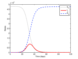
(a) Human population.

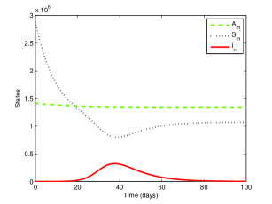
(b) Mosquito population.

Figure 1: State variables of the ODE system (1)–(2) with initial conditions (5) and parameters as in Table 1.

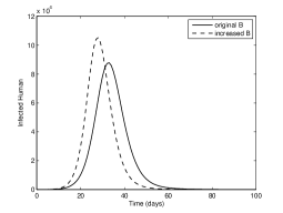
(a) Effect on $I_{h}$ of the variation of $B$.

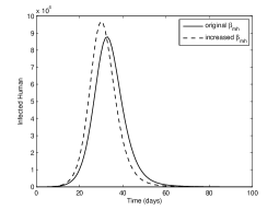
(b) Effect on $I_{h}$ of the variation of $\beta_{mh}$.

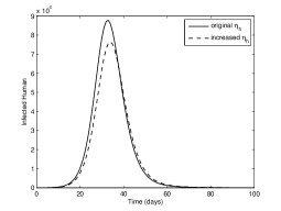
(c) Effect on $I_{h}$ of the variation of $\eta_{h}$.

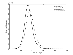
(d) Effect on $I_{h}$ of the variation of $\mu_{m}$.

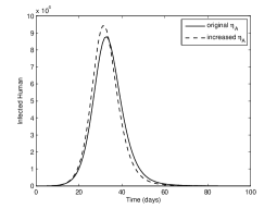
(e) Effect on $I_{h}$ of the variation of $\eta_{A}$.

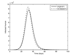
(f) Effect on $I_{h}$ of the variation of $k$.

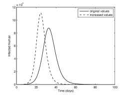
(g) Effect on $I_{h}$ when all parameters increase 10%.

Figure 2: Infected individuals with initial parameter values as given in Table 1 (solid line) and with an increase of 10% of a specific (or all, in g) parameter (dashed line).

6 Conclusions

A dengue model was studied by evaluating the sensitivity indices of the basic reproduction number, $\mathcal{R}_{0}$, in order to determine the relative importance of the model parameters in the disease transmission. Such information allow us to identify the robustness of the model predictions with respect to parameter values, the influence of each parameter in the basic reproduction number, and consequently in the disease evolution. Such analysis can provide critical information for decision makers and public health officials, who may have to deal with the reality of an infectious disease.

We trust that the research direction here initiated can be of great benefit to citizens affected by dengue, with an impact on both the prevention and control of an epidemic. Such contribution is especially interesting regarding a disease like dengue, which causes a large disruption in the lives of sufferers and has enormous social and economic costs, as was well illustrated by the outbreak of dengue that occurred in Cape Verde in 2009.

References

- [1] WHO. Dengue: guidelines for diagnosis, treatment, prevention and control. World Health Organization, 2nd edition, 2009.
- [2] S. C. Chen, and M. H. Hsieh. Modeling the transmission dynamics of dengue fever: implications of temperature effects. Sci. Total Environ., 431:385–391, 2012.
- [3] P. M. Luz, C. T. Codeço, E. Massad, and C. J. Struchiner. Uncertainties regarding dengue modeling in Rio de Janeiro, Brazil. Mem. Inst. Oswaldo Cruz, 98(7):871–878, 2003.
-
[4]
C. J. Silva, and D. F. M. Torres.
Optimal control for a tuberculosis model
with reinfection and post-exposure interventions.
Math. Biosci., 2013. arXiv:1305.2145
http://dx.doi.org/10.1016/j.mbs.2013.05.005 - [5] Y. Dumont, and F. Chiroleu. Vector control for the chikungunya disease. Math. Biosci. Eng., 7(2):313–345, 2010.
- [6] Y. Dumont, F. Chiroleu, and C. Domerg. On a temporal model for the chikungunya disease: modeling, theory and numerics. Math. Biosci., 213(1):80–91, 2008.
- [7] H. S. Rodrigues, M. T. T. Monteiro, and D. F. M. Torres. Optimization of dengue epidemics: a test case with different discretization schemes. AIP Conf. Proc., 1168(1):1385–1388, 2009. arXiv:1001.3303
- [8] H. S. Rodrigues, M. T. T. Monteiro, and D. F. M. Torres. Insecticide control in a dengue epidemics model. AIP Conf. Proc. 1281(1):979–982, 2010. arXiv:1007.5159
- [9] H. S. Rodrigues, M. T. T. Monteiro, D. F. M. Torres, and A. Zinober. Dengue disease, basic reproduction number and control. Int. J. Comput. Math., 89(3):334–346, 2012. arXiv:1103.1923
- [10] J. R. Heffernan, R. J. Smith, and L. M. Wahl. Perspective on the basic reproductive ratio. J. R. Soc. Interface, 2:281–293, 2005.
- [11] P. van den Driessche, and J. Watmough. Reproduction numbers and sub-threshold endemic equilibria for compartmental models of disease transmission. Math. Biosci., 180:29–48, 2002.
-
[12]
H. S. Rodrigues, M. T. T. Monteiro, and D. F. M. Torres.
Bioeconomic perspectives to an optimal control dengue model.
Int. J. Comput. Math., 2013. arXiv:1303.6904
http://dx.doi.org/10.1080/00207160.2013.790536 - [13] D. R. Powell, J. Fair, R. J. LeClaire, L. M. Moore, and D. Thompson. Sensitivity analysis of an infectious disease model. International System Dynamics Conference, Boston, MA, 2005.
- [14] N. Chitnis, J.M . Hyman, and J. M. Cusching. Determining important parameters in the spread of malaria through the sensitivity analysis of a mathematical model. Bull. Math. Biol., 70(5):1272–1296, 2008.
- [15] M. A Mikucki. Sensitivity analysis of the basic reproduction number and other quantities for infectious disease models. M.Sc. thesis, Colorado State University, 2012.