Optimal and sub-optimal quadratic forms for non-centered Gaussian processes

Abstract

Individual random trajectories of stochastic processes are often analyzed by using quadratic forms such as time averaged (TA) mean square displacement (MSD) or velocity auto-correlation function (VACF). The appropriate quadratic form is expected to have a narrow probability distribution in order to reduce statistical uncertainty of a single measurement. We consider the problem of finding the optimal quadratic form that minimizes a chosen cumulant moment (e.g., the variance) of the probability distribution, under the constraint of fixed mean value. For discrete non-centered Gaussian processes, we construct the optimal quadratic form by using the spectral representation of the cumulant moments. Moreover, we obtain a simple explicit formula for the smallest achievable cumulant moment that may serve as a quality benchmark for other quadratic forms. We illustrate the optimality issues by comparing the optimal variance with the variances of the TA MSD and TA VACF of fractional Brownian motion superimposed with a constant drift and independent Gaussian noise.

I Introduction

The statistical analysis and reliable interpretation of stochastic processes have become indispensable tools in fields as different as non-equilibrium statistical physics, biophysics, geophysics, ecology and finances. Examples range from random trajectories of individual tracers in living cells Saxton97b ; Tolic04 ; Golding06 ; Arcizet08 ; Wirtz09 ; Metzler09 ; Jeon11 ; Bertseva12 to market stock prices Bouchaud . The acquired trajectories are often unique, either due to the challenges in reconducting an experiment or reproducing the identical experimental conditions (e.g., in living cells), or due to the intrinsic uniqueness of the phenomenon (e.g., stock prices). In both cases, a single realization of the stochastic process has to be analyzed. Although the problem of optimal inferences has been thoroughly studied in statistics for a long time, none of various statistical tools is known to be universally the “best”. For instance, the maximum likelihood estimators are known to be (nearly) optimal but their implementation may be too time-consuming or impractical under certain circumstances. In turn, a much simpler tool of the time averaged (TA) mean square displacement (MSD) which is broadly used by experimentalists, may be biased or strongly non-optimal. The presence of localization errors, blurring, electronic noises and other acquisition artifacts may strongly alter the inferred parameters Berglund10 ; Michalet10 ; Michalet12 . As a consequence, the search for optimal inferences is still active, even for simple and well studied processes such as, e.g., Brownian motion Voisinne10 ; Grebenkov11b ; Boyer12a ; Boyer12b .

In this paper, we consider a discrete Gaussian process of $N$ steps, i.e., a Gaussian vector ${\bf x}=(x_{1},...,x_{N})^{\dagger}\in{\mathbb{R}}^{N}$, which is determined by given mean vector ${\bf x}^{0}$ and covariance matrix ${\bf C}$. In general, the mean vector and the covariance matrix are not known and have to be inferred from random realizations of the process. Such an inference of $N+N(N-1)/2$ unknowns is obviously impossible from a single realization of $N$ random points $x_{j}$. In many cases, however, the structure of the mean vector and/or the covariance matrix is expected. For instance, one-dimensional discrete Brownian motion (or off-lattice random walk) with a constant drift is defined by setting ${\bf x}^{0}=(a+\mu,a+2\mu,...,a+N\mu)$ and ${\bf C}_{j,k}=\sigma^{2}\min\{j,k\}$, where $a$ is the starting point, $\mu$ is the drift over one step (i.e., $\mu=v\delta$ where $\delta$ is the step duration and $v$ the velocity), and $\sigma^{2}$ is the one step variance (which is related to the diffusion coefficient $D$ as $\sigma^{2}=2D\delta$). Choosing a particular class of processes (i.e., choosing the structure for ${\bf x}^{0}$ and ${\bf C}$), one significantly reduces the number of unknowns, making the inference from a single realization tractable. For instance, only three parameters $a$, $\mu$ and $\sigma$ have to be inferred in the above example.

Many standard estimators employed for the analysis of single-particle trajectories operate with quadratic forms, $\chi=\frac{1}{2}({\bf x}^{\dagger}{\bf M}{\bf x})$, defined by a convenient symmetric matrix ${\bf M}$. Examples are TA MSD, TA VACF, power spectral density, squared root mean square displacements, etc. Grebenkov11a ; Grebenkov11b . Why different quadratic forms have been employed? How can one choose between them? What is the “best” quadratic form to infer the parameters of a known stochastic process? The answers to these questions strongly depend on the studied process and on the chosen optimality criterion.

Inspired by these questions, we consider here a more specific problem of finding the “optimal” symmetric matrix ${\bf M}_{\rm opt}$ that would minimize the variance $\kappa_{2}$ (or another cumulant moment $\kappa_{m}$) of the quadratic form $\chi$, under the constraint for the mean value $\kappa_{1}$ of $\chi$ to be fixed. In Grebenkov11b , we briefly mentioned this problem and showed that the optimal matrix ${\bf M}_{\rm opt}$ for discrete centered Gaussian processes (i.e., for ${\bf x}^{0}=0$) is proportional to the inverse of the covariance matrix ${\bf C}$: ${\bf M}_{\rm opt}=\lambda{\bf C}^{-1}$, with $\lambda=2\kappa_{1}/N$. In this case, the quadratic form $\chi$ has a Gamma distribution:

$$p(z)=\frac{z^{N/2-1}~{}e^{-z/\lambda}}{\Gamma(N/2)\lambda^{N/2}}.$$ (1)

For instance, the optimal quadratic form for discrete Brownian motion corresponds to the TA MSD with the unit time lag:

$$\frac{1}{2}({\bf x}^{\dagger}{\bf M}_{\rm opt}{\bf x})=\frac{\sigma^{2}}{N}({\bf x}^{\dagger}{\bf C}^{-1}{\bf x})=\frac{1}{N}\sum_{k=1}^{N}(x_{k}-x_{k-1})^{2}$$ (2)

(with $x_{0}=0$). This results agrees with the general Cramér-Rao lower bound which is achieved by the TA MSD with the unit lag time Cramer ; Voisinne10 . Moreover, this optimal choice minimizes simultaneously all cumulant moments $\kappa_{m}$ with $m\geq 2$.

In this paper, we extend this analysis to discrete non-centered Gaussian processes, for instance, in the presence of drift. We construct the optimal symmetric matrix ${\bf M}_{\rm opt}$ for given mean vector ${\bf x}^{0}$ and covariance matrix ${\bf C}$. We also derive a simple explicit formula for the smallest achievable cumulant moment that may serve as a quality benchmark for other quadratic forms. In particular, we compare the optimal matrix ${\bf M}_{\rm opt}$ (which depends on both ${\bf C}$ and ${\bf x}^{0}$), to a sub-optimal matrix $\propto{\bf C}^{-1}$ which is independent of ${\bf x}^{0}$ and thus more robust against uncertainties in ${\bf x}^{0}$ (which is often unknown or difficult to estimate accurately). We show that the variance (or higher cumulant moments) increases by a small amount when the sub-optimal matrix is used. Finally, we compare the optimal matrix to the standard quadratic estimators: TA MSD and TA VACF. For this purpose, we consider a discrete fractional Brownian motion (fBm) superimposed with a constant drift and independent Gaussian noise, as an archetypical model of anomalous transport affected by measurement artifacts such as drift and noise. For this Gaussian process, we compute analytically the mean and variance of the TA MSD and TA VACF, and compare them to the optimal matrix.

II Distribution of quadratic forms

In this section, we summarize the basic steps for computing the distribution of the quadratic form

$$\chi=\frac{1}{2}({\bf x}^{\dagger}{\bf M}{\bf x}),$$

which is defined by a given symmetric matrix ${\bf M}\in{\mathbb{R}}^{N}\times{\mathbb{R}}^{N}$. A discrete Gaussian process ${\bf x}=\{x_{1},...,x_{N}\}\in{\mathbb{R}}^{N}$ is characterized by its mean vector ${\bf x}^{0}=\{x_{1}^{0},...,x_{N}^{0}\}\in{\mathbb{R}}^{N}$ and the covariance matrix ${\bf C}$:

$$x^{0}_{n}=\langle x_{n}\rangle,\qquad{\bf C}_{n_{1}n_{2}}=\langle x_{n_{1}}x_{n_{2}}\rangle-\langle x_{n_{1}}\rangle\langle x_{n_{2}}\rangle,$$

where $\langle\cdots\rangle$ denotes the expectation with respect to the Gaussian probability density of ${\bf x}$:

$$P_{N}({\bf x})=\frac{1}{(2\pi)^{N/2}\sqrt{\det{\bf C}}}\exp\biggl{[}-\frac{1}{2}({\bf x}-{\bf x}^{0})^{\dagger}{\bf C}^{-1}({\bf x}-{\bf x}^{0})\biggr{]}.$$ (3)

The characteristic function of the quadratic form $\chi$ is easily found by regrouping two quadratic forms and computing Gaussian integrals:

$$\begin{split}&\phi(k)\equiv\langle e^{ik\chi}\rangle=\frac{1}{\sqrt{\det({\bf I}-ik{\bf M}_{\bf C})}}\times\\ &\exp\biggl{[}-\frac{1}{2}{\bf x}^{0,{\dagger}}{\bf C}^{-1/2}\bigl{[}{\bf I}-({\bf I}-ik{\bf M}_{\bf C})^{-1}\bigr{]}{\bf C}^{-1/2}{\bf x}^{0}\biggr{]},\\ \end{split}$$ (4)

where ${\bf M}_{\bf C}\equiv{\bf C}^{1/2}{\bf M}{\bf C}^{1/2}$, and the inverse and square root matrices of ${\bf C}$ are well defined as the covariance matrix ${\bf C}$ is symmetric and positive definite . The probability density $p(z)$ of the random variable $\chi$ can be retrieved through the inverse Fourier transform of $\phi(k)$:

$$p(z)=\int\limits_{-\infty}^{\infty}\frac{dk}{2\pi}e^{-ikz}\phi(k).$$ (5)

In practice, this computation can be rapidly performed by a fast Fourier transform. These basic formulas allow one to study various quadratic forms of discrete Gaussian processes. Note that the probability distribution of quadratic forms of Gaussian processes has been thoroughly studied in mathematical and physical literature (see a short overview in Grebenkov11b ).

The characteristic function $\phi(k)$ can be expressed through the spectral properties of the matrix ${\bf M}_{\bf C}$. Since the square root matrix ${\bf C}^{1/2}$ can be chosen to be symmetric, the matrix ${\bf M}_{\bf C}$ is symmetric and thus diagonalizable by an orthogonal matrix ${\bf U}$: ${\bf M}_{\bf C}={\bf U\Lambda U}^{\dagger}$, where ${\bf\Lambda}$ is a diagonal matrix. One gets therefore

$$\ln\phi(k)=-\frac{1}{2}\sum\limits_{q=1}^{N}\biggl{[}\ln(1-ik\lambda_{q})+c_{q}^{2}\bigl{(}1-(1-ik\lambda_{q})^{-1}\bigr{)}\biggr{]},$$ (6)

where $c_{q}\equiv({\bf x}^{0,{\dagger}}{\bf C}^{-1/2}{\bf U})_{q}$, and $\lambda_{q}$ are the eigenvalues of ${\bf M}_{\bf C}$. The logarithm of $\phi(k)$ is the generating function for the cumulant moments $\kappa_{m}\equiv\langle\chi^{m}\rangle_{c}$:

$$\ln\phi(k)=\sum\limits_{m=1}^{\infty}\frac{(ik)^{m}}{m!}\kappa_{m}.$$

Developing the logarithm in Eq. (6) into a Taylor series and identifying the coefficients, one finds

$$\kappa_{m} = \frac{m!}{2}\sum\limits_{q=1}^{N}\lambda_{q}^{m}\biggl{(}\frac{1}{m}+c_{q}^{2}\biggr{)}$$ (7)

$$= \frac{m!}{2}\biggl{[}\frac{{\rm tr}(({\bf M}{\bf C})^{m})}{m}+\bigl{(}{\bf x}^{0,{\dagger}}({\bf M}{\bf C})^{m-1}{\bf M}{\bf x}^{0})\biggr{]}.$$ (8)

For instance, $\kappa_{1}=\frac{1}{2}{\rm tr}({\bf M}{\bf C})+\frac{1}{2}({\bf x}^{0,{\dagger}}{\bf M}{\bf x}^{0})$ and $\kappa_{2}=\frac{1}{2}{\rm tr}(({\bf M}{\bf C})^{2})+({\bf x}^{0,{\dagger}}{\bf M}{\bf C}{\bf M}{\bf x}^{0})$ are the mean and the variance of $\chi$, respectively. The skewness and kurtosis are also expressed in terms of the cumulant moments as $\kappa_{3}/\kappa_{2}^{3/2}$ and $\kappa_{4}/\kappa_{2}^{2}$, respectively. Note that the moments $\langle\chi^{m}\rangle$ can be easily expressed through the cumulant moments, while the negative-order moments $\langle\chi^{-\alpha}\rangle$ can be obtained as the Mellin transform of the characteristic function (see Grebenkov11b for details). The spectral representations (6, 7) extend the analysis of Ref. Grebenkov11b to non-centered Gaussian processes with nonzero mean ${\bf x}_{0}$ which enters through the coefficients $c_{q}$.

III Optimal quadratic form

The representation (7) allows us to tackle the problem of finding the symmetric matrix ${\bf M}_{\rm opt}$ (to be called “optimal”) that minimizes a chosen cumulant moment $\kappa_{m}$ of the random variable $\chi$, under constraint of the mean value $\kappa_{1}$ to be fixed. For centered Gaussian processes (${\bf x}^{0}=0$), we showed that the optimal choice is achieved when all eigenvalues $\lambda_{q}$ of the matrix ${\bf M}_{\bf C}$ are identical (and equal to $\lambda=2\kappa_{1}/N$), from which ${\bf M}_{\rm opt}=\lambda{\bf C}^{-1}$ Grebenkov11b . In this paper, we extend this result to non-centered Gaussian processes.

A formal solution of the minimization problem for a given cumulant moment $\kappa_{m}$ leads to a system of $N\times N$ equations on the elements of the matrix ${\bf M}$:

$$\frac{\partial}{\partial{\bf M}_{jk}}\biggl{[}\kappa_{m}+\alpha\biggl{(}2\kappa_{1}-\bigl{[}{\rm tr}({\bf M}{\bf C})+({\bf x}^{0,{\dagger}}{\bf M}{\bf x}^{0})\bigr{]}\biggr{)}\biggr{]}=0,$$

where the second term incorporates the constraint (with the Lagrange multiplier $\alpha$), and $\kappa_{m}$ is expressed in terms of ${\bf M}$ according to Eq. (8). This system is linear only for $m=2$. Although a numerical solution of the system is possible for small $N$, it does not help to understand the properties of the optimal solution in general.

The key point of the following analysis is the spectral representation (7) of the cumulant moment $\kappa_{m}$ in terms of $\lambda_{q}$ and $c_{q}$. The eigenvalues $\lambda_{q}$ determine the diagonal matrix ${\bf\Lambda}$, while $c_{q}$ are the projections of a given vector ${\bf C}^{-1/2}{\bf x}^{0}$ onto the columns of the orthogonal matrix ${\bf U}$. The constrained minimization of $\kappa_{m}$ is equivalent to unconstrained minimization of the function

$$\begin{split}f&=\sum\limits_{q}\lambda_{q}^{m}(1+mc_{q}^{2})\\ &+\alpha\biggl{(}2\kappa_{1}-\sum\limits_{q}\lambda_{q}(1+c_{q}^{2})\biggr{)}+\beta\biggl{(}\sum\limits_{q}c_{q}^{2}-\gamma\biggr{)}.\\ \end{split}$$ (9)

with respect to $\lambda_{q}$ and $c_{q}$. Here $\alpha$ and $\beta$ are two Lagrange multipliers that implement two constraints:

$$\sum\limits_{q}\lambda_{q}(1+c_{q}^{2}) = 2\kappa_{1},$$ (10)

$$\sum\limits_{q}c_{q}^{2} = ({\bf x}^{0,{\dagger}}{\bf C}^{-1}{\bf x}^{0})\equiv\gamma.$$ (11)

The first constraint eliminates a trivial solution ${\bf M}=0$ that would minimize all the cumulant moments. The second relation accounts for the orthogonality of the matrix ${\bf U}$.

In what follows, we consider $m\geq 2$ to be even, in order to ensure that the function $f$ is bounded from below and thus admits a minimum. Setting the derivatives of $f$ with respect to $\lambda_{q}$ and $c_{q}$ to zero yields two sets of equations:

$$m\lambda_{q}^{m-1}(1+mc_{q}^{2})-\alpha(1+c_{q}^{2}) = 0,$$ (12)

$$(m\lambda_{q}^{m}-\alpha\lambda_{q}+\beta)c_{q} = 0,$$ (13)

which are completed by the constraints (10, 11). The first equation yields

$$\lambda_{q}=\lambda\left(\frac{1+c_{q}^{2}}{1+mc_{q}^{2}}\right)^{\frac{1}{m-1}},\qquad\lambda\equiv\left(\frac{\alpha}{m}\right)^{\frac{1}{m-1}}.$$ (14)

The second equation admits two options:

(i) $c_{q}^{2}=0$, for which $\lambda_{q}=\lambda$ according to Eq. (14);

(ii) $c_{q}^{2}>0$, in which case one has to solve the equation

$$m\lambda_{q}^{m}-\alpha\lambda_{q}+\beta=0.$$ (15)

Since $\alpha$ and $\beta$ are constants (to be determined), solutions of this equation have the same form for all $q$. In general, the $m$-th order polynomial in Eq. (15) has $m$ (complex-valued) roots. In Appendix A, we show that only one root of Eq. (15) is compatible with Eq. (14).

There is still a freedom to choose one of two above options for every $q$. Let $Q$ denote the number of nonzero coefficients $c_{q}^{2}$. The statement of Appendix A implies that $\lambda_{1}=...=\lambda_{Q}$ and thus $c_{1}^{2}=...=c_{Q}^{2}>0$. For the remaining indices $q=Q+1,...,N$, one has $c_{q}^{2}=0$ and $\lambda_{q}=\lambda$. Substituting these relations in Eqs. (10, 11) yields $c_{1}^{2}=\gamma/Q$ and

$$2\kappa_{1}=\sum\limits_{q}\lambda_{q}(1+c_{q}^{2})=Q\lambda_{1}(1+\gamma/Q)+(N-Q)\lambda,$$

from which

$$\lambda_{1}=\frac{2\kappa_{1}-(N-Q)\lambda}{Q+\gamma}.$$

Comparing this relation with Eq. (14) leads to

$$\lambda=\frac{2\kappa_{1}}{(Q+\gamma)\left(\frac{Q+\gamma}{Q+m\gamma}\right)^{\frac{1}{m-1}}+(N-Q)},$$ (16)

so that

$$\lambda_{q}=\lambda\times\begin{cases}\left(\frac{Q+\gamma}{Q+m\gamma}\right)^{\frac{1}{m-1}},\quad q=1,...,Q,\cr~{}\hskip 17.07164pt1,\hskip 42.67912ptq=Q+1,...,N.\end{cases}$$ (17)

In other words, the fact that only one solution of Eq. (15) is admissible allows us to omit resolution of this equation.

For centered processes (i.e., ${\bf x}^{0}=0$ and $\gamma=0$), one retrieves $\lambda_{q}=\lambda=2\kappa_{1}/N$ that minimized all the cumulant moments. In contrast, when $\gamma>0$, the optimal solution $\lambda_{q}$ depends on the order $m$ of the moment to be minimized.

The $n$-th cumulant moment for the optimal form reads according to Eq. (7) as

$$\kappa_{n}^{\rm opt}=\frac{(n-1)!}{2}\lambda^{n}\biggl{[}\left(\frac{Q+\gamma}{Q+m\gamma}\right)^{\frac{n}{m-1}}(Q+n\gamma)+(N-Q)\biggr{]},$$ (18)

where $n$ may be different from $m$. When $n=m$, one gets

$$\kappa_{m}^{\rm opt}=\frac{(m-1)!}{2}\lambda^{m-1}2\kappa_{1}.$$ (19)

In particular, one has for $m=n=2$

$$\kappa_{2}^{\rm opt}=\frac{2\kappa_{1}^{2}}{N}\biggl{(}1+\frac{\gamma^{2}}{N(Q+2\gamma)}\biggr{)}^{-1}.$$ (20)

The function $\kappa_{m}^{\rm opt}$ monotonously increases with $Q$ because

$$\frac{\partial\lambda}{\partial Q}=\frac{\lambda^{2}}{2\kappa_{1}}\biggl{[}1-\left(\frac{Q+\gamma}{Q+m\gamma}\right)^{\frac{1}{m-1}}\frac{Q+\gamma(m+1)}{Q+m\gamma}\biggr{]}\geq 0,$$

that follows from the inequality

$$(1+z(m+1))^{m-1}(1+z)\leq(1+mz)^{m},$$

where $z=\gamma/(Q+\gamma)$ lies between $0$ and $1$. As a consequence, the minimum of the $m$-th cumulant moment is reached for $Q=1$. In particular, Eqs. (16, 19) with $Q=1$ give a simple explicit formula for the smallest achievable cumulant moment.

Note also that nonzero mean vector (e.g., a drift) always diminishes the optimal cumulant moment $\kappa_{m}^{\rm opt}$ because

$$\frac{\partial\lambda}{\partial\gamma}=-\frac{m\gamma\lambda^{2}}{2\kappa_{1}}~{}\frac{(Q+\gamma)^{\frac{1}{m-1}}}{(Q+m\gamma)^{\frac{m}{m-1}}}<0.$$

In addition, the parameter $\lambda$ and thus the optimal moment $\kappa_{m}^{\rm opt}$ go to $0$ as $\gamma\to\infty$ according to Eqs. (16, 19). In fact, the contribution of the mean vector ${\bf x}^{0}$ strongly dominates over random fluctuations in this limit. We emphasize again that this statement remains correct only under the constraint of fixed mean value.

When the mean vector ${\bf x}^{0}$ and covariance matrix ${\bf C}$ are known, the optimal matrix ${\bf M}_{\rm opt}$ can be constructed as follows. First, one sets the vector ${\bf u}_{1}={\bf C}^{-1/2}{\bf x}^{0}/\sqrt{\gamma}$ and then chooses $N-1$ orthonormal vectors ${\bf u}_{q}$ ($q=2,...,N$) that are all orthogonal to ${\bf u}_{1}$ so that $c_{q}=({\bf u}_{q}\cdot{\bf C}^{-1/2}{\bf x}^{0})=({\bf u}_{q}\cdot\sqrt{\gamma}{\bf u}_{1})=0$. By construction, $c_{1}=({\bf u}_{1}\cdot{\bf C}^{-1/2}{\bf x}^{0})=({\bf x}^{0,{\dagger}}{\bf C}^{-1}{\bf x}^{0})/\sqrt{\gamma}=\sqrt{\gamma}$. The vectors ${\bf u}_{q}$ form the orthogonal matrix ${\bf U}$. After that, one constructs a diagonal matrix ${\bf\Lambda}$ which has the first element $\lambda_{1}=\lambda\bigl{(}\frac{1+\gamma}{1+m\gamma}\bigr{)}^{\frac{1}{m-1}}$ and the other diagonal elements $\lambda_{q}=\lambda$, with $\lambda$ from Eq. (16) with $Q=1$. One gets therefore

$$[{\bf U}{\bf\Lambda}{\bf U}^{+}]_{j,k}=\lambda\delta_{j,k}+\frac{\lambda_{1}-\lambda}{\gamma}({\bf C}^{-1/2}{\bf x}^{0})_{j}({\bf C}^{-1/2}{\bf x}^{0})_{k},$$

from which the identity ${\bf M}={\bf C}^{-1/2}{\bf U}{\bf\Lambda}{\bf U}^{\dagger}{\bf C}^{-1/2}$ yields the optimal matrix ${\bf M}_{\rm opt}$ as

$$[{\bf M}_{\rm opt}]_{j,k}=\lambda[{\bf C}^{-1}]_{j,k}-\frac{\eta}{\gamma}({\bf C}^{-1}{\bf x}^{0})_{j}({\bf C}^{-1}{\bf x}^{0})_{k},$$ (21)

with

$$\eta\equiv\lambda-\lambda_{1}=\lambda\biggl{(}1-\biggl{(}\frac{1+\gamma}{1+m\gamma}\biggr{)}^{\frac{1}{m-1}}\biggr{)}.$$ (22)

One can see how the mean vector ${\bf x}^{0}$ modifies the optimal matrix through the prefactor $\lambda$ [given by Eq. (16)] and the second term in Eq. (21).

Sub-optimal matrix

A limitation of the above approach is the need for knowing the covariance matrix ${\bf C}$ and the mean vector ${\bf x}^{0}$. In particular, the resulting optimal matrix ${\bf M}_{\rm opt}$ depends not only on the structure of ${\bf C}$ and ${\bf x}^{0}$, but also on the parameters (e.g., the drift coefficient) which are often unknown and have to be inferred. For inference purposes, one needs to find such a matrix ${\bf M}_{\rm sub}$ which may be sub-optimal but more robust against changes of the parameters. Quite remarkably, one can check that the optimal moment $\kappa_{m}^{\rm opt}$ from Eq. (19) weakly depends on $Q$. In the “worst” case $Q=N$, the diagonal matrix ${\bf\Lambda}$ is simply proportional to the identity matrix, ${\bf\Lambda}=\frac{2\kappa_{1}}{N+\gamma}{\bf I}$, so that the related sub-optimal matrix becomes

$${\bf M}_{\rm sub}=\frac{2\kappa_{1}}{N+\gamma}{\bf C}^{-1}.$$ (23)

The crucial simplification here is that the mean vector ${\bf x}^{0}$ enters only through the prefactor $1/(N+\gamma)$ in front of ${\bf C}^{-1}$. In other words, the structure of the matrix ${\bf M}_{\rm sub}$ does not depend on the particular structure of the mean vector. Although the matrix ${\bf M}_{\rm sub}$ is less optimal than ${\bf M}_{\rm opt}$, the difference between the $m$-th cumulant moments for both matrices is small. For instance, when $m=2$, the difference between the variances of the optimal and sub-optimal quadratic forms can be found from Eq. (20) as

$$\kappa_{2}^{\rm sub}-\kappa_{2}^{\rm opt}=\frac{2\kappa_{1}^{2}(N-1)\gamma^{2}}{(N^{2}+2\gamma N+\gamma^{2})(N+2\gamma N+\gamma^{2})}.$$

This difference vanishes at $\gamma=0$ and $\gamma\to\infty$, attending the maximum value $\approx 0.09(2\kappa_{1}^{2}/N)$ at $\gamma\approx\frac{\sqrt{5}-1}{2}~{}N$ (for large $N$). One concludes that the use of the sub-optimal matrix ${\bf M}_{\rm sub}$ instead of ${\bf M}_{\rm opt}$ may increase the variance by at most $\approx 10\%$.

IV Fractional Brownian motion

As we discussed earlier, the TA MSD with the lag time $n=1$ is the optimal quadratic functional for Brownian motion. The simplicity of the TA MSD made this quadratic functional broadly employed for the analysis of more sophisticated processes such as anomalous diffusions. Various types of motion in living cells, biological tissues and mineral samples were observed and analyzed: restricted, obstructed and hindered diffusion, directed motion, anomalous diffusion, diffusion through traps, etc. Saxton97b ; Saxton93 ; Metzler09 ; Bouchaud90 ; Metzler00 ; Grebenkov07 . One may wonder how strongly the efficiency of the TA MSD for other Gaussian processes is reduced as compared to the optimal quadratic form. In other words, it is instructive to compare the variance of the TA MSD for anomalous diffusion to the optimal variance $\kappa_{2}^{\rm opt}$ from Eq. (20). Given that the optimal variance was obtained under the constraint of fixed mean $\kappa_{1}$, it is convenient to consider the ratio $\kappa_{2}/\kappa_{1}^{2}$. Note that this ratio for TA MSD was also called “ergodicity breaking parameter” and thoroughly studied for anomalous diffusions Deng09 ; Jeon10 ; Jeon11 ; Burov11 . In particular, the behavior of this ratio in the limit $N\to\infty$ would tell about ergodic properties of the system: if this ratio vanishes as $N\to\infty$, the time average over infinitely long trajectory is equivalent to the ensemble average (the ergodic property); in turn, the nonzero limit indicates weak ergodicity breaking which was observed and investigated for different kinds of continuous-time random walks (see Burov11 and references therein).

As an archetypical model of anomalous diffusion, we consider a (discrete) fractional Brownian motion with the Hurst exponent $0<H<1$ (its continuous version was introduced by Kolmogorov Kolmogorov40 and later by Mandelbrot and van Ness Mandelbrot68 ). We also add a constant drift $\mu$ and an independent Gaussian noise with mean zero and variance $\varepsilon^{2}$ that may account for some measurement artifacts Berglund10 ; Michalet10 ; Michalet12 . The resulting process (starting from $0$) is still Gaussian and thus fully characterized by the mean vector ${\bf x}^{0}=\mu(1,2,...,N)^{\dagger}$ and the covariance matrix

$${\bf C}_{n_{1},n_{2}}=\frac{\sigma^{2}}{2}\bigl{(}n_{1}^{2H}+n_{2}^{2H}-|n_{1}-n_{2}|^{2H}\bigr{)}+\varepsilon^{2}\delta_{n_{1},n_{2}}.$$ (24)

The fBm is persistent (with positive correlations between steps) or anti-persistent (with negative correlations between steps) for $H>1/2$ and $H<1/2$, respectively. Finally, one retrieves Brownian motion at $H=1/2$.

IV.1 Optimal variance

In contrast to Brownian motion, the inverse matrix ${\bf C}^{-1}$ is not known explicitly for fBm. Setting $\varepsilon=0$ for simplicity, we check numerically that the coefficient $\gamma$ defined by Eq. (11) behaves as $\gamma\approx\frac{\mu^{2}}{\sigma^{2}}N^{2(1-H)}(c_{H}+O(1/N))$, where the constant $c_{H}$ is close to $1$ and weakly dependent on $H$ when $H$ is not too small. According to Eq. (20), we get the optimal ratio

$$\frac{\kappa_{2}^{\rm opt}}{2\kappa_{1}^{2}}\simeq\frac{1}{N}\left(1+\frac{\mu^{4}c_{H}^{2}}{\sigma^{4}}\frac{N^{3-4H}}{1+2\frac{\mu^{2}}{\sigma^{2}}N^{2(1-H)}}\right)^{-1}.$$ (25)

Two limiting cases of small and large drift $\mu$, as compared to $\sigma N^{H-1}$, yield

$$\frac{\kappa_{2}^{\rm opt}}{2\kappa_{1}^{2}}\simeq\begin{cases}\frac{1}{N}\bigl{(}1+\frac{\mu^{4}c_{H}^{2}}{\sigma^{4}}N^{3-4H}\bigr{)}^{-1}\quad(\mu\ll\sigma N^{H-1}),\cr\frac{1}{N}\bigl{(}1+\frac{\mu^{2}c_{H}^{2}}{2\sigma^{2}}N^{1-2H}\bigr{)}^{-1}\quad(\mu\gg\sigma N^{H-1}).\end{cases}$$ (26)

Since $H<1$, the “border” $\sigma N^{H-1}$ between two asymptotic limits decreases with $N$. In addition, the drift “correction” may be either enhanced, or damped with $N$ for different values of $H$. For instance, when $H>1/2$, the second term in the second relation decreases, i.e., the role of the drift progressively diminishes. In turn, when $H<1/2$, the drift changes significantly the properties of the optimal quadratic form.

IV.2 Comparison with TA MSD

The TA MSD with the lag time $n$ over a sample of length $N$ is defined as a moving average

$$\chi=\frac{1}{N-n}\sum\limits_{k=1}^{N-n}(x_{k+n}-x_{k})^{2}$$ (27)

(note that this analysis is also applicable to multi-dimensional processes for which the TA MSD is simply the sum of TA MSDs for each component). One can notice that Eq. (27) with the lag time $n=1$ is slightly different from the optimal one defined by Eq. (2). In fact, the latter contains an additional term $(x_{1}-x_{0})^{2}=x_{1}^{2}$ and the prefactor $1/N$ instead of $1/(N-1)$. Nevertheless, we keep the definition (27) which is commonly used. All the presented results can be recomputed for Eq. (2) as well.

After lengthy computation, we obtain the mean and variance of the TA MSD for the discrete fBm with a constant drift and independent Gaussian noise:

$$\kappa_{1}=\sigma^{2}n^{2H}+\mu^{2}n^{2}+2\varepsilon^{2},$$ (28)

and

$$\begin{split}\kappa_{2}&=\frac{2}{N-n}\biggl{[}\sigma^{4}c_{\sigma,\sigma}n^{4H}+2\mu^{2}\sigma^{2}c_{\sigma,\mu}n^{2+2H}\\ &+4\mu^{2}\varepsilon^{2}c_{\mu,\varepsilon}n^{2}+4\varepsilon^{2}\sigma^{2}c_{\sigma,\varepsilon}n^{2H}+4\varepsilon^{4}c_{\varepsilon,\varepsilon}\biggr{]},\\ \end{split}$$ (29)

where

$$\begin{split}c_{\sigma,\sigma}(n,N)&=1+S_{H}^{(2)}(n,N),\\ c_{\sigma,\mu}(n,N)&=1+S_{H}^{(1)}(n,N),\\ c_{\mu,\varepsilon}(n,N)&=\begin{cases}\frac{n}{N-n}\quad(n<N/2),\cr 1\hskip 25.60747pt(n\geq N/2),\end{cases}\\ c_{\varepsilon,\varepsilon}(n,N)&=\begin{cases}\frac{3}{2}-\frac{n}{2(N-n)}\quad(n<N/2),\cr 1\hskip 54.06023pt(n\geq N/2),\end{cases}\\ c_{\sigma,\varepsilon}(n,N)&=\begin{cases}1-(2^{2H-1}-1)\frac{N-2n}{N-n}\quad(n<N/2),\cr 1\hskip 99.58464pt(n\geq N/2),\end{cases}\\ \end{split}$$

and

$$\begin{split}S_{H}^{(m)}(n,N)&\equiv\frac{1}{m~{}n^{2Hm}(N-n)}\sum\limits_{k=1}^{N-n-1}(N-n-k)\\ &\times\biggl{(}|k-n|^{2H}+|k+n|^{2H}-2k^{2H}\biggr{)}^{m}.\\ \end{split}$$ (30)

The general formulas (28, 29) allow one to study the dependence of the mean and variance of the TA MSD on different parameters of the studied process, namely, $H$, $\sigma$, $\mu$ and $\varepsilon$. In particular, we will investigate the behavior of the ratio $\kappa_{2}/(2\kappa_{1}^{2})$ for different situations.

Brownian motion

For $H=1/2$, the sum (30) can be computed explicitly, from which

$$c_{\sigma,\mu}(n,N)=\begin{cases}\frac{1+3Nn-4n^{2}}{3(N-n)}\hskip 48.36967pt(n<N/2),\cr\frac{1+3N(N-n)-4(N-n)^{2}}{3n}\quad(n\geq N/2),\end{cases}$$

and $c_{\sigma,\sigma}(n,N)=(N-n)F_{n,N}$, where the prefactor $F_{n,N}$ was first derived by Qian et al. Qian91 :

$$F_{n,N}=\begin{cases}\frac{4n^{2}N-5n^{3}+2N-n}{6n(N-n)^{2}}\hskip 82.51299pt(n\leq N/2),\cr\frac{(N-n)^{3}-4n(N-n)^{2}+6n^{2}(N-n)+5n-N}{6n^{2}(N-n)}\hskip 5.69054pt(n\geq N/2).\end{cases}$$

The prefactor $F_{n,N}$ is an increasing function of $n$ which ranges from $\frac{1}{N-1}$ at $n=1$ to $1$ at $n=N-1$.

When there is no drift ($\mu=0$), Eq. (29) is reduced to

$$\kappa_{2}=2n^{2}F_{n,N}+\frac{8n\varepsilon^{2}}{N-n}+\frac{8\varepsilon^{4}}{N-n}\times\begin{cases}\frac{3N-4n}{2(N-n)}~{}~{}(n\leq N/2),\cr 1\hskip 32.72066pt(n>N/2).\end{cases}$$

One can check that the ratio $\kappa_{2}/(2\kappa_{1}^{2})$ is an increasing function of $n$. As expected, the ratio is minimal for $n=1$, for which

$$\frac{\kappa_{2}}{2\kappa_{1}^{2}}=\frac{1}{N-1}\biggl{(}1+2\varepsilon^{4}\frac{1-\frac{3}{N-1}}{(1+2\varepsilon^{2})^{2}}\biggr{)}.$$

The noise monotonously increases the ratio, from the (almost) optimal value $\frac{1}{N-1}$ to approximately $\frac{3}{2}~{}\frac{1}{N-1}$ in the limit of very large noises. In turn, the optimal quadratic form obtained by inverting the matrix ${\bf C}$ from Eq. (24) would give the minimal ratio $1/N$.

As we mentioned earlier, the inverse of the covariance matrix ${\bf C}$ from Eq. (24) with $H=1/2$ and $\varepsilon=0$ (no noise) can be found explicitly, and ${\bf C}^{-1}$ determines the TA MSD with the unit lag time according to Eq. (2). As a consequence, one has $({\bf C}^{-1}{\bf x}_{0})_{j}=\mu\delta_{j,N}/\sigma^{2}$ so that $\gamma=\mu^{2}N/\sigma^{2}$, and the optimal matrix from Eq. (21) gets an explicit form

$$[{\bf M}_{\rm opt}]_{j,k}=\lambda[{\bf C}^{-1}]_{j,k}-\frac{\eta}{N\sigma^{2}}~{}\delta_{j,N}~{}\delta_{k,N}.$$ (31)

One can see that the drift term modifies the prefactor $\lambda$ in front of ${\bf C}^{-1}$ and also changes the last element of the matrix ${\bf M}_{\rm opt}$. We conclude

$$\frac{1}{2}({\bf x}^{\dagger}{\bf M}_{\rm opt}{\bf x})=\frac{\lambda}{2\sigma^{2}}\sum_{n=1}^{N}(x_{n}-x_{n-1})^{2}-\frac{\eta}{2N\sigma^{2}}x_{n}^{2}.$$

This explicit result is specific to discrete Brownian motion.

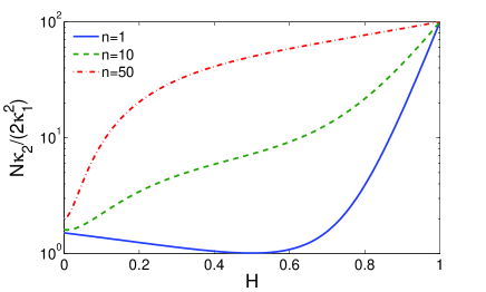
Figure 1: (Color online) The ratio $\kappa_{2}/(2\kappa_{1}^{2})$ for the TA MSD of the discrete fBm versus the Hurst exponent $H$ (with $N=100$, $\sigma=1$, $\mu=\varepsilon=0$), with different lag times: $n=1$ (blue solid line), $n=10$ (green dashed line) and $n=50$ (red dash-dotted line). This ratio is normalized by optimal value $1/N$.

Fractional Brownian motion

When $\mu=\varepsilon=0$, one gets

$$\frac{\kappa_{2}}{2\kappa_{1}^{2}}=\frac{c_{\sigma,\sigma}}{N-n}.$$ (32)

This ratio monotonously increases with $n$, i.e., for any $H$, the minimal ratio is achieved for $n=1$, as expected. Setting $n=1$, one checks that the positive sum $S_{H}^{(2)}(1,N)$ vanishes at $H=1/2$ that minimizes the ratio in Eq. (32). This is expected as the TA MSD with the unit lag time is optimal for Brownian motion. For $H<1/2$, the largest ratio corresponds to the limit $H=0$ and is equal to $\frac{1}{N-1}\bigl{(}\frac{3}{2}-\frac{1}{2(N-1)}\bigr{)}$ which is $50\%$ larger than the value $\frac{1}{N-1}$ at $H=1/2$. In contrast, this ratio rapidly increases for $H>1/2$, attending the value $1$ at $H=1$. The behavior of the ratio $\kappa_{2}/(2\kappa_{1}^{2})$ is illustrated on Fig. 1 for three lag times. We conclude that the TA MSD can still be applied to the analysis of subdiffusive fBm with $H<1/2$, while other quadratic functionals would significantly outperform the TA MSD for superdiffusive fBm with $H>1/2$.

It is also instructive to analyze the dependence of $\kappa_{2}/(2\kappa_{1}^{2})$ on the sample length $N$. For $n=1$, the sum $S_{H}^{(m)}(1,N)$ asymptotically behaves as $\propto N^{2m(H-1)+1}$ for large $N$. As a consequence, two different situations have to be distinguished: for $H<3/4$, the coefficient $c_{\sigma,\sigma}(1,N)$ converges to a constant as $N\to\infty$, while for $H>3/4$, it diverges as $\propto N^{4(H-3/4)}$ (for $H=3/4$, the divergence is logarithmic). In other words, for $H<3/4$, the statistical uncertainty remains of the order of $N^{-1}$ independently of $H$; in turn, for $H>3/4$, the decrease rate is dependent on $H$ and slower: $\propto N^{-4(1-H)}$. This behavior for continuous-time fBm was derived analytically by Deng and Barkai Deng09 (see also Jeon10 ).

The effect of drift and noise onto the variance $\kappa_{2}$ of the TA MSD may be quite sophisticated. First, the ratio $\kappa_{2}/\kappa_{1}^{2}$ is not necessarily minimal at the lag time $n=1$. For this reason, we consider the minimal value of the ratio $\kappa_{2}/(2\kappa_{1}^{2})$ over all lag times $n$ from $1$ to $N-1$. This ratio is then normalized by the optimal ratio $\kappa_{2}^{\rm opt}/(2\kappa_{1}^{2})$ that is equivalent to plotting $\kappa_{2}/\kappa_{2}^{\rm opt}$. By construction, the latter ratio is always greater than $1$. Small deviations from $1$ would mean nearly optimal inference power of the TA MSD. Figure 2 illustrates the optimality of the TA MSD for fBm altered by drift and noise. When drift coefficient $\mu$ or noise level $\varepsilon$ are large, the ratio $\kappa_{2}/\kappa_{2}^{\rm opt}$ is getting smaller and weakly dependent on $H$. This is not surprising as drift or noise dominates over fBm at large $\mu$ or $\varepsilon$. Interestingly, the drift shifts the minimum of the ratio towards $H<1/2$ (Fig. 2a), while the noise shifts the minimum towards $H>1/2$ (Fig. 2b).

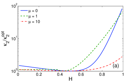
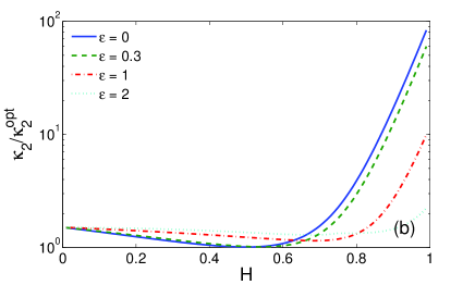
Figure 2: (Color online) The ratio $\kappa_{2}/\kappa_{2}^{\rm opt}$ for the TA MSD of the discrete fBm versus the Hurst exponent $H$ (with $N=100$, $\sigma=1$): (a) for three drifts $\mu$ (without noise, $\varepsilon=0$); (b) for four noise levels $\varepsilon$ (without drift, $\mu=0$). Here, one uses the minimal value of $\kappa_{2}$ over all lag times.

IV.3 Comparison with TA VACF

The velocity auto-correlation function, $\langle\dot{X}(t_{1})\dot{X}(t_{2})\rangle$, provides a direct measure of correlations between elementary displacements of the process. For the analysis of individual trajectories, the ensemble average has to be replaced by the time average of $\dot{X}(t_{0}+t)\dot{X}(t_{0})$ with a fixed lag time $t$ and $t_{0}$ sliding along the sample trajectory. In practice, the time derivative (denoted by dot) is approximated by a finite difference between the neighboring positions so that the discrete TA VACF is

$$\chi=\frac{1}{N-n-1}\sum\limits_{k=1}^{N-n-1}(x_{k+n+1}-x_{k+n})(x_{k+1}-x_{k})$$ (33)

(the factor $1/\delta^{2}$ is omitted for the sake of simplicity). Similarly to TA MSD, this expression defines a quadratic form $\frac{1}{2}({\bf x}^{{\dagger}}{\bf M}{\bf x})$ associated with a symmetric matrix ${\bf M}$ whose elements can be written explicitly.

We compute the mean and variance of the TA VACF for the discrete fractional Brownian motion with drift and noise:

$$\kappa_{1}=\frac{\sigma^{2}}{2}\biggl{[}(n+1)^{2H}+(n-1)^{2H}-2n^{2H}\biggr{]}+\mu^{2}-\varepsilon^{2}\delta_{n,1},$$ (34)

and

$$\kappa_{2}=\frac{\sigma^{4}\tilde{c}_{\sigma,\sigma}+\sigma^{2}\varepsilon^{2}\tilde{c}_{\sigma,\varepsilon}+\varepsilon^{4}\tilde{c}_{\varepsilon,\varepsilon}+\mu^{2}\sigma^{2}\tilde{c}_{\sigma,\mu}+\mu^{2}\varepsilon^{2}\tilde{c}_{\mu,\varepsilon}}{N-n-1},$$ (35)

with the explicit but lengthy formulas for the coefficients (dependent on $n$ and $N$) provided in Appendix B.

Brownian motion

For Brownian motion ($H=1/2$), the above expressions are simplified: $\tilde{c}_{\sigma,\sigma}=1$, $\tilde{c}_{\sigma,\varepsilon}=4$, and

$$\tilde{c}_{\sigma,\mu}=2+\begin{cases}2\frac{N-2n-1}{N-n-1}\quad(n<N/2),\cr 0,\hskip 39.83385pt(n\geq N/2).\end{cases}$$

When there is no drift and noise, the mean TA VACF is zero because all the displacements of Brownian motion are independent. Since the variance $\kappa_{2}=\frac{1}{N-n-1}$ is finite, the ratio $\kappa_{2}/(2\kappa_{1}^{2})$ is infinite. Clearly, the TA VACF (as well as any other quadratic form with zero mean) is far from being optimal because a measured empirical value does not allow one to infer any parameter of the process.

In the presence of drift, the mean value $\kappa_{1}=\mu^{2}$ (for $n>1$) allows one to estimate the drift coefficient. Neglecting noise, one gets

$$\frac{\kappa_{2}}{2\kappa_{1}^{2}}=\frac{\sigma^{2}}{N-n-1}\biggl{(}1+\frac{\sigma^{2}}{2\mu^{2}}+\max\biggl{\{}0,1-\frac{n}{N-n-1}\biggr{\}}\biggr{)},$$

which is minimal at $n=1$: $\frac{\kappa_{2}}{2\kappa_{1}^{2}}\approx\frac{\sigma^{2}}{N-2}\bigl{(}2+\frac{\sigma^{2}}{2\mu^{2}}\bigr{)}$.

Fractional Brownian motion

For fBm without noise and drift, the ratio $\kappa_{2}/(2\kappa_{1}^{2})$ is minimal for $n=1$ as expected. Figure 3 illustrates the behavior of this ratio as a function of $H$ (solid blue curve). One can observe the divergence at $H=1/2$ as mentioned earlier for Brownian motion.

In the presence of drift or noise, the ratio $\kappa_{2}/(2\kappa_{1}^{2})$ is not necessarily minimal for $n=1$. As for TA MSD, we first find the minimal value of $\kappa_{2}/(2\kappa_{1}^{2})$ over all lag times and then normalize it by the optimal ratio $\kappa_{2}^{\rm opt}/(2\kappa_{1}^{2})$. The behavior of the resulting ratio $\kappa_{2}/\kappa_{2}^{\rm opt}$ is shown on Fig. 3 for different drift coefficients $\mu$ and noise levels $\varepsilon$. As expected, there is no more divergence at $H=1/2$ because the mean TA VACF is not zero. Similarly to TA MSD, the ratio is getting smaller and weakly dependent on $H$ for large values of $\mu$ or $\varepsilon$. Moreover, the ratio becomes close to $1$ for large $\mu$. This behavior is expected from the very definition of the VACF as a measure of correlations between displacements; in particular, the VACF is constructed to access the drift.

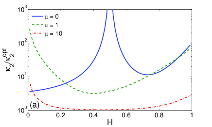
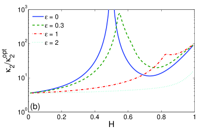
Figure 3: (Color online) The ratio $\kappa_{2}/\kappa_{2}^{\rm opt}$ for the TA VACF of the discrete fBm of the Hurst exponent $H$ (with $N=100$, $\sigma=1$). (a) For three drifts $\mu$ (without noise, $\varepsilon=0$); (b) for four noise levels $\varepsilon$ (without drift, $\mu=0$). Here, one uses the minimal value of $\kappa_{2}$ over all lag times.

Conclusion

For a discrete non-centered Gaussian process ${\bf x}$, we studied the problem of finding the symmetric matrix ${\bf M}_{\rm opt}$ that minimizes a chosen cumulant moment $\kappa_{m}$ (e.g., the variance $\kappa_{2}$) of the quadratic form $\chi=\frac{1}{2}({\bf x}^{{\dagger}}{\bf M}{\bf x})$, under the constraint of fixed mean value $\kappa_{1}$ of $\chi$. The use of the spectral representation (7) of the cumulant moments $\kappa_{m}$ allowed us to reduce the original (possibly nonlinear) optimization problem over the space of square matrices to a much simpler optimization problem over the spectral parameters. We gave then an explicit solution of the reduced problem and constructed the optimal matrix ${\bf M}_{\rm opt}$ in terms of the covariance matrix ${\bf C}$ and the mean vector ${\bf x}^{0}$ determining the Gaussian process. At the same time, this approach may be impractical for the inference of unknown parameters from individual random trajectories because the construction of the optimal form requires in general the complete knowledge of the process. Even if the optimal form can be constructed, one still needs to interpret the outcome of such measurement, for instance, to relate the mean value $\kappa_{1}$ of the optimal form to the physical parameters of the process (such as diffusion coefficient or drift).

In this light, the main practical result of the paper is the explicit formula (19) for the smallest achievable cumulant moment $\kappa_{m}^{\rm opt}$. This is the theoretical lower bound that may serve as a quality benchmark in the optimality analysis of various quadratic forms such as TA MSD, TA VACF, squared root mean square displacement, power spectral density, etc. In other words, the ratio $\kappa_{m}/\kappa_{1}^{m}$ can be computed for a chosen quadratic form (e.g., TA MSD) and a given class of Gaussian processes (e.g., fBm) and then compared to the lower bound $\kappa_{m}^{\rm opt}/\kappa_{1}^{m}$. The difference may indicate whether the chosen quadratic form is well adapted for the studied process. A large difference would suggest searching for other, more optimal, quadratic forms.

These optimality issues were illustrated for discrete fractional Brownian motion altered by drift and independent Gaussian noise. This is a simple but rich model that incorporates anomalous features of the dynamics (strong correlations between steps) and some measurement imperfections such as electronic noises or cell mobility. For this model process, we computed the mean $\kappa_{1}$ and variance $\kappa_{2}$ of two quadratic forms broadly used for data analysis: TA MSD and TA VACF. The derived explicit formulas for $\kappa_{1}$ and $\kappa_{2}$ allowed us to analyze the influence of drift and noise onto measurements. We also compared the ratio $\kappa_{2}/\kappa_{1}^{2}$ to the benchmark value $\kappa_{2}^{\rm opt}/\kappa_{1}^{2}$ of the optimal form. In particular, we showed that the variance of the TA MSD exceeds the optimal variance by at most $50\%$ for subdiffusive fBm ($H<1/2$). In turn, this variance increases dramatically for superdiffusive fBm ($H>1/2$) suggesting that other quadratic forms may significantly outperform the TA MSD in that case.

The spectral representation (7) allows one to tackle other optimization problems. In this paper, we focused on one cumulant moment $\kappa_{m}$ of an even order $m$. For odd cumulant moments, the function $f$ in Eq. (9) is unbounded, and supplementary constraints have to be added (e.g., one may restrict the optimization problem to positive eigenvalues $\lambda_{q}$). One may also combine several constraints for simultaneous optimization of different cumulant moments or their combinations (e.g., the skewness $\kappa_{3}/\kappa_{2}^{3/2}$ or kurtosis $\kappa_{4}/\kappa_{2}^{2}$). Finally, the spectral representation (6) of the characteristic function allows one to compute numerically the probability density of a given quadratic form.

Appendix A Multiple roots

In this Appendix, we show that only one solution of Eq. (15) is compatible with Eq. (14). From Eq. (14), one may express $c_{q}^{2}$ as

$$c_{q}^{2}=\frac{\lambda^{m-1}-\lambda_{q}^{m-1}}{m\lambda_{q}^{m-1}-\lambda^{m-1}}>0,$$ (36)

that implies that both the numerator and denominator should be positive:

$$\lambda_{q}^{m-1}<\lambda^{m-1}<m\lambda_{q}^{m-1}.$$ (37)

Since $m$ was assumed to be even, the second inequality implies that $\lambda_{q}>0$. The substitution of $m\lambda_{q}^{m}$ from Eq. (15) into the above inequalities implies $\beta>0$ and $\alpha(1-1/m)\lambda_{q}>\beta$, respectively. One also concludes that $\alpha>0$. Let us now consider the behavior of the polynomial $g(x)=mx^{m}-\alpha x+\beta$ from Eq. (15). One easily checks that this function admits a single minimum on the positive semi-axis at $\lambda_{c}=(\alpha/m^{2})^{\frac{1}{m-1}}$. Given that $g(0)=\beta>0$ and $g(\infty)=+\infty$, positive roots of $g(x)$ exit if and only if $g(\lambda_{c})\leq 0$. Moreover, when $g(\lambda_{c})<0$, there are two distinct roots $\lambda_{q}^{\pm}$ such that $\lambda^{-}<\lambda_{c}<\lambda_{q}^{+}$. However, since $\lambda_{c}^{m-1}=\lambda^{m-1}/m$, the inequality $\lambda^{-}<\lambda_{c}$, written as $m[\lambda_{q}^{-}]^{m-1}<m\lambda_{c}^{m-1}=\lambda^{m-1}$, contradicts to the second inequality in (37). As a consequence, only the solution $\lambda_{q}^{+}$ is compatible with Eq. (14).

Appendix B Variance of TA VACF

The coefficients of the variance of the TA VACF are

$$\begin{split}\tilde{c}_{\sigma,\sigma}&=1+\frac{1}{4}\biggl{(}(n+1)^{2H}+(n-1)^{2H}-2n^{2H}\biggr{)}^{2}+R_{H}^{(2)},\\ \tilde{c}_{\sigma,\varepsilon}&=8(1-2^{2H-2})+4\frac{2^{2H-1}-1}{N-n-1}+\begin{cases}R_{H}^{(0)}~{}~{}(n<N/2),\cr 0\qquad(n\geq N/2),\end{cases}\\ \tilde{c}_{\varepsilon,\varepsilon}&=6+\delta_{n,1}-\frac{2}{N-n-1},\\ \tilde{c}_{\sigma,\mu}&=2+(n+1)^{2H}+(n-1)^{2H}-2n^{2H}+R_{H}^{(1)},\\ \tilde{c}_{\mu,\varepsilon}&=\frac{4}{N-n-1},\\ \end{split}$$

where

$$\begin{split}R_{H}^{(0)}(n,N)&\equiv\biggl{[}4(2n+1)^{2H}+4(2n-1)^{2H}-6(2n)^{2H}-(2n+2)^{2H}-(2n-2)^{2H}\biggr{]}\\ &-\frac{4(2n+1)^{2H+1}+4(2n-1)^{2H+1}-6(2n)^{2H+1}-(2n+2)^{2H+1}-(2n-2)^{2H+1}}{2(N-n-1)},\\ R_{H}^{(1)}(n,N)&\equiv\frac{1}{N-n-1}\sum\limits_{k=1}^{N-n-2}(N-n-1-k)\biggl{(}2\bigl{[}(k+1)^{2H}+(k-1)^{2H}-2k^{2H}\bigr{]}\\ &+(k+n+1)^{2H}+(k+n-1)^{2H}-2(k+n)^{2H}+|k-n+1|^{2H}+|k-n-1|^{2H}-2|k-n|^{2H}\biggr{)},\\ \end{split}$$

$$\begin{split}R_{H}^{(2)}(n,N)&\equiv\frac{1/2}{N-n-1}\sum\limits_{k=1}^{N-n-2}(N-n-1-k)\biggl{\{}\biggl{(}(k+1)^{2H}+(k-1)^{2H}-2k^{2H}\biggr{)}^{2}\\ &+\biggl{(}(k+1+n)^{2H}+(k-1+n)^{2H}-2(k+n)^{2H}\biggr{)}\biggl{(}|k+1-n|^{2H}+|k-1-n|^{2H}-2|k-n|^{2H}\biggr{)}\biggr{\}}.\\ \end{split}$$

References

- (1) M. J. Saxton and K. Jacobson, Annu. Rev. Biophys. Biomol. Struct. 26, 373-399 (1997).
- (2) I. M. Tolić-Norrelykke, E.-L. Munteanu, G. Thon, L. Oddershede, and K. Berg-Sorensen, Phys. Rev. Lett. 93, 078102 (2004).
- (3) I. Golding and E. C. Cox, Phys. Rev. Lett. 96, 098102 (2006).
- (4) D. Arcizet, B. Meier, E. Sackmann, J. O. Rädler, and D. Heinrich, Phys. Rev. Lett. 101, 248103 (2008).
- (5) D. Wirtz, Ann. Rev. Biophys. 38, 301-326 (2009).
- (6) R. Metzler, V. Tejedor, J.-H. Jeon, Y. He, W. H. Deng, S. Burov, and E. Barkai, Acta Phys. Pol. B 40, 1315-1331 (2009).
- (7) J. H. Jeon, V. Tejedor, S. Burov, E. Barkai, C. Selhuber-Unkel, K. Berg-Sørensen, L. Oddershede, and R. Metzler, Phys. Rev. Lett. 106, 048103 (2011).
- (8) E. Bertseva, D. S. Grebenkov, P. Schmidhauser, S. Gribkova, S. Jeney, and L. Forro, Eur. Phys. J. E 35, 63 (2012).
- (9) J.-P. Bouchaud and M. Potters, Theory of Financial Risk and Derivative Pricing: From Statistical Physics to Risk Management (Cambridge University Press, 2003).
- (10) A. J. Berglund, Phys. Rev. E 82, 011917 (2010).
- (11) X. Michalet, Phys. Rev. E 82, 041914 (2010).
- (12) X. Michalet and A. J. Berglund, Phys. Rev. E 85, 061916 (2012).
- (13) G. Voisinne, A. Alexandrou, and J.-B. Masson Biophys. J. 98, 596-605 (2010).
- (14) D. S. Grebenkov, Phys. Rev. E 84, 031124 (2011).
- (15) D. Boyer, D. S. Dean, C. Mejia-Monasterio, and G. Oshanin, Phys. Rev. E 85, 031136 (2012).
- (16) D. Boyer, D. S. Dean, C. Mejia-Monasterio, and G. Oshanin, Phys. Rev. E 86, 060101 (2012).
- (17) D. S. Grebenkov, Phys. Rev. E 83, 061117 (2011).
- (18) H. Cramér, Mathematical Methods of Statistics (Princeton University Press, 1946).
- (19) H. Qian, M. P. Sheetz, and E. L. Elson, Biophys. J. 60, 910-921 (1991).
- (20) M. J. Saxton, Biophys. J. 64, 1766-1780 (1993).
- (21) M. J. Saxton, Biophys. J. 72, 1744-1753 (1997).
- (22) A. Andreanov and D. S. Grebenkov, J. Stat. Mech. P07001 (2012).
- (23) J.-P. Bouchaud and A. Georges, Phys. Rep. 195, 127-293 (1990).
- (24) R. Metzler and J. Klafter, Phys. Rep. 339, 1-77 (2000).
- (25) D. S. Grebenkov, Rev. Mod. Phys. 79, 1077-1137 (2007).
- (26) W. Deng and E. Barkai, Phys. Rev. E 79, 011112 (2009).
- (27) J.-H. Jeon and R. Metzler, Phys. Rev. E 81, 021103 (2010).
- (28) S. Burov, J.-H. Jeon, R. Metzler, and E. Barkai, Phys. Chem. Chem. Phys. 13, 1800-1812 (2011).
- (29) A. N. Kolmogorov, C. R. (Doklady) Acad. Sci. URSS (N. S.) 26, 115-118 (1940).
- (30) B. Mandelbrot and J. W. van Ness, SIAM Rev. 10 (4), 422-437 (1968).
- (31) D. A. Harville, Matrix algebra from a statistician’s perspective (Springer, Berlin, 2008).