Coefficient of performance for a low-dissipation Carnot-like refrigerator with nonadiabatic dissipation

Abstract

We study the coefficient of performance (COP) and its bounds of the Canot-like refrigerator working between two heat reservoirs at constant temperatures $T_{h}$ and $T_{c}$, under two optimization criteria $\chi$ and $\Omega$. In view of the fact that an “adiabatic” process takes finite time and is nonisentropic, the nonadiabatic dissipation and the finite time required for the “adiabatic” processes are taken into account. For given optimization criteria, we find that the lower and upper bounds of the COP are the same as the corresponding ones obtained from the previous idealized models where any adiabatic process undergoes instantaneously with constant entropy. When the dissipations of two “isothermal” and two “adiabatic” processes are symmetric, respectively, our theoretical predictions match the observed COP’s of real refrigerators more closely than the ones derived in the previous models, providing a strong argument in favor of our approach.

Keywords: Carnot-like refrigerator, low-dissipation, non-adiabatic dissipation.

PACS number(s): 05.70.Ln

I introduction

The issue of thermodynamic optimization on cyclic converters has attracted much attention because of the sustainable development in relation to any energy converter operation. Along this issue, a number of various performance regimes Wu04 ; Ber00 ; Dur04 have been considered within different figures of merit to disclose possible universal and unified features, with special emphasis on the possible consistency between theoretical predictions and experimental data. If heat engines, or refrigerators and heat pumps, works between two heat reservoirs at constant temperatures $T_{h}$ and $T_{c}$, practically they operate far from the ideal maximum Carnot efficiency ($\eta_{\mathrm{max}}=\eta_{C}=1-T_{c}/T_{h}$), or the maximum Carnot coefficient of performance (COP)[$\varepsilon_{\mathrm{max}}=\varepsilon_{C}=T_{c}/(T_{h}-T_{c})$], which requires an infinite time to complete a cycle. By contrast, the maximum output for heat engines, or the maximum cooling rate for refrigerators and maximum heating rate for heat pumps, can be achieved within finite cycle time. In most studies of the Carnot-like heat engine models, the power output as a target function is always maximized to find valuable and simple expressions of the optimized efficiency Bro05 ; Izu08 ; Esp09 ; Tu08 ; Zctu12 ; Esp10 ; Guo13 ; Huang13 ; Sei08 ; Sei11 . Without assuming any specific heat transfer law or the linear-response regime, Esposito et al. Esp10 proposed the low-dissipation assumption that the irreversible entropy production in a heat-exchange process is inversely proportional to the time spent on the corresponding process, and they re-derived the paradigmatic Curzon-Ahlborn value Cur75 $\eta_{CA}=1-\sqrt{1-\eta_{C}}$ in the limit of symmetric dissipation. In addition to the power output, the per-unit-time efficiency, a compromise between the efficiency and the speed of the whole heat-engine cycle, was considered as another criterion Ma85 of optimization.

It is more difficult to adopt a suitable optimization criterion and determine its corresponding COP for refrigerators, in comparison with dealing with issue of the efficiency at maximum power for heat engines. Various optimization criteria Yan90 ; Vel97 ; All10 ; Tom13 ; Chen95 ; Tom12R ; Tu12 have been proposed in optimum analysis of a classical or quantum refrigeration cycle. Chen and Yan Yan90 introduced the function $\chi=\varepsilon Q_{c}/\tau$, with $Q_{c}$ the heat transported from the cold reservoir and $\tau$ the cycle time, as a target function within finite-time-thermodynamics context. Velasco et al. Vel97 adopted the per-unit-time COP as a target function while Allahverdyan et al. All10 introduced $\varepsilon Q_{c}$ to be the target function. C.de Tomás et al. Tom12R proved the COP at maximum $\chi$ for symmetric low-dissipation refrigerators to be $\varepsilon_{CA}=\sqrt{\varepsilon_{C}+1}-1$, where $\varepsilon_{C}=T_{c}/(T_{h}-T_{c})$ is the Carnot COP. Based on the $\chi$ figure of merit, Wang et al. Tu12 obtained the lower and upper bounds of the COP and showed that these bounds can be achieved in extremely asymmetric dissipation limits. Very recently, C. de Tomás et al. Tom13 studied the low-dissipation heat devices and obtained the bounds of COP under general and symmetric conditions, by applying the unified $\Omega$ optimization criterion, which was first proposed in Her01 to consider a compromise between energy benefits and losses for a specific job. This criterion has been applied to the performance optimization on a wide variety of energy converters San03 ; Jim08 ; San10 .

Most of the previous studies about the performance in finite time of heat devices did not take into account nonadiabatic dissipation for the cyclic converter by assuming that the adiabatic steps run instantaneously with constant entropy, though the importance of nonadiabatic dissipation in an adiabatic process was suggested by Novikov Nov58 . The influence on the performance of a classical or quantum heat engine, induced by internally dissipative dissipation (such as inner friction and internal dynamics, etc.), has been discussed in several papers Rui13 ; Fel00 ; pre86 ; pre85 ; Chen94 ; Gor91 ; Ber12 ; Ape12 . To the best of our knowledge, so far little attention has been paid to the effects of nonadiabatic dissipation on the performance characteristics of the refrigerators proceeding with finite time. It is therefore of significance to consider a more generalized refrigerator model by involving the nonadiabatic dissipation and the time spent on an adiabatic process.

In the present paper, we consider a low-dissipation Carnot-like refrigeration cycle of two irreversible isothermal and two irreversible adiabatic processes, and analyze its COP at the $\chi$ and $\Omega$ figures of merit, respectively. We show that the inclusion of adiabatic dissipation does not lead to any change in the bounds of the COP at a given figure of merit, as expected. When the dissipations of the two isothermal and two adiabatic processes are symmetric, we find that, our results agree well with the data of the real refrigerators, thereby indicating that inclusion of nonadiabatic dissipation is essential. Throughout the paper, we use the word “isothermal” to mean that the working substance is coupled to a reservoir with constant temperature, while we adopt the word “adiabatic” to indicate merely that no heat exchanges between the working substance and its surroundings.

II model

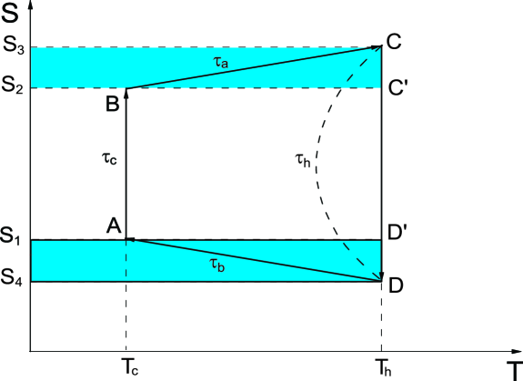
Figure 1: (Color online) Schematic diagram of an irreversible Carnot-like refrigeration cycle in the plane of the temperature $T$ and entropy $S$. The values of the entropy $S$ at the four special instants are indicated by $S_{i}$ ($i=1,3,3,4$). Here $\tau_{h,~{}c}$ are the times spent on the two isothermal process, while $\tau_{a,~{}b}$ represent the times taken for the two adiabatic processes. The blue area defined by the rectangles $C,C^{\prime},S_{2},S_{3}$ and $D,D^{\prime},S_{1},S_{4}$ represents the total work done by the system to overcome nonadiabatic dissipation in the two adiabatic processes.

An irreversible Carnot-like refrigeration cycle $A\rightarrow B\rightarrow C\rightarrow D\rightarrow A$ is drawn in the $(S,T)$ plane (see Fig. 1 ). During two isothermal processes $A\rightarrow B$ and $C\rightarrow D$, the working substance is in contact with a cold and a hot heat bath at constant temperatures $T_{h}$ and $T_{c}$, respectively. In the adiabatic process $B\rightarrow C$ ($D\rightarrow A$), the working substance is decoupled from the cold (hot) reservoir, and the entropy changes from $S_{B}$ to $S_{C}$ ($S_{D}$ to $S_{A}$). It can be seen from Fig. 1 that $S_{1}=S_{A}$, $S_{2}=S_{B}$, $S_{3}=S_{C}$ and $S_{4}=S_{D}$. For the reversible cycle where $S_{B}=S_{C}$ and $S_{A}=S_{D}$, we recover the Carnot efficient of performance $\varepsilon{{}_{C}}=\frac{T_{c}}{T_{h}-T_{c}}$, which is generically universal.

Now we turn to discussion on the Carnot-like cycle under finite-time operation that moves the working substance away from the equilibrium. In the isothermal process the system may be out of equilibrium, but it must be in the equilibrium with the heat reservoir at the special instants $i$ with $i=A,B,C,D$, at which the thermodynamic quantities of the system can be defined well. Unlike in the ideal case where any adiabatic process is isentropic, the adiabatic process is nonisentropic because of nonadiabatic dissipation. This dissipation develops additional heat and thus yields an increase in the entropy during the so-called adiabatic process. The irreversible Carnot-like refrigerator that consists of the two adiabatic and two isothermal processes is operated as follows (more details about the isothermal processes can be seen in Tu12 ).

1. Isothermal expansion $A\to B$. The working substance is in contact with the cold reservoir at temperature $T_{c}$ for a period $\tau_{c}$. In this expansion the constraint imposed on the system is loosened according to the external controlled parameter $\lambda_{c}(\tau)$ during the time interval $0<\tau<\tau_{c}$, where $\tau$ is the cycle-time variable. A certain amount of heat $Q_{c}$ is released to the cold reservoir and the variation of entropy can be expressed as

$$\Delta S_{c}=Q_{c}/T_{c}+\Delta S_{c}^{ir},$$ (1)

with $\Delta S_{c}^{ir}\geq 0$ being the irreversible entropy production.

2. Adiabatic compression $B\to C$. The entropy is increased due to irreversible entropy production caused by the nonadiabatic dissipation, while the constraint on the system is enhanced according to the external controlled parameter $\lambda_{a}(\tau)$ during the time interval $\tau_{c}<\tau<\tau_{c}+\tau_{a}$. The irreversible entropy production arising from the nonadiabatic dissipaton is denoted by

$$\Delta S_{a}^{ir}=S_{3}-S_{2}.$$ (2)

3. Isothermal compression $C\to D$. The working substance is coupled to a hot reservoir at constant temperature $T_{h}$ for time $\tau_{h}$. The constraint on the system is further enhanced with the external controlled parameter $\lambda_{h}(\tau)$ during the time interval $\tau_{c}+\tau_{a}<\tau<\tau_{c}+\tau_{a}+\tau_{h}$. Let $Q_{h}$ be an amount of heat released to the hot reservoir, we have the entropy variation,

$$\Delta S_{h}=-Q_{h}/T_{h}+\Delta S_{h}^{ir},$$ (3)

where $\Delta S_{h}^{ir}\geq 0$ is the irreversible entropy production.

4. Adiabatic expansion $D\to A$. Similar to the adiabatic compression, the working substance is decoupled from the hot reservoir. During this process, the controlled parameter $\lambda_{b}(\tau)$ changes from $\lambda_{b}(\tau_{c}+\tau_{a}+\tau_{h})$ to $\lambda_{b}(\tau_{c}+\tau_{a}+\tau_{h}+\tau_{b})$, so the constraint on the system is loosened. The entropy production due to the non-adiabatic dissipation reads

$$\Delta S_{b}^{ir}=S_{1}-S_{4}.$$ (4)

The system recovers to its initial state after a single cycle, and the total change of entropy of the system is vanishing for a whole cycle. That is, there exist a following relation:

$$\Delta S+\Delta S_{a}^{ir}+\Delta S_{h}+\Delta S_{b}^{ir}=0,$$ (5)

where we have defined $\Delta S\equiv\Delta S_{c}=S_{2}-S_{1}$.

Now we follow the low-dissipation assumption Esp10 that the irreversible entropy production during an isothermal process is assumed to be inversely proportional to the time required for completing this process, i.e., $\Delta S_{\kappa}^{ir}=\Sigma_{\kappa}/\tau_{\kappa}$, where $\Sigma_{\kappa}$ is a dissipation constant for the $\kappa$ process with $\kappa=a,b,c,h$ being the corresponding thermodynamic processes, respectively. As emphasized, the irreversible entropy production in any adiabatic process [$\Delta S_{a}^{ir}(\tau_{a})$ or $\Delta S_{b}^{ir}(\tau_{b})$] cannot be included by the irreversible entropy production in any isothermal process [$\Delta S_{c}^{ir}(\tau_{c})$ or $\Delta S_{h}^{ir}(\tau_{h})$], as lies in the fact that the irreversible entropy production $\Delta S_{\kappa}^{ir}(\tau_{\kappa})$ as a function of the time $\tau_{\kappa}$ depends on the time taken for the corresponding process $\kappa$. In contrast to the state variable $\Delta S$ that depends merely on the initial and final states of the isothermal processes, here $\Delta S_{\kappa}^{ir}$ are process variables depending on the detailed protocols. As for isothermal processes, we also adopt the low-dissipation assumption for any adiabatic process Fel00 ; Gor91 ; pre86 ; pre85 ; Rui13 to describe the irreversible entropy production. It is physically reasonable since the irreversible entropy production $\Delta S_{\kappa}^{ir}$ becomes much smaller and is vanishing in the longtime limit ($\tau_{\kappa}\rightarrow\infty)$ when the process is quasistatic.

Considering Eqs. (1), (2), (3), (4) and (5), the heat $Q_{c}$ and $Q_{h}$ are obtained,

$$Q_{c}=T_{c}\left({\Delta S-\Sigma_{c}/\tau_{c}}\right),$$ (6)

and

$$Q_{h}=T_{h}\left({\Delta S+\Sigma_{a}/\tau_{a}+\Sigma_{b}/\tau_{b}+\Sigma_{h}/\tau_{h}}\right).$$ (7)

As a consequence, the work consumed by the system per cycle ($W$) and the COP of the refrigeration cycle ($\varepsilon$), are derived as

$$W=Q_{h}-Q_{c}=\left({T_{h}-T_{c}}\right)\Delta S+T_{h}\Sigma_{h}/\tau_{h}+T_{c}\Sigma_{c}/\tau_{c}+T_{h}\left(\Sigma_{a}/\tau_{a}+\Sigma_{b}/\tau_{b}\right),$$ (8)

and

$$\varepsilon=\frac{Q_{c}}{Q_{h}-Q_{c}}=\frac{T_{c}\left({\Delta S-\Sigma_{c}/\tau_{c}}\right)}{\left({T_{h}-T_{c}}\right)\Delta S+T_{h}\left({\Sigma_{a}/\tau_{a}+\Sigma_{b}/\tau_{b}+\Sigma_{h}/\tau_{h}}\right)+T_{c}\Sigma_{c}/\tau_{c}}.$$ (9)

The last term in Eq. (8) represents the additional work consumed by the system because of the dissipation in the two adiabatic processes. This additional work to overcome the internally nonadiabatic dissipation is represented by the two blue areas in Fig. 1.

III Optimum analysis

In this section we present an optimum analysis of a refrigerator with internal dissipation which accounts for the irreversible entropy production during a nonisentropic adiabatic process (The more details about a nonisentropic adiabatic process can be found in Ref. pre86 ). If the adiabatic processes are assumed proceed instantaneously with constant entropy, we recall that Tom13 ; Tu12 : (i) the bounds of the COP under $\Omega$ criterion, between which there are small differences, are in agreement with the real experimental data within a range of temperatures of the working substance; (ii) under the $\chi$ criterion, the upper bound of the COP fits well with the experimental data, but the COP in the symmetric limit ($\varepsilon_{\chi}^{\Sigma_{h}=\Sigma_{c}}$) seems to be considerably larger than the experimental data. In what follows, our theoretical predictions are expected to agree well with the experimental data when compared with the experimental data. In particular, for the $\chi$ criterion, our theoretical data in the symmetric limit should match more closely with the experimental data than the ones obtained from the previous models without consideration of nonadiabatic dissipation Tom13 .

III.1 COP at $\chi$ figure of merit

Substitution of Eqs. (8) and (9) into the $\chi$ figure of merit as the target function, leads to

$$\chi=\frac{{\varepsilon{{Q_{c}}}}}{\tau}{=}\frac{{T_{c}^{2}\left({\Delta S-\Sigma_{c}x_{c}}\right)^{2}}}{{\left[{\left({T_{h}-T_{c}}\right)\Delta S+T_{h}\left({\Sigma_{a}x_{a}+\Sigma_{b}x_{b}+\Sigma_{h}x_{h}}\right){{+}}T_{c}\Sigma_{c}x_{c}}\right]\left({1/x_{a}+1/x_{b}+1/x_{c}+1/x_{h}}\right)}}.$$ (10)

Here and hereafter we adopt the variable transformation $x_{\kappa}=1/\tau_{\kappa}\left({\kappa=a,b,c,h}\right)$ by taking the inverse of time instead of the time itself as a variable.

We optimize the target function $\chi$ over the time variables $x_{\kappa}$ to specify the time spent on any thermodynamic process and also to maximize this figure of merit. Considering $\frac{{\partial\chi}}{{\partial x_{\kappa}}}=0\left({\kappa=a,b,c,h}\right)$, we find the four following relations:

$$\left({Q_{h}-Q_{c}}\right)x_{a}x_{b}x_{h}=T_{c}\Sigma_{c}x_{c}\left({2Q_{h}/Q_{c}-1}\right)\left({x_{a}x_{b}x_{c}+x_{a}x_{b}x_{h}+x_{b}x_{c}x_{h}+x_{a}x_{c}x_{h}}\right),$$ (11)

$$\left({Q_{h}-Q_{c}}\right)x_{b}x_{c}x_{h}=T_{h}\Sigma_{a}x_{a}\left({x_{a}x_{b}x_{c}+x_{a}x_{b}x_{h}+x_{b}x_{c}x_{h}+x_{a}x_{c}x_{h}}\right),$$ (12)

$$\left({Q_{h}-Q_{c}}\right)x_{a}x_{c}x_{h}=T_{h}\Sigma_{b}x_{b}\left({x_{a}x_{b}x_{c}+x_{a}x_{b}x_{h}+x_{b}x_{c}x_{h}+x_{a}x_{c}x_{h}}\right),$$ (13)

$$\left({Q_{h}-Q_{c}}\right)x_{a}x_{b}x_{c}=T_{h}\Sigma_{h}x_{h}\left({x_{a}x_{b}x_{c}+x_{a}x_{b}x_{h}+x_{b}x_{c}x_{h}+x_{a}x_{c}x_{h}}\right).$$ (14)

Dividing Eq. (11) by Eq. (12), Eq. (13), Eq. (14), respectively, we obtain,

$$\varepsilon^{*}_{\chi}T_{h}\Sigma_{a}x_{a}^{2}=\left({\varepsilon^{*}_{\chi}+2}\right)T_{c}\Sigma_{c}x_{c}^{2},$$ (15)

$$\varepsilon^{*}_{\chi}T_{h}\Sigma_{b}x_{b}^{2}=\left({\varepsilon^{*}_{\chi}+2}\right)T_{c}\Sigma_{c}x_{c}^{2},$$ (16)

$$\varepsilon^{*}_{\chi}T_{h}\Sigma_{h}x_{h}^{2}=\left({\varepsilon^{*}_{\chi}+2}\right)T_{c}\Sigma_{c}x_{c}^{2},$$ (17)

Here $\varepsilon^{*}_{\chi}$ is the COP under maximum $\chi$ condition. From Eqs. (15), (16), and (17), we find that the times spent on the four thermodynamic processes are optimally distributed as,

$$\tau_{\kappa}/\tau_{h}=\sqrt{\Sigma_{\kappa}/\Sigma_{h}}~{}(\kappa=a,b),\tau_{b}/\tau_{a}=\sqrt{\Sigma_{b}/\Sigma_{a}},$$ (18)

and

$$\tau_{\kappa}/\tau_{c}=\sqrt{T_{h}\Sigma_{\kappa}/(mT_{c}\Sigma_{c})}~{}\left({\kappa=a,b,h}\right),$$ (19)

where $m\equiv\sqrt{{(\varepsilon^{*}_{\chi}+2)}/\varepsilon^{*}_{\chi}}$ has been adopted and can be determined through numerical calculation of $\varepsilon_{\chi}^{*}$ [see Eqs. (20) and (24) discussed below]. Making summation over Eqs. (11), (12), (13), and (14), together with use of Eqs. (15), (16), and (17), we can derive after some simple reshuffling,

$$\frac{1}{{\varepsilon^{*}_{\chi}}}=\frac{1}{{\varepsilon_{C}}}+\frac{1}{{\varepsilon^{*}_{\chi}+\left[{\left({2\varepsilon_{C}-\varepsilon^{*}_{\chi}}\right)\alpha\left({1+\varepsilon_{C}}\right)}\right]}},$$ (20)

or

$$\varepsilon^{*}_{\chi}=\frac{{\varepsilon_{C}\left[{\sqrt{1+8\left({1+\varepsilon_{C}}\right)/\alpha}-3}\right]}}{{2\left[{\left({1+\varepsilon_{C}}\right)/\alpha-1}\right]}},$$ (21)

where we have used

$$\alpha\equiv\frac{{\Sigma_{c}x_{c}}}{{\Sigma_{a}x_{a}+\Sigma_{b}x_{b}+\Sigma_{c}x_{c}{\rm{+}}\Sigma_{h}x_{h}}}.$$ (22)

It is expected that this result will be reduced to the one based on idealized-adiabatic model in which $\Sigma_{a}=\Sigma_{b}=0$. The expression of $\alpha$ is derived from the more general model in which the nonadiabatic dissipation and the time spent on any adiabatic process are involved. Since $0\leq\alpha\leq 1$ and $\varepsilon_{C}>0$, $\varepsilon^{*}_{\chi}$ increases monotonously as $\alpha$, and vice versa. As a result, we re-derive the bounds of the COP at maximum $\chi$ figure of merit Tu12 ; Izu13 ,

$$0\equiv\varepsilon_{\chi}^{-}\leq\varepsilon^{*}_{\chi}\leq\varepsilon_{\chi}^{+}\equiv\left({\sqrt{9+8\varepsilon_{C}}-3}\right)/2.$$ (23)

It is thus clear that the inclusion of the nonadiabatic dissipation as well as the time taken for the adiabatic process does not change the upper and lower bounds of the COP at maximum $\chi$ figure of merit. These lower and upper bounds of $\varepsilon_{\chi}^{*}$ are achieved when $\alpha=0$, and $\alpha=1$, respectively. Combination of Eqs. (15), (16), (17), and (22) can eliminate the ratios $x_{\kappa}/x_{c}$ ($\kappa=h,a,b$), leading to

$$\alpha=\frac{1}{m\left(\sqrt{\frac{T_{c}\Sigma_{h}}{T_{h}\Sigma_{c}}}+\sqrt{\frac{T_{c}\Sigma_{a}}{T_{h}\Sigma_{c}}}+\sqrt{\frac{T_{c}\Sigma_{b}}{T_{h}\Sigma_{c}}}\right)+1},$$ (24)

with $m=\sqrt{{(\varepsilon^{*}_{\chi}+2)}/\varepsilon^{*}_{\chi}}$. The complete asymmetric limits $\Sigma_{c}/\Sigma_{\kappa}\rightarrow 0$ and $\Sigma_{c}/\Sigma_{\kappa}\rightarrow\infty$, where $\kappa$ represents $h,a,b$ but except $c$, cause the COP at maximum $\chi$ merit of figure to approach its upper and lower bounds, $\varepsilon_{\chi}^{-}=0$, and $\varepsilon_{\chi}^{+}=\left({\sqrt{9+8\varepsilon_{C}}-3}\right)/2$, respectively.

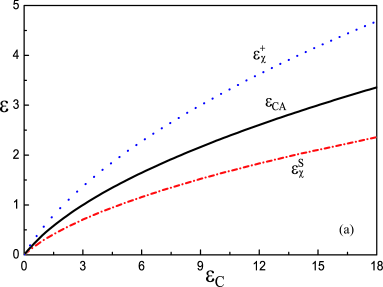
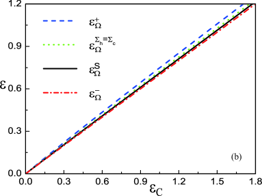
Figure 2: (Color online) (a)The values of $\varepsilon_{\chi}$ in the three limits, $\varepsilon_{\chi}^{+}$ (dotted blue line) , $\varepsilon_{CA}(=\varepsilon_{\chi}^{\Sigma_{h}=\Sigma_{c}})$ (black solid line), and $\varepsilon_{\chi}^{S}$ (red dot-dashed line), versus the Carnot COP $\varepsilon_{C}$; (b) The values of $\varepsilon_{\Omega}$ in the four cases, $\varepsilon_{\Omega}^{+}$ (blue dashed line), $\varepsilon_{\Omega}^{\Sigma_{h}=\Sigma_{c}}$ (green dotted line), $\varepsilon_{\Omega}^{S}$ (black solid line), and $\varepsilon_{\Omega}^{-}$ (red dot-dashed line), versus the Carnot COP $\varepsilon_{C}.$

When the dissipations in the two adiabatic and two isothermal processes are symmetric, respectively, we have $\Sigma_{a}=\Sigma_{b}=r\Sigma_{h}=r\Sigma_{c}$, with $r$ being the ratio. In such a case we consider three special situations: (i) $r\rightarrow 0$. The nonadiabatic dissipations for the two adiabatic processes are vanishing, while the dissipations during the two isothermal processes are symmetric. By using Eq. (21), the CA COP is recovered, $\varepsilon_{\chi}^{\Sigma_{h}=\Sigma_{c}}=\varepsilon_{CA}=\sqrt{1+\varepsilon_{C}}-1$, which is also the upper bound of the COP in such a case. (ii) $r\rightarrow\infty$. The lower bound of the COP is achieved, $\varepsilon_{\chi}^{-}=0$. (iii) $r=1$. The dissipations in four thermodynamic processes are symmetric. Here $\varepsilon_{\chi}^{S}\equiv\varepsilon_{\chi}(r=1)$ is defined for convenience, and its value can be done numerically based on Eqs. (20) and (24) for any given value of $T_{h}/T_{c}$ (i.e., the value of $\varepsilon_{C}$). At the super symmetric limit we obtain readily from Eqs. (18) and (19) that the time ratios of $\tau_{\kappa}/\tau_{c}$ $(\kappa=a,~{}b,~{}h)$ are $\tau_{\kappa}/\tau_{c}=\sqrt{T_{h}/(mT_{c})}$ with $m=\sqrt{{(\varepsilon^{*}_{\chi}+2)}/\varepsilon^{*}_{\chi}}$, and that the time allocations to the rest three processes are equal($\tau_{h}=\tau_{a}=\tau_{b})$. In Fig. 2 (a) we plot the COP $\varepsilon_{\chi}^{S}$ as a function of $\varepsilon_{C}$, comparing $\varepsilon_{CA}$ with the upper bound $\varepsilon_{\chi}^{+}$ of the Carnot-like refrigeration cycle.

III.2 COP at maximum ${\dot{\Omega}}$ figure of merit

The $\Omega$ criterion, a trade-off between maximum cooling and lost cooling loads, is defined as $\Omega=\left({2\varepsilon-\varepsilon_{\max}}\right){W}$ Her01 . The target function, $\dot{\Omega}=\left({2\varepsilon-\varepsilon_{\max}}\right)\frac{W}{\tau}$, can be expressed as

$$\dot{\Omega}=\left[{2Q_{c}-\varepsilon_{C}\left({Q_{h}-Q_{c}}\right)}\right]\left({x_{a}x_{b}x_{c}+x_{a}x_{b}x_{h}+x_{b}x_{c}x_{h}+x_{a}x_{c}x_{h}}\right)/x_{a}x_{b}x_{c}x_{h},$$ (25)

where we have made the variable transformation $x_{\kappa}=1/\tau_{\kappa}$ ($\kappa=h,c,a,b$). Setting the derivatives of $\dot{\Omega}$ with respect to $x_{\kappa}$ ($\kappa=h,c,a,b$) equal to zero, we derive the optimal equations:

$$\left[{2Q_{c}-\varepsilon_{C}\left({Q_{h}-Q_{c}}\right)}\right]\frac{{x_{b}x_{c}x_{h}}}{{x_{a}}}=T_{h}\Sigma_{a}\varepsilon_{C}\left({x_{a}x_{b}x_{c}+x_{a}x_{b}x_{h}+x_{b}x_{c}x_{h}+x_{a}x_{c}x_{h}}\right),$$ (26)

$$\left[{2Q_{c}-\varepsilon_{C}\left({Q_{h}-Q_{c}}\right)}\right]\frac{{x_{a}x_{c}x_{h}}}{{x_{b}}}=T_{h}\Sigma_{b}\varepsilon_{C}\left({x_{a}x_{b}x_{c}+x_{a}x_{b}x_{h}+x_{b}x_{c}x_{h}+x_{a}x_{c}x_{h}}\right),$$ (27)

$$\left[{2Q_{c}-\varepsilon_{C}\left({Q_{h}-Q_{c}}\right)}\right]\frac{{x_{a}x_{b}x_{c}}}{{x_{h}}}=T_{h}\Sigma_{h}\varepsilon_{C}\left({x_{a}x_{b}x_{c}+x_{a}x_{b}x_{h}+x_{b}x_{c}x_{h}+x_{a}x_{c}x_{h}}\right),$$ (28)

$$\left[{2Q_{c}-\varepsilon_{C}\left({Q_{h}-Q_{c}}\right)}\right]\frac{{x_{a}x_{b}x_{h}}}{{x_{c}}}=T_{c}\Sigma_{c}\left({2+\varepsilon_{C}}\right)\left({x_{a}x_{b}x_{c}+x_{a}x_{b}x_{h}+x_{b}x_{c}x_{h}+x_{a}x_{c}x_{h}}\right).$$ (29)

Dividing Eq. (29) by Eqs. (26), (27), and (28), respectively, we have

$$\frac{{x_{c}}}{{x_{a}}}=\sqrt{\frac{{\Sigma_{a}\left({1+\varepsilon_{C}}\right)}}{{\Sigma_{c}\left({2+\varepsilon_{C}}\right)}}},$$ (30)

$$\frac{{x_{c}}}{{x_{b}}}=\sqrt{\frac{{\Sigma_{b}\left({1+\varepsilon_{C}}\right)}}{{\Sigma_{c}\left({2+\varepsilon_{C}}\right)}}},$$ (31)

$$\frac{{x_{c}}}{{x_{h}}}=\sqrt{\frac{{\Sigma_{h}\left({1+\varepsilon_{C}}\right)}}{{\Sigma_{c}\left({2+\varepsilon_{C}}\right)}}}.$$ (32)

It follows, substitution of $\tau_{\kappa}=1/x_{\kappa}~{}(\kappa=h,c,a,b)$ into Eqs. (30), (31), and (32), that the optimal ratios of the time $\tau_{\kappa}/\tau_{h}~{}(\kappa=a,b)$ as well as $\tau_{b}/\tau_{a}$ are still given by Eq. (18), but that under the $\Omega$ criterion the time ratio $\tau_{\kappa}/\tau_{c}~{}(\kappa=h,a,b)$ becomes

$$\frac{\tau_{\kappa}}{\tau_{c}}=\sqrt{\frac{\Sigma_{\kappa}\left({1+\varepsilon_{C}}\right)}{\Sigma_{h}\left({2+\varepsilon_{C}}\right)}},\left({\kappa=a,b,h}\right).$$ (33)

Directly adding both sides of Eqs. (26), (27) (28), and (29), and using Eqs. (30), (31), and (32), leads to the result as

$$\Delta S=2\left({2+\varepsilon_{C}}\right)\Sigma_{c}x_{c}+2\left({1+\varepsilon_{C}}\right)\left({\Sigma_{a}x_{a}+\Sigma_{b}x_{b}+\Sigma_{h}x_{h}}\right).$$ (34)

It follows, substituting Eq. (34) into Eq. (9), that the COP at maximum $\dot{\Omega}$ conditions is

$$\varepsilon_{\Omega}^{*}=\frac{{3+2\varepsilon_{C}+2\gamma}}{{4+3\varepsilon_{C}+3\gamma}}\varepsilon_{C},$$ (35)

where $\gamma=\sqrt{\left({1+\varepsilon_{C}}\right)\left({2+\varepsilon_{C}}\right)\Sigma_{a}/\Sigma_{c}}+\sqrt{\left({1+\varepsilon_{C}}\right)\left({2+\varepsilon_{C}}\right)\Sigma_{b}/\Sigma_{c}}+\sqrt{\left({1+\varepsilon_{C}}\right)\left({2+\varepsilon_{C}}\right)\Sigma_{h}/\Sigma_{c}}$, which simplifies to $\gamma=\sqrt{\left({1+\varepsilon_{C}}\right)\left({2+\varepsilon_{C}}\right)\Sigma_{h}/\Sigma_{c}}$ in the ideal-adiabatic refrigeration cycle. The value of $\gamma$ is a non-negative number, varying from $0$ to $\infty$. Hence, the COP at maximum $\dot{\Omega}$ figure of merit, $\varepsilon_{\Omega}$, must be situated between

$$\varepsilon_{\Omega}^{-}\equiv\frac{2}{3}\varepsilon_{C}\leq\varepsilon_{\Omega}^{*}\leq\frac{{3+2\varepsilon_{C}}}{{4+3\varepsilon_{C}}}\varepsilon_{C}\equiv\varepsilon_{\Omega}^{+}.$$ (36)

The upper and lower bounds for the optimized COP at maximum $\dot{\Omega}$ figure of merit, $\varepsilon_{\Omega}^{-}$ and $\varepsilon_{\Omega}^{+}$, versus the Carnot COP $\varepsilon_{C}$, are plotted in Fig. 2(b).

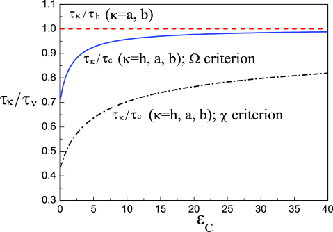
Figure 3: (Color online) The ratios of $\tau_{\kappa}/\tau_{\nu}$ ($\kappa=h,a,b$, and $\nu=h,c$) within maximum $\chi$ as well as $\dot{\Omega}$ figure of merit versus the Carnot COP $\varepsilon_{C}$ at the super symmetric limit. Here the optimal values of $\tau_{\kappa}/\tau_{c}$ ($\kappa=h,a,b$) under $\chi$ and $\Omega$ criteria, are indicated by a back dash-dotted a blue solid line, respectively. The values of $\tau_{\kappa}/\tau_{h}$ ($\kappa=a,b$) are equal to $1$ both under $\chi$ and $\Omega$ criteria, and are represented by a red dashed line.

As in the case of the $\chi$ figure of merit, the expression of COP at maximum $\dot{\Omega}$ condition similar to the corresponding one obtained in the model Tom13 with idealized adiabatic processes, and the internally nonadiabatic dissipation has no influence on the bounds of the COP. Here the optimal value of COP, however, represents a broader context by including the nonadiabatic dissipation and the time required for completing any adiabat. When adiabatic processes proceeds simultaneously and are isentropic ($\Sigma_{a}=\Sigma_{b}=0$), our result is reduced to that in Tom13 , as expected.

If the dissipations of the two adiabatic and two isothermal processes are symmetric, respectively, i.e., $\Sigma_{a}=\Sigma_{b}=r\Sigma_{c}=r\Sigma_{h}$, then $\gamma=(2\sqrt{r}+1)\sqrt{\left({1+\varepsilon_{C}}\right)\left({2+\varepsilon_{C}}\right)}$, and Eq. (35) becomes

$$\varepsilon_{\Omega}(r)=\frac{{3+2\varepsilon_{C}+\left({4\sqrt{r}+2}\right)\sqrt{\left({1+\varepsilon_{C}}\right)\left({2+\varepsilon_{C}}\right)}}}{{4+3\varepsilon_{C}+\left({6\sqrt{r}+3}\right)\sqrt{\left({1+\varepsilon_{C}}\right)\left({2+\varepsilon_{C}}\right)}}}\varepsilon_{C}.$$ (37)

From Eq. (37), we find in such a case that the bounds of the COP at maximum $\dot{\Omega}$ figure of merit are achieved, $\frac{2}{3}\varepsilon_{C}\leq\varepsilon_{\Omega}(r)\leq\frac{{3+2\varepsilon_{C}+2\sqrt{\left({1+\varepsilon_{C}}\right)\left({2+\varepsilon_{C}}\right)}}}{{4+3\varepsilon_{C}+3\sqrt{\left({1+\varepsilon_{C}}\right)\left({2+\varepsilon_{C}}\right)}}}\varepsilon_{C}$, when $r\rightarrow 0$ and $r\rightarrow\infty$, respectively. In the particular case when the dissipations of the four thermodynamic processes are symmetric, the COP can be obtained by the use of $r=1$,

$$\varepsilon^{S}_{\Omega}=\frac{{3+2\varepsilon_{C}+6\sqrt{\left({1+\varepsilon_{C}}\right)\left({2+\varepsilon_{C}}\right)}}}{{4+3\varepsilon_{C}+9\sqrt{\left({1+\varepsilon_{C}}\right)\left({2+\varepsilon_{C}}\right)}}}\varepsilon_{C}.$$ (38)

Then the optimal time ratios of $\tau_{\kappa}/\tau_{c}~{}(\kappa=h,a,b)$ in Eq. (33) simplifies to $\tau_{\kappa}/\tau_{c}=\sqrt{T_{c}/(2T_{h}-T_{c})}~{}(\kappa=h,a,b)$ in this super asymmetric case, while the optimized times spent on the other three processes are equal ($\tau_{a}=\tau_{b}=\tau_{h})$. At the super symmetric limit, the time ratios of $\tau_{\kappa}/\tau_{\nu}$, with $\kappa=h,a,b$ and $\nu=h,c$ as functions of the Carnot COP $\varepsilon_{C}$, under $\Omega$ and $\chi$ criteria, are plotted in Fig. 3 by using Eqs. (18), (19), and (33). Fig. 3 shows that, whether under $\chi$ or $\Omega$ criterion, the time taken for the cold isothermal process is larger than the ones for the other three processes, on which the times spent are equal to each other. This result is contrast to the fact that, for an irreversible heat engine pre86 , the hot isothermal process proceeds most slowly during a cycle, with equal times required for completing the cold isothermal and two adiabatic processes. This is not surprising, since the heat is transported into the system during the cold (hot) isothermal process for the refrigerator (heat engine), and the additional heat developed by the nonadiabatic dissipation is related to the high temperature $T_{h}$ (low temperature $T_{c}$) for the refrigerator (heat engine). For the model with idealized adiabatic processes ($\Sigma_{a}=\Sigma_{b}=0$), the symmetric limit ($r=1$) gives rise to the simple form of Eq. (35),

$$\varepsilon_{\Omega}^{\Sigma_{c}=\Sigma_{h}}\equiv\varepsilon_{\Omega}^{\Sigma_{h}=\Sigma_{c}}(\Sigma_{a}=\Sigma_{b}=0)=\frac{{\varepsilon_{C}}}{{\sqrt{\left({1+\varepsilon_{C}}\right)\left({2+\varepsilon_{C}}\right)}-\varepsilon_{C}}}.$$ (39)

At the symmetric limits (with and without nonadiabatic dissipation) the optimal COP’s, $\varepsilon_{\Omega}^{S}$ determined according to by Eqs. (38) and $\varepsilon_{\Omega}^{\Sigma_{c}=\Sigma_{h}}$ given by Eq. (39), are also shown in Fig. 2 (b). It is clear from Fig. 2 (b) that the nonadiabatic dissipation leads to a very slight decrease in the COP.

III.3 Comparison between our prediction with experimental data

It would be instructive to compare our theoretical predictions with the observed COP’s of some real refrigerators. Our theoretical prediction versus the data of the real refrigerators Gor00 at different values of temperature are plotted in Fig. 4, which shows that the theoretical results agree well with the experimental refrigerator data, whether at maximum $\chi$ or $\dot{\Omega}$ figure of merit. Applying the $\Omega$ criterion to optimization on the refrigerator cycle, we find that there are relatively small differences even between the lower and upper bounds ($\varepsilon_{\Omega}^{+}$ and $\varepsilon_{\Omega}^{-}$) of the COP for the refrigerator cycle. The values of COP, $\varepsilon_{\Omega}^{+},\varepsilon_{\Omega}^{\Sigma_{h}=\Sigma_{c}}$, $\varepsilon_{\Omega}^{S}$, and $\varepsilon_{\Omega}^{-}$ are indistinguishable in the plotted scale of Fig. 4 and are in good agreement with experimental data, particulary for some values of $\varepsilon_{C}$. Under maximum $\chi$ condition, our calculation of COP under maximum $\chi$ in the symmetric limit, $\varepsilon_{\chi}^{S}$, match more closely with the experimental data than the corresponding ones obtained in the previous model with idealized adiabatic processes, $\varepsilon_{CA}$=($\varepsilon_{\chi}^{\Sigma_{h}=\Sigma_{c}}$), as expected. Hence, our result suggests that internally nonadiabatic dissipation indeed induces the effects on the performance in the heat devices and thus can not be negligible in comparison with the experimental data.

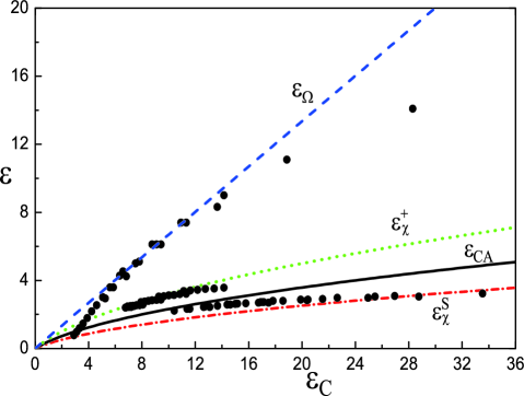
Figure 4: (Color online) Comparison between theoretical results (lines) and three sets of experimental results (points). Here $\varepsilon_{\Omega}$, $\varepsilon_{\chi}^{+}$, $\varepsilon_{CA}$, and $\varepsilon_{\chi}^{S}$, are indicated by a blue dashed line, a green dotted line,a black solid line, and a red dot-dashed line, respectively. The values in the four cases of $\varepsilon_{\Omega}$, $\varepsilon_{\Omega}^{+}$, $\varepsilon_{\Omega}^{\Sigma_{h}=\Sigma_{c}}$, $\varepsilon_{\Omega}^{S}$, and $\varepsilon_{\Omega}^{-}$, are indistinguishable and collapse into a single curve in this plotted scale.

IV conclusion

In conclusion, we have analyzed the COP at $\chi$ and $\dot{\Omega}$ figure of merits for an irreversible Carnot-like refrigerator with non-adiabatic dissipation. In the limits of extremely asymmetric dissipations, the COP either at maximum $\chi$ or at $\Omega$ figure of merit, converges to the same bounds as the corresponding ones obtained from previous models with idealized adiabatic processes. When the dissipations in two isothermal and two adiabatic processes are symmetric, respectively, comparison between our theoretical predictions of COP at maximum $\chi$ figure of merit and the observed COP’s of real refrigerators shows that our values matches more closely than the ones derived in previous models with no inclusion of non-adiabatic dissipation.

Acknowledgements: We gratefully acknowledge the financial support from the National Natural Science Foundation of China under Grant No. 11265010, No. 11065008, and No. 11191240252; the State Key Programs of China under Grant No. 2012CB921604; the Jiangxi Provincial Natural Science Foundation under Grant No. 20132BAB212009, China; and MICIN (Spain) under Grant No. FIS2010-17147FEDER. We are very grateful to Prof. Zhanchun Tu at Beijing Normal University for his valuable comments on the manuscript.

References

- (1) R. S. Berry, V. A. Kazakov, S. Sieniutycz, Z. Szwast, and A. M. Tsirlin, in Thermodynamics Optimization of Finite-Time Processes (John Wiley and Sons, Chichester, 2000).
- (2) C. Wu, L. Chen, and J. Chen, in Advances in Finite-Time Thermodynamics: Analysis and Optimization (Nova Science, New York, 2004).
- (3) A. Durmayaz, O. S. Sogut, B. Sahin, and H. Yavuz, Prog. Energy Combust. Sci. 30, 175 (2004).
- (4) C. Van den Broeck, Phys. Rev. Lett. 95, 190602 (2005).
- (5) Y. Izumida and K. Okuda, Europhys. Lett. 83, 60003 (2008); Phys. Rev. E 80, 021121 (2009).
- (6) M. Esposito, K.Lindenberg, and C. Van den Broeck, Phys. Rev. Lett. 102, 130602 (2009).
- (7) Z. C. Tu, J. Phys. A: Math. Theor. 41, 312003 (2008).
- (8) J. Guo, J. Wang, Y. Wang, and J. Chen, Phys. Rev. E 87, 012133 (2013).
- (9) X. L. Huang, L. C. Wang, and X. X. Yi, Phys. Rev. E 87, 012144 (2013).
- (10) Y. Wang and Z. C. Tu, Phys. Rev. E 85, 011127 (2012); Europhys. Lett. 98, 40001 (2012).
- (11) M. Esposito, R. Kawai, K. Lindenberg, and C. Van den Broeck, Phys. Rev. Lett. 105, 150603 (2010).
- (12) T. Schmiedl and U. Seifert, Europhys. Lett. 81, 20003 (2008).
- (13) U. Seifert, Phys. Rev. Lett. 106, 020601 (2011).
- (14) F. Curzon and B. Ahlborn, Am. J. Phys. 43, 22 (1975).
- (15) S. K. Ma, Stastical Mechanics (World Scientific, Singapore, 1985).
- (16) Z. Yan and J. Chen, J. Phys. D: Appl. Phys. 23, 136 (1990).
- (17) S. Velasco, J. M. M. Roco, and A. Calvo Hernández, Phys. Rev. Lett. 78, 3241 (1997).
- (18) A. E. Allahverdyan, K. Hovhannisyan, and G. Mahler, Phys. Rev. E 81, 051129 (2010).
- (19) C. de. Tomás, J. M .M.Roco, A. Calvo Hemández, Y. Wang, and Z. C. Tu, Phys. Rev. E 87, 012105 (2013).
- (20) C. de Tomás, A. Calvo Hernández, and J. M. M. Roco, Phys. Rev. E 85, 010104(R) (2012).
- (21) Y. Wang, M. Li, Z. C. Tu, A. Calvo Hernández, and J. M. M. Roco, Phys. Rev. E 86, 011127 (2012).
- (22) L. Chen, F. Sun, and W. Chen, Energy 20, 1049 (1995); L. Chen, F. Sun, C.Wu, and R. L. Kiang, Appl. Therm. Eng. 17, 401 (1997).
- (23) A. Calvo Hernández, A. Medina, J. M. M. Roco, J. A. White, and S. Velasco1, Phys. Rev. E 63, 037102 (2001).
- (24) N. Sánchez Salas and A. Calvo Hernández, Europhys. Lett. 61, 287 (2003); Phys. Rev. E 68, 046125 (2003).
- (25) B. Jiménez de Cisneros and A. Calvo Hernández, Phys. Rev. E 77, 041127 (2008).
- (26) N. Sánchez-Salas, L. López-Palacios, S. Velasco, and A. Calvo Hernández, Phys. Rev. E 82, 051101 (2010).
- (27) I. I. Novikov, J. Nucl. Energy 7, 125 (1958).
- (28) R. Wang, J. H. Wang, J. Z. He, and Y. L. Ma, Phys. Rev. E 87, 042119 (2013).
- (29) J. H. Wang and J. Z. He, Phys. Rev. E 86, 051112 (2012).
- (30) G. P. Beretta, Europhys. Lett. 99, 20005 (2012).
- (31) Y. Apertet, H. Ouerdane, C. Goupil, and Ph. Lecoeur, Phys. Rev. E 85, 041144 (2012).
- (32) J. H. Wang, J. Z. He, and Z. Q. Wu, Phys. Rev. E 85, 031145 (2012).
- (33) T. Feldmann and R. Kosloff, Phys. Rev. E 61, 4774 (2000); Y. Rezek and R. Kosloff, New J. Phys. 8, 83 (2006).
- (34) J. M. Gordon and M. Huleihil, J. Appl. Phys. 69, 1 (1991).
- (35) J. Chen, J. Phys. D: Appl. Phys. 27, 1144 (1994).
- (36) Y. Izumida, K. Okuda, A. Calvo Hernández, and J. M. M. Roco, Europhy. Lett. 101, 10005 (2013).
- (37) J. M. Gordon and C. N. Kim, Cool Thermodynamics (Cambridge International Science, Cornwall, UK, 2000).