Existence and conditional energetic stability of solitary gravity-capillary water waves with constant vorticity

Abstract

We present an existence and stability theory for gravity-capillary solitary waves with constant vorticity on the surface of a body of water of finite depth. Exploiting a rotational version of the classical variational principle, we prove the existence of a minimiser of the wave energy $\mathcal{H}$ subject to the constraint $\mathcal{I}=2\mu$, where $\mathcal{I}$ is the wave momentum and $0<\mu\ll 1$. Since $\mathcal{H}$ and $\mathcal{I}$ are both conserved quantities a standard argument asserts the stability of the set $D_{\mu}$ of minimisers: solutions starting near $D_{\mu}$ remain close to $D_{\mu}$ in a suitably defined energy space over their interval of existence.

In the applied mathematics literature solitary water waves of the present kind are described by solutions of a Korteweg-deVries equation (for strong surface tension) or a nonlinear Schrödinger equation (for weak surface tension). We show that the waves detected by our variational method converge (after an appropriate rescaling) to solutions of the appropriate model equation as $\mu\downarrow 0$.

1 Introduction

1.1 Variational formulation of the hydrodynamic problem

1.1.1 The water-wave problem

In this paper we consider a two-dimensional perfect fluid bounded below by a flat rigid bottom $\{y=0\}$ and above by a free surface $\{y=d+\eta(x,t)\}$. The fluid has unit density and flows under the influence of gravity and surface tension with constant vorticity $\omega$, so that the velocity field $(u(x,y,t),v(x,y,t))$ in the fluid domain $\Sigma_{\eta}=\{0<y<d+\eta(x,t)\}$ satisfies $v_{x}-u_{y}=\omega$. We study waves which are perturbations of underlying shear flows given by $\eta=0$ and $(u,v)=(\omega(d-y),0)$ (which may be a good description of tidal currents (see Constantin [Constantin, Chapter 2.3.2])) and are evanescent as $x\rightarrow\pm\infty$. In terms of a generalised velocity potential $\phi$ such that $(u,v)=(\phi_{x}+\omega(d-y),\phi_{y})$ and stream function $\psi$ such that $(u,v)=(\psi_{y},-\psi_{x})$, the governing equations are

$$\Delta\phi = \parbox{256.0748pt}{$0$,}0<y<d+\eta,$$

$$\phi_{y} = \parbox{256.0748pt}{$0$,}y=0,$$

$$\eta_{t} = \parbox{256.0748pt}{$\phi_{y}-\eta_{x}\phi_{x}+\omega\eta\eta_{x}$,}y=d+\eta,$$

$$\phi_{t} = \parbox{256.0748pt}{$\displaystyle-\frac{1}{2}|\nabla\psi|^{2}-\omega\psi-g\eta+\beta\left[\frac{\eta_{x}}{\sqrt{1+\eta_{x}^{2}}}\right]_{x}$,}y=d+\eta,$$

with $\eta(x,t)$, $\phi(x,y,t),\psi(x,y,t)+\frac{1}{2}\omega(d-y)^{2}\rightarrow 0$ as $x\rightarrow\pm\infty$, where $g$ and $\beta$ are respectively the acceleration due to gravity and the (positive) coefficient of surface tension (see Constantin, Ivanov & Prodanov [ConstantinIvanovProdanov08]).

At this point it is convenient to introduce dimensionless variables

$$(x^{\prime},y^{\prime})=\frac{1}{d}(x,y),\qquad t^{\prime}=\left(\frac{g}{d}\right)^{\!\frac{1}{2}}t,$$

$$\eta^{\prime}(x^{\prime},t^{\prime})=\frac{1}{d}\eta(x,t),\quad\phi^{\prime}(x^{\prime},t^{\prime})=\frac{1}{(gd^{3})^{\frac{1}{2}}}\phi(x,t),\quad\psi^{\prime}(x^{\prime},t^{\prime})=\frac{1}{(gd^{3})^{\frac{1}{2}}}\psi(x,t)$$

and parameters $\omega^{\prime}=\omega(d/g)^{\frac{1}{2}}$, $\beta^{\prime}=\beta/gd^{2}$; one obtains the equations

$$\Delta\phi = \parbox{256.0748pt}{$0$,}0<y<1+\eta,$$ (1)

$$\phi_{y} = \parbox{256.0748pt}{$0$,}y=0,$$ (2)

$$\eta_{t} = \parbox{256.0748pt}{$\phi_{y}-\eta_{x}\phi_{x}+\omega\eta\eta_{x}$,}y=1+\eta,$$ (3)

$$\phi_{t} = \parbox{256.0748pt}{$\displaystyle-\frac{1}{2}|\nabla\psi|^{2}-\omega\psi-\eta+\beta\left[\frac{\eta_{x}}{\sqrt{1+\eta_{x}^{2}}}\right]_{x}$,}y=1+\eta,$$ (4)

in which the primes have been dropped for notational simplicity. In particular we seek solitary-wave solutions of (1)–(4), that is waves of permanent form which propagate from right to left with constant (dimensionless) speed $\nu$, so that $\eta(x,t)=\eta(x+\nu t)$ (and of course $\eta(x+\nu t)\rightarrow 0$ as $x+\nu t\rightarrow\pm\infty$).

1.1.2 Formulation as a Hamiltonian system

We proceed by reducing the hydrodynamic problem to a pair of nonlocal, coupled evolutionary equations for the variables $\eta$ and $\xi=\phi|_{y=1+\eta}$. For fixed $\eta$ and $\xi$, let $\phi$ denote the unique solution to the boundary-value problem

$$\parbox{142.26378pt}{$\Delta\phi=0,$}0<y<1+\eta,$$

$$\parbox{142.26378pt}{$\phi=\xi,$}y=1+\eta,$$

$$\parbox{142.26378pt}{$\phi_{y}=0,$}y=0$$

and denote the harmonic conjugate of $\phi$ by $\tilde{\psi}$. We define the Hilbert transform $H(\eta)$ and Dirichlet-Neumann operator $G(\eta)$ for this boundary-value problem by

$$H(\eta)\xi=\tilde{\psi}|_{y=1+\eta},\qquad G(\eta)\xi=(\phi_{y}-\eta_{x}\phi_{x})|_{y=1+\eta},$$

so that $G(\eta)=-\partial_{x}H(\eta)$, and note that the boundary conditions (3), (4) can be written as

$$\eta_{t} = G(\eta)\xi+\omega\eta\eta_{x}$$ ,

$$\xi_{t} = -\frac{1}{2(1+\eta_{x}^{2})}\big{(}\xi_{x}^{2}-(G(\eta)\xi)^{2}-2\eta_{x}\xi_{x}G(\eta)\xi\big{)}$$

$$\qquad\mbox{}+\omega\eta\xi_{x}-\omega H(\eta)\xi-\eta+\beta\left[\frac{\eta_{x}}{\sqrt{1+\eta_{x}^{2}}}\right]_{x}$$.

Wahlén [Wahlen07] observed that the above equations can be formulated as the Hamiltonian system

$$\left(\begin{array}[]{c}\eta_{t}\\ \xi_{t}\end{array}\right)=\left(\begin{array}[]{cc}0&1\\ -1&\omega\partial_{x}^{-1}\end{array}\right)\!\!\left(\begin{array}[]{c}\delta_{\eta}\mathcal{H}\\ \delta_{\xi}\mathcal{H}\end{array}\right),$$ (5)

in which

$$\mathcal{H}(\eta,\xi)=\int_{-\infty}^{\infty}\left(\frac{\xi G(\eta)\xi}{2}+\omega\xi\eta\eta_{x}+\frac{\omega^{2}}{6}\eta^{3}+\frac{\eta^{2}}{2}+\beta(\sqrt{1+\eta_{x}^{2}}-1)\right)\,\mathrm{d}x,$$ (6)

(note that the well-known formulation of the water-wave problem by Zakharov [Zakharov68] is recovered in the irrotational case $\omega=0$). This Hamiltonian system has the conserved quantities $\mathcal{H}(\eta,\xi)$ (total energy) and

$$\mathcal{I}(\eta,\xi)=\int_{-\infty}^{\infty}\left(\xi\eta_{x}+\frac{\omega}{2}\eta^{2}\right)\,\mathrm{d}x,$$ (7)

(total horizontal momentum), which satisfies the equation

$$\left(\begin{array}[]{c}\eta_{x}\\ \xi_{x}\end{array}\right)=\left(\begin{array}[]{cc}0&1\\ -1&\omega\partial_{x}^{-1}\end{array}\right)\!\!\left(\begin{array}[]{c}\delta_{\eta}\mathcal{I}\\ \delta_{\xi}\mathcal{I}\end{array}\right);$$ (8)

these quantities are associated with its independence of respectively $t$ and $x$. According to (5) and (8), a solution of the form $\eta(x,t)=\eta(x+\nu t)$, $\xi(x,t)=\xi(x+\nu t)$ is characterised as a critical point of the total energy subject to the constraint of fixed momentum (cf. Benjamin [Benjamin84]). It is therefore a critical point of the functional $\mathcal{H}-\nu\mathcal{I}$, where the the speed of the wave is given by the Lagrange multiplier $\nu$. This functional depends on the single independent variable $x+\nu t$, which we now abbreviate to $x$.

A similar variational principle for waves of permanent form with a general distribution of vorticity has been used by Groves & Wahlén [GrovesWahlen07] in an existence theory for solitary waves. Groves & Wahlén interpreted their variational functional as an action functional and derived a formulation of the hydrodynamic problem as an infinite-dimensional spatial Hamiltonian system; a rich solution set is found using a centre-manifold reduction technique to convert it into a Hamiltonian system with a finite number of degrees of freedom.

In this paper we present a direct existence theory for minimisers of $\mathcal{H}$ subject to the constraint $\mathcal{I}=2\mu$ for $0<\mu<\mu_{0}$, where $\mu_{0}$ is a fixed positive constant chosen small enough for for the validity of our calculations. We seek constrained minimisers in a two-step approach.

1. Fix $\eta\neq 0$ and minimise $\mathcal{H}(\eta,\cdot)$ over $T_{\mu}=\{\xi:\mathcal{I}(\eta,\xi)=2\mu\}$. This problem (of minimising a quadratic functional over a linear manifold) admits a unique global minimiser $\xi_{\eta}$.

2. Minimise $\mathcal{J}_{\mu}(\eta):=\mathcal{H}(\eta,\xi_{\eta})$ over $\eta\in U\!\setminus\!\{0\}$, where $U$ is a fixed ball centred upon the origin in a suitable function space. Because $\xi_{\eta}$ minimises $\mathcal{H}(\eta,\cdot)$ over $T_{\mu}$ there exists a Lagrange multiplier $\nu_{\eta}$ such that

   $$G(\eta)\xi_{\eta}+\omega\eta\eta^{\prime}=\nu_{\eta}\eta^{\prime},$$

   and straightforward calculations show that

   $$\xi_{\eta}=\nu_{\eta}G(\eta)^{-1}\eta^{\prime}-\frac{\omega}{2}G(\eta)^{-1}(\eta^{2})_{x},$$

   $$\nu_{\eta}=\left(\frac{1}{2}\int_{-\infty}^{\infty}\eta^{\prime}G(\eta)^{-1}\eta^{\prime}\,\mathrm{d}x\right)^{\!\!-1}\!\!\left(\mu-\frac{\omega}{4}\int_{-\infty}^{\infty}\eta^{2}\,\mathrm{d}x+\frac{\omega}{4}\int_{-\infty}^{\infty}(\eta^{2})_{x}G(\eta)^{-1}\eta^{\prime}\,\mathrm{d}x\right),$$

   so that

   $$\mathcal{J}_{\mu}(\eta)=\mathcal{K}(\eta)+\frac{(\mu+\mathcal{G}(\eta))^{2}}{\mathcal{L}(\eta)},$$ (9)

   where

   $$\mathcal{G}(\eta) = \frac{\omega}{4}\int_{-\infty}^{\infty}\eta^{2}K(\eta)\eta\,\mathrm{d}x-\frac{\omega}{4}\int_{-\infty}^{\infty}\eta^{2}\,\mathrm{d}x,$$ (10)

   $$\mathcal{K}(\eta) = \int_{-\infty}^{\infty}\left(\frac{1}{2}\eta^{2}+\beta[\sqrt{1+\eta^{\prime 2}}-1]\right)\,\mathrm{d}x$$ (12)

   $$\qquad\quad\mbox{}-\frac{\omega^{2}}{2}\int_{-\infty}^{\infty}\frac{\eta^{2}}{2}K(\eta)\frac{\eta^{2}}{2}\,\mathrm{d}x+\frac{\omega^{2}}{6}\int_{-\infty}^{\infty}\eta^{3}\,\mathrm{d}x,\quad$$

   $$\mathcal{L}(\eta) = \frac{1}{2}\int_{-\infty}^{\infty}\eta K(\eta)\eta\,\mathrm{d}x$$ (13)

   and $K(\eta)=-\partial_{x}G(\eta)^{-1}\partial_{x}$. This computation also shows that the dimensionless speed of a solitary wave corresponding to a constrained minimiser $\eta$ of $\mathcal{H}$ is

   $$\nu=\frac{\mu+\mathcal{G}(\eta)}{\mathcal{L}(\eta)}.$$

This two-step approach to the constrained minimisation problem was introduced in a corresponding theory for irrotational solitary waves by Buffoni [Buffoni04a], who used a conformal mapping due to Babenko [Babenko87a, Babenko87b] to transform $\mathcal{J}_{\mu}$ into another functional $\tilde{\mathcal{J}}_{\mu}$ depending only upon $H(0)$ and hence simplify the necessary variational analysis. Buffoni established the existence of a (non-zero) minimiser of $\tilde{\mathcal{J}}_{\mu}$ for strong surface tension (Buffoni [Buffoni04a]) and obtained partial results in this direction for weak surface tension (Buffoni [Buffoni05, Buffoni09]). A method for completing his results for weak surface tension was sketched in a short note by Groves & Wahlén [GrovesWahlen10]; in the present paper we give complete details, including non-zero vorticity in our treatment and working directly with the original physical variables. Although versions of the Babenko transformation for non-zero constant vorticity have been published (Constantin & Varvaruca [ConstantinVarvaruca11], Martin [Martin13]), finding minimisers of $\mathcal{J}_{\mu}$ over $U\!\setminus\!\{0\}$ has the advantage of immediately yielding precise information on solutions to the original water-wave equations (1)–(4).

1.1.3 Functional-analytic framework

An appropriate functional-analytic framework for the above variational problem is introduced in Section 2. We work with the function spaces

$$H^{r}(\mathbb{R})=\overline{(\SS(\mathbb{R}),\|\cdot\|_{r})},\qquad\|\eta\|_{r}^{2}:=\int_{-\infty}^{\infty}(1+k^{2})^{r}|\hat{\eta}|^{2}\,\mathrm{d}k$$

for $r\in\mathbb{R}$ (the standard Sobolev spaces), and

$$H_{\star}^{1/2}(\mathbb{R})=\overline{(\SS(\mathbb{R}),\|\cdot\|_{H_{\star}^{1/2}(\mathbb{R})})},\qquad\|\eta\|_{H_{\star}^{1/2}(\mathbb{R})}^{2}:=\int_{-\infty}^{\infty}(1+k^{2})^{-\frac{1}{2}}k^{2}|\hat{\eta}|^{2}\,\mathrm{d}k,$$

$$H_{\star}^{-1/2}(\mathbb{R})=\overline{(\overline{\SS}(\mathbb{R}),\|\cdot\|_{H_{\star}^{-1/2}(\mathbb{R})})},\qquad\|\eta\|_{H_{\star}^{-1/2}(\mathbb{R})}^{2}:=\int_{-\infty}^{\infty}(1+k^{2})^{\frac{1}{2}}k^{-2}|\hat{\eta}|^{2}\,\mathrm{d}k;$$

here $\overline{(\SS(\mathbb{R}),\|\cdot\|)}$ denotes the completion of the inner product space constructed by equipping the Schwartz class $\SS(\mathbb{R})$ (or the subclass $\bar{\SS}(\mathbb{R})$ of Schwartz-class functions with zero mean) with the norm $\|\cdot\|$ and $\hat{\eta}=\mathcal{F}[\eta]$ is the Fourier transform of $\eta$.

The mathematical analysis of $G(\eta)$ and $K(\eta)$ is complicated by the fact that they are defined in terms of boundary-value problems in the variable domain $\Sigma_{\eta}$. Lannes [Lannes, Chapters 2 and 3] has presented a comprehensive theory for handling such such boundary-value problems by transforming them into serviceable nonlinear elliptic problems in the fixed domain $\Sigma_{0}$, and here we adapt Lannes’s methods to our specific requirements. Our main results are stated in the following theorem, according to which equations (10)–(13) define analytic functionals $\mathcal{G},\mathcal{K},\mathcal{L}:W^{s+3/2}\rightarrow\mathbb{R}$ for $s>0$. In accordance with this theorem we take $U=B_{M}(0)\subseteq H^{2}(\mathbb{R})$, where $M>0$ is chosen small enough so that $\overline{B}_{M}(0)\subseteq H^{2}(\mathbb{R})$ lies in $W^{s+3/2}$ and for for the validity of our calculations.

Theorem 1.1

Choose $h_{0}\in(0,1)$ and define $W=\{\eta\in W^{1,\infty}(\mathbb{R})\colon 1+\inf\eta>h_{0}\}$ and $W^{r}=H^{r}\cap W$ for $r\geq 0$.

• The Dirichlet-Neumann operator $G(\eta)$ is an isomorphism $H_{\star}^{1/2}(\mathbb{R})\to H_{\star}^{-1/2}(\mathbb{R})$ for each $\eta\in W$.

• The Dirichlet-Neumann operator $G(\cdot):W\rightarrow\mathcal{L}(H_{\star}^{1/2}(\mathbb{R}),H_{\star}^{-1/2}(\mathbb{R}))$ and Neumann-Dirichlet operator $G(\cdot)^{-1}:W\rightarrow\mathcal{L}(H_{\star}^{-1/2}(\mathbb{R}),H_{\star}^{1/2}(\mathbb{R}))$ are analytic.

• The operator $K(\cdot):W^{s+3/2}\rightarrow\mathcal{L}(H^{s+3/2}(\mathbb{R}),H^{s+1/2}(\mathbb{R}))$ is analytic for each $s>0$.

1.2 Heuristics

The existence of small-amplitude solitary waves is predicted by studying the dispersion relation for the linearised version of (1)–(4). Linear waves of the form $\eta(x,t)=\cos k(x+\nu t)$ exist whenever

$$1+\beta k^{2}-\omega\nu-\nu^{2}f(k)=0,\qquad f(k)=|k|\coth|k|,$$

that is whenever

$$\nu=-\frac{\omega}{2f(k)}+\frac{1}{2}\left(\frac{\omega^{2}}{f(k)^{2}}+\frac{4(1+\beta k^{2})}{f(k)}\right)^{\!\!\frac{1}{2}}.$$

The function $k\mapsto\nu(k)$, $k\geq 0$ has a unique global minimum $\nu_{0}=\nu(k_{0})$, and one finds that $k_{0}>0$ for $\beta<\beta_{\mathrm{c}}$ and $k_{0}=0$ (with $\nu_{0}=\nu(0)=\frac{1}{2}(-\omega+\sqrt{\omega^{2}+4})$) for $\beta>\beta_{\mathrm{c}}$, where

$$\beta_{\mathrm{c}}={\textstyle\frac{1}{6}}(\omega^{2}+2-\omega\sqrt{\omega^{2}+4})$$

(see Figure 1). For later use let us also note that

$$g(k):=1+\beta k^{2}-\omega\nu_{0}-\nu_{0}^{2}f(k)\geq 0,\qquad k\in\mathbb{R},$$

with equality precisely when $k=\pm k_{0}$.

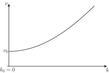
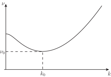
$\beta>\beta_{\mathrm{c}}\hskip 184.9429pt\beta<\beta_{\mathrm{c}}$

Figure 1: Dispersion relation for linear water waves

Bifurcations of nonlinear solitary waves are are expected whenever the linear group and phase speeds are equal, so that $\nu^{\prime}(k)=0$ (see Dias & Kharif [DiasKharif99, §3]). We therefore expect the existence of small-amplitude solitary waves with speed near $\nu_{0}$; the waves bifurcate from laminar flow when $\beta>\beta_{\mathrm{c}}$ and from a linear periodic wave train with frequency $k_{0}\nu(k_{0})$ when $\beta<\beta_{\mathrm{c}}$. Model equations for both types of solution have been derived by Johnson [Johnson12, §§4–5].

$\beta>\beta_{\mathrm{c}}$: The appropriate model equation is the Korteweg-deVries equation

$$-2u_{T}-\left(\beta-\frac{\nu_{0}^{2}}{3}\right)u_{XXX}+(\omega^{2}+3)uu_{X}=0,$$ (14)

in which

$$\eta=\mu^{\frac{2}{3}}u(X,T)+O(\mu^{\frac{4}{3}}),\qquad X=\mu^{\frac{1}{3}}(x+\nu_{0}t),\quad T=2(\omega^{2}+4)^{-\frac{1}{2}}\mu^{\frac{2}{3}}t.$$

At this level of approximation a solution to (14) of the form $u(X,T)=\phi(X+\nu_{\mathrm{KdV}}T)$ with $\phi(X)\rightarrow 0$ as $X\rightarrow\pm\infty$ corresponds to a solitary water wave with speed

$$\nu=\nu_{0}+2(\omega^{2}+4)^{-\frac{1}{2}}\mu^{\frac{2}{3}}\nu_{\mathrm{KdV}}=-{\textstyle\frac{1}{2}}\omega+{\textstyle\frac{1}{2}}(\omega^{2}+4)^{1/2}+2(\omega^{2}+4)^{-\frac{1}{2}}\mu^{\frac{2}{3}}\nu_{\mathrm{KdV}}.$$

The following lemma gives a variational description of the set of such solutions; the corresponding solitary waves are sketched in Figure 2.

Lemma 1.2

• The set of solutions to the ordinary differential equation

  $$-\left(\beta-\frac{\nu_{0}^{2}}{3}\right)\phi^{\prime\prime}-2\nu_{\mathrm{KdV}}\phi+\frac{3}{2}\left(\frac{\omega^{2}}{3}+1\right)\phi^{2}=0$$

  satisfying $\phi(X)\rightarrow 0$ as $X\rightarrow\infty$ is $D_{\mathrm{KdV}}=\{\phi_{\mathrm{KdV}}(\cdot+y)\colon y\in\mathbb{R}\},$ where

  $$\nu_{\mathrm{KdV}} = -\frac{\displaystyle 2\left(\frac{3}{16}\right)^{\!\!\frac{2}{3}}\left(\frac{\omega^{2}}{3}+1\right)^{\!\!\frac{4}{3}}}{\displaystyle\left(\beta-\frac{\nu_{0}^{2}}{3}\right)^{\!\!\frac{1}{3}}(\omega^{2}+4)^{\frac{1}{3}}},$$

  $$\phi_{\mathrm{KdV}}(x) = -\frac{\displaystyle\sqrt{3}\left(\frac{3}{16}\right)^{\!\!\frac{1}{6}}\left(\frac{\omega^{2}}{3}+1\right)^{\!\!\frac{1}{3}}}{\displaystyle\left(\beta-\frac{\nu_{0}^{2}}{3}\right)^{\!\!\frac{1}{3}}(\omega^{2}+4)^{\frac{1}{3}}}\operatorname{sech}^{2}\left(\frac{\displaystyle\left(\frac{3}{16}\right)^{\!\!\frac{1}{3}}\left(\frac{\omega^{2}}{3}+1\right)^{\!\!\frac{2}{3}}x}{\displaystyle\left(\beta-\frac{\nu_{0}^{2}}{3}\right)^{\!\!\frac{2}{3}}(\omega^{2}+4)^{\frac{1}{6}}}\right).$$

  These functions are precisely the minimisers of the functional $\mathcal{E}_{\mathrm{KdV}}:H^{1}(\mathbb{R})\rightarrow\mathbb{R}$ given by

  $$\mathcal{E}_{\mathrm{KdV}}(\phi)=\frac{1}{2}\int_{-\infty}^{\infty}\left(\left(\beta-\frac{\nu_{0}^{2}}{3}\right)(\phi^{\prime})^{2}+\left(\frac{\omega^{2}}{3}+1\right)\phi^{3}\right)\,\mathrm{d}x$$

  over the set $N_{\mathrm{KdV}}=\{\phi\in H^{1}(\mathbb{R}):\|\phi\|_{0}^{2}=2\alpha_{\mathrm{KdV}}\}$; the constant $2\nu_{\mathrm{KdV}}$ is the Lagrange multiplier in this constrained variational principle and

  $$c_{\mathrm{KdV}}:=\inf\left\{\mathcal{E}_{\mathrm{KdV}}(\phi)\colon\phi\in N_{\mathrm{KdV}}\right\}=-\frac{\displaystyle\frac{9}{5}\left(\frac{2}{3}\right)^{\!\!\frac{1}{3}}\left(\frac{\omega^{2}}{3}+1\right)^{\!\!\frac{4}{3}}}{\displaystyle\left(\beta-\frac{\nu_{0}^{2}}{3}\right)^{\!\!\frac{1}{3}}(\omega^{2}+4)^{\frac{5}{6}}}.$$

  Here the numerical value $\alpha_{\mathrm{KdV}}=2(\omega^{2}+4)^{-\frac{1}{2}}$ is chosen for compatibility with an estimate (Proposition 5.4) in the following water-wave theory.

• Suppose that $\{\phi_{m}\}\subset N_{\mathrm{KdV}}$ is a minimising sequence for $\mathcal{E}_{\mathrm{KdV}}$. There exists a sequence $\{x_{m}\}$ of real numbers with the property that a subsequence of $\{\phi_{m}(\cdot+x_{m})\}$ converges in $H^{1}(\mathbb{R})$ to an element of $D_{\mathrm{KdV}}$.

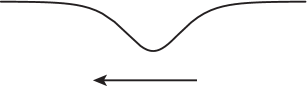
Figure 2: Korteweg-deVries theory predicts the existence of small-amplitude solitary waves of depression for strong surface tension

$\beta<\beta_{\mathrm{c}}$: The appropriate model equation is the cubic nonlinear Schrödinger equation

$$2\mathrm{i}A_{T}-\frac{1}{4}g^{\prime\prime}(k_{0})A_{XX}+\frac{3}{2}\left(\frac{A_{3}}{2}+A_{4}\right)|A|^{2}A=0,$$ (15)

in which

$$\eta=\frac{1}{2}\mu(A(X,T)\mathrm{e}^{\mathrm{i}k_{0}(x+\nu_{0}t)}+\mathrm{c.c.})+O(\mu^{2}),$$

$$X=\mu(x+\nu_{0}t),\qquad T=4k_{0}(\omega+2\nu_{0}f(k_{0}))^{-1}\mu^{2}t$$

and $A_{3}$, $A_{4}$ are functions of $\beta$ and $\omega$ which are given in Corollary 4.25 and Proposition 4.28 below; the abbreviation ‘$\mathrm{c.c.}$’ denotes the complex conjugate of the preceding quantity. (It is demonstrated in Appendix B that $A_{3}+2A_{4}$ is negative.) At this level of approximation a solution to (15) of the form $A(X,T)=\mathrm{e}^{\mathrm{i}\nu_{\mathrm{NLS}}T}\phi(X)$ with $\phi(X)\rightarrow 0$ as $X\rightarrow\pm\infty$ corresponds to a solitary water wave with speed

$$\nu=\nu_{0}+4(\omega+2\nu_{0}f(k_{0}))^{-1}\mu^{2}\nu_{\mathrm{NLS}}.$$

The following lemma gives a variational description of the set of such solutions (see Cazenave [Cazenave, §8]); the corresponding solitary waves are sketched in Figure 3.

Lemma 1.3

• The set of complex-valued solutions to the ordinary differential equation

  $$-\frac{1}{4}g^{\prime\prime}(k_{0})\phi^{\prime\prime}-2\nu_{\mathrm{NLS}}\phi+\frac{3}{2}\left(\frac{A_{3}}{2}+A_{4}\right)|\phi|^{2}\phi=0$$

  satisfying $\phi(X)\rightarrow 0$ as $X\rightarrow\infty$ is $D_{\mathrm{NLS}}=\{\mathrm{e}^{\mathrm{i}\omega}\phi_{\mathrm{NLS}}(\cdot+y)\colon\omega\in[0,2\pi),y\in\mathbb{R}\},$ where

  $$\nu_{\mathrm{NLS}} = -\frac{9\alpha_{\mathrm{NLS}}^{2}}{8g^{\prime\prime}(k_{0})}\left(\frac{A_{3}}{2}+A_{4}\right)^{\!\!2},$$

  $$\phi_{\mathrm{NLS}}(x) = \alpha_{\mathrm{NLS}}\left(-\frac{3}{g^{\prime\prime}(k_{0})}\left(\frac{A_{3}}{2}+A_{4}\right)\right)^{\!\!\frac{1}{2}}\operatorname{sech}\left(-\frac{3\alpha_{\mathrm{NLS}}}{g^{\prime\prime}(k_{0})}\left(\frac{A_{3}}{2}+A_{4}\right)x\right)$$

  These functions are precisely the minimisers of the functional $\mathcal{E}_{\mathrm{NLS}}:H^{1}(\mathbb{R})\rightarrow\mathbb{R}$ given by

  $$\mathcal{E}_{\mathrm{NLS}}(\phi)=\int_{-\infty}^{\infty}\left(\frac{1}{8}g^{\prime\prime}(k_{0})|\phi^{\prime}|^{2}+\frac{3}{8}\left(\frac{A_{3}}{2}+A_{4}\right)|\phi|^{4}\right)\,\mathrm{d}x$$

  over the set $N_{\mathrm{NLS}}=\{\phi\in H^{1}(\mathbb{R}):\|\phi\|_{0}^{2}=2\alpha_{\mathrm{NLS}}\}$; the constant $2\nu_{\mathrm{NLS}}$ is the Lagrange multiplier in this constrained variational principle and

  $$c_{\mathrm{NLS}}:=\inf\left\{\mathcal{E}_{\mathrm{NLS}}(\phi)\colon\phi\in N_{\mathrm{NLS}}\right\}=-\frac{3\alpha_{\mathrm{NLS}}^{3}}{4g^{\prime\prime}(k_{0})}\left(\frac{A_{3}}{2}+A_{4}\right)^{\!\!2}.$$

  Here the numerical value $\alpha_{\mathrm{NLS}}=\frac{1}{2}\left(\frac{1}{4}\nu_{0}f(k_{0})+\frac{\omega}{8}\right)^{-1}$ is chosen for compatibility with an estimate (Proposition 5.10) in the following water-wave theory.

• Suppose that $\{\phi_{n}\}\subset N_{\mathrm{NLS}}$ is a minimising sequence for $\mathcal{E}_{\mathrm{NLS}}$. There exists a sequence $\{x_{m}\}$ of real numbers with the property that a subsequence of $\{\phi_{m}(\cdot+x_{m})\}$ converges in $H^{1}(\mathbb{R})$ to an element of $D_{\mathrm{NLS}}$.

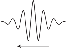
Figure 3: Nonlinear Schrödinger theory predicts the existence of small-amplitude envelope solitary waves for weak surface tension

1.3 The main results

In this paper we establish the existence of minimisers of the functional $\mathcal{J}_{\mu}$ over $U\!\setminus\!\{0\}$ and confirm that the corresponding solitary water waves are approximated by suitable scalings of the functions $\phi_{\mathrm{KdV}}$ (for $\beta>\beta_{\mathrm{c}}$) and $\phi_{\mathrm{NLS}}$ (for $\beta<\beta_{\mathrm{c}}$). The following theorem states these results more precisely.

Theorem 1.4

• The set $B_{\mu}$ of minimisers of $\mathcal{J}_{\mu}$ over $U\!\setminus\!\{0\}$ is non-empty.

• Suppose that $\{\eta_{m}\}$ is a minimising sequence for $\mathcal{J}_{\mu}$ on $U\!\setminus\!\{0\}$ which satisfies

  $$\sup_{m\in{\mathbb{N}}}\|\eta_{m}\|_{2}<M.$$

  There exists a sequence $\{x_{m}\}\subset\mathbb{R}$ with the property that a subsequence of $\{\eta_{m}(x_{m}+\cdot)\}$ converges in $H^{r}(\mathbb{R})$, $r\in[0,2)$, to a function $\eta\in B_{\mu}$.

• Suppose that $\beta>\beta_{\mathrm{c}}$. The set $B_{\mu}$ of minimisers of $\mathcal{J}_{\mu}$ over $U\!\setminus\!\{0\}$ satisfies

  $$\sup_{\eta\in B_{\mu}}\inf_{x\in\mathbb{R}}\|\phi_{\eta}-\phi_{\mathrm{KdV}}(\cdot+x)\|_{1}\rightarrow 0$$

  as $\mu\downarrow 0$, where we write

  $$\eta_{1}(x)=\mu^{\frac{2}{3}}\phi_{\eta}(\mu^{\frac{1}{3}}x)$$

  and $\eta_{1}$ is obtained from $\eta$ by multiplying its Fourier transform by the characteristic function of the interval $[-\delta_{0},\delta_{0}]$ with $\delta_{0}>0$. Furthermore, the speed $\nu_{\mu}$ of the corresponding solitary water waves satisfies

  $$\nu_{\mu}=\nu_{0}+2(\omega^{2}+4)^{-\frac{1}{2}}\nu_{\mathrm{KdV}}\mu^{\frac{2}{3}}+o(\mu^{\frac{2}{3}})$$

  uniformly over $\eta\in B_{\mu}$.

• Suppose that $\beta<\beta_{\mathrm{c}}$. The set $B_{\mu}$ of minimisers of $\mathcal{J}_{\mu}$ over $U\!\setminus\!\{0\}$ satisfies

  $$\sup_{\eta\in B_{\mu}}\inf_{\begin{subarray}{c}\omega\in[0,2\pi],\\ x\in\mathbb{R}\end{subarray}}\|\phi_{\eta}-e^{\mathrm{i}\omega}\phi_{\mathrm{NLS}}(\cdot+x)\|_{1}\rightarrow 0$$

  as $\mu\downarrow 0$, where we write

  $$\eta_{1}^{+}(x)=\frac{1}{2}\mu\phi_{\eta}(\mu x)\mathrm{e}^{\mathrm{i}k_{0}x},$$

  and $\eta_{1}^{+}$ is obtained from $\eta$ by multiplying its Fourier transform by the characteristic function of the interval $[k_{0}-\delta_{0},k_{0}+\delta_{0}]$ with $\delta_{0}\in(0,k_{0}/3)$. Furthermore, the speed $\nu_{\mu}$ of the corresponding solitary water waves satisfies

  $$\nu_{\mu}=\nu_{0}+4(\omega+2\nu_{0}f(k_{0}))^{-1}\nu_{\mathrm{NLS}}\mu^{2}+o(\mu^{2})$$

  uniformly over $\eta\in B_{\mu}$.

The first part of Theorem 1.4 is proved by reducing it to a special case of the second. We proceed by introducing the coercive penalised functional $\mathcal{J}_{\rho,\mu}:H^{2}(\mathbb{R})\rightarrow\mathbb{R}\cup\{\infty\}$ defined by

$$\mathcal{J}_{\rho,\mu}(\eta)=\left\{\begin{array}[]{lll}\displaystyle\mathcal{K}(\eta)+\frac{(\mu+\mathcal{G}(\eta))^{2}}{\mathcal{L}(\eta)}+\rho(\|\eta\|_{2}^{2}),&&\eta\in U\!\setminus\!\{0\},\\ \\ \infty,&&\eta\not\in U\!\setminus\!\{0\},\end{array}\right.$$

where $\rho:[0,M^{2})\rightarrow{\mathbb{R}}$ is a smooth, increasing ‘penalisation’ function which explodes to infinity as $t\uparrow M^{2}$ and vanishes for $0\leq t\leq\tilde{M}^{2}$; the number $\tilde{M}$ is chosen very close to $M$. Minimising sequences $\{\eta_{m}\}$ for $\mathcal{J}_{\rho,\mu}$, which clearly satisfy $\sup_{m\in{\mathbb{N}}}\|\eta_{m}\|_{2}<M$, are studied in detail in Section 3 with the help of the concentration-compactness principle (Lions [Lions84a, Lions84b]). The main difficulty here lies in discussing the consequences of ‘dichotomy’.

On the one hand the functionals $\mathcal{G}$, $\mathcal{K}$ and $\mathcal{L}$ are nonlocal and therefore do not act linearly when applied to the sum of two functions with disjoint supports. They are however ‘pseudolocal’ in the sense that

$$\begin{Bmatrix}\mathcal{G}\\ \mathcal{K}\\ \mathcal{L}\end{Bmatrix}(\eta_{m}^{(1)}+\eta_{m}^{(2)})-\begin{Bmatrix}\mathcal{G}\\ \mathcal{K}\\ \mathcal{L}\end{Bmatrix}(\eta_{m}^{(1)})-\begin{Bmatrix}\mathcal{G}\\ \mathcal{K}\\ \mathcal{L}\end{Bmatrix}(\eta_{m}^{(2)})\rightarrow 0$$

as $m\rightarrow\infty$, where $\{\eta_{m}^{(1)}\}$, $\{\eta_{m}^{(2)}\}$ have the properties that $\operatorname{supp}\eta_{m}^{(1)}\subset[-R_{m},R_{m}]$ and $\operatorname{supp}\eta_{m}^{(2)}\subset\mathbb{R}\!\setminus\!(-S_{m},S_{m})$ for sequences $\{R_{m}\}$, $\{S_{m}\}$ of positive real numbers with $R_{m}$, $S_{m}\rightarrow\infty$, $R_{m}/S_{m}\rightarrow 0$ as $m\rightarrow\infty$ (Lemma 3.9(iii)). This result is established in Section 2.2.2 by a new method which involves studying the weak formulation of the boundary-value problems defining the terms in the power-series expansion of $K$ about $\eta_{0}\in W^{s+3/2}$. On the other hand no a priori estimate is available to rule out ‘dichotomy’ at this stage; proceeding iteratively we find that minimising sequences can theoretically have profiles with infinitely many ‘bumps’. In particular we show that $\{\eta_{m}\}$ asymptotically lies in the region unaffected by the penalisation and construct a special minimising sequence $\{\tilde{\eta}_{m}\}$ for $\mathcal{J}_{\rho,\mu}$ which lies in a neighbourhood of the origin with radius $O(\mu^{\frac{1}{2}})$ in $H^{2}(\mathbb{R})$ and satisfies $\|\mathcal{J}^{\prime}_{\mu}(\tilde{\eta}_{m})\|_{0}\rightarrow 0$ as $n\rightarrow\infty$. The fact that the construction is independent of the choice of $\tilde{M}$ allows us to conclude that $\{\tilde{\eta}_{m}\}$ is also a minimising sequence for $\mathcal{J}_{\mu}$ over $U\!\setminus\!\{0\}$.

The special minimising sequence $\{\tilde{\eta}_{m}\}$ is used in Section 4 to establish the strict sub-additivity of the infimum $c_{\mu}$ of $\mathcal{J}_{\mu}$ over $U\!\setminus\!\{0\}$, that is the inequality

$$c_{\mu_{1}+\mu_{2}}<c_{\mu_{1}}+c_{\mu_{2}},\qquad 0<\mu_{1},\mu_{2},\mu_{1}+\mu_{2}<\mu_{0}.$$

The strict sub-additivity of $c_{\mu}$ follows from the fact that the function

$$a\mapsto a^{-q}\mathcal{M}_{a^{2}\mu}(a\tilde{\eta}_{m}),\qquad a\in[1,a_{0}],$$ (16)

is decreasing and strictly negative for some $q>2$ and $a_{0}\in(1,2]$, where

$$\mathcal{M}_{\mu}(\eta):=\mathcal{J}_{\mu}(\eta)-\mathcal{K}_{2}(\eta)-\frac{(\mu+\mathcal{G}_{2}(\eta))^{2}}{\mathcal{L}_{2}(\eta)}$$

is the ‘nonlinear’ part of $\mathcal{J}_{\mu}(\eta)$ (see Section 4.4). We proceed by approximating $\mathcal{M}_{\mu}(\eta_{m})$ with its dominant term and showing that this term has the required property.

The heuristic arguments given above suggest firstly that the spectrum of minimisers of $\mathcal{J}_{\mu}$ over $U\!\setminus\!\{0\}$ (that is, the support of their Fourier transform) is concentrated near wavenumbers $k=\pm k_{0}$, and secondly that they have the KdV or nonlinear Schrödinger length scales; the same should be true of the functions $\tilde{\eta}_{m}$, which approximate minimisers. We therefore decompose $\tilde{\eta}_{m}$ into the sum of a function $\tilde{\eta}_{m,1}$ whose spectrum is compactly supported near $k=\pm k_{0}$ and a function $\tilde{\eta}_{m,2}$ whose spectrum is bounded away from these points, and study $\tilde{\eta}_{m,1}$ using the weighted norm

$$|{\mskip-2.0mu}|{\mskip-2.0mu}|\eta|{\mskip-2.0mu}|{\mskip-2.0mu}|_{\alpha}^{2}:=\int_{-\infty}^{\infty}(1+\mu^{-4\alpha}(|k|-k_{0})^{4})|\hat{\eta}(k)|^{2}\,\mathrm{d}k.$$

A careful analysis of the equation $\mathcal{J}^{\prime}_{\mu}(\tilde{\eta}_{m})=O(\mu^{N})$ in $L^{2}(\mathbb{R})$ shows that $|{\mskip-2.0mu}|{\mskip-2.0mu}|\tilde{\eta}_{m,1}|{\mskip-2.0mu}|{\mskip-2.0mu}|_{\alpha}^{2}=O(\mu)$ and $\|\tilde{\eta}_{m,2}\|_{2}=O(\mu^{2+\alpha})$ for $\alpha<\frac{1}{3}$ when $\beta>\beta_{\mathrm{c}}$ and for $\alpha<1$ when $\beta<\beta_{\mathrm{c}}$. Using these estimates on the size of $\tilde{\eta}_{n}$, we find that

$$\mathcal{M}_{\mu}(\tilde{\eta}_{m})=\left\{\begin{array}[]{ll}\displaystyle c\!\!\int_{-\infty}^{\infty}\tilde{\eta}_{m,1}^{3}\,\mathrm{d}x+o(\mu^{\frac{5}{3}}),&\beta>\beta_{\mathrm{c}},\\ \\ \displaystyle-c\!\!\int_{-\infty}^{\infty}\tilde{\eta}_{m,1}^{4}\,\mathrm{d}x+o(\mu^{3}),\quad\mbox{}&\beta<\beta_{\mathrm{c}}.\end{array}\right.$$

That the function (16) is decreasing and strictly negative follows from the above estimate and the fact that $\mathcal{M}_{\mu}(\eta_{m})$ is negative for any minimising sequence $\{\eta_{m}\}$ for $\mathcal{J}_{\mu}$ over $U\!\setminus\!\{0\}$.

Knowledge of the strict sub-additivity property of $c_{\mu}$ (and general estimates for general minimising sequences) reduces the proof of part (ii) of Theorem 1.4 to a straightforward application of the concentration-compactness principle (see Section 5.1). Parts (iii) and (iv) are derived from Lemmata 1.2(ii) and 1.3(ii) by means of a scaling and contradiction argument from the estimates

$$\|\phi_{\eta}\|_{0}^{2}=2\begin{Bmatrix}\alpha_{\mathrm{KdV}}\\ \alpha_{\mathrm{NLS}}\end{Bmatrix}+o(1),\qquad\begin{Bmatrix}\mathcal{E}_{\mathrm{KdV}}\\ \mathcal{E}_{\mathrm{NLS}}\end{Bmatrix}(\phi_{\eta})=\begin{Bmatrix}c_{\mathrm{KdV}}\\ c_{\mathrm{NLS}}\end{Bmatrix}+o(1),\qquad\eta\in B_{\mu},$$

which emerge as part of the proof of Theorem 1.4(i) (see Section 5.2).

Some of the techniques used in the present paper were developed by Buffoni et al. [BuffoniGrovesSunWahlen13] in an existence theory for three-dimensional irrotational solitary waves. While we make reference to relevant parts of that paper, many aspects of our construction differ significantly from theirs. In particular, our treatment of nonlocal analytic operators is more comprehensive. Their version of Theorem 1.1 (see Lemmata 1.1 and 1.4 in that reference) is obtained using a less sophisticated ‘flattening’ transformation and shows only that the operators are analytic at the origin. Correspondingly, ‘pseudo-localness’ in the sense described above is established there only for constant-coefficient boundary-value problems (using an explcit representation of the solution by means of Green’s functions). Our treatment of the consequences of ‘dichotomy’ in the concentration-compactness principle (Section 3) is on the other hand similar to that given by Buffoni et al. [BuffoniGrovesSunWahlen13], and we omit proofs which are straightforward modifications of theirs; the main difference here is that negative values of the parameter $\mu$ emerge in our iterative construction of the special minimising sequence (see the remarks below Lemma 3.8).

1.4 Conditional energetic stability

Our original problem of finding minimisers of $\mathcal{H}(\eta,\xi)$ subject to the constraint $\mathcal{I}(\eta,\xi)=2\mu$ is also solved as a corollary to Theorem 1.4(ii); one follows the two-step minimisation procedure described in Section 1.1 (see Section 5.1).

Theorem 1.5

• The set $D_{\mu}$ of minimisers of $\mathcal{H}$ on the set

  $$S_{\mu}=\{(\eta,\xi)\in U\times H_{\star}^{1/2}(\mathbb{R}):\mathcal{I}(\eta,\xi)=2\mu\}$$

  is non-empty.

• Suppose that $\{(\eta_{m},\xi_{m})\}\subset S_{\mu}$ is a minimising sequence for $\mathcal{H}$ with the property that $\sup_{m\in\mathbb{N}}\|\eta_{m}\|_{2}<M$. There exists a sequence $\{x_{m}\}\subset\mathbb{R}$ with the property that a subsequence of $\{(\eta_{m}(x_{m}+\cdot),\xi_{m}(x_{m}+\cdot)\}$ converges in $H^{r}(\mathbb{R})\times H_{\star}^{1/2}(\mathbb{R})$, $r\in[0,2)$, to a function in $D_{\mu}$.

It is a general principle that the solution set of a constrained minimisation problem constitutes a stable set of solutions of the corresponding initial-value problem (e.g. see Cazenave & Lions [CazenaveLions82]). The usual informal interpretation of the statement that a set $X$ of solutions to an initial-value problem is ‘stable’ is that a solution which begins close to a solution in $X$ remains close to a solution in $X$ at all subsequent times. Implicit in this statement is the assumption that the initial-value problem is globally well-posed, that is every pair $(\eta_{0},\Phi_{0})$ in an appropriately chosen set is indeed the initial datum of a unique solution $t\mapsto(\eta(t),\Phi(t))$, $t\in[0,\infty)$. At present there is no global well-posedness theory for gravity-capillary water waves with constant vorticity (although there is a large and growing body of literature concerning well-posedness issues for water-wave problems in general). Assuming the existence of solutions, we obtain the following stability result as a corollary of Theorem 1.5 using the argument given by Buffoni et al. [BuffoniGrovesSunWahlen13, Theorem 5.5]. (The only property of a solution $(\eta,\xi)$ to the initial-value problem which is relevant to stability theory is that $\mathcal{H}(\eta(t),\xi(t))$ and $\mathcal{I}(\eta(t),\xi(t))$ are constant; we therefore adopt this property as the definition of a solution.)

Theorem 1.6

Suppose that $(\eta,\xi):[0,T]\rightarrow U\times H_{\star}^{1/2}(\mathbb{R})$ has the properties that

$$\mathcal{H}(\eta(t),\xi(t))=\mathcal{H}(\eta(0),\xi(0)),\ \mathcal{I}(\eta(t),\xi(t))=\mathcal{I}(\eta(0),\xi(0)),\qquad t\in[0,T]$$

and

$$\sup_{t\in[0,T]}\|\eta(t)\|_{2}<M.$$

Choose $r\in[0,2)$, and let ‘$\operatorname{dist}$’ denote the distance in $H^{r}(\mathbb{R})\times H_{\star}^{1/2}(\mathbb{R})$. For each $\varepsilon>0$ there exists $\delta>0$ such that

$$\operatorname{dist}((\eta(0),\xi(0)),D_{\mu})<\delta\quad\Rightarrow\quad\operatorname{dist}((\eta(t),\xi(t)),D_{\mu})<\varepsilon$$

for $t\in[0,T]$.

This result is a statement of the conditional, energetic stability of the set $D_{\mu}$. Here energetic refers to the fact that the distance in the statement of stability is measured in the ‘energy space’ $H^{r}(\mathbb{R})\times H_{\star}^{1/2}(\mathbb{R})$, while conditional alludes to the well-posedness issue. Note that the solution $t\mapsto(\eta(t),\xi(t))$ may exist in a smaller space over the interval $[0,T]$, at each instant of which it remains close (in energy space) to a solution in $D_{\mu}$. Furthermore, Theorem 1.6 is a statement of the stability of the set of constrained minimisers $D_{\mu}$; establishing the uniqueness of the constrained minimiser would imply that $D_{\mu}$ consists of translations of a single solution, so that the statement that $D_{\mu}$ is stable is equivalent to classical orbital stability of this unique solution (Benjamin [Benjamin74]). The phrase ‘conditional, energetic stability’ was introduced by Mielke [Mielke02] in his study of the stability of irrotational solitary water waves with strong surface tension using dynamical-systems methods.

2 The functional-analytic setting

2.1 Nonlocal operators

The goal of this section is to introduce rigorous definitions of the Dirichlet-Neumann operator $G(\eta)$, its inverse $N(\eta)$ and the operator $K(\eta):=-\partial_{x}(N(n)\partial_{x})$.

2.1.1 Function spaces

Choose $h_{0}\in(0,1)$. We consider the class

$$W=\{\eta\in W^{1,\infty}(\mathbb{R})\colon 1+\inf\eta>h_{0}\}$$

of surface profiles and denote the fluid domain by

$$\Sigma_{\eta}=\{(x,y)\in\mathbb{R}^{2}\colon 0<y<1+\eta(x)\},\qquad\eta\in W.$$

The observation that velocity potentials are unique only up to additive constants leads us to introduce the completion $H_{\star}^{1}(\Sigma_{\eta})$ of

$$\SS(\Sigma_{\eta})=\{\phi\in C^{\infty}(\overline{\Sigma}_{\eta}):|x|^{m}|\partial_{x}^{\alpha_{1}}\partial_{y}^{\alpha_{2}}\phi|\mbox{ is bounded for all }m,\alpha_{1},\alpha_{2}\in{\mathbb{N}}_{0}\}$$

with respect to the Dirichlet norm as an appropriate function space for $\phi$. The corresponding space for the trace $\phi|_{y=1+\eta}$ is the space $H_{\star}^{1/2}(\mathbb{R})$ defined in Section 1.1.3.

Proposition 2.1

Fix $\eta\in W$. The trace map $\phi\mapsto\phi|_{y=1+\eta}$ defines a continuous operator $H^{1}_{\star}(\Sigma_{\eta})\rightarrow H_{\star}^{1/2}(\mathbb{R})$ with a continuous right inverse $H_{\star}^{1/2}(\mathbb{R})\rightarrow H_{\star}^{1}(\Sigma_{\eta})$.

We also use anisotropic function spaces for functions defined in the strip $\Sigma_{0}=\mathbb{R}\times(0,1)$.

Definition 2.2

Suppose that $r\in\mathbb{R}$ and $n\in\mathbb{N}_{0}$.

• The Banach space $(L^{\infty}H^{r},\|\cdot\|_{r,\infty})$ is defined by

  $$L^{\infty}H^{r}=L^{\infty}((0,1),H^{r}(\mathbb{R})),\qquad\|u\|_{r,\infty}=\mathop{\operatorname{ess\,sup}}_{y\in(0,1)}\|u(\cdot,y)\|_{H^{r}(\mathbb{R})}.$$

• The Banach space $(H^{r,m},\|\cdot\|_{r,m})$ is defined by

  $$H^{r,m}=\bigcap_{j=0}^{n}H^{j}((0,1),H^{r-j}(\mathbb{R})),\qquad\|u\|_{r,m}=\sum_{j=0}^{n}\|\Lambda^{r-j}\partial_{y}^{j}u\|_{L^{2}(\Sigma)},$$

  where $\Lambda f=\mathcal{F}^{-1}[(1+k^{2})^{\frac{1}{2}}\hat{f}(k)]$.

The following propositions state some properties of these function spaces which are used in the subsequent analysis; they are deduced from results for standard Sobolev spaces (see Hörmander [Hoermander, Theorem 8.3.1] for Proposition 2.4).

Proposition 2.3

• The space $C_{0}^{\infty}(\overline{\Sigma})$ is dense in $H^{r,1}$ for each $r\in\mathbb{R}$.

• For each $r\in\mathbb{R}$ the mapping $u\mapsto u|_{y=1}$, $u\in C_{0}^{\infty}(\overline{\Sigma})$, extends continuously to an operator $H^{r+1,1}\rightarrow H^{r+1/2}(\mathbb{R})$.

• The space $H^{r+1,1}$ is continuously embedded in $L^{\infty}H^{r+1/2}$ for each $r\in\mathbb{R}$.

• The space $H^{r+1,1}$ is a Banach algebra for each $r>0$.

Proposition 2.4

Suppose that $r_{0}$, $r_{1}$, $r_{2}$ satisfy $r_{0}\leq r_{1}$, $r_{0}\leq r_{2}$, $r_{1}+r_{2}\geq 0$ and $r_{0}<r_{1}+r_{2}-\frac{1}{2}$. The product $u_{1}u_{2}$ of each $u_{1}\in L^{\infty}H^{r_{1}}$ and $u_{2}\in H^{r_{2},0}$ lies in $H^{r_{0},0}$ and satisfies

$$\|u_{1}u_{2}\|_{r_{0},0}\leq c\|u_{1}\|_{r_{1},\infty}\|u_{2}\|_{r_{2},0}.$$

Proposition 2.5

For each bounded linear function $L:L^{2}(\mathbb{R})\rightarrow L^{\infty}H^{0}$ the formula $(\eta,w)\mapsto L(\eta)w$ defines a bounded bilinear function $L^{2}(\mathbb{R})\times H^{1}(\Sigma)\rightarrow L^{2}(\Sigma)$ which satisfies the estimate

$$\|L(\eta)w\|_{0}\leq c\|L\|\|w\|_{0}^{\frac{1}{2}}\|w\|_{1}^{\frac{1}{2}}\|\eta\|_{0}.$$

The assertion remains valid when $\Sigma$ is replaced by $\{|x|<M\}$ or $\{|x|>M\}$ and the estimate holds uniformly over all values of $M$ greater than unity.

2.1.2 The Dirichlet-Neumann operator

The Dirichlet-Neumann operator $G(\eta)$ for the boundary-value problem

$$\parbox{170.71652pt}{$\Delta\phi=0,$}0<y<1+\eta,$$ (17)

$$\parbox{170.71652pt}{$\phi=\xi,$}y=1+\eta,$$ (18)

$$\parbox{170.71652pt}{$\phi_{y}=0,$}y=0$$ (19)

is defined formally as follows: fix $\xi=\xi(x)$, solve (17)–(19) and set

$$G(\eta)\xi=(\phi_{y}-\eta^{\prime}\phi_{x})|_{y=1+\eta}.$$

Our rigorous definition of $G(\eta)$ is given in terms of weak solutions to (17)–(19) (see Lannes [Lannes, Proposition 2.9] for the proof of Lemma 2.7).

Definition 2.6

Suppose that $\xi\in H_{\star}^{1/2}(\mathbb{R})$ and $\eta\in W$. A weak solution of (17)–(19) is a function $\phi\in H^{1}_{\star}(\Sigma_{\eta})$ with $\phi|_{y=1+\eta}=\xi$ which satisfies

$$\int_{\Sigma_{\eta}}\nabla\phi\cdot\nabla\psi\,\mathrm{d}x\,\mathrm{d}y=0$$

for all $\psi\in H^{1}_{\star}(\Sigma_{\eta})$ with $\psi|_{y=1+\eta}=0$.

Lemma 2.7

For each $\xi\in H_{\star}^{1/2}(\mathbb{R})$ and $\eta\in W$ there exists a unique weak solution $\phi$ of (17)–(19). The solution satisfies the estimate

$$\|\phi\|_{H_{\star}^{1}(\Sigma_{\eta})}\leq C\|\xi\|_{H_{\star}^{1/2}(\mathbb{R})},$$

where $C=C(\|\eta\|_{1,\infty})$.

Definition 2.8

Suppose that $\eta\in W$ and $\xi\in H_{\star}^{1/2}(\mathbb{R})$. The Dirichlet-Neumann operator is the bounded linear operator $G(\eta)\colon H_{\star}^{1/2}(\mathbb{R})\rightarrow H_{\star}^{-1/2}(\mathbb{R})$ defined by

$$\int_{-\infty}^{\infty}(G(\eta)\xi_{1})\,\xi_{2}\,\mathrm{d}x=\int_{\Sigma_{\eta}}\nabla\phi_{1}\cdot\nabla\phi_{2}\,\mathrm{d}x\,\mathrm{d}y,$$

where $\phi_{j}\in H^{1}_{\star}(\Sigma_{\eta})$ is the unique weak solution of (17)–(19) with $\xi=\xi_{j}$, $j=1,2$.

2.1.3 The Neumann-Dirichlet operator

The Neumann-Dirichlet operator $N(\eta)$ for the the boundary-value problem

$$\parbox{170.71652pt}{$\Delta\phi=0,$}0<y<1+\eta,$$ (20)

$$\parbox{170.71652pt}{$\phi_{y}-\eta^{\prime}\phi_{x}=\xi,$}y=1+\eta,$$ (21)

$$\parbox{170.71652pt}{$\phi_{y}=0,$}y=0$$ (22)

is defined formally as follows: fix $\xi=\xi(x)$, solve (20)–(22) and set

$$N(\eta)\xi=\phi|_{y=1+\eta}.$$

Our rigorous definition of $N(\eta)$ is also given in terms of weak solutions; Lemma 2.10 is proved in the same fashion as Lemma 2.7.

Definition 2.9

Suppose that $\xi\in H_{\star}^{-1/2}(\mathbb{R})$ and $\eta\in W$. A weak solution of (20)–(22) is a function $\phi\in H^{1}_{\star}(\Sigma_{\eta})$ which satisfies

$$\int_{\Sigma_{\eta}}\nabla\phi\cdot\nabla\psi\,\mathrm{d}x\,\mathrm{d}y=\int_{-\infty}^{\infty}\xi\psi|_{y=1+\eta}\,\mathrm{d}x$$

for all $\psi\in H^{1}_{\star}(\Sigma_{\eta})$.

Lemma 2.10

For each $\xi\in H_{\star}^{-1/2}(\mathbb{R})$ and $\eta\in W$ there exists a unique weak solution $\phi$ of (20)–(22). The solution satisfies the estimate

$$\|\phi\|_{H_{\star}^{1}(\Sigma_{\eta})}\leq C\|\xi\|_{H_{\star}^{-1/2}(\mathbb{R})},$$

where $C=C(\|\eta\|_{1,\infty})$.

Definition 2.11

Suppose that $\eta\in W$ and $\xi\in H_{\star}^{-1/2}(\mathbb{R})$. The Neumann-Dirichlet operator is the bounded linear operator $N(\eta)\colon H_{\star}^{-1/2}(\mathbb{R})\rightarrow H_{\star}^{1/2}(\mathbb{R})$ defined by

$$N(\eta)\xi=\phi|_{y=1+\eta},$$

where $\phi\in H^{1}_{\star}(\Sigma_{\eta})$ is the unique weak solution of (20)–(22).

The relationship between $G(\eta)$ and $N(\eta)$ is clarified by the following result, which follows from the definitions of these operators.

Lemma 2.12

Suppose that $\eta\in W$. The operator $G(\eta)\in\mathcal{L}(H_{\star}^{1/2}(\mathbb{R}),H_{\star}^{-1/2}(\mathbb{R}))$ is invertible with $G(\eta)^{-1}=N(\eta)$.

2.1.4 Analyticity of the operators

Let us begin by recalling the definition of analyticity given by Buffoni & Toland [BuffoniToland, Definition 4.3.1] together with a precise formulation of our result in their terminology.

Definition 2.13

Let $X$ and $Y$ be Banach spaces, $U$ be a non-empty, open subset of $X$ and $\mathcal{L}_{\mathrm{s}}^{k}(X,Y)$ be the space of bounded, $k$-linear symmetric operators $X^{k}\rightarrow Y$ with norm

$$|{\mskip-2.0mu}|{\mskip-2.0mu}|m|{\mskip-2.0mu}|{\mskip-2.0mu}|:=\inf\{c:\|m(\{f\}^{(k)})\|_{Y}\leq c\|f\|_{X}^{k}\mbox{ \rm{for all} }f\in X\}.$$

A function $F:U\rightarrow Y$ is analytic at a point $x_{0}\in U$ if there exist real numbers $\delta,r>0$ and a sequence $\{m_{k}\}$, where $m_{k}\in\mathcal{L}_{\mathrm{s}}^{k}(X,Y)$, $k=0,1,2,\ldots$, with the properties that

$$F(x)=\sum_{k=0}^{\infty}m_{k}(\{x-x_{0}\}^{(k)}),\qquad x\in B_{\delta}(x_{0})$$

and

$$\sup_{k\geq 0}r^{k}|{\mskip-2.0mu}|{\mskip-2.0mu}|m_{k}|{\mskip-2.0mu}|{\mskip-2.0mu}|<\infty.$$

The function is analytic if it is analytic at each point $x_{0}\in U$.

Theorem 2.14

• The Dirichlet-Neumann operator $G(\cdot):W\rightarrow\mathcal{L}(H_{\star}^{1/2}(\mathbb{R}),H_{\star}^{-1/2}(\mathbb{R}))$ is analytic.

• The Neumann-Dirichlet operator $N(\cdot):W\rightarrow\mathcal{L}(H_{\star}^{-1/2}(\mathbb{R}),H_{\star}^{1/2}(\mathbb{R}))$ is analytic.

To prove this theorem we study the dependence of solutions to the boundary-value problems (17)–(19) and (20)–(22) on $\eta$ by transforming them into equivalent problems in the fixed domain $\Sigma:=\Sigma_{0}$. For this purpose we define a change of variable $(x,y)=F^{\delta}(x,y^{\prime})$ in the following way. Choose $\delta>0$ and an even function $\chi\in C_{0}^{\infty}(\mathbb{R})$ with $\chi(k)\in[0,1]$ for $k\in\mathbb{R}$, $\operatorname{supp}\chi\in[-2,2]$ and $\chi(x)\equiv 1$ for $|x|\leq 1$, write

$$\eta^{\delta}(x,y^{\prime})=\mathcal{F}^{-1}[\chi(\delta(1-y^{\prime})k)\hat{\eta}(k)](x)$$

and define

$$F^{\delta}(x,y^{\prime})=(x,y^{\prime}(1+\eta^{\delta}(x,y^{\prime})))=(x,y^{\prime}+f^{\delta}(x,y^{\prime})),$$

in which $f^{\delta}(x,y^{\prime})=y^{\prime}\eta^{\delta}(x,y^{\prime})$.

Lemma 2.15

Suppose that $\eta\in W$. The mapping $F^{\delta}$ is a bijection $\Sigma\rightarrow\Sigma_{\eta}$ and $\overline{\Sigma}\rightarrow\overline{\Sigma}_{\eta}$ with $y\in C_{\mathrm{b}}^{1}(\Sigma)$, $y^{\prime}\in C_{\mathrm{b}}^{1}(\Sigma_{\eta})$ and

$$\inf\limits_{(x,y^{\prime})\in\overline{\Sigma}}y_{y^{\prime}}(x,y^{\prime})=\inf\limits_{(x,y^{\prime})\in\overline{\Sigma}}(1+f_{y^{\prime}}^{\delta}(x,y))>0$$

for each $\delta\in(0,\delta_{\mathrm{max}})$, where $\delta_{\mathrm{max}}=\delta_{\mathrm{max}}(\|\eta^{\prime}\|_{\infty}^{-1})$.

Proof. Writing

$$\eta^{\delta}(x,y^{\prime})=\int_{-\infty}^{\infty}K(s)\eta(x-\delta(1-y^{\prime})s)\,\mathrm{d}s,$$

where $K=(2\pi)^{-\frac{1}{2}}\mathcal{F}^{-1}[\chi]\in\SS(\mathbb{R})$, one finds that $\eta^{\delta}\in C^{\infty}(\Sigma)\cap C_{\mathrm{b}}^{1}(\Sigma)$ with$\|\eta^{\delta}\|_{\infty}\leq c\|\eta\|_{\infty}$, $\|\eta^{\delta}_{x}\|_{\infty}\leq c\|\eta^{\prime}\|_{\infty}$, $\|\eta^{\delta}_{y^{\prime}}\|_{\infty}\leq c\delta\|\eta^{\prime}\|_{\infty}$. It follows that $F^{\delta}\in C^{\infty}(\Sigma)$ and $y\in C_{\mathrm{b}}^{1}(\Sigma)$. Furthermore $y(x,0)=0$, $y(x,1)=1+\eta(x)$ and

$$\partial_{y^{\prime}}{y} = 1+y^{\prime}\eta^{\delta}_{y^{\prime}}+\eta^{\delta}$$

$$= 1+y^{\prime}\eta^{\delta}_{y^{\prime}}+\eta-\int_{y^{\prime}}^{1}\eta^{\delta}_{y^{\prime}}$$

$$\geq h_{0}-c\delta\|\eta^{\prime}\|_{\infty}$$

$$\geq \tfrac{1}{2}h_{0}$$

$$> 0$$

for sufficiently small $\delta$ (depending only upon $\|\eta^{\prime}\|_{\infty}^{-1}$), so that $F^{\delta}$ is a bijection $\Sigma\rightarrow\Sigma_{\eta}$ and $\overline{\Sigma}\rightarrow\overline{\Sigma}_{\eta}$. It follows from the inverse function theorem that $(F^{\delta})^{-1}\in C^{\infty}(\Sigma_{\eta})$; the estimate

$$\det\mathrm{d}F^{\delta}[x,y^{\prime}]=\partial_{y^{\prime}}y(x,y^{\prime})\geq\tfrac{1}{2}h_{0}$$

and the fact that $\mathrm{d}F^{\delta}$ is bounded on $\Sigma$ imply that $\mathrm{d}(F^{\delta})^{-1}\in C_{\mathrm{b}}(\Sigma_{\eta})$, whereby $y^{\prime}\in C_{\mathrm{b}}^{1}(\Sigma_{\eta})$. $\Box$

The change of variable $(x,y)=F^{\delta}(x,y^{\prime})$ transforms the boundary-value problem (20)–(22) into

$$\parbox{256.0748pt}{$\nabla\cdot((I+Q)\nabla u)=0$}0<y<1,$$ (23)

$$\parbox{256.0748pt}{$(I+Q)\nabla u\cdot(0,1)=\xi,$}y=1,$$ (24)

$$\parbox{256.0748pt}{$(I+Q)\nabla u\cdot(0,-1)=0,$}y=0,$$ (25)

where

$$Q=\begin{pmatrix}f^{\delta}_{y}&-f^{\delta}_{x}\\ -f^{\delta}_{x}&\displaystyle{\frac{-f^{\delta}_{y}+(f^{\delta}_{x})^{2}}{1+f^{\delta}_{y}}}\end{pmatrix}$$

and the primes have been dropped for notational simplicity.

Lemma 2.16

The mapping $W\rightarrow(L^{\infty}(\overline{\Sigma}))^{2\times 2}$ given by $\eta\mapsto Q(\eta)$ is analytic.

It is helpful to consider the more general boundary-value problem

$$\parbox{256.0748pt}{$\nabla\cdot((I+Q)\nabla u)=\nabla\cdot G$}0<y<1,$$ (26)

$$\parbox{256.0748pt}{$(I+Q)\nabla u\cdot(0,1)=\xi+G\cdot(0,1),$}y=1,$$ (27)

$$\parbox{256.0748pt}{$(I+Q)\nabla u\cdot(0,-1)=G\cdot(0,-1),$}y=0,$$ (28)

where $I+Q\in(L^{\infty}(\overline{\Sigma}))^{2\times 2}$ is uniformly positive definite, that is, there exists a constant $p_{0}>0$ such that

$$(I+Q)(x,y)\nu\cdot\nu\geq p_{0}|\nu|^{2},$$

for all $(x,y)\in\overline{\Sigma}$ and all $\nu\in\mathbb{R}^{2}$.

Definition 2.17

Suppose that $\xi\in H_{\star}^{-1/2}(\mathbb{R})$ and $G\in(L^{2}(\Sigma))^{2}$. A weak solution of (26)–(28) is a function $u\in H_{\star}^{1}(\Sigma)$ which satisfies

$$\int_{\Sigma}(I+Q)\nabla u\cdot\nabla w\,\mathrm{d}x\,\mathrm{d}y=\int_{\Sigma}G\cdot\nabla w\,\mathrm{d}x\,\mathrm{d}y+\int_{-\infty}^{\infty}\xi w|_{y=1}\,\mathrm{d}x$$

for all $w\in H_{\star}^{1}(\Sigma)$.

Lemma 2.18

For each $\xi\in H_{\star}^{-1/2}(\mathbb{R})$ and $G\in(L^{2}(\Sigma))^{2}$ the boundary-value problem (26)–(28) has a unique weak solution $u\in H_{\star}^{1}(\Sigma)$. The solution satisfies the estimate

$$\|u\|_{H_{\star}^{1}(\Sigma)}\leq C(\|\xi\|_{H_{\star}^{-1/2}(\mathbb{R})}+\|G\|_{L^{2}(\mathbb{R})}),$$

where $C=C(p_{0}^{-1})$.

Lemma 2.18 applies in particular to (23)–(25) for each fixed $\eta\in W$ (the matrix $I+Q$ is uniformly positive definite since it is uniformly bounded above, its determinant is unity and its upper left entry is positive). The next theorem shows that its unique weak solution depends analytically upon $\eta$.

Theorem 2.19

The mapping $W\rightarrow\mathcal{L}(H_{\star}^{-1/2}(\mathbb{R}),H_{\star}^{1}(\Sigma))$ given by $\eta\mapsto(\xi\mapsto u)$, where $u\in H_{\star}^{1}(\Sigma)$ is the unique weak solution of (23)–(25), is analytic.

Proof. Choose $\eta_{0}\in W$ and write $\tilde{\eta}=\eta-\eta_{0}$ and

$$Q(x,y)=\sum_{n=0}^{\infty}Q^{n}(x,y),\qquad Q^{n}=\tilde{m}_{n}(\tilde{\eta}^{\{(n)\}})$$

where $\tilde{m}_{n}(\tilde{\eta}^{\{(n)\}})\in\mathcal{L}_{s}^{n}(W^{1,\infty}(\mathbb{R}),(L^{\infty}(\overline{\Sigma}))^{2\times 2})$ satisfies

$$|{\mskip-2.0mu}|{\mskip-2.0mu}|\tilde{m}^{n}|{\mskip-2.0mu}|{\mskip-2.0mu}|\leq C_{2}r^{-n}\|\tilde{\eta}\|_{1,\infty}^{n}$$

(see Lemma 2.16). We proceed by seeking a solution of (23)–(25) of the form

$$u(x,y)=\sum_{n=0}^{\infty}u^{n}(x,y),\qquad u^{n}=m_{1}^{n}(\{\tilde{\eta}\}^{(n)})$$ (29)

where $m_{1}^{n}\in\mathcal{L}_{\mathrm{s}}^{n}(W^{1,\infty}(\mathbb{R}),H_{\star}^{1}(\Sigma))$ is linear in $\xi$ and satisfies

$$|{\mskip-2.0mu}|{\mskip-2.0mu}|m_{1}^{n}|{\mskip-2.0mu}|{\mskip-2.0mu}|\leq C_{1}B^{n}\|\xi\|_{H_{\star}^{-1/2}(\mathbb{R})}$$

for some constant $B>0$.

Substituting the Ansatz (29) into the equations, one finds that

$$\parbox{170.71652pt}{$\nabla\cdot((I+Q^{0})\nabla u^{0})=0,$}0<y<1,$$ (30)

$$\parbox{170.71652pt}{$(I+Q^{0})\nabla u^{0}\cdot(0,1)=\xi,$}y=1,$$ (31)

$$\parbox{170.71652pt}{$(I+Q^{0})\nabla u^{0}\cdot(0,-1)=0,$}y=0$$ (32)

and

$$\parbox{256.0748pt}{$\nabla\cdot((I+Q^{0})\nabla u^{n})=\nabla\cdot G^{n},$}0<y<1,$$ (33)

$$\parbox{256.0748pt}{$(I+Q^{0})\nabla u^{n}\cdot(0,1)=G^{n}\cdot(0,1),$}y=1,$$ (34)

$$\parbox{256.0748pt}{$(I+Q^{0})\nabla u^{n}\cdot(0,-1)=G^{n}\cdot(0,-1),$}y=0$$ (35)

for $n=1,2,3,\ldots$, where

$$G^{n}=-\sum_{k=1}^{n}Q^{k}\nabla u^{n-k}.$$

The estimate for $m^{0}$ follows directly from Lemma 2.18. Proceeding inductively, suppose the result for $m^{n}$ is true for all $k<n$. Estimating

$$\|G^{n}\|_{0} \leq \sum_{k=1}^{n}\|Q^{k}\|_{\infty}\|\nabla u^{n-k}\|_{0}$$

$$\leq C_{1}C_{2}B^{n}\|\xi\|_{H_{\star}^{-1/2}(\mathbb{R})}\|\tilde{\eta}\|_{1,\infty}^{n}\sum_{k=1}^{n}(Br)^{-k}$$

and using Lemma 2.18 again, we find that

$$\|u^{n}\|_{H_{\star}^{1}(\Sigma)} \leq C_{1}C_{2}C_{3}B^{n}\|\xi\|_{H_{\star}^{-1/2}(\mathbb{R})}\|\tilde{\eta}\|_{1,\infty}^{n}\sum_{k=1}^{\infty}(Br)^{-k}$$

$$\leq C_{1}B^{n}\|\xi\|_{H_{\star}^{-1/2}(\mathbb{R})}\|\tilde{\eta}\|_{1,\infty}^{n}$$

for sufficiently large values of $B$ (independently of $n$).

A straightforward supplementary argument shows that the expansion (29) defines a weak solution $u$ of (33)–(35). $\Box$

Theorem 2.14(ii) follows from the above theorem, the formula $N(\eta)\xi=u|_{y=1}$ and the continuity of the trace operator $H_{\star}^{1}(\Sigma)\rightarrow H_{\star}^{1/2}(\mathbb{R})$, while Theorem 2.14(i) follows from the inverse function theorem for analytic functions.

Finally, we record another useful result.

Theorem 2.20

For each $\eta\in W$ the norms

$$\xi\mapsto\left(\int_{-\infty}^{\infty}\xi G(\eta)\xi\,\mathrm{d}x\right)^{\!\!\frac{1}{2}},\qquad\kappa\mapsto\left(\int_{-\infty}^{\infty}\kappa N(\eta)\kappa\,\mathrm{d}x\right)^{\!\!\frac{1}{2}}$$

are equivalent to the usual norms for respectively $H_{\star}^{1/2}(\mathbb{R})$ and $H_{\star}^{-1/2}(\mathbb{R})$ .

Proof. Let $T:H_{\star}^{-1/2}(\mathbb{R})\mapsto H_{\star}^{1/2}(\mathbb{R})$ be the isometric isomorphism $\eta\mapsto\mathcal{F}^{-1}[(1+k^{2})^{\frac{1}{2}}k^{-2}\hat{\eta}]$, which has the property that

$$\int_{-\infty}^{\infty}\psi\,\xi\,\mathrm{d}x=\langle T\psi,\xi\rangle_{H_{\star}^{1/2}(\mathbb{R})},\qquad\psi\in H_{\star}^{-1/2}(\mathbb{R}),\xi\in H_{\star}^{1/2}(\mathbb{R}).$$

It follows from Definition 2.8, Lemma 2.12 and the calculation

$$\langle TG(\eta)\xi,\xi\rangle_{H_{\star}^{1/2}(\mathbb{R})}=\int_{-\infty}^{\infty}(G(\eta)\xi)\,\xi\,\mathrm{d}x=\int_{\Sigma_{\eta}}|\nabla\phi|^{2}\,\mathrm{d}x\,\mathrm{d}y\geq 0,$$

where $\phi$ is the unique weak solution of (17)–(19), that $TG(\eta)$ is a self-adjoint, positive, isomorphism $H_{\star}^{1/2}(\mathbb{R})\rightarrow H_{\star}^{1/2}(\mathbb{R})$. The spectral theory for bounded, self-adjoint operators shows that $\xi\mapsto\langle TG(\eta)\xi,\xi\rangle_{H_{\star}^{1/2}(\mathbb{R})}^{\frac{1}{2}}$ and $\xi\mapsto\langle N(\eta)T^{-1}\xi,\xi\rangle_{H_{\star}^{1/2}(\mathbb{R})}^{\frac{1}{2}}$ are equivalent to the usual norm for $H_{\star}^{1/2}(\mathbb{R})$, so that $\kappa\mapsto\langle N(\eta)\kappa,T\kappa\rangle_{H_{\star}^{1/2}(\mathbb{R})}^{\frac{1}{2}}$ is equivalent to the usual norm for $H_{\star}^{-1/2}(\mathbb{R})$. The assertion now follows from the first equality in the previous equation and the calculation

$$\langle N(\eta)\kappa,T\kappa\rangle_{H_{\star}^{1/2}(\mathbb{R})}=\int_{-\infty}^{\infty}(N(\eta)\kappa)\,\kappa\,\mathrm{d}x.$$

2.1.5 The operator $K(\eta)=-\partial_{x}(N(\eta)\partial_{x})$

Our first result for this operator is obtained from the material presented above for $N$.

Theorem 2.21

• The operator $K(\cdot):W\rightarrow\mathcal{L}(H^{1/2}(\mathbb{R}),H^{-1/2}(\mathbb{R}))$ is analytic.

• For each $\eta\in W$ the operator $K(\eta):H^{1/2}(\mathbb{R})\rightarrow H^{-1/2}(\mathbb{R})$ is an isomorphism and the norm

  $$\zeta\mapsto\left(\int_{-\infty}^{\infty}\zeta K(\eta)\zeta\,\mathrm{d}x\right)^{\!\!\frac{1}{2}}$$

  is equivalent to the usual norm for $H^{1/2}(\mathbb{R})$.

Proof. (i) This result follows from the definition of $K$ and the continuity of the operators$\partial_{x}:H^{1/2}(\mathbb{R})\rightarrow H_{\star}^{-1/2}(\mathbb{R})$ and $\partial_{x}:H_{\star}^{1/2}(\mathbb{R})\rightarrow H^{-1/2}(\mathbb{R})$.

(ii) This follows by writing

$$\int_{-\infty}^{\infty}\zeta K(\eta)\zeta\,\mathrm{d}x =\int_{-\infty}^{\infty}\zeta^{\prime}N(\eta)\zeta^{\prime}\,\mathrm{d}x$$

$$\geq c\|\zeta^{\prime}\|_{H_{\star}^{-1/2}(\mathbb{R})}^{2}$$

$$=c\|\zeta\|_{1/2}^{2},$$

in which Theorem 2.20 has been used. $\Box$

In the remainder of this section we establish the following result concerning the analyticity of $K$ in higher-order Sobolev spaces, using the symbol $W^{r}$ as an abbreviation for $W\cap H^{r}(\mathbb{R})$.

Theorem 2.22

The operator $K(\cdot):W^{s+3/2}\rightarrow\mathcal{L}(H^{s+3/2}(\mathbb{R}),H^{s+1/2}(\mathbb{R}))$ is analytic for each $s>0$.

To prove Theorem 2.22 it is necessary to establish additional regularity of the weak solutions $u^{n}$, $n=1,2,\ldots$ of the boundary-value problems (30)–(32) and (33)–(35). We proceed by examining the general boundary-value problem (26)–(28) under additional regularity assumptions on $\zeta$ and $G$. Our result is stated in Lemma 2.25 below, whose proof requires an a priori estimate and a commutator estimate (see Lannes [Lannes, Proposition B.10(2)] for a derivation of the latter).

Lemma 2.23

Suppose that $Q\in(H^{s+1,2})^{2\times 2}$ and $G\in(H^{t,1})^{2}$ for some $t\in(\frac{1}{2}-s,s+1]$. The weak solution $u$ to (26)–(28) satisfies the a priori estimate

$$\|\nabla u\|_{t,1}\leq C(\|G\|_{t,1}+\|\nabla u\|_{t,0}),$$

where $C=C(p_{0}^{-1},\|Q\|_{s+1,2})$.

Proof. Note that

$$\|\nabla u\|_{t,1} = \|u_{x}\|_{t,1}+\|u_{y}\|_{t,1}$$

$$= \|u_{x}\|_{t,0}+\|u_{xy}\|_{t-1,0}+\|u_{y}\|_{t,0}+\|u_{yy}\|_{t-1,0}$$

$$\leq C(\|\nabla u\|_{t,0}+\|u_{yy}\|_{t-1,0})$$

because $\|u_{xy}\|_{t-1,0}\leq\|u_{y}\|_{t,0}$, and to estimate $\|u_{yy}\|_{t-1,0}$ we use equation (26), which we write in the form

$$(1+q_{22})u_{yy}=\nabla\cdot G-\partial_{x}[(1+q_{11})u_{x}+q_{12}u_{y}]-\partial_{y}(q_{12}u_{x})-q_{22y}u_{y}.$$

Denoting the right hand side of this equation by $H$, one finds that

$$\|u_{yy}\|_{t-1,0} = \|(1+q_{22})^{-1}H\|_{t-1,0}$$

$$\leq \|H\|_{t-1,0}+\|\tilde{q}_{22}H\|_{t-1,0}$$

$$\leq (1+\|\tilde{q}_{22}\|_{s+1/2,\infty})\|H\|_{t-1,0}$$

$$\leq C\|H\|_{t-1,0},$$

where $\tilde{q}_{22}=-q_{22}(1+q_{22})^{-1}$ and we have used the interpolation estimate

$$\left\|\frac{p}{1+p}\right\|_{r}\leq C_{1}(p_{0}^{-1},\|p\|_{\infty})\|p\|_{r}\leq C_{2}(p_{0}^{-1},\|p\|_{r})$$

for $p\in H^{r}(\mathbb{R})$, $r>\frac{1}{2}$ with $1+p(x)\geq p_{0}$ for all $x\in\mathbb{R}$.

It remains to estimate $\|H\|_{t-1,0}$. Observe that $\|\nabla\cdot G\|_{t-1,0}\leq\|G\|_{t,1}$, $\|u_{xx}\|_{t-1,0}\leq\|\nabla u\|_{t,0}$ and

$$\|q_{ij}\nabla u_{x}\|_{t-1,0} \leq C\|Q\|_{s+1/2,\infty}\|\nabla u_{x}\|_{t-1,0}$$ (37)

$$\leq C\|Q\|_{s+1,1}\|\nabla u\|_{t,0}.$$

The terms in $H$ involving derivatives of $Q$ are treated differently.

Suppose first that $t\leq s+\frac{1}{2}$. Combining the estimate

$$\|\begin{Bmatrix}\partial_{x}\\ \partial_{y}\end{Bmatrix}q_{ij}\nabla u\|_{t-1,0} \leq C\|\begin{Bmatrix}\partial_{x}\\ \partial_{y}\end{Bmatrix}q_{ij}\|_{s-1/2,\infty}\|\nabla u\|_{t,0}$$

$$\leq C\|Q\|_{H^{s+1,2}}\|\nabla u\|_{t,0}$$

(Proposition 2.4) and the estimate (37), one obtains the required result

$$\|u_{yy}\|_{t-1,0}\leq\|H\|_{t-1,0}\leq C(\|G\|_{t,1}+\|\nabla u\|_{t,0}).$$

In the case $t\in(s+\frac{1}{2},s+1]$ we instead estimate

$$\|\begin{Bmatrix}\partial_{x}\\ \partial_{y}\end{Bmatrix}q_{ij}\nabla u\|_{t-1,0} \leq C\|\begin{Bmatrix}\partial_{x}\\ \partial_{y}\end{Bmatrix}q_{ij}\|_{s,0}\|\nabla u\|_{t-1/2-\varepsilon,\infty}$$

$$\leq C\|Q\|_{s+1,1}\|\nabla u\|_{t-\varepsilon,1}$$

with $0<\varepsilon<\min\{\frac{1}{2},s\}$ by Proposition 2.4 to find that

$$\|u_{yy}\|_{t-1,0} \leq C(\|G\|_{t,1}+\|\nabla u\|_{t,0}+\|\nabla u\|_{t-\varepsilon,1})$$

$$\leq C(\|G\|_{t,1}+\|\nabla u\|_{t,0}+\|u_{yy}\|_{t-1-\varepsilon,0}).$$

The result follows by repeating this argument a finite number of times and using the already established result for $t=s+\frac{1}{2}$. $\Box$

Lemma 2.24

Suppose that $r_{0}>\frac{1}{2}$, $\Delta\in[0,1]$ and $r\in(-\frac{1}{2},r_{0}+\Delta]$ and define $\Lambda^{r}_{\varepsilon}=\Lambda^{r}\chi(\varepsilon\Lambda)$ for $\varepsilon\in[0,\varepsilon_{0})$. The estimate

$$\|[\Lambda^{r}_{\varepsilon},u]v\|_{0}\leq c\|u\|_{r_{0}+\Delta}\|v\|_{r-\Delta}.$$

holds for each $u\in H^{r_{0}+\Delta}$ and each $v\in H^{r-\Delta}$, where the constant $c$ does not depend upon $\varepsilon$.

Lemma 2.25

Suppose that $Q\in(H^{s+1,2})^{2\times 2}$ and $\zeta\in H^{t+3/2}(\mathbb{R})$, $G\in(H^{t+1,1})^{2}$ for some $t\in[0,s]$. The weak solution $u$ of (26)–(28) with $\xi=\zeta^{\prime}$ satisfies $\nabla u\in H^{t+1,1}$ with

$$\|\nabla u\|_{t+1,1}\leq C(\|G\|_{t+1,1}+\|\zeta\|_{t+3/2}),$$

where $C=C(p_{0}^{-1},\|Q\|_{s+1,2})$.

Proof. Choose $r\in(0,t+1]$, $\varepsilon>0$ and note that $\Lambda^{r}_{\varepsilon}$ is well defined as an operator on $H_{\star}^{1}(\Sigma)$. Writing $w=(\Lambda_{\varepsilon}^{r})^{2}u$ in Definition 2.17, we find that

$$\int_{\Sigma}\Lambda_{\varepsilon}^{r}(P\nabla u)\cdot\nabla\Lambda_{\varepsilon}^{r}u\,\mathrm{d}x\,\mathrm{d}y=\int_{\Sigma}\Lambda_{\varepsilon}^{r}G\cdot\nabla\Lambda_{\varepsilon}^{r}u\,\mathrm{d}x\,\mathrm{d}y+\int_{-\infty}^{\infty}\Lambda_{\varepsilon}^{r}\xi\Lambda_{\varepsilon}^{r}u|_{y=1}\,\mathrm{d}x$$

because $\Lambda_{\varepsilon}^{r}$ commutes with partial derivatives and is symmetric with respect to the $L^{2}$-inner product. This equation can be rewritten as

$$\int_{\Sigma}P\nabla\Lambda_{\varepsilon}^{r}u\cdot\nabla\Lambda_{\varepsilon}^{r}u\,\mathrm{d}x\,\mathrm{d}y= -\int_{\Sigma}[\Lambda_{\varepsilon}^{r},Q]\nabla u\cdot\nabla\Lambda_{\varepsilon}^{r}u\,\mathrm{d}x\,\mathrm{d}y+\int_{\Sigma}\Lambda_{\varepsilon}^{r}G\cdot\nabla\Lambda_{\varepsilon}^{r}u\,\mathrm{d}x\,\mathrm{d}y$$

$$-\int_{-\infty}^{\infty}\Lambda_{\varepsilon}^{r}\zeta(\Lambda_{\varepsilon}^{r}u|_{y=1})_{x}\,\mathrm{d}x,$$

and it follows from the coercivity of $P$ and the continuity of the trace map $H^{1}_{\star}(\Sigma)\rightarrow H_{\star}^{1/2}(\mathbb{R})$ that

$$\|\Lambda_{\varepsilon}^{r}\nabla u\|_{L^{2}(\Sigma)} \leq C(\|[\Lambda_{\varepsilon}^{r},Q]\nabla u\|_{L^{2}(\Sigma)}+\|\Lambda_{\varepsilon}^{r}G\|_{L^{2}(\Sigma)}+\|\Lambda_{\varepsilon}^{r}\Lambda^{\frac{1}{2}}\zeta\|_{L^{2}(\mathbb{R})})$$

$$\leq C(\|[\Lambda_{\varepsilon}^{r},Q]\nabla u\|_{L^{2}(\Sigma)}+\|G\|_{t+1,1}+\|\zeta\|_{t+3/2}).$$

The next step is to estimate the commutator $[\Lambda_{\varepsilon}^{r},Q]$. For $r\leq s+\frac{1}{2}$ we choose$\tilde{\Delta}\in(0,\min(s,1))$ and estimate

$$\|[\Lambda_{\varepsilon}^{r},Q]\nabla u\|_{L^{2}(\Sigma)} \leq C\|Q\|_{s+1/2,\infty}\|\nabla u\|_{r-\tilde{\Delta},0}$$

$$\leq C\|Q\|_{s+1,1}\|\nabla u\|_{r-\tilde{\Delta},0}$$

using Lemma 2.24 (with $r_{0}=s+\frac{1}{2}-\tilde{\Delta}$, $\Delta=\tilde{\Delta}$). In the case $r\in(s+\frac{1}{2},s+1]$ on the other hand, we choose $\tilde{\Delta}\in(0,\min(s,\frac{1}{2}))$ and estimate

$$\|[\Lambda_{\varepsilon}^{r},Q]\nabla u\|_{L^{2}(\Sigma)} \leq C\|Q\|_{s+1,0}\|\nabla u\|_{r-\tilde{\Delta}-1/2,\infty}$$

$$\leq C\|Q\|_{s+1,0}\|\nabla u\|_{r-\tilde{\Delta},1}$$

using Lemma 2.24 (with $r_{0}=s+\frac{1}{2}-\tilde{\Delta}$ and $\Delta=\tilde{\Delta}+\frac{1}{2}$) and

$$\|\nabla u\|_{r-\tilde{\Delta},1}\leq C(\|G\|_{t+1,1}+\|\nabla u\|_{r-\tilde{\Delta},0})$$

using Lemma 2.23.

Combing the above estimates yields

$$\|\Lambda_{\varepsilon}^{r}\nabla u\|_{L^{2}(\Sigma)}\leq C(\|\nabla u\|_{r-\tilde{\Delta},0}+\|G\|_{t+1,1}+\|\zeta\|_{t+3/2}),$$

where $\tilde{\Delta}\in(0,\min(s,\frac{1}{2}))$, and letting $\varepsilon\rightarrow 0$ and using the resulting estimate iteratively, we find that

$$\|\nabla u\|_{t+1,0}\leq C(\|G\|_{t+1,1}+\|\zeta\|_{t+3/2}+\|u\|_{H_{\star}^{1}(\Sigma)}),$$

from which the result follows by Lemma 2.18 and Lemma 2.23. $\Box$

The following result shows that Lemma 2.25 is applicable to the boundary-value problems (30)–(32) and (33)–(35).

Lemma 2.26

The mapping $W^{s+3/2}\rightarrow(H^{s+1,2})^{2\times 2}$ given by $\eta\mapsto Q(\eta)$ is analytic.

Remark 2.27

Observe that

$$Q_{x}(\eta) = S_{0}(\eta)+R_{0}(\eta)L_{0}^{\delta}\eta^{\prime\prime}+R_{1}(\eta)L_{1}^{\delta}\eta^{\prime\prime},$$

$$Q_{y}(\eta) = T_{0}(\eta)+R_{0}(\eta)L_{1}^{\delta}\eta^{\prime\prime}+R_{1}(\eta)L_{2}^{\delta}\eta^{\prime\prime},$$

where

$$L_{j}^{\delta}(\cdot)=\mathcal{F}^{-1}[(\mathrm{i}\delta)^{j}\chi^{(j)}((1-y)\delta k)\mathcal{F}[\cdot]],\qquad j=0,1,2,$$

are bounded bilinear functions $L^{2}(\mathbb{R})\rightarrow L^{\infty}H^{0}$ and

$$S_{0}:\eta\rightarrow\begin{pmatrix}\eta_{x}^{\delta}&0\\ 0&\displaystyle{-\frac{\eta_{x}^{\delta}}{1+f_{y}^{\delta}}-\frac{(-f_{y}^{\delta}+(f_{x}^{\delta})^{2})\eta_{x}^{\delta}}{(1+f_{y}^{\delta})^{2}}}\end{pmatrix},$$

$$T_{0}:\eta\rightarrow\begin{pmatrix}2L_{1}^{\delta}\eta^{\prime}&-\eta_{x}^{\delta}\\ -\eta_{x}^{\delta}&\displaystyle{-\frac{2L_{1}^{\delta}\eta^{\prime}}{1+f_{y}^{\delta}}+\frac{2f_{x}^{\delta}\eta_{x}^{\delta}}{1+f_{y}^{\delta}}-\frac{2(-f_{y}^{\delta}+(f_{x}^{\delta})^{2})L_{1}^{\delta}\eta^{\prime}}{(1+f_{y}^{\delta})^{2}}}\end{pmatrix},$$

$$R_{0}:\eta\rightarrow\begin{pmatrix}0&-y\\ -y&\displaystyle{\frac{2yf_{x}^{\delta}}{1+f_{y}^{\delta}}}\end{pmatrix},$$

$$R_{1}:\eta\rightarrow\begin{pmatrix}y&0\\ 0&\displaystyle{-\frac{y}{1+f_{y}^{\delta}}-\frac{y(-f_{y}^{\delta}+(f_{x}^{\delta})^{2})}{(1+f_{y}^{\delta})^{2}}}\end{pmatrix}$$

are analytic functions $W\rightarrow(L^{\infty}(\overline{\Sigma}))^{2\times 2}$.

The regularity assertion in Theorem 2.22 now follows from the next result and the continuity of the trace operator $H^{s+1,1}\rightarrow H^{s+1/2}(\mathbb{R})$.

Theorem 2.28

The mapping $W^{s+3/2}\rightarrow\mathcal{L}(H^{s+3/2}(\mathbb{R}),(H^{s+1,1})^{2})$ given by $\eta\mapsto(\zeta\mapsto\nabla u)$, where $u\in H_{\star}^{1}(\Sigma)$ is the unique weak solution of (23)–(25) with $\xi=\zeta^{\prime}$, is analytic.

Proof. Repeating the proof of Theorem 2.19, replacing Lemma 2.18 by Lemma 2.25, Lemma 2.16 by Lemma 2.26 and inequality (2.1.4) by

$$\|G^{n}\|_{s+1,1}\leq\sum_{k=1}^{n}\|Q^{k}\|_{s+1,1}\|\nabla u^{n-k}\|_{s+1,1}$$

($H^{s+1,1}$ is a Banach algebra), we obtain the representation

$$\nabla u(x,y)=\sum_{n=0}^{\infty}\nabla u^{n}(x,y),\qquad\nabla u^{n}=m^{n}_{2}(\{\tilde{\eta}\}^{(n)})$$

where $m^{n}_{2}\in\mathcal{L}_{\mathrm{s}}^{n}(H^{s+3/2}(\mathbb{R}),(H^{s+1,1})^{2})$ is linear in $\zeta$ and satisfies

$$|{\mskip-2.0mu}|{\mskip-2.0mu}|m^{n}_{2}|{\mskip-2.0mu}|{\mskip-2.0mu}|\leq C_{1}B^{n}\|\zeta\|_{s+3/2}$$

for some constant $B>0$. $\Box$

We conclude this section with a useful supplementary estimate for $\|K^{n}(\tilde{\eta})\|$.

Proposition 2.29

There exists a constant $B>0$ such that

$$\|K^{n}(\tilde{\eta})\zeta\|_{0}\leq C_{1}B^{n}(\|\tilde{\eta}\|_{1,\infty}+\|\tilde{\eta}^{\prime\prime}+k_{0}^{2}\tilde{\eta}\|_{0})^{n}\|\zeta\|_{3/2},\qquad n=0,1,2,\ldots.$$

Proof. It suffices to establish the estimate

$$\|\nabla u^{n}\|_{1}\leq C_{1}B^{n}(\|\tilde{\eta}\|_{1,\infty}+\|\tilde{\eta}^{\prime\prime}+k_{0}^{2}\tilde{\eta}\|_{0})^{n}\|\zeta\|_{3/2},\qquad n=0,1,2,\ldots;$$

for $n=0$ this result follows from Lemma 2.25 (with $t=0$ and $s=\frac{1}{2}$).

Proceeding inductively, suppose the estimate for $\|\nabla u^{k}\|_{1}$ is true for all $k<n$, and recall from the proof of Theorem 2.19 that

$$\|Q^{k}\|_{\infty}\leq C_{2}r^{-k}\|\tilde{\eta}\|_{1,\infty}^{k},\qquad\|G^{n}\|_{0}\leq C_{1}C_{2}B^{n}\|\zeta\|_{3/2}\|\tilde{\eta}\|_{1,\infty}^{n}\sum_{k=1}^{n}(Br)^{-k}.$$

Writing

$$Q_{x}^{k} = S_{0}^{k}+R_{0}^{k}L_{0}^{\delta}\eta_{0}^{\prime\prime}+R_{0}^{k-1}L_{0}^{\delta}\tilde{\eta}^{\prime\prime}+R_{1}^{k}L_{0}^{\delta}\eta_{0}^{\prime\prime}+R_{1}^{k-1}L_{0}^{\delta}\tilde{\eta}^{\prime\prime}$$

$$= S_{0}^{k}+\sum_{j=0}^{1}\left(-k_{0}^{2}R_{j}^{k-1}L_{j}^{\delta}\tilde{\eta}+R_{j}^{k}L_{j}^{\delta}\eta_{0}^{\prime\prime}+R_{j}^{k-1}L_{j}^{\delta}(\tilde{\eta}^{\prime\prime}+k_{0}^{2}\tilde{\eta})\right),$$

where

$$\|S_{0}^{k}\|_{\infty}\leq C_{2}r^{-k}\|\tilde{\eta}\|_{1,\infty}^{k},\qquad\|R_{j}^{k}\|_{\infty}\leq C_{2}r^{-k}\|\tilde{\eta}\|_{1,\infty}^{k},\quad j=0,1,$$

(see Remark 2.27), we find that

$$G^{n}_{x} = \!\!\!\!-\sum_{k=1}^{n}\big{(}Q_{x}^{k}\nabla u^{n-k}+Q^{k}\nabla u_{x}^{n-k}\big{)}$$

$$= \!\!\!\!\sum_{k=1}^{n}\!\left(\!S_{0}^{k}\nabla u^{n-k}\!+\!\sum_{j=0}^{1}\!\left(-k_{0}^{2}R_{j}^{k-1}L_{j}^{\delta}\tilde{\eta}+R_{j}^{k}L_{j}^{\delta}\eta_{0}^{\prime\prime}+R_{j}^{k-1}L_{j}^{\delta}(\tilde{\eta}^{\prime\prime}+k_{0}^{2}\tilde{\eta})\right)\!\nabla u^{n-k}\!+\!Q^{k}\nabla u_{x}^{n-k}\!\right)\!\!.$$

It follows that

$$\|G^{n}_{x}\|_{0} \leq \sum_{k=1}^{n}\Big{(}(\|S_{0}^{k}\|_{\infty}+k_{0}^{2}(\|R_{0}^{k-1}\|_{\infty}+\|R_{1}^{k-1}\|_{\infty})\|\tilde{\eta}\|_{\infty})\|\nabla u^{n-k}\|_{0}$$

$$\hskip 42.67912pt\mbox{}+\vphantom{\Big{(}}(\|R_{0}^{k}\|_{\infty}\|L_{0}^{\delta}\|+\|R_{1}^{k}\|_{\infty}\|\|L_{1}^{\delta}\|)\|\eta_{0}^{\prime\prime}\|_{0}\|\nabla u^{n-k}\|_{1}$$

$$\hskip 42.67912pt\mbox{}+(\|R_{0}^{k-1}\|_{\infty}\|L_{0}^{\delta}\|+\|R_{1}^{k-1}\|_{\infty}\|L_{1}^{\delta}\|)\|\tilde{\eta}^{\prime\prime}+k_{0}^{2}\tilde{\eta}\|_{0}\|\nabla u^{n-k}\|_{1}$$

$$\hskip 42.67912pt\mbox{}+\|Q^{k}\|_{\infty}\|\nabla u_{x}^{n-k}\|_{0}\Big{)}$$

$$\leq C_{1}C_{2}B^{n}\big{(}1+2k_{0}^{2}r+(\|L_{0}^{\delta}\|+\|L_{1}^{\delta}\|)(\|\eta_{0}^{\prime\prime}\|_{0}+r)+1\big{)}$$

$$\qquad\mbox{}\times\|\zeta\|_{3/2}(\|\tilde{\eta}\|_{1,\infty}+\|\tilde{\eta}^{\prime\prime}+k_{0}^{2}\tilde{\eta}\|_{0})^{n}\sum_{k=1}^{n}(Br)^{-k},$$

in which Proposition 2.5 has been used. A similar calculation yields the same estimate for $\|G_{y}^{n}\|_{0}$.

Combining the estimates for $\|G^{n}\|_{0}$, $\|G_{x}^{n}\|_{0}$ and $\|G_{y}^{n}\|_{0}$ and applying Lemma 2.25 (with $t=0$ and $s=\frac{1}{2}$), one finds that

$$\|\nabla u^{n}\|_{1} \leq \sqrt{3}C_{1}C_{2}C_{3}B^{n}\big{(}1+2k_{0}^{2}r+(\|L_{0}^{\delta}\|+\|L_{1}^{\delta}\|)(\|\eta_{0}^{\prime\prime}\|_{0}+r)+1\big{)}$$

$$\qquad\mbox{}\times\|\zeta\|_{3/2}(\|\tilde{\eta}\|_{1,\infty}+\|\tilde{\eta}^{\prime\prime}+k_{0}^{2}\tilde{\eta}\|_{0})^{n}\sum_{k=1}^{n}(Br)^{-k},$$

so that

$$\|\nabla u^{n}\|_{1}\leq C_{1}B^{n}(\|\tilde{\eta}\|_{1,\infty}+\|\tilde{\eta}^{\prime\prime}+k_{0}^{2}\tilde{\eta}\|_{0})^{n}\|\zeta\|_{3/2}$$

for sufficiently large values of $B$ (independently of $n$). $\Box$

2.2 Variational functionals

In this section we study the functional

$$\mathcal{T}(\eta)=\int_{-\infty}^{\infty}f_{1}(\eta)K(\eta)f_{2}(\eta)\,\mathrm{d}x,$$ (38)

where $f_{1},f_{2}:\mathbb{R}\rightarrow\mathbb{R}$ are polynomials with $f_{1}(0)=f_{2}(0)=0$, and apply our results to the functionals $\mathcal{G}$, $\mathcal{K}$ and $\mathcal{L}$.

2.2.1 Analyticity of the functionals

In this section we again suppose that $s>0$. The first result follows from Theorem 2.21(i).

Lemma 2.30

Equation (38) defines a functional $\mathcal{T}:W^{s+3/2}\rightarrow\mathbb{R}$ which is analytic and satisfies $\mathcal{T}(0)=0$.

We now turn to the construction of the gradient $\mathcal{T}^{\prime}(\eta)$ in $L^{2}(\mathbb{R})$, the main step of which is accomplished by the following lemma.

Lemma 2.31

Define $\mathcal{H}:W^{s+3/2}\rightarrow\mathcal{L}_{s}^{2}(H^{s+3/2}(\mathbb{R}),\mathbb{R})$ by the formula

$$\mathcal{H}(\eta)(\zeta_{1},\zeta_{2})=\langle\zeta_{1},K(\eta)\zeta_{2}\rangle_{0}.$$

The gradient $\mathcal{H}^{\prime}(\eta)(\zeta_{1},\zeta_{2})$ in $L^{2}(\mathbb{R})$ exists for each $\eta\in W^{s+3/2}$ and $\zeta_{1}$, $\zeta_{2}\in H^{s+3/2}(\mathbb{R})$ and is given by the formula

$$\mathcal{H}^{\prime}(\eta)(\zeta_{1},\zeta_{2})=-u_{1x}u_{2x}+\frac{1+\eta^{\prime 2}}{(1+\eta)^{2}}u_{1y}u_{2y}\Bigg{|}_{y=1},$$

where $u_{j}$ is the weak solution of (23)–(25) with $\xi=\zeta_{j}^{\prime}$, $j=1,2$. This formula defines an analytic function $\mathcal{H}^{\prime}:W^{s+3/2}\rightarrow\mathcal{L}_{\mathrm{s}}^{2}(H^{s+3/2}(\mathbb{R}),H^{s+1/2}(\mathbb{R}))$.

Proof. It follows from the formula

$$\mathcal{H}(\eta)=\int_{\Sigma}(I+Q(\eta))\nabla u_{1}\cdot\nabla u_{2}\,\mathrm{d}x\,\mathrm{d}y$$

that

$$\mathrm{d}\mathcal{H}[\eta](\omega)=\int_{\Sigma}\mathrm{d}Q[\eta](\omega)\nabla u_{1}\cdot\nabla u_{2}\,\mathrm{d}x\,\mathrm{d}y$$ (39)

$$\hskip 54.2025pt\mbox{}+\int_{\Sigma}(I+Q(\eta))\nabla w_{1}\cdot\nabla u_{2}\,\mathrm{d}x\,\mathrm{d}y+\int_{\Sigma}(I+Q(\eta))\nabla u_{1}\cdot\nabla w_{2}\,\mathrm{d}x\,\mathrm{d}y,$$

where $w_{j}=\mathrm{d}u_{j}(\eta)[\omega]$, $j=1,2$. Recall that

$$\int_{\Sigma}(I+Q(\eta))\nabla u_{j}\cdot\nabla v\,\mathrm{d}x\,\mathrm{d}y=\int_{-\infty}^{\infty}\zeta_{j}^{\prime}v|_{y=1}\,\mathrm{d}x,\qquad j=1,2,$$

for every $v\in H_{\star}^{1}(\Sigma)$ (Definition 2.17 with $\xi=\zeta_{j}^{\prime}$ and $G=0$), so that

$$\int_{\Sigma}\Bigg{\{}\mathrm{d}Q[\eta](\omega)\nabla u_{j}\cdot\nabla v+(I+Q(\eta))\nabla w_{j}\cdot\nabla v\Bigg{\}}\,\mathrm{d}x\,\mathrm{d}y=0\qquad j=1,2,$$ (40)

for every $v\in H_{\star}^{1}(\Sigma)$. Subtracting (40) with $j=1$, $v=u_{2}$ and $j=2$, $v=u_{1}$ from (39) yields

$$\mathrm{d}\mathcal{H}[\eta](\omega)=-\int_{\Sigma}\mathrm{d}Q[\eta](\omega)\nabla u_{1}\cdot\nabla u_{2}\,\mathrm{d}x\,\mathrm{d}y.$$

Finally, write $h^{\delta}(x,y)=y\omega^{\delta}(x,y)$, where $\omega^{\delta}(x,y)=\mathcal{F}^{-1}[\chi(\delta(y-1)|k|)\hat{\omega}(k)](x)$, so that $h^{\delta}=\mathrm{d}f^{\delta}[\eta](\omega)$, and observe that

$$\int_{-\infty}^{\infty}\Bigg{\{}-h^{\delta}\left(u_{1x}-\frac{f^{\delta}_{x}yu_{1y}}{1+f^{\delta}_{y}}\right)\!\!\!\left(u_{2x}-\frac{f^{\delta}_{x}yu_{2y}}{1+f^{\delta}_{y}}\right)+\frac{h^{\delta}u_{1y}u_{2y}}{(1+f^{\delta}_{y})^{2}}\Bigg{\}}\Bigg{|}_{y=1}\,\mathrm{d}x$$

$$= \frac{1}{2}\int_{\Sigma}\frac{\mathrm{d}}{\mathrm{d}y}\Bigg{\{}-h^{\delta}\left(u_{1x}-\frac{f^{\delta}_{x}yu_{1y}}{1+f^{\delta}_{y}}\right)\!\!\!\left(u_{2x}-\frac{f^{\delta}_{x}yu_{2y}}{1+f^{\delta}_{y}}\right)+\frac{h^{\delta}u_{1y}u_{2y}}{(1+f^{\delta}_{y})^{2}}\Bigg{\}}\,\mathrm{d}x\,\mathrm{d}y$$

$$= \int_{\Sigma}\left\{-h^{\delta}_{x}u_{1x}u_{2x}+h^{\delta}_{x}u_{1x}u_{2y}+h^{\delta}_{x}u_{1y}u_{2x}+\frac{h^{\delta}_{y}u_{1y}u_{2y}}{(1+f^{\delta}_{y})^{2}}\right.$$

$$\qquad\qquad\mbox{}+\left.\frac{2(f^{\delta}_{x})^{2}h^{\delta}_{y}u_{1y}u_{2y}}{(1+f^{\delta}_{y})^{2}}-\frac{2f^{\delta}_{x}h^{\delta}_{x}u_{1y}u_{2y}}{1+f^{\delta}_{y}}\right\}\,\mathrm{d}x\,\mathrm{d}y$$

$$+\int_{\Sigma}\frac{h^{\delta}u_{1y}}{1+f^{\delta}_{y}}\left\{((1+f^{\delta}_{y})u_{2x}-f^{\delta}_{x}u_{2y})_{x}+\left(-f^{\delta}_{x}u_{2x}+\frac{1+(f^{\delta}_{x})^{2}}{1+f^{\delta}_{y}}u_{2y}\right)_{y}\right\}\,\mathrm{d}x\,\mathrm{d}y$$

$$+\int_{\Sigma}\frac{h^{\delta}u_{2y}}{1+f^{\delta}_{y}}\left\{((1+f^{\delta}_{y})u_{1x}-f^{\delta}_{x}u_{1y})_{x}+\left(-f^{\delta}_{x}u_{1x}+\frac{1+(f^{\delta}_{x})^{2}}{1+f^{\delta}_{y}}u_{1y}\right)_{y}\right\}\,\mathrm{d}x\,\mathrm{d}y$$

$$+\int_{-\infty}^{\infty}\Bigg{\{}\frac{h^{\delta}f^{\delta}_{x}u_{1y}}{1+f^{\delta}_{y}}\left(u_{2x}-\frac{f^{\delta}_{x}yu_{2y}}{1+f^{\delta}_{y}}\right)+\frac{h^{\delta}f^{\delta}_{x}u_{2y}}{1+f^{\delta}_{y}}\left(u_{1x}-\frac{f^{\delta}_{x}yu_{1y}}{1+f^{\delta}_{y}}\right)\Bigg{\}}\Bigg{|}_{y=1}\,\mathrm{d}x$$

$$= -\int_{\Sigma}\Bigg{\{}\mathrm{d}Q[\eta](\omega)\nabla u_{1}\cdot\nabla u_{2}$$

$$\qquad\qquad\mbox{}+\frac{h^{\delta}u_{1y}}{1+f^{\delta}_{y}}\underbrace{\nabla\cdot((I+Q(\eta))\nabla u_{1})}_{\displaystyle=0}+\frac{h^{\delta}u_{2y}}{1+f^{\delta}_{y}}\underbrace{\nabla\cdot((I+Q(\eta))\nabla u_{2})}_{\displaystyle=0}\Bigg{\}}\,\mathrm{d}x\,\mathrm{d}y$$

$$+\int_{-\infty}^{\infty}\Bigg{\{}\frac{h^{\delta}f^{\delta}_{x}u_{1y}}{1+f^{\delta}_{y}}\left(u_{2x}-\frac{f^{\delta}_{x}yu_{2y}}{1+f^{\delta}_{y}}\right)+\frac{h^{\delta}f^{\delta}_{x}u_{2y}}{1+f^{\delta}_{y}}\left(u_{1x}-\frac{f^{\delta}_{x}yu_{1y}}{1+f^{\delta}_{y}}\right)\Bigg{\}}\Bigg{|}_{y=1}\,\mathrm{d}x,$$

in which the third line follows from the second by differentiating the term in braces with respect to $y$ (note that $h^{\delta}|_{y=0}=0$) and integrating by parts. One concludes that

$$\mathrm{d}\mathcal{H}[\eta](\omega)=\int_{-\infty}^{\infty}\left\{-u_{1x}u_{2x}+\frac{1+(f^{\delta}_{x})^{2}}{(1+f^{\delta}_{y})^{2}}u_{1y}u_{2y}\right\}h^{\delta}\Bigg{|}_{y=1}\,\mathrm{d}x,$$

and the stated formula follows from this result and the facts that $f^{\delta}|_{y=1}=\eta$ and $h^{\delta}|_{y=1}=\omega$.

The hypotheses of the lemma imply that $\nabla u_{j}\in H^{s+1,1}$ and $\nabla u_{j}|_{u=1}\in H^{s+1/2}(\mathbb{R})$, $j=1,2$. This observation ensures that the above algebraic manipulations are valid and that $\mathrm{d}\mathcal{H}[\eta]$ belongs to $H^{s+1/2}(\mathbb{R})$ because $H^{s+1,1}$ and $H^{s+1/2}(\mathbb{R})$ are Banach algebras. $\Box$

Corollary 2.32

The gradient $\mathcal{T}^{\prime}(\eta)$ in $L^{2}(\mathbb{R})$ exists for each $\eta\in W^{s+3/2}$ and is given by the formula

$$\mathcal{T}^{\prime}(\eta)=\mathcal{H}^{\prime}(\eta)(f_{1}(\eta),f_{2}(\eta))+f_{1}^{\prime}(\eta)K(\eta)f_{2}(\eta)+f_{2}^{\prime}(\eta)K(\eta)f_{1}(\eta).$$

This formula defines an analytic function $\mathcal{T}^{\prime}:W^{s+3/2}\rightarrow H^{s+1/2}(\mathbb{R})$ which satisfies $\mathcal{T}^{\prime}(0)=0$.

Theorem 2.33

• Equations (10)–(13) define analytic functionals $\mathcal{G},\mathcal{K},\mathcal{L}:W^{s+3/2}\rightarrow\mathbb{R}$ which satisfy $\mathcal{G}(0),\mathcal{K}(0),\mathcal{L}(0)=0$.

• Equation (9) defines an analytic functional $\mathcal{J}_{\mu}:W^{s+3/2}\!\setminus\!\{0\}\rightarrow\mathbb{R}$.

• The gradients $\mathcal{G}^{\prime}(\eta)$ and $\mathcal{L}^{\prime}(\eta)$ in $L^{2}(\mathbb{R})$ exist for each $\eta\in W^{s+3/2}$ and are given by the formulae

  $$\mathcal{G}^{\prime}(\eta) = \frac{\omega}{4}\mathcal{H}^{\prime}(\eta)(\eta^{2},\eta)+\frac{\omega}{4}K(\eta)\eta^{2}+\frac{\omega}{2}\eta K(\eta)\eta-\frac{\omega}{2}\eta,$$ (41)

  $$\mathcal{L}^{\prime}(\eta) = \frac{1}{2}\mathcal{H}^{\prime}(\eta)(\eta,\eta)+K(\eta)\eta.$$ (42)

  These formulae define analytic functions $\mathcal{G}^{\prime},\mathcal{L}^{\prime}:W^{s+3/2}\rightarrow H^{s+1/2}(\mathbb{R})$ which satisfy $\mathcal{G}^{\prime}(0)=0$ and $\mathcal{L}^{\prime}(0)=0$.

• The gradient $\mathcal{K}^{\prime}(\eta)$ in $L^{2}(\mathbb{R})$ exists for each $\eta\in W^{2}$ and is given by the formula

  $$\mathcal{K}^{\prime}(\eta)=\eta-\beta\left(\frac{\eta^{\prime}}{\sqrt{1+\eta^{\prime 2}}}\right)^{\!\!\prime}-\frac{\omega^{2}}{8}\mathcal{H}^{\prime}(\eta)(\eta^{2},\eta^{2})-\frac{\omega^{2}}{2}\eta^{2}K(\eta)\eta+\frac{\omega^{2}}{3}\eta^{2}.\\$$ (43)

  This formula defines an analytic function $\mathcal{K}^{\prime}:W^{2}\rightarrow L^{2}(\mathbb{R})$ which satisfies $\mathcal{K}^{\prime}(0)=0$.

• The gradient $\mathcal{J}_{\mu}^{\prime}(\eta)$ in $L^{2}(\mathbb{R})$ exists for each $\eta\in W^{2}\!\setminus\!\{0\}$ and defines an analytic function $\mathcal{J}_{\mu}^{\prime}:W^{2}\!\setminus\!\{0\}\rightarrow L^{2}(\mathbb{R})$.

Corollary 2.34

Choose $M>0$ so that $\overline{B}_{M}(0)\subseteq H^{2}(\mathbb{R})$ lies in $W^{s+3/2}$ and define $U=B_{M}(0)$. Equations (10)–(13) define analytic functionals $\mathcal{G},\mathcal{K},\mathcal{L}:U\rightarrow\mathbb{R}$ while equations (41)–(43) define analytic functions $\mathcal{G}^{\prime},\mathcal{K}^{\prime},\mathcal{L}^{\prime}:U\rightarrow L^{2}(\mathbb{R})$.

Finally, we state some further useful estimates for the operators $\mathcal{G}$, $\mathcal{K}$ and $\mathcal{L}$. Here, and in the remainder of this paper, the constant $M$ is chosen small enough for the validity of our calculations.

Proposition 2.35

The estimates

$$|\mathcal{G}(\eta)|\leq c\|\eta\|_{1/2}^{2},\qquad\mathcal{K}(\eta)\geq c\|\eta\|_{1}^{2},\qquad c\|\eta\|_{1/2}^{2}\leq\mathcal{L}(\eta)\leq c\|\eta\|_{1/2}^{2}$$

hold for each $\eta\in U$.

Proof. The estimate for $\mathcal{G}$ follows from the calculation

$$|\mathcal{G}(\eta)|\ \leq\ c(\|\eta\|_{0}^{2}\|K(\eta)\eta\|_{0}+\|\eta\|_{0}^{2})\ \leq\ c\|\eta\|_{1/2}^{2},$$

while that for $\mathcal{L}$ is a direct consequence of Theorem 2.21(ii). Turning to the estimate for $\mathcal{K}$, observe that

$$\mathcal{K}(\eta)=\underbrace{\int_{-\infty}^{\infty}\left\{\frac{\beta\eta^{\prime 2}}{1+\sqrt{1+\eta^{\prime 2}}}+\frac{\eta^{2}}{2}\right\}\,\mathrm{d}x}_{\displaystyle\geq c\|\eta\|_{1}^{2}}-\frac{\omega^{2}}{8}\int_{-\infty}^{\infty}\eta^{2}K(\eta)\eta^{2}\,\mathrm{d}x+\frac{\omega^{2}}{6}\int_{-\infty}^{\infty}\eta^{3}\,\mathrm{d}x$$

and

$$\left|\int_{-\infty}^{\infty}\eta^{3}\,\mathrm{d}x\right|\leq c\|\eta\|_{1}^{3},\qquad\left|\int_{-\infty}^{\infty}\eta^{2}K(\eta)\eta^{2}\,\mathrm{d}x\right|\ \leq\ c\|\eta^{2}\|_{1/2}^{2}\ \leq\ c\|\eta\|_{1}^{4},$$

for each $\eta\in U$, so that $\mathcal{K}(\eta)\geq c\|\eta\|_{1}^{2}$. $\Box$

2.2.2 Pseudo-local properties of the operator ${\mathcal{T}}$

In this section we consider sequences $\{\eta_{m}^{(1)}\}$, $\{\eta_{m}^{(2)}\}\subset U$ with the properties that$\operatorname{supp}\eta_{m}^{(1)}\subset[-R_{m},R_{m}]$, $\operatorname{supp}\eta_{m}^{(2)}\subset\mathbb{R}\!\setminus\!(-S_{m},S_{m})$ and $\sup_{m\in{\mathbb{N}}}\|\eta_{m}^{(1)}+\eta_{m}^{(1)}\|_{2}<M$, where $\{R_{m}\}$, $\{S_{m}\}$ are sequences of positive real numbers with $R_{m}$, $S_{m}\rightarrow\infty$, $R_{m}/S_{m}\rightarrow 0$ as $m\rightarrow\infty$. We establish the following ‘pseudo-local’ property of the operator $\mathcal{T}$.

Theorem 2.36

The operator ${\mathcal{T}}$ satisfies

$$\lim_{m\rightarrow\infty}\Big{(}\mathcal{T}(\eta_{m}^{(1)}+\eta_{m}^{(2)})-\mathcal{T}(\eta_{m}^{(1)})-\mathcal{T}(\eta_{m}^{(2)})\Big{)}=0,$$

$$\lim_{m\rightarrow\infty}\|\mathcal{T}^{\prime}(\eta_{m}^{(1)}+\eta_{m}^{(2)})-\mathcal{T}^{\prime}(\eta_{m}^{(1)})-\mathcal{T}^{\prime}(\eta_{m}^{(2)})\|_{0}=0,$$

$$\lim_{m\rightarrow\infty}\langle\mathcal{T}^{\prime}(\eta_{m}^{(2)}),\eta_{m}^{(1)}\rangle_{0}=0.$$

In particular, this result applies to $\mathcal{G}$, $\mathcal{K}$ and $\mathcal{L}$.

We begin the proof of Theorem 2.36 by re-examining the general boundary-value problem (26)–(28).

Lemma 2.37

Suppose that $\{R_{m}\}$, $\{S_{m}\}$ and $\{U_{m}\}$ are sequences of positive real numbers and $\{Q_{m}\}\subseteq(L^{\infty}(\overline{\Sigma}))^{2\times 2}$, $\{G_{m}\}\subseteq L^{2}(\Sigma)$, $\{\zeta_{m}^{(1)}\}$, $\{\zeta_{m}^{(2)}\}\subseteq H^{1/2}(\mathbb{R})$ are bounded sequences with the properties that

• $S_{m}-U_{m}$, $U_{m}-R_{m}\rightarrow\infty$ as $m\rightarrow\infty$;

• $\operatorname{supp}\zeta_{m}^{(1)}\subset[-R_{m},R_{m}]$ and $\operatorname{supp}\zeta_{m}^{(2)}\subset\mathbb{R}\!\setminus\!(-S_{m},S_{m})$;

• $\|G_{m}^{(1)}\|_{L^{2}(|x|>R_{m})},\ \|G_{m}^{(2)}\|_{L^{2}(|x|<S_{m})}\rightarrow 0$ as $m\rightarrow\infty$;

• there exists a constant $p_{0}>0$ such that

  $$(I+Q_{m})(x,y)\nu\cdot\nu\geq p_{0}|\nu|^{2}$$

  for all $(x,y)\in\overline{\Sigma}$, all $m\in{\mathbb{N}}$ and all $\nu\in\mathbb{R}^{2}$.

The unique weak solutions $u_{m}^{(j)}\in H^{1}_{\star}(\Sigma)$ of the boundary-value problems

$$\parbox{256.0748pt}{$\nabla\cdot((I+Q_{m})\nabla u_{m}^{(j)})=\nabla\cdot G_{m}^{(j)},$}0<y<1,$$ (44)

$$\parbox{256.0748pt}{$(I+Q_{m})\nabla u_{m}^{(j)}\cdot(0,1)=\zeta_{m,x}^{(j)}+G_{m}^{(j)}\cdot(0,1),$}y=1,$$ (45)

$$\parbox{256.0748pt}{$(I+Q_{m})\nabla u_{m}^{(j)}\cdot(0,-1)=G_{m}^{(j)}\cdot(0,-1),$}y=0,$$ (46)

$j=1$, $2$, satisfy the estimates

$$\lim_{m\rightarrow\infty}\|\nabla u_{m}^{(1)}\|_{L^{2}(|x|>U_{m})}=0,\qquad\lim_{m\rightarrow\infty}\|\nabla u_{m}^{(2)}\|_{L^{2}(|x|<U_{m})}=0.$$

Proof. Write $\zeta_{m}^{(2)}=\zeta_{m,+}^{(2)}+\zeta_{m,-}^{(2)}$, where $\operatorname{supp}\zeta_{m,+}^{(2)}\subseteq[S_{m},\infty)$ and $\operatorname{supp}\zeta_{m,-}^{(2)}\subseteq(-\infty,-S_{m}]$, and let $u_{m,+}^{(2)}$, $u_{m,-}^{(2)}$ be the weak solutions of the boundary-value problem (44)–(45) with$\zeta_{m}^{(2)}$, $G_{m}^{(2)}$ replaced by respectively $\zeta_{m,+}^{(2)}$, $G_{m,+}^{(2)}:=G_{m}^{(2)}\chi_{\{x>0\}}$ and $\zeta_{m,-}^{(2)}$, $G_{m,-}^{(2)}:=G_{m}^{(2)}\chi_{\{x<0\}}$, so that $u_{m}^{(2)}=u_{m,+}^{(2)}+u_{m,-}^{(2)}$.

Choose $T>0$ and take $m$ large enough so that $T+1<S_{m}$. Define $\phi\in C^{\infty}(\mathbb{R})$ by the formula

$$\phi_{T}(x)=\left\{\begin{array}[]{lll}1,&\qquad x\leq T,\\[5.69054pt] \chi(2(x-T)),&\qquad x>T\end{array}\right.$$

and set

$$w_{m}(x,y)=\phi_{T}^{2}(x)(u_{m,+}^{(2)}(x,y)-M_{T}),$$

where

$$M_{T}=\int_{T\leq x\leq T+1}u_{m,+}^{(2)}(x,y)\,\mathrm{d}x\,\mathrm{d}y,$$

so that $\operatorname{supp}w_{m}\subseteq(-\infty,T+1]\times[0,1]$ and the mean value of $u_{m,+}^{(2)}(x,y)-M_{T}$ over$(T,T+1)\times(0,1)$ is zero. Using Definition 2.17, we find that

$$\int_{\Sigma}(I+Q_{m})\nabla u_{m,+}^{(2)}\cdot\nabla w_{m}\,\mathrm{d}x\,\mathrm{d}y=\int_{\Sigma}G_{m,+}^{(2)}\cdot\nabla w_{m}\,\mathrm{d}x\,\mathrm{d}y+\underbrace{\int_{-\infty}^{\infty}\partial_{x}\zeta_{m,+}^{(2)}w_{m}|_{y=1}\,\mathrm{d}x}_{\displaystyle=0},$$

from which it follows that

$$\int_{\Sigma}(I+Q_{m})\phi_{T}^{2}|\nabla u_{m,+}^{(2)}|^{2}\,\mathrm{d}x\,\mathrm{d}y$$

$$\leq c\left(\left(\int_{\Sigma}\phi_{T}^{2}|\nabla u_{m,+}^{(2)}|^{2}\,\mathrm{d}x\,\mathrm{d}y\right)^{\!\!\frac{1}{2}}\!\!\left(\int_{T\leq x\leq T+1}|u_{m,+}^{(2)}-M_{T}|^{2}\,\mathrm{d}x\,\mathrm{d}y\right)^{\!\!\frac{1}{2}}\right.$$

$$\qquad\quad\mbox{}+\left(\int_{x\leq T+1}|G_{m,+}^{(2)}|^{2}\,\mathrm{d}x\,\mathrm{d}y\right)^{\!\!\frac{1}{2}}\!\!\left(\int_{T\leq x\leq T+1}|u_{m,+}^{(2)}-M_{T}|^{2}\,\mathrm{d}x\,\mathrm{d}y\right)^{\!\!\frac{1}{2}}$$

$$\qquad\quad\mbox{}+\left.\left(\int_{x\leq T+1}|G_{m,+}^{(2)}|^{2}\,\mathrm{d}x\,\mathrm{d}y\right)^{\!\!\frac{1}{2}}\!\!\left(\int_{\Sigma}\phi_{T}^{2}|\nabla u_{m,+}^{(2)}|^{2}\,\mathrm{d}x\,\mathrm{d}y\right)^{\!\!\frac{1}{2}}\right)$$

and hence that

$$\int_{\Sigma}\phi_{T}^{2}|\nabla u_{m,+}^{(2)}|^{2}\,\mathrm{d}x\,\mathrm{d}y\leq c\left(\int_{T\leq x\leq T+1}|\nabla u_{m,+}^{(2)}|^{2}\,\mathrm{d}x\,\mathrm{d}y+\int_{x\leq T+1}|G_{m,+}^{(2)}|^{2}\,\mathrm{d}x\,\mathrm{d}y\right),$$

where the Poincaré inequality

$$\int_{T\leq x\leq T+1}|u_{m,+}^{(2)}-M_{T}|^{2}\,\mathrm{d}x\,\mathrm{d}y\leq c\int_{T\leq x\leq T+1}|\nabla u_{m,+}^{(2)}|^{2}\,\mathrm{d}x\,\mathrm{d}y$$

has been used.

The above inequality implies that

$$\Phi(T)\leq c_{\star}\big{(}\Phi(T+1)-\Phi(T)+\Psi(T+1)\big{)},$$

for some $c_{\star}>0$, where

$$\Phi(T)=\int_{x\leq T}|\nabla u_{m,+}^{(2)}|^{2}\,\mathrm{d}x\,\mathrm{d}y,\qquad\Psi(T)=\int_{x\leq T}|G_{m,+}^{(2)}|^{2}\,\mathrm{d}x\,\mathrm{d}y,$$

so that

$$\Phi(T)\leq d_{\star}\big{(}\Phi(T+1)+\Psi(T+1)\big{)},$$

where $d_{\star}=c_{\star}/(c_{\star}+1)\in(0,1)$, and using this inequality recursively, one finds that

$$\Phi(T)\leq d_{\star}^{[r]}\Phi(T+r)+\frac{d_{\star}}{1-d_{\star}}\Psi(T+r),\qquad r\geq 1.$$

In particular, this result asserts that

$$\Phi(U_{m})\leq d_{\star}^{S_{m}-U_{m}-1}\Phi(S_{m})+\frac{d_{\star}}{1-d_{\star}}\Psi(S_{m}),$$

and because

$$\Phi(S_{m})\ =\ \int_{x<S_{m}}|\nabla u_{m,+}^{(2)}|^{2}\,\mathrm{d}x\,\mathrm{d}y\ \leq\ \int_{\Sigma}|\nabla u_{m,+}^{(2)}|^{2}\,\mathrm{d}x\,\mathrm{d}y\ \leq\ \|\zeta_{m}^{(2)}\|_{1/2}\ =\ O(1)$$

and

$$\Psi(S_{m})\ =\ \int_{x<S_{m}}|G_{m,+}^{(2)}|^{2}\,\mathrm{d}x\,\mathrm{d}y\ \leq\ \int_{|x|<S_{m}}|G_{m}^{(2)}|^{2}\,\mathrm{d}x\,\mathrm{d}y\ =\ o(1)$$

as $m\rightarrow\infty$, we conclude that

$$\Phi(U_{m})\ =\ \int_{x<U_{m}}|\nabla u_{m,+}^{(2)}|^{2}\,\mathrm{d}x\,\mathrm{d}y\ =\ o(1)$$

as $m\rightarrow\infty$.

A similar argument shows that

$$\int_{x>-U_{m}}|\nabla u_{m,-}^{(2)}|^{2}\,\mathrm{d}x\,\mathrm{d}y=o(1)$$

as $m\rightarrow\infty$, so that

$$\int_{|x|<U_{m}}|\nabla u_{m}^{(2)}|^{2} \leq \int_{|x|<U_{m}}|\nabla u_{m,+}^{(2)}|^{2}\,\mathrm{d}x\,\mathrm{d}y+\int_{|x|<U_{m}}|\nabla u_{m,-}^{(2)}|^{2}\,\mathrm{d}x\,\mathrm{d}y$$

$$\leq \int_{x<U_{m}}|\nabla u_{m,+}^{(2)}|^{2}\,\mathrm{d}x\,\mathrm{d}y+\int_{x>-U_{m}}|\nabla u_{m,-}^{(2)}|^{2}\,\mathrm{d}x\,\mathrm{d}y$$

$$\rightarrow 0$$

as $m\rightarrow\infty$.

The complementary estimate

$$\int_{|x|>U_{m}}|\nabla u_{m}^{(1)}|^{2}\rightarrow 0$$

as $m\rightarrow\infty$ is obtained in a similar fashion. $\Box$

The next step is to apply Lemma 2.37 to the boundary-value problem (23)–(25).

Lemma 2.38

Let $u(\eta)$ be the solution to (23)–(25) with $\xi=\partial_{x}f(\eta)$, $\eta\in U$, where $f$ is a real polynomial. The estimates

$$\lim_{m\rightarrow\infty}\|\nabla u(\eta_{m}^{(1)})\|_{H^{1}(|x|>T_{m})}=0,\qquad\lim_{m\rightarrow\infty}\|\nabla u(\eta_{m}^{(2)})\|_{H^{1}(|x|<T_{m})}=0$$

hold for each sequence $\{T_{m}\}$ of positive real numbers with $S_{m}-T_{m}$, $T_{m}-R_{m}\rightarrow\infty$ as $m\rightarrow\infty$.

Proof. Choose sequences $\{\tilde{R}_{m}\}$, $\{\tilde{S}_{m}\}$ of positive real numbers with $S_{m}-\tilde{S}_{m}$, $\tilde{S}_{m}-T_{m}\rightarrow\infty$ and $T_{m}-\tilde{R}_{m}$, $\tilde{R}_{m}-R_{m}\rightarrow\infty$ as $m\rightarrow\infty$. The quantities $u_{m}^{(j)}=u(\eta_{m}^{(j)})$, $j=1,2$, satisfy the boundary-value problems

$$\parbox{256.0748pt}{$\nabla\cdot((I+Q_{m}^{(j)})\nabla u_{m}^{(j)})=0$}0<y<1,$$

$$\parbox{256.0748pt}{$(I+Q_{m}^{(j)})\nabla u_{m}^{(j)}\cdot(0,1)=f(\eta_{m}^{(j)})_{x},$}y=1,$$

$$\parbox{256.0748pt}{$(I+Q_{m}^{(j)})\nabla u_{m}^{(j)}\cdot(0,-1)=0,$}y=0,$$

where $Q_{m}^{(j)}=Q(\eta_{m}^{(j)})$, and Lemma 2.37 asserts that

$$\lim_{m\rightarrow\infty}\|\nabla u_{m}^{(1)}\|_{L^{2}(|x|>\tilde{R}_{m})}=0,\qquad\lim_{m\rightarrow\infty}\|\nabla u_{m}^{(2)}\|_{L^{2}(|x|<\tilde{S}_{m})}=0.$$

The derivatives $u_{mx}^{(j)}$, $j=1,2$ are weak solutions of the boundary-value problems

$$\parbox{270.30118pt}{$\nabla\cdot((I+Q_{m}^{(j)})\nabla u_{mx}^{(j)})=\nabla\cdot G_{m}^{(j)}$,}0<y<1,$$

$$\parbox{270.30118pt}{$(I+Q_{m}^{(j)})\nabla u_{mx}^{(j)}\cdot(0,1)=f(\eta_{m}^{(j)})_{xx}+G_{m}^{(j)}\cdot(0,1),$}y=1,$$

$$\parbox{270.30118pt}{$(I+Q_{m}^{(j)})\nabla u_{mx}^{(j)}\cdot(0,-1)=G_{m}^{(j)}\cdot(0,-1),$}y=0,$$

where $G_{m}^{(j)}=-Q_{mx}^{(j)}\nabla u_{m}^{(j)}$. Using Remark 2.27 and writing $S_{0m}^{(j)}=S_{0}(\eta_{m}^{(j)})$, $R_{0m}^{(j)}=R_{0}(\eta_{m}^{(j)})$, $R_{1m}^{(j)}=R_{1}(\eta_{m}^{(j)})$, one finds that

$$\|Q_{mx}^{(1)}\nabla u_{m}^{(1)}\|_{L^{2}(|x|>\tilde{R}_{m})}$$ (47)

$$\leq \|S_{0m}^{(1)}\|_{\infty}\|\nabla u_{m}^{(1)}\|_{L^{2}(|x|>\tilde{R}_{m})}$$

$$\qquad\mbox{}+c(\|R_{0m}^{(1)}\|_{\infty}\|L_{0}^{\delta}\|+\|R_{1m}^{(1)}\|_{\infty}\|L_{1}^{\delta}\|)\|(\eta_{m}^{(1)})^{\prime\prime}\|_{0}\|\nabla u_{m}^{(1)}\|_{L^{2}(|x|>\tilde{R}_{m})}^{\frac{1}{2}}\|\nabla u_{m}^{(1)}\|_{H^{1}(|x|>\tilde{R}_{m})}^{\frac{1}{2}}$$

$$= o(1)$$

as $m\rightarrow\infty$. (Lemma 2.25 asserts that $\{\nabla u_{m}^{(j)}\}\subseteq H^{3/2,1}$ and hence $\{\nabla u_{m}^{(j)}\}\subseteq H^{1}(\Sigma)$ is bounded; it follows that $\|\nabla u_{m}^{(1)}\|_{H^{1}(|x|>\tilde{R}_{m})}=O(1)$ as $m\rightarrow\infty$.) A similar calculation shows that $\|Q_{mx}^{(2)}\nabla u_{m}^{(2)}\|_{L^{2}(|x|<\tilde{S}_{m})}=o(1)$ as $m\rightarrow\infty$, and Lemma 2.37 yields the estimates

$$\lim_{m\rightarrow\infty}\|\nabla u_{mx}^{(1)}\|_{L^{2}(|x|>T_{m})}=0,\qquad\lim_{m\rightarrow\infty}\|\nabla u_{mx}^{(2)}\|_{L^{2}(|x|<T_{m})}=0.$$

The calculation

$$u_{myy}^{(j)}=-\frac{1}{1+q_{m22}^{(j)}}\left(\partial_{x}[(1+q_{m11}^{(j)})u_{mx}^{(j)}+q_{m12}^{(j)}u_{my}^{(j)}]+\partial_{y}(q_{m12}^{(j)}u_{mx}^{(j)})-q_{m22y}^{(j)}u_{my}^{(j)}\right)$$

(see equation (26)) and estimates

$$\|q_{mij}^{(1)}\nabla u_{mx}^{(1)}\|_{L^{2}(|x|>T_{m})}\leq\|q_{mij}^{(1)}\|_{\infty}\|\nabla u_{mx}^{(1)}\|_{L^{2}(|x|>T_{m})}=o(1),$$

$$\|\begin{Bmatrix}\partial_{x}\\ \partial_{y}\end{Bmatrix}q_{mij}^{(1)}\nabla u_{m}^{(1)}\|_{L^{2}(|x|>T_{m})}=o(1)$$

as $m\rightarrow\infty$ (cf. (47)) show that

$$\lim_{m\rightarrow\infty}\|u_{myy}^{(1)}\|_{L^{2}(|x|>T_{m})}=0$$

(recall that $\|(1+q_{m22}^{(j)})^{-1}\|_{\infty}$ is bounded); the complementary limit

$$\lim_{m\rightarrow\infty}\|u_{myy}^{(2)}\|_{L^{2}(|x|<T_{m})}=0$$

is obtained in a similar fashion. $\Box$

Lemma 2.40 below states another useful application of Lemma 2.37 to the boundary-value problem (23)–(25); the following proposition is used in its proof.

Proposition 2.39

Choose $N\in{\mathbb{N}}$. The estimates

$$|(Q(\eta_{m}^{(1)}+\eta_{m}^{(2)})-Q(\eta_{m}^{(2)}))(x,y)|\leq c\,\operatorname{dist}(x,[-R_{m},R_{m}])^{-N}$$

and

$$|(Q(\eta_{m}^{(1)}+\eta_{m}^{(2)})-Q(\eta_{m}^{(1)}))(x,y)|\leq c\,\operatorname{dist}(x,\mathbb{R}\!\setminus\!(-S_{m},S_{m}))^{-N}$$

hold for all $(x,y)\in\overline{\Sigma}$, where $|\cdot|$ denotes the $2\times 2$ matrix maximum norm, and remain valid when $Q$ is replaced by $Q_{x}$ or $Q_{y}$.

Proof. Observe that

$$\eta^{\delta}(x,y^{\prime})=\frac{1}{1-y}\int_{\operatorname{supp}\eta}K\left(\frac{x-s}{1-y}\right)\eta(s)\mathrm{d}s,$$

where $K=(2\pi)^{-1/2}\delta^{-1}\mathcal{F}^{-1}[\chi]\in\SS(\mathbb{R})$. The above formula shows that $\eta^{\delta}\in C^{\infty}(\overline{\Sigma}\setminus\operatorname{supp}\eta\times\{1\})$ with

$$|\partial_{x}^{j}\partial_{y}^{k}\eta^{\delta}(x,y)|\leq c\,\operatorname{dist}(x,\operatorname{supp}\eta)^{-N}\|\eta\|_{\infty}$$

for each $N\in{\mathbb{N}}$.

Note that

$$|(Q(\eta_{1}+\eta_{2})-Q(\eta_{2}))(x,y)| = \left|\begin{pmatrix}f_{1y}^{\delta}&-f_{1x}^{\delta}\\ -f_{1x}^{\delta}&\displaystyle\frac{-f_{3y}^{\delta}+(f_{3x}^{\delta})^{2}}{1+f_{3y}^{\delta}}-\frac{-f_{2y}^{\delta}+(f_{2x}^{\delta})^{2}}{1+f_{2y}^{\delta}}\end{pmatrix}\!\!(x,y)\right|$$

$$\leq c|(f_{1x}^{\delta},f_{1y}^{\delta})(x,y)|$$

for all $\eta_{1}$, $\eta_{2}$ and $\eta_{3}:=\eta_{1}+\eta_{2}\in U$. It follows that

$$|(Q(\eta_{m}^{(1)}+\eta_{m}^{(2)})-Q(\eta_{m}^{(2)}))(x,y)| \leq |((\eta_{m}^{(1)})^{\delta}(x,y),(\eta_{mx}^{(1)})^{\delta}(x,y),(\eta_{my}^{(1)})^{\delta}(x,y))|$$

$$\leq c\,\operatorname{dist}(x,[-R_{m},R_{m}])^{-N}.$$

The same argument yields the estimate for $Q(\eta_{m}^{(1)}+\eta_{m}^{(2)})-Q(\eta_{m}^{(1)})$ and the corresponding results for $Q_{x}$ and $Q_{y}$. $\Box$

Lemma 2.40

Let $u(\eta)$ be the solution to (23)–(25) with $\xi=\partial_{x}f(\eta)$, $\eta\in U$, where $f$ is a real polynomial. The estimates

$$\lim_{m\rightarrow\infty}\|\nabla u(\eta_{m}^{(1)}+\eta_{m}^{(2)})-\nabla u(\eta_{m}^{(1)})\|_{H^{1}(|x|<T_{m})}=0,$$

$$\lim_{m\rightarrow\infty}\|\nabla u(\eta_{m}^{(1)}+\eta_{m}^{(2)})-\nabla u(\eta_{m}^{(2)})\|_{H^{1}(|x|>T_{m})}=0$$

hold for each sequence $\{T_{m}\}$ of positive real numbers with $S_{m}-T_{m}$, $T_{m}-R_{m}\rightarrow\infty$ as $m\rightarrow\infty$.

Proof. Choose sequences $\{\tilde{R}_{m}\}$, $\{\tilde{S}_{m}\}$ of positive real numbers with $S_{m}-\tilde{S}_{m}$, $\tilde{S}_{m}-T_{m}\rightarrow\infty$ and $T_{m}-\tilde{R}_{m}$, $\tilde{R}_{m}-R_{m}\rightarrow\infty$ as $m\rightarrow\infty$. The quantities $w_{m}^{(1)}=u(\eta_{m}^{(1)}+\eta_{m}^{(2)})-u(\eta_{m}^{(2)})$ and $w_{m}^{(2)}=u(\eta_{m}^{(1)}+\eta_{m}^{(2)})-u(\eta_{m}^{(1)})$ satisfy the boundary-value problems

$$\parbox{256.0748pt}{$\nabla\cdot((I+Q_{m})\nabla w_{m}^{(j)})=\nabla\cdot G_{m}^{(j)},$}0<y<1,$$

$$\parbox{256.0748pt}{$(I+Q_{m})\nabla w_{m}^{(j)}\cdot(0,1)=f(\eta_{m}^{(j)})_{x}+G_{m}^{(j)}\cdot(0,1),$}y=1,$$

$$\parbox{256.0748pt}{$(I+Q_{m})\nabla w_{m}^{(j)}\cdot(0,-1)=G_{m}^{(j)}\cdot(0,-1),$}y=0,$$

where $Q_{m}=Q(\eta_{m}^{(1)}+\eta_{m}^{(2)})$ and

$$G_{m}^{(1)}=(Q_{m}^{(2)}-Q_{m})\nabla u_{m}^{(2)},\qquad G_{m}^{(2)}=(Q_{m}^{(1)}-Q_{m})\nabla u_{m}^{(1)}.$$

Using the estimate

$$|(Q_{m}^{(2)}-Q_{m})(x,y)|\leq c\,\operatorname{dist}(x,[-R_{m},R_{m}])^{-N}$$

(Proposition 2.39), one finds that

$$\|G_{m}^{(1)}\|_{L^{2}(|x|>\tilde{R}_{m})}^{2}\ \leq\ c(\tilde{R}_{m}-R_{m})^{-N}\|\nabla u_{m}^{(2)}\|_{0}^{2}\ \leq\ c(\tilde{R}_{m}-R_{m})^{-N}\|f(\eta_{m}^{(2)})\|_{1/2}^{2}\ =\ o(1)$$

as $m\rightarrow\infty$ and a similar argument shows that $\|G_{m}^{(2)}\|_{L^{2}(|x|<\tilde{S}_{m})}^{2}=o(1)$ as $m\rightarrow\infty$. It follows from Lemma 2.37 that

$$\lim_{m\rightarrow\infty}\|w_{m}^{(1)}\|_{L^{2}(|x|>T_{m})}=0,\qquad\lim_{m\rightarrow\infty}\|w_{m}^{(2)}\|_{L^{2}(|x|<T_{m})}=0.$$

The derivatives $w_{mx}^{(j)}$, $j=1,2$ are weak solutions of the boundary-value problems

$$\parbox{270.30118pt}{$\nabla\cdot((I+Q_{m}^{(j)})\nabla w_{mx}^{(j)})=\nabla\cdot H_{m}^{(j)}$,}0<y<1,$$

$$\parbox{270.30118pt}{$(I+Q_{m}^{(j)})\nabla w_{mx}^{(j)}\cdot(0,1)=\partial_{x}^{2}f(\eta_{m}^{(j)})+H_{m}^{(j)}\cdot(0,1),$}y=1,$$

$$\parbox{270.30118pt}{$(I+Q_{m}^{(j)})\nabla w_{mx}^{(j)}\cdot(0,-1)=H_{m}^{(j)}\cdot(0,-1),$}y=0,$$

where

$$H_{m}^{(1)} = -Q_{mx}\nabla w_{m}^{(1)}+(Q_{m}^{(2)}-Q_{m})\nabla u_{mx}^{(2)}+(Q_{mx}^{(2)}-Q_{mx})\nabla u_{m}^{(2)},$$

$$H_{m}^{(2)} = -Q_{mx}\nabla w_{m}^{(2)}+(Q_{m}^{(1)}-Q_{m})\nabla u_{mx}^{(1)}+(Q_{mx}^{(1)}-Q_{mx})\nabla u_{m}^{(1)}.$$

Treating $\|Q_{mx}\nabla w_{m}^{(1)}\|_{L^{2}(|x|>\tilde{R}_{m})}$ using the method given in the proof of Lemma 2.38 (estimate (47)) and $\|(Q_{m}^{(2)}-Q_{m})\nabla u_{mx}^{(2)}\|_{L^{2}(|x|>\tilde{R}_{m})}$, $\|(Q_{mx}^{(2)}-Q_{mx})\nabla u_{m}^{(2)}\|_{L^{2}(|x|>\tilde{R}_{m})}$ using the method given above, one finds that $\|H_{m}^{(1)}\|_{L^{2}(|x|>\tilde{R}_{m})}=o(1)$ as $m\rightarrow\infty$. A similar argument yields $\|H_{m}^{(2)}\|_{L^{2}(|x|<\tilde{S}_{m})}=o(1)$ as $m\rightarrow\infty$, and it follows from Lemma 2.37 that

$$\lim_{m\rightarrow\infty}\|\nabla u_{mx}^{(1)}\|_{L^{2}(|x|>T_{m})}=0,\qquad\lim_{m\rightarrow\infty}\|\nabla u_{mx}^{(2)}\|_{L^{2}(|x|<T_{m})}=0.$$

Finally, observe that

$$w_{myy}^{(1)}=-\frac{1}{1+q_{m22}^{(1)}}\Big{(}\partial_{x}[(1+q_{m11}^{(1)})w_{mx}^{(1)}+q_{m12}^{(1)}w_{my}^{(1)}]+\partial_{y}(q_{m12}^{(1)}w_{mx}^{(1)})-q_{m22y}^{(1)}w_{my}^{(1)}$$

$$\hskip 113.81102pt\mbox{}+\nabla(Q_{m}^{(2)}-Q_{m})\cdot\nabla u_{m}^{(1)}+(Q_{m}^{(2)}-Q_{m})\Delta u_{m}^{(1)}\Big{)}.$$

The argument given in the proof of Lemma 2.38 shows that

$$\|\partial_{x}[(1+q_{m11}^{(1)})w_{mx}^{(1)}+q_{m12}^{(1)}w_{my}^{(1)}]+\partial_{y}(q_{m12}^{(1)}w_{mx}^{(1)})-q_{m22y}^{(1)}w_{my}^{(1)}\|_{L^{2}(|x|>T_{m})}=o(1),$$

and the method given above shows that

$$\|\nabla(Q_{m}^{(2)}-Q_{m})\cdot\nabla u_{m}^{(1)})\|_{L^{2}(|x|>T_{m})},\ \|(Q_{m}^{(2)}-Q_{m})\Delta u_{m}^{(1)}\|_{L^{2}(|x|>T_{m})}=o(1)$$

as $m\rightarrow\infty$. One concludes that

$$\lim_{m\rightarrow\infty}\|w_{myy}^{(1)}\|_{L^{2}(|x|>T_{m})}=0,$$

and the complementary limit

$$\lim_{m\rightarrow\infty}\|w_{myy}^{(2)}\|_{L^{2}(|x|<T_{m})}=0$$

is obtained in a similar fashion. $\Box$

Corollary 2.41

The estimate

$$\lim_{m\rightarrow\infty}\|\nabla u(\eta_{m}^{(1)}+\eta_{m}^{(2)})-\nabla u(\eta_{m}^{(1)})-\nabla u(\eta_{m}^{(2)})\|_{1}=0$$

holds under the hypotheses of Lemmata 2.38 and 2.40.

The proof of Theorem 2.36 is completed by applying the next lemma to the formula for ${\mathcal{T}}^{\prime}$ given in Corollary 2.32.

Lemma 2.42

• The estimates

  $$\lim_{m\rightarrow\infty}\|f_{1}(\eta_{m}^{(1)}+\eta_{m}^{(2)})K(\eta_{m}^{(1)}+\eta_{m}^{(2)})f_{2}(\eta_{m}^{(1)}+\eta_{m}^{(2)})$$

  $$\qquad\mbox{}-f_{1}(\eta_{m}^{(1)})K(\eta_{m}^{(1)})f_{2}(\eta_{m}^{(1)})-f_{1}(\eta_{m}^{(2)})K(\eta_{m}^{(2)})f_{2}(\eta_{m}^{(2)})\|_{0}=0$$

  and

  $$\lim_{m\rightarrow\infty}\|f_{1}(\eta_{m}^{(1)}+\eta_{m}^{(2)})K(\eta_{m}^{(1)}+\eta_{m}^{(2)})f_{2}(\eta_{m}^{(1)}+\eta_{m}^{(2)})$$

  $$\qquad\mbox{}-f_{1}(\eta_{m}^{(1)})K(\eta_{m}^{(1)})f_{2}(\eta_{m}^{(1)})-f_{1}(\eta_{m}^{(2)})K(\eta_{m}^{(2)})f_{2}(\eta_{m}^{(2)})\|_{L^{1}(\mathbb{R})}=0.$$

  hold for all real polynomials $f_{1}$, $f_{2}$.

• The estimate

  $$\lim_{m\rightarrow\infty}\|{\mathcal{H}}^{\prime}(\eta_{m}^{(1)}+\eta_{m}^{(2)})(f_{1}(\eta_{m}^{(1)}+\eta_{m}^{(2)}),f_{2}(\eta_{m}^{(1)}+\eta_{m}^{(2)})$$

  $$\qquad\mbox{}-{\mathcal{H}}^{\prime}(\eta_{m}^{(1)})(f_{1}(\eta_{m}^{(1)}),f_{2}(\eta_{m}^{(1)}))-{\mathcal{H}}^{\prime}(\eta_{m}^{(2)})(f_{1}(\eta_{m}^{(2)}),f_{2}(\eta_{m}^{(2)}))\|_{0}=0$$

  holds for all real polynomials $f_{1}$, $f_{2}$.

• The estimate

  $$\lim_{m\rightarrow\infty}\langle{\mathcal{H}}^{\prime}(\eta_{m}^{(1)})(f_{1}(\eta_{m}^{(1)}),f_{2}(\eta_{m}^{(1)})),\eta_{m}^{(2)}\rangle_{0}=0$$

  holds for all real polynomials $f_{1}$, $f_{2}$.

Proof. (i) Observe that

$$f_{1}(\eta_{m}^{(1)}+\eta_{m}^{(2)})K(\eta_{m}^{(1)}+\eta_{m}^{(2)})f_{2}(\eta_{m}^{(1)}+\eta_{m}^{(2)})$$

$$\qquad\mbox{}-f_{1}(\eta_{m}^{(1)})K(\eta_{m}^{(1)})f_{2}(\eta_{m}^{(1)})-f_{1}(\eta_{m}^{(2)})K(\eta_{m}^{(2)})f_{2}(\eta_{m}^{(2)})$$

$$= f_{1}(\eta_{m}^{(1)})(u_{x}(\eta_{m}^{(1)}+\eta_{m}^{(2)})-u_{x}(\eta_{m}^{(1)}))+f_{2}(\eta_{m}^{(2)})(u_{x}(\eta_{m}^{(1)}+\eta_{m}^{(2)})-u_{x}(\eta_{m}^{(2)})).$$

The $L^{1}(\mathbb{R})$- and $L^{2}(\mathbb{R})$-norms of this quantity can both be estimated by

$$\|f_{1}(\eta_{m}^{(1)})\|_{1}\|u_{x}(\eta_{m}^{(1)}+\eta_{m}^{(2)})-u_{x}(\eta_{m}^{(1)})|_{y=1}\|_{L^{2}(|x|<R_{m})}$$

$$\quad\mbox{}+\|f_{2}(\eta_{m}^{(1)})\|_{1}\|u_{x}(\eta_{m}^{(1)}+\eta_{m}^{(2)})-u_{x}(\eta_{m}^{(2)}|_{y=1})\|_{L^{2}(|x|>S_{m})}\hskip 54.2025pt$$

$$\leq \underbrace{\|f_{1}(\eta_{m}^{(1)})\|_{1}}_{\textstyle O(1)}\underbrace{\|\nabla u(\eta_{m}^{(1)}+\eta_{m}^{(2)})-\nabla u(\eta_{m}^{(1)})\|_{H^{1}(|x|<T_{m})}}_{\textstyle o(1)}$$

$$\quad\mbox{}+\underbrace{\|f_{2}(\eta_{m}^{(1)})\|_{1}}_{\textstyle O(1)}\underbrace{\|\nabla u(\eta_{m}^{(1)}+\eta_{m}^{(2)})-\nabla u(\eta_{m}^{(2)})\|_{H^{1}(|x|>T_{m})}}_{\textstyle o(1)}\hskip 54.2025pt$$

$$= o(1)$$

(use the Cauchy-Schwarz inequality or the maximum norm for the polynomials).

(ii) Observe that

$${\mathcal{H}}^{\prime}(\eta_{m}^{(1)}+\eta_{m}^{(2)})(f_{1}(\eta_{m}^{(1)}+\eta_{m}^{(2)}),f_{2}(\eta_{m}^{(1)}+\eta_{m}^{(2)})$$

$$\qquad\mbox{}-{\mathcal{H}}^{\prime}(\eta_{m}^{(1)})(f_{1}(\eta_{m}^{(1)}),f_{2}(\eta_{m}^{(1)}))-{\mathcal{H}}^{\prime}(\eta_{m}^{(2)})(f_{1}(\eta_{m}^{(2)}),f_{2}(\eta_{m}^{(2)}))$$

$$=-u_{x}(\eta_{m}^{(1)}+\eta_{m}^{(2)})v_{x}(\eta_{m}^{(1)}+\eta_{m}^{(2)})+u_{x}(\eta_{m}^{(1)})v_{x}(\eta_{m}^{(1)})+u_{x}(\eta_{m}^{(2)})v_{x}(\eta_{m}^{(2)})$$

$$\qquad\mbox{}+u_{y}(\eta_{m}^{(1)}+\eta_{m}^{(2)})v_{y}(\eta_{m}^{(1)}+\eta_{m}^{(2)})-u_{y}(\eta_{m}^{(1)})v_{y}(\eta_{m}^{(1)})-u_{y}(\eta_{m}^{(2)})v_{y}(\eta_{m}^{(2)})$$

$$\qquad\mbox{}+h(\eta_{m}^{(1)}+\eta_{m}^{(2)})u_{y}(\eta_{m}^{(1)}+\eta_{m}^{(2)})v_{y}(\eta_{m}^{(1)}+\eta_{m}^{(2)})$$

$$\qquad\mbox{}-h(\eta_{m}^{(1)})u_{y}(\eta_{m}^{(1)})v_{y}(\eta_{m}^{(1)})-h(\eta_{m}^{(2)})u_{y}(\eta_{m}^{(2)})v_{y}(\eta_{m}^{(2)})\Big{|}_{y=1},$$

where

$$h(\eta)=\frac{\eta^{\prime 2}-\eta^{2}-2\eta}{(1+\eta)^{2}}$$

and $u(\eta)$, $v(\eta)$ are the solutions to (23)–(25) with respectively $\xi=\partial_{x}f_{1}(\eta)$ and $\xi=\partial_{x}f_{2}(\eta)$, $\eta\in U$.

The estimates

$$\|u_{x}(\eta_{m}^{(1)}+\eta_{m}^{(2)})v_{x}(\eta_{m}^{(1)}+\eta_{m}^{(2)})-(u_{x}(\eta_{m}^{(1)})+u_{x}(\eta_{m}^{(2)}))(v_{x}(\eta_{m}^{(1)})+v_{x}(\eta_{m}^{(2)}))|_{y=1}\|_{0}$$

$$\leq\underbrace{\|v_{x}(\eta_{m}^{(1)}+\eta_{m}^{(2)})|_{y=1}\|_{1}}_{\displaystyle=O(1)}\underbrace{\|u_{x}(\eta_{m}^{(1)}+\eta_{m}^{(2)})-u_{x}(\eta_{m}^{(1)})-u_{x}(\eta_{m}^{(2)})|_{y=1}\|_{0}}_{\displaystyle=o(1)}$$

$$\qquad\mbox{}+\underbrace{\|u_{x}(\eta_{m}^{(1)})+u_{x}(\eta_{m}^{(2)})|_{y=1}\|_{1}}_{\displaystyle=O(1)}\underbrace{\|v_{x}(\eta_{m}^{(1)}+\eta_{m}^{(2)})-v_{x}(\eta_{m}^{(1)})-v_{x}(\eta_{m}^{(2)})|_{y=1}\|_{0}}_{\displaystyle=o(1)}$$

$$=o(1)$$

and

$$\|(u_{x}(\eta_{m}^{(1)})+u_{x}(\eta_{m}^{(2)}))(v_{x}(\eta_{m}^{(1)})+v_{x}(\eta_{m}^{(2)}))-u_{x}(\eta_{m}^{(1)})v_{x}(\eta_{m}^{(1)})-u_{x}(\eta_{m}^{(2)})v_{x}(\eta_{m}^{(2)})|_{y=1}\|_{0}$$

$$\leq \|u_{x}(\eta_{m}^{(1)})v_{x}(\eta_{m}^{(2)})|_{y=1}\|_{0}+\|u_{x}(\eta_{m}^{(2)})v_{x}(\eta_{m}^{(1)})|_{y=1}\|_{0}$$

$$\leq c\big{(}\underbrace{\|u_{x}(\eta_{n}^{(1)})|_{y=1}\|_{L^{2}(|x|>T_{m})}}_{\displaystyle=o(1)}\underbrace{\|v_{x}(\eta_{n}^{(2)})|_{y=1}\|_{1}}_{\displaystyle=O(1)}+\underbrace{\|u_{x}(\eta_{n}^{(1)})|_{y=1}\|_{1}}_{\displaystyle=O(1)}\underbrace{\|v_{x}(\eta_{n}^{(2)})|_{y=1}\|_{L^{2}(|x|<T_{m})}}_{\displaystyle=o(1)}$$

$$\quad\mbox{}+\underbrace{\|u_{x}(\eta_{n}^{(2)})|_{y=1}\|_{L^{2}(|x|<T_{m})}}_{\displaystyle=o(1)}\underbrace{\|v_{x}(\eta_{n}^{(1)})|_{y=1}\|_{1}}_{\displaystyle=O(1)}+\underbrace{\|u_{x}(\eta_{n}^{(2)})|_{y=1}\|_{1}}_{\displaystyle=O(1)}\underbrace{\|v_{x}(\eta_{n}^{(1)})|_{y=1}\|_{L^{2}(|x|>T_{m})}}_{\displaystyle=o(1)}\big{)}$$

$$= o(1)$$

imply that

$$\|(u_{x}(\eta_{m}^{(1)})+u_{x}(\eta_{m}^{(2)}))(v_{x}(\eta_{m}^{(1)})+v_{x}(\eta_{m}^{(2)}))-u_{x}(\eta_{m}^{(1)})v_{x}(\eta_{m}^{(1)})-u_{x}(\eta_{m}^{(2)})v_{x}(\eta_{m}^{(2)})|_{y=1}\|_{0}=o(1)$$

as $m\rightarrow\infty$; here we have used the estimate

$$\|u_{x}(\eta)|_{y=1}\|_{1}\ \leq\ c\|\nabla u\|_{3/2,1}\ \leq c\|f_{1}(\eta)\|_{2},\qquad\eta\in U$$

and its counterpart for $v$. The same argument shows that

$$\|(u_{y}(\eta_{m}^{(1)})+u_{y}(\eta_{m}^{(2)}))(v_{y}(\eta_{m}^{(1)})+v_{y}(\eta_{m}^{(2)}))-u_{y}(\eta_{m}^{(1)})v_{y}(\eta_{m}^{(1)})-u_{y}(\eta_{m}^{(2)})v_{y}(\eta_{m}^{(2)})|_{y=1}\|_{0}=o(1)$$

as $m\rightarrow\infty$.

Because $h(\eta_{m}^{(1)}+\eta_{m}^{(2)})=h(\eta_{m}^{(1)})+h(\eta_{m}^{(2)})$ and

$$\|(u_{y}(\eta_{m}^{(1)})+u_{y}(\eta_{m}^{(2)}))(v_{y}(\eta_{m}^{(1)})+v_{y}(\eta_{m}^{(2)}))-u_{y}(\eta_{m}^{(1)})v_{y}(\eta_{m}^{(1)})-u_{y}(\eta_{m}^{(2)})v_{y}(\eta_{m}^{(2)})|_{y=1}\|_{0}=o(1)$$

as $m\rightarrow\infty$ (see above), repeating the proof of part (i) above yields the estimate

$$\qquad\mbox{}\|h(\eta_{m}^{(1)}+\eta_{m}^{(2)})u_{y}(\eta_{m}^{(1)}+\eta_{m}^{(2)})v_{y}(\eta_{m}^{(1)}+\eta_{m}^{(2)})$$

$$\qquad\qquad\mbox{}-h(\eta_{m}^{(1)})u_{y}(\eta_{m}^{(1)})v_{y}(\eta_{m}^{(1)})-h(\eta_{m}^{(2)})u_{y}(\eta_{m}^{(2)})v_{y}(\eta_{m}^{(2)})|_{y=1}\|_{0}=o(1)$$

as $m\rightarrow\infty$.

(iii) The methods used in part (ii) show that

$$\|{\mathcal{H}}^{\prime}(\eta_{m}^{(1)})(f_{1}(\eta_{m}^{(1)}),f_{2}(\eta_{m}^{(1)}))\|_{L^{2}(|x|>T_{m})}=o(1),$$

so that

$$|\langle{\mathcal{H}}^{\prime}(\eta_{m}^{(1)})(f_{1}(\eta_{m}^{(1)}),f_{2}(\eta_{m}^{(1)})),\eta_{m}^{(2)}\rangle_{0}| \leq \underbrace{\|{\mathcal{H}}^{\prime}(\eta_{m}^{(1)})(f_{1}(\eta_{m}^{(1)}),f_{2}(\eta_{m}^{(1)}))\|_{L^{2}(|x|>S_{m})}}_{\displaystyle=O(1)}\underbrace{\|\eta_{m}^{(2)}\|_{0}}_{\displaystyle=o(1)}$$

$$\rightarrow 0$$

as $m\rightarrow\infty$. $\Box$

3 Minimising sequences

The goal of this section is the proof of the following theorem, the existence of the sequence advertised in which is a key ingredient in the proof that the infimum of $\mathcal{J}_{\mu}$ over $U\!\setminus\!\{0\}$ is a strictly sub-additive function of $\mu$. The subadditivity property of $c_{\mu}$ is in turn used later to establish the convergence (up to subsequences and translations) of any minimising sequence for $\mathcal{J}_{\mu}$ over $U\!\setminus\!\{0\}$ which does not approach the boundary of $U$.

Theorem 3.1

There exists a minimising sequence $\{\tilde{\eta}_{m}\}$ for $\mathcal{J}_{\mu}$ over $U\!\setminus\!\{0\}$ with the properties that $\|\tilde{\eta}_{m}\|_{2}^{2}\leq c\mu$ for each $m\in{\mathbb{N}}$ and $\lim_{m\rightarrow\infty}\|\mathcal{J}_{\mu}^{\prime}(\tilde{\eta}_{m})\|_{0}=0$.

3.1 The penalised minimisation problem

We begin by studying the functional $\mathcal{J}_{\rho,\mu}:H^{2}(\mathbb{R})\rightarrow\mathbb{R}\cup\{\infty\}$ defined by

$$\mathcal{J}_{\rho,\mu}(\eta)=\left\{\begin{array}[]{lll}\displaystyle\mathcal{K}(\eta)+\frac{(\mu+\mathcal{G}(\eta))^{2}}{\mathcal{L}(\eta)}+\rho(\|\eta\|_{2}^{2}),&&\eta\in U\!\setminus\!\{0\},\\ \\ \infty,&&\eta\not\in U\!\setminus\!\{0\},\end{array}\right.$$

in which $\rho:[0,M^{2})\rightarrow\mathbb{R}$ is a smooth, increasing ‘penalisation’ function such that $\rho(t)=0$ for $0\leq t\leq\tilde{M}^{2}$ and $\rho(t)\rightarrow\infty$ as $t\uparrow M^{2}$. We allow negative values of the small parameter, so that $0<|\mu|<\mu_{0}$ (see the comments below Lemma 3.8) and the number $\tilde{M}\in(0,M)$ is chosen so that

$$\tilde{M}^{2}>(c^{\star}+D\nu_{0}+D\nu_{0}^{-})|\mu|;$$

the following analysis is valid for every such choice of $\tilde{M}$, which in particular may be chosen arbitrarily close to $M$. In this inequality $\nu_{0}$ and $\nu_{0}^{-}$ are the speeds of linear waves with frequency $k_{0}$ riding shear flows with vorticities $\omega$ and $-\omega$ and $c^{\star}$, $D$ are constants identified in Lemmata 3.2(i) and 3.3 below. In Section 3.2 we give a detailed description of the qualitative properties of an arbitrary minimising sequence $\{\eta_{m}\}$ for $\mathcal{J}_{\rho,\mu}$; the penalisation function ensures that $\{\eta_{m}\}$ does not approach the boundary of the set $U\!\setminus\!\{0\}$ in which $\mathcal{J}_{\mu}$ is defined.

We first give some useful a priori estimates. Lemma 3.2(i) shows in particular that

$$c_{\rho,\mu}:=\inf\mathcal{J}_{\rho,\mu}<2\nu_{0}^{\mu}|\mu|-c|\mu|^{r^{\star}},\qquad c_{\mu}:=\inf_{\eta\in U\!\setminus\!\{0\}}\mathcal{J}_{\mu}(\eta)<2\nu_{0}^{\mu}|\mu|-c|\mu|^{r^{\star}},$$

where $\nu_{0}^{\mu}$ is the speed of linear waves with frequency $k_{0}$ riding a shear flow with vorticity $(\operatorname{sgn}\mu)\omega$ (which depends only upon the sign of $\mu$), while Lemma 3.3, whose proof is a straightforward modification of the argument presented by Buffoni et al. [BuffoniGrovesSunWahlen13, Propositions 2.34 and 3.2], gives estimates on the size of critical points of $\mathcal{J}_{\mu}$ and a class of related functionals.

Lemma 3.2

• There exists $\eta_{\mu}^{\star}\in U\!\setminus\!\{0\}$ with compact support and a positive constant $c^{\star}$ such that $\|\eta_{\mu}^{\star}\|_{2}\leq c^{\star}|\mu|^{\frac{1}{2}}$, $\rho(\|\eta_{\mu}^{\star}\|_{2}^{2})=0$ and

  $$\mathcal{J}_{\rho,\mu}(\eta_{\mu}^{\star})\ =\ \mathcal{J}_{\mu}(\eta_{\mu}^{\star})\ <\ 2\nu_{0}^{\mu}|\mu|-c|\mu|^{r^{\star}},\qquad r^{\star}=\left\{\begin{array}[]{ll}\frac{5}{3},\quad\mbox{}&\beta>\beta_{\mathrm{c}},\\[4.2679pt] 3,&\beta<\beta_{\mathrm{c}}.\end{array}\right.$$

• The inequality

  $$\mathcal{K}_{2}(\eta)+\frac{(\mu+\mathcal{G}_{2}(\eta))^{2}}{\mathcal{L}_{2}(\eta)}\geq 2\nu_{0}^{\mu}|\mu|$$

  holds for each $\eta\in H^{2}(\mathbb{R})\!\setminus\!\{0\}$.

Proof. First suppose that $\mu>0$. The proof of part (i) is recorded in Appendix A, while part (ii) follows from the calculation

$$\mathcal{K}_{2}(\eta)+\frac{(\mu+\mathcal{G}_{2}(\eta))^{2}}{\mathcal{L}_{2}(\eta)}$$

$$= \mathcal{K}_{2}(\eta)+2\nu_{0}\mathcal{G}_{2}(\eta)-\nu_{0}^{2}\mathcal{L}_{2}(\eta)+\frac{(\mu+\mathcal{G}_{2}(\eta)-\nu_{0}\mathcal{L}_{2}(\eta))^{2}}{\mathcal{L}_{2}(\eta)}+2\nu_{0}\mu$$

$$= \frac{1}{2}\int_{-\infty}^{\infty}g(k)|\hat{\eta}|^{2}+\frac{(\mu+\mathcal{G}_{2}(\eta)-\nu_{0}\mathcal{L}_{2}(\eta))^{2}}{\mathcal{L}_{2}(\eta)}+2\nu_{0}\mu$$

$$\geq 2\nu_{0}\mu.$$

For $\mu<0$ we observe that $\mathcal{J}_{\mu}(\eta)$, $\mathcal{J}_{\rho,\mu}(\eta)$ and $\mathcal{K}_{2}(\eta)+(\mu+\mathcal{G}_{2}(\eta))^{2}/\mathcal{L}_{2}(\eta)$ are invariant under the transformation $(\mu,\omega)\mapsto(-\mu,-\omega)$. $\Box$

Lemma 3.3

Suppose that $\gamma_{1}$ and $\gamma_{2}$ belong to a bounded set of real numbers. Any critical point $\eta$ of the functional $\tilde{\mathcal{J}}_{\gamma}:U\rightarrow\mathbb{R}$ defined by the formula

$$\tilde{\mathcal{J}}_{\gamma}(\eta)=\mathcal{K}(\eta)-\gamma_{1}\mathcal{G}(\eta)-\gamma_{2}\mathcal{L}(\eta)+\gamma_{3}\|\eta\|_{2}^{2},\qquad\gamma_{3}\geq 0$$

satisfies the estimate

$$\|\eta\|_{2}^{2}\leq D\mathcal{K}(\eta),$$

where $D$ is a positive constant which does not depend upon $\gamma_{1}$, $\gamma_{2}$ or $\gamma_{3}$.

Corollary 3.4

Any critical point $\eta$ of $\mathcal{J}_{\rho,\mu}$ with $\mathcal{J}_{\rho,\mu}(\eta)<2\nu_{0}^{\mu}|\mu|$ satisfies the estimates

$$\|\eta\|_{2}^{2}\leq 2D\nu_{0}^{\mu}|\mu|,\qquad\rho(\|\eta\|_{2}^{2})=0.$$

Proof. Notice that any critical point $\eta$ of $\mathcal{J}_{\rho,\mu}$ is also a critical point of the functional $\tilde{\mathcal{J}}_{\gamma}$, where

$$\gamma_{1}=-\frac{2(\mu+\mathcal{G}(\eta))}{\mathcal{L}(\eta)},\qquad\gamma_{2}=\frac{(\mu+\mathcal{G}(\eta))^{2}}{\mathcal{L}(\eta)^{2}},\qquad\gamma_{3}=2\rho^{\prime}(\|\eta\|_{2}^{2}).$$

Furthermore, any function $\eta\in U$ such that

$$\frac{(\mu+\mathcal{G}(\eta))^{2}}{\mathcal{L}(\eta)}\leq 2\nu_{0}^{\mu}|\mu|$$

satisfies

$$\frac{\mu^{2}}{\mathcal{L}(\eta)}\ \leq\ 2\nu_{0}^{\mu}|\mu|-\frac{2\mu\mathcal{G}(\eta)}{\mathcal{L}(\eta)}-\frac{\mathcal{G}(\eta)^{2}}{\mathcal{L}(\eta)}\ \leq\ 2\nu_{0}^{\mu}|\mu|+\frac{2|\mu||\mathcal{G}(\eta)|}{\mathcal{L}(\eta)}\\ \ \leq\ c|\mu|$$

(see Proposition 2.35), so that

$$\frac{|\mu|}{\mathcal{L}(\eta)}\leq c.$$ (48)

Observing that

$$\frac{(\mu+\mathcal{G}(\eta))^{2}}{\mathcal{L}(\eta)}\ \leq\ \mathcal{J}_{\rho,\mu}(\eta)\ \leq\ 2\nu_{0}^{\mu}|\mu|,$$

we find from Proposition 2.35 and inequality (48) that $\gamma_{1}$ and $\gamma_{2}$ are bounded. The previous lemma shows that $\|\eta\|_{2}^{2}\leq D\mathcal{K}(\eta)\leq D\mathcal{J}_{\rho,\mu}(\eta)<2D\nu_{0}^{\mu}|\mu|$ and hence $\rho(\|\eta\|_{2}^{2})=0$ because of the choice of $\tilde{M}$. $\Box$

Finally, we establish some basic properties of a minimising sequence $\{\eta_{m}\}$ for $\mathcal{J}_{\rho,\mu}$. Without loss of generality we may assume that

$$\sup_{m\in{\mathbb{N}}}\|\eta_{m}\|_{2}<M$$

($\|\eta_{m}\|_{2}\rightarrow M$ would imply that $\mathcal{J}_{\rho,\mu}(\eta_{m})\rightarrow\infty$), and it follows that $\{\eta_{m}\}$ admits a subsequence such that $\lim_{m\rightarrow\infty}\|\eta_{m}\|_{2}$ exists and is positive ($\eta_{m}\rightarrow 0$ in $H^{2}(\mathbb{R})$ would also imply that $\mathcal{J}_{\rho,\mu}(\eta_{m})\rightarrow\infty$). The following lemma records further useful properties of $\{\eta_{m}\}$.

Lemma 3.5

Every minimising sequence $\{\eta_{m}\}$ for $\mathcal{J}_{\rho,\mu}$ has the properties that

$$\mathcal{J}_{\rho,\mu}(\eta_{m})<2\nu_{0}^{\mu}|\mu|-c|\mu|^{r^{\star}},\qquad\mathcal{L}(\eta_{m})\geq c|\mu|,\qquad\mathcal{L}_{2}(\eta_{m})\geq c|\mu|,$$

$$\mathcal{M}_{\rho,\mu}(\eta_{m})\leq-c|\mu|^{r^{\star}},\qquad\|\eta_{m}\|_{1,\infty}\geq c|\mu|^{r^{\star}}$$

for each $m\in{\mathbb{N}}$, where

$$\mathcal{M}_{\rho,\mu}(\eta)=\mathcal{J}_{\rho,\mu}(\eta)-\mathcal{K}_{2}(\eta)-\frac{(\mu+\mathcal{G}_{2}(\eta))^{2}}{\mathcal{L}_{2}(\eta)}.$$

Proof. The first and second estimates are obtained from Lemma 3.2(i) and the remark leading to (48), while the third is a consequence of the calculation

$$c\|\eta\|_{1/2}^{2}\ \leq\ \mathcal{L}_{2}(\eta),\mathcal{L}(\eta)\ \leq c\|\eta\|_{1/2}^{2},\qquad\eta\in U.$$ (49)

Turning to the fourth estimate, observe that

$$\mathcal{M}_{\rho,\mu}(\eta_{m})\ \leq\ \mathcal{J}_{\rho,\mu}(\eta_{m})-2\nu_{0}^{\mu}|\mu|\ \leq\ -c|\mu|^{r^{\star}}$$

because

$$\mathcal{K}_{2}(\eta)+\frac{(\mu+\mathcal{G}_{2}(\eta))^{2}}{\mathcal{L}_{2}(\eta)}\geq 2\nu_{0}^{\mu}|\mu|$$

(see Lemma 3.2(ii)).

Finally, it follows from the calculation

$$\mathcal{M}_{\rho,\mu}(\eta_{m})-\rho(\|\eta_{m}\|_{2}^{2})$$

$$=\mathcal{K}_{\mathrm{nl}}(\eta_{m})-\frac{\mu^{2}\mathcal{L}_{\mathrm{nl}}(\eta_{m})}{\mathcal{L}(\eta_{m})\mathcal{L}_{2}(\eta_{m})}-\frac{2\mu\mathcal{G}(\eta_{m})\mathcal{L}_{\mathrm{nl}}(\eta_{m})}{\mathcal{L}(\eta_{m})\mathcal{L}_{2}(\eta_{m})}+\frac{2\mu\mathcal{G}_{\mathrm{nl}}(\eta_{m})}{\mathcal{L}(\eta_{m})}\hskip 56.9055pt$$

$$\qquad\mbox{}-\frac{\mathcal{G}_{2}(\eta_{m})\mathcal{L}_{\mathrm{nl}}(\eta_{m})}{\mathcal{L}(\eta_{m})\mathcal{L}_{2}(\eta_{m})}+\frac{(\mathcal{G}(\eta_{m})+\mathcal{G}_{2}(\eta_{m}))\mathcal{G}_{\mathrm{nl}}(\eta_{m})}{\mathcal{L}(\eta_{m})},$$

the inequalities

$$|\mathcal{G}_{2}(\eta_{m})|,|\mathcal{G}(\eta_{m})|\leq c\|\eta_{m}\|_{1/2}^{2},$$

$$|\mathcal{G}_{\mathrm{nl}}(\eta_{m})|,\ |\mathcal{K}_{\mathrm{nl}}(\eta_{m})|\leq c\|\eta_{m}\|_{1,\infty},\qquad|\mathcal{L}_{\mathrm{nl}}(\eta_{m})|\leq c\|\eta_{m}\|_{1,\infty}\|\eta_{m}\|_{1/2}^{2}$$

and (49) that

$$|\mathcal{M}_{\rho,\mu}(\eta_{m})-\rho(\|\eta_{m}\|_{2}^{2})|\leq c\|\eta_{m}\|_{1,\infty}.$$

The fifth estimate is obtained from this result and the fact that

$$\mathcal{M}_{\rho,\mu}(\eta_{m})-\rho(\|\eta_{m}\|_{2}^{2})\leq-c|\mu|^{r^{\star}}.$$

Remark 3.6

Replacing $\mathcal{J}_{\rho,\mu}(\eta)$ by $\mathcal{J}_{\mu}(\eta)$ and $\mathcal{M}_{\rho,\mu}(\eta)$ by

$$\mathcal{M}_{\mu}(\eta):=\mathcal{J}_{\mu}(\eta)-\mathcal{K}_{2}(\eta)-\frac{(\mu+\mathcal{G}_{2}(\eta))^{2}}{\mathcal{L}_{2}(\eta)}$$

in its statement, one finds that the above lemma is also valid for a minimising sequence $\{\eta_{m}\}$ for $\mathcal{J}_{\mu}$ over $U\!\setminus\!\{0\}$.

3.2 Minimising sequences for the penalised problem

3.2.1 Application of the concentration-compactness principle

The next step is to perform a more detailed analysis of the behaviour of a minimising sequence $\{\eta_{m}\}$ for $\mathcal{J}_{\rho,\mu}$ by applying the concentration-compactness principle (Lions [Lions84a, Lions84b]); Theorem 3.7 below states this result in a form suitable for the present situation.

Theorem 3.7

Any sequence $\{u_{m}\}\subset L^{1}(\mathbb{R})$ of non-negative functions with the property that

$$\lim_{m\rightarrow\infty}\int_{-\infty}^{\infty}u_{m}(x)\,\mathrm{d}x=\ell>0$$

admits a subsequence for which precisely one of the following phenomena occurs.

Vanishing: For each $r>0$ one has that

$$\lim_{m\rightarrow\infty}\Bigg{(}\sup_{\tilde{x}\in\mathbb{R}}\int_{\tilde{x}-r}^{\tilde{x}+r}\!\!\!u_{m}(x)\,\mathrm{d}x\Bigg{)}=0.$$

Concentration: There is a sequence $\{x_{m}\}\subset\mathbb{R}$ with the property that for each $\varepsilon>0$ there exists a positive real number $R$ with

$$\int_{-R}^{R}u_{m}(x+x_{m})\,\mathrm{d}x\geq\ell-\varepsilon$$

for each $m\in{\mathbb{N}}$.

Dichotomy: There are sequences $\{x_{m}\}\subset\mathbb{R}$, $\{M_{m}^{(1)}\},\{M_{m}^{(2)}\}\subset\mathbb{R}$ and a real number $\kappa\in(0,\ell)$ with the properties that $M_{m}^{(1)}$, $M_{m}^{(2)}\rightarrow\infty$, $M_{m}^{(1)}/M_{m}^{(2)}\rightarrow 0$,

$$\int_{-M_{m}^{(1)}}^{M_{m}^{(1)}}u_{m}(x+x_{m})\,\mathrm{d}x\rightarrow\kappa,\qquad\int_{-M_{m}^{(2)}}^{M_{m}^{(2)}}u_{m}(x+x_{m})\,\mathrm{d}x\rightarrow\kappa$$

as $m\rightarrow\infty$. Furthermore

$$\lim_{m\rightarrow\infty}\Bigg{(}\sup_{\tilde{x}\in\mathbb{R}}\int_{\tilde{x}-r}^{\tilde{x}+r}\!\!\!u_{m}(x)\,\mathrm{d}x\Bigg{)}\leq\kappa$$

for each $r>0$, and for each $\varepsilon>0$ there is a positive, real number $R$ such that

$$\int_{-R}^{R}u_{m}(x+x_{m})\,\mathrm{d}x\geq\kappa-\varepsilon$$

for each $m\in{\mathbb{N}}$.

Standard interpolation inequalities show that the norms $\|\!\cdot\!\|_{r}$ are metrically equivalent on $U$ for $r\in[0,2)$; we therefore study the convergence properties of $\{\eta_{m}\}$ in $H^{r}(\mathbb{R})$ for $r\in[0,2)$, by focussing on the concrete case $r=1$. One may assume that $\|\eta_{m}\|_{1}\rightarrow\ell$ as $m\rightarrow\infty$, where $\ell>0$ because $\eta_{m}\rightarrow 0$ in $H^{r}(\mathbb{R})$ for $r>\frac{3}{2}$ would imply that $\mathcal{J}_{\rho,\mu}(\eta_{m})\rightarrow\infty$. This observation suggests applying Theorem 3.7 to the sequence $\{u_{m}\}$ defined by

$$u_{m}=\eta_{m}^{\prime 2}+\eta_{m}^{2},$$

so that $\|u_{m}\|_{L^{1}(\mathbb{R})}=\|\eta_{m}\|_{1}^{2}$.The following result deals with ‘vanishing’ and ‘concentration’ (see Buffoni et al. [BuffoniGrovesSunWahlen13, Lemmata 3.7 and 3.9].

Lemma 3.8

• The sequence $\{u_{m}\}$ does not have the ‘vanishing’ property.

• Suppose that $\{u_{m}\}$ has the ‘concentration’ property. The sequence $\{\eta_{m}(\cdot+x_{m})\}$ admits a subsequence, with a slight abuse of notation abbreviated to $\{\eta_{m}\}$, which satisfies

  $$\lim_{m\rightarrow\infty}\|\eta_{m}\|_{2}\leq\tilde{M}$$

  and converges in $H^{r}(\mathbb{R})$ for $r\in[0,2)$, to $\eta^{(1)}$. The function $\eta^{(1)}$ satisfies the estimate

  $$\|\eta^{(1)}\|_{2}^{2}\ \leq\ D\mathcal{K}(\eta^{(1)})\ <\ 2D\nu_{0}^{\mu}|\mu|,$$

  minimises $\mathcal{J}_{\rho,\mu}$ and minimises $\mathcal{J}_{\mu}$ over $\tilde{U}\!\setminus\!\{0\}$, where $\tilde{U}=\{\eta\in H^{2}(\mathbb{R}):\|\eta\|_{2}<\tilde{M}\}$.

We now present the more involved discussion of the remaining case (‘dichotomy’), again abbreviating the subsequence of $\{\eta_{m}(\cdot+x_{m})\}$ identified by Theorem 3.7 to $\{\eta_{m}\}$. The analysis is similar to that given by Buffoni et al. [BuffoniGrovesSunWahlen13] in their study of three-dimensional irrotational solitary waves, the main difference being that negative values of $\mu$ are also considered, so that $\mu$ is replaced by $|\mu|$ in estimates (this change is necessary since the numbers $\mu^{(1)}$ and $\mu^{(2)}$ appearing in part (iv) of the following lemma, which are later used iteratively, may be negative). We therefore omit proofs which are straightfoward modifications of those given by Buffoni et al.; note however that references in that paper to Appendix D (in particular Theorem D.6) for ‘pseudo-local’ properties of operators should be replaced by references to Section 2.2.2 (in particular Theorem 2.36) here.

Define sequences $\{\eta_{m}^{(1)}\}$, $\{\eta_{m}^{(2)}\}$ by the formulae

$$\eta_{m}^{(1)}(x)=\eta_{m}(x)\chi\left(\frac{x}{M_{m}^{(1)}}\right),\qquad\eta_{m}^{(2)}(x)=\eta_{m}(x)\left(1-\chi\left(\frac{x}{M_{m}^{(2)}}\right)\right),$$

so that

$$\operatorname{supp}\eta_{m}^{(1)}\subset[-2M_{m}^{(1)},2M_{m}^{(1)}],\qquad\operatorname{supp}\eta_{m}^{(2)}\subset\mathbb{R}\!\setminus\!(-M_{m}^{(2)},M_{m}^{(2)}).$$

Lemma 3.9

• The sequences $\{\eta_{m}\}$, $\{\eta_{m}^{(1)}\}$ and $\{\eta_{m}^{(2)}\}$ have the limiting behaviour

  $$\|\eta_{m}^{(1)}\|_{2}^{2}\rightarrow\kappa,\qquad\|\eta_{m}^{(2)}\|_{2}^{2}\rightarrow\ell-\kappa,\qquad\|\eta_{m}-\eta_{m}^{(1)}-\eta_{m}^{(2)}\|_{2}\rightarrow 0$$

  as $m\rightarrow\infty$ and satisfy the bounds

  $$\sup_{m\in{\mathbb{N}}}\|\eta_{m}^{(1)}\|_{2}<M,\quad\sup_{m\in{\mathbb{N}}}\|\eta_{m}^{(2)}\|_{2}<M,\quad\sup_{m\in{\mathbb{N}}}\|\eta_{m}^{(1)}+\eta_{m}^{(2)}\|_{2}<M.$$

• The limits $\lim_{m\rightarrow\infty}\mathcal{L}(\eta_{m}^{(1)})$ and $\lim_{m\rightarrow\infty}\mathcal{L}(\eta_{m}^{(2)})$ are positive.

• The functionals $\mathcal{G}$, $\mathcal{K}$ and $\mathcal{L}$ satisfy

  $$\begin{Bmatrix}\mathcal{G}\\ \mathcal{K}\\ \mathcal{L}\end{Bmatrix}(\eta_{m})-\begin{Bmatrix}\mathcal{G}\\ \mathcal{K}\\ \mathcal{L}\end{Bmatrix}(\eta_{m}^{(1)})-\begin{Bmatrix}\mathcal{G}\\ \mathcal{K}\\ \mathcal{L}\end{Bmatrix}(\eta_{m}^{(2)})\rightarrow 0,$$

  $$\left\|\begin{Bmatrix}\mathcal{G}^{\prime}\\ \mathcal{K}^{\prime}\\ \mathcal{L}^{\prime}\end{Bmatrix}(\eta_{m})-\begin{Bmatrix}\mathcal{G}^{\prime}\\ \mathcal{K}^{\prime}\\ \mathcal{L}^{\prime}\end{Bmatrix}(\eta_{m}^{(1)})-\begin{Bmatrix}\mathcal{G}^{\prime}\\ \mathcal{K}^{\prime}\\ \mathcal{L}^{\prime}\end{Bmatrix}(\eta_{m}^{(2)})\right\|_{0}\rightarrow 0$$

  as $m\rightarrow\infty$.

• The sequences $\{\eta_{m}\}$, $\{\eta_{m}^{(1)}\}$ and $\{\eta_{m}^{(2)}\}$ satisfy

  $$\lim_{m\rightarrow\infty}\mathcal{J}_{\mu}(\eta_{m})=\lim_{m\rightarrow\infty}\mathcal{J}_{\mu^{(1)}}(\eta_{m}^{(1)})+\lim_{m\rightarrow\infty}\mathcal{J}_{\mu^{(2)}}(\eta_{m}^{(2)}),$$

  $$\lim_{m\rightarrow\infty}\mathcal{J}_{\mu}^{\prime}(\eta_{m})=\lim_{m\rightarrow\infty}\mathcal{J}_{\mu^{(1)}}^{\prime}(\eta_{m}^{(1)})+\lim_{m\rightarrow\infty}\mathcal{J}_{\mu^{(2)}}^{\prime}(\eta_{m}^{(2)}),$$

  where

  $$\mu^{(1)}=\alpha^{(1)}(\mu+\lim_{m\rightarrow\infty}\mathcal{G}(\eta_{m}))-\lim_{m\rightarrow\infty}\mathcal{G}(\eta_{m}^{(1)}),\qquad\mu^{(2)}=\alpha^{(2)}(\mu+\lim_{m\rightarrow\infty}\mathcal{G}(\eta_{m}))-\lim_{m\rightarrow\infty}\mathcal{G}(\eta_{m}^{(2)})$$

  and the positive numbers $\alpha^{(1)}$, $\alpha^{(2)}$ are defined by

  $$\alpha^{(1)}=\frac{\displaystyle\lim_{m\rightarrow\infty}\mathcal{L}(\eta_{m}^{(1)})}{\displaystyle\lim_{m\rightarrow\infty}\vphantom{\mathcal{L}^{2}}\mathcal{L}(\eta_{m})},\qquad\alpha^{(2)}=\frac{\displaystyle\lim_{m\rightarrow\infty}\mathcal{L}(\eta_{m}^{(2)})}{\displaystyle\lim_{m\rightarrow\infty}\vphantom{\mathcal{L}^{2}}\mathcal{L}(\eta_{m})}.$$

• The sequence $\{\eta_{m}^{(1)}\}$ converges weakly in $H^{2}(\mathbb{R})$ and strongly in $H^{r}(\mathbb{R})$ for $r\in[0,2)$, to a function $\eta^{(1)}\in H^{2}(\mathbb{R})$ with $\|\eta^{(1)}\|_{2}^{2}\leq D\mathcal{K}(\eta^{(1)})$ and $\|\eta^{(1)}\|_{1}\geq c|\mu|^{2r^{\star}}$.

• The sequence $\{\eta_{m}^{(2)}\}$ is a minimising sequence for the functional $\mathcal{J}_{\rho_{2},\mu^{(2)}}:H^{2}(\mathbb{R})\rightarrow\mathbb{R}\cup\{\infty\}$ defined by

  $$\mathcal{J}_{\rho_{2},\mu^{(2)}}(\eta)=\left\{\begin{array}[]{lll}\displaystyle\mathcal{K}(\eta)+\frac{(\mu^{(2)}+\mathcal{G}(\eta))^{2}}{\mathcal{L}(\eta)}+\rho_{2}(\|\eta\|_{2}^{2}),&&\eta\in U_{2}\!\setminus\!\{0\},\\ \\ \infty,&&\eta\not\in U_{2}\!\setminus\!\{0\},\end{array}\right.$$

  where

  $$U_{2}=\{\eta\in H^{2}(\mathbb{R}):\|\eta\|_{2}^{2}\leq M^{2}-\|\eta^{(1)}\|_{2}^{2}\},\qquad\rho_{2}(\|\eta\|_{2}^{2})=\rho(\|\eta^{(1)}\|_{2}^{2}+\|\eta\|_{2}^{2}).$$

• The sequences $\{\eta_{m}\}$ and $\{\eta_{m}^{(2)}\}$ satisfy

  $$\lim_{m\rightarrow\infty}\rho(\|\eta_{m}\|_{2}^{2})=\lim_{m\rightarrow\infty}\rho_{2}(\|\eta_{m}^{(2)}\|_{2}^{2}),$$

  $$\lim_{m\rightarrow\infty}\mathcal{J}_{\rho,\mu}(\eta_{m})=\mathcal{J}_{\mu^{(1)}}(\eta^{(1)})+\lim_{m\rightarrow\infty}\mathcal{J}_{\rho_{2},\mu^{(2)}}(\eta_{m}^{(2)})$$

  and

  $$\|\eta^{(1)}\|_{2}^{2}+\lim_{m\rightarrow\infty}\|\eta_{m}^{(2)}\|_{2}^{2}\leq\lim_{m\rightarrow\infty}\|\eta_{m}\|_{2}^{2}$$

  with equality if $\lim_{m\rightarrow\infty}\rho(\|\eta_{m}\|_{2}^{2})>0$.

Proof. For part (i) see Buffoni et al. [BuffoniGrovesSunWahlen13, Lemma 3.10(i), (ii)].

Turning to part (ii), observe that $\mathcal{L}(\eta_{m}^{(1)})\rightarrow 0$ as $m\rightarrow\infty$ implies that $\|\eta_{m}^{(1)}\|_{1/2}\rightarrow 0$ and hence $\|\eta_{m}^{(1)}\|_{1}\rightarrow 0$ as $m\rightarrow\infty$, which contradicts part (i). The same argument shows that $\mathcal{L}(\eta_{m}^{(2)})\not\rightarrow 0$ as $m\rightarrow\infty$. Because the derivative of $\mathcal{G}$ is bounded on $U$, we find that

$$|\mathcal{G}(\eta_{m})-\mathcal{G}(\eta_{m}^{(1)}+\eta_{m}^{(2)})|\ \leq\ c\|\eta_{m}-\eta_{m}^{(1)}-\eta_{m}^{(2)}\|_{2}\ \rightarrow\ 0$$

(see part (i)) and therefore that

$$\mathcal{G}(\eta_{m})-\mathcal{G}(\eta_{m}^{(1)})-\mathcal{G}(\eta_{m}^{(2)})\ =\ \underbrace{\mathcal{G}(\eta_{m})-\mathcal{G}(\eta_{m}^{(1)}+\eta_{m}^{(2)})}_{\displaystyle=o(1)}+\underbrace{\mathcal{G}(\eta_{m}^{(1)}+\eta_{m}^{(2)})-\mathcal{G}(\eta_{m}^{(1)})-\mathcal{G}(\eta_{m}^{(2)})}_{\displaystyle=o(1)}$$

as $m\rightarrow\infty$, in which Theorem 2.36 has been used. The same argument applies to $\mathcal{K}$ and $\mathcal{L}$ and establishes part (iii).

Part (iv) follows from part (iii) by a direct calculation (cf. Buffoni et al. [BuffoniGrovesSunWahlen13, Corollary 3.11]); for parts (v), (vi) and (vii) see Buffoni et al. [BuffoniGrovesSunWahlen13, Lemmata 3.12, 3.15(i), 3.15(ii)]. $\Box$

3.2.2 Iteration

The next step is to apply the concentration-compactness principle to the sequence $\{u_{2,m}\}$ given by

$$u_{2,m}=\eta_{2,m}^{\prime 2}+\eta_{2,m}^{2},$$

where $\eta_{2,m}=\eta_{m}^{(2)}$, and repeat the above analysis. We proceed iteratively in this fashion, writing $\{\eta_{m}\}$, $\mu$ and $U$ in iterative formulae as respectively $\{\eta_{1,m}\}$, $\mu_{1}$ and $U_{1}$. The following lemma describes the result of one step in this procedure (see Buffoni et al. [BuffoniGrovesSunWahlen13, §3.3]).

Lemma 3.10

Suppose there exist functions $\eta^{(1)}$, …, $\eta^{(k)}\in H^{2}(\mathbb{R})$ and a sequence $\{\eta_{{k+1},m}\}\subset H^{2}(\mathbb{R})$ with the following properties.

• The sequence $\{\eta_{{k+1},m}\}$ is a minimising sequence for $\mathcal{J}_{\rho_{k+1},\mu_{k+1}}:H^{2}(\mathbb{R})\rightarrow\mathbb{R}\cup\{\infty\}$ defined by

  $$\mathcal{J}_{\rho_{k+1},\mu_{k+1}}(\eta)=\left\{\begin{array}[]{lll}\displaystyle\mathcal{K}(\eta)+\frac{(\mu_{k+1}+\mathcal{G}(\eta))^{2}}{\mathcal{L}(\eta)}+\rho_{k+1}(\|\eta\|_{2}^{2}),&&\eta\in U_{k+1}\!\setminus\!\{0\},\\ \\ \infty,&&\eta\not\in U_{k+1}\!\setminus\!\{0\},\end{array}\right.$$

  where

  $$U_{k+1}=\left\{\eta\in H^{2}(\mathbb{R}):\|\eta\|_{2}^{2}\leq M^{2}-\sum_{j=1}^{k}\|\eta^{(j)}\|_{2}^{2}\right\}$$

  and

  $$\rho_{k+1}(\|\eta\|_{2}^{2})=\rho\left(\sum_{j=1}^{k}\|\eta^{(j)}\|_{2}^{2}+\|\eta\|_{2}^{2}\right),$$

  $$\mu_{k+1}=\frac{\displaystyle\lim_{m\rightarrow\infty}\mathcal{L}(\eta_{k+1,m})}{\displaystyle\lim_{m\rightarrow\infty}\mathcal{L}(\eta_{m})}\Big{(}\mu+\lim_{m\rightarrow\infty}\mathcal{G}(\eta_{m})\Big{)}-\lim_{m\rightarrow\infty}\mathcal{G}(\eta_{k+1,m}).$$

• The functions $\eta^{(1)}$, …, $\eta^{(k)}$ satisfy

  $$0<\|\eta^{(j)}\|_{2}^{2}\leq D\mathcal{K}(\eta^{(j)}),\qquad j=1,\ldots,k$$

  and

  $$c_{\rho,\mu}=\sum_{j=1}^{k}\mathcal{J}_{\mu_{j}^{(1)}}(\eta^{(j)})+c_{\rho_{k+1},\mu_{k+1}},$$

  where

  $$\mu_{j}^{(1)}=\frac{\displaystyle\mathcal{L}(\eta^{(j)})}{\displaystyle\lim_{m\rightarrow\infty}\mathcal{L}(\eta_{m})}\Big{(}\mu+\lim_{m\rightarrow\infty}\mathcal{G}(\eta_{m})\Big{)}-\lim_{m\rightarrow\infty}\mathcal{G}(\eta^{(j)}),\qquad j=1,\ldots,k$$

  and $c_{\rho_{k+1},\mu_{k+1}}=\inf\mathcal{J}_{\rho_{k+1},\mu_{k+1}}$.

• The sequences $\{\eta_{m}\}$, $\{\eta_{k+1,m}\}$ and functions $\eta^{(1)}$, …, $\eta^{(k)}$ satisfy

  $$\sum_{j=1}^{k}\begin{Bmatrix}\mathcal{G}\\ \mathcal{K}\\ \mathcal{L}\end{Bmatrix}(\eta^{(j)})+\lim_{m\rightarrow\infty}\begin{Bmatrix}\mathcal{G}\\ \mathcal{K}\\ \mathcal{L}\end{Bmatrix}(\eta_{k+1,m})=\lim_{m\rightarrow\infty}\begin{Bmatrix}\mathcal{G}\\ \mathcal{K}\\ \mathcal{L}\end{Bmatrix}(\eta_{m}),$$

  $$\lim_{m\rightarrow\infty}\rho(\|\eta_{m}\|_{2}^{2})=\lim_{m\rightarrow\infty}\rho_{k+1}(\|\eta_{k+1,m}\|_{2}^{2})$$

  and

  $$\sum_{j=1}^{k}\|\eta^{(j)}\|_{2}^{2}+\lim_{m\rightarrow\infty}\|\eta_{k+1,m}\|_{2}^{2}\leq\lim_{m\rightarrow\infty}\|\eta_{m}\|_{2}^{2}$$

  with equality if $\lim_{m\rightarrow\infty}\rho(\|\eta_{m}\|_{2}^{2})>0$.

Precisely one of the following phenomena occurs.

1. There exists a sequence $\{x_{k+1,m}\}\subset\mathbb{R}$ and a subsequence of $\{\eta_{k+1,m}(\cdot+x_{k+1,m})\}$ which satisfies

   $$\lim_{m\rightarrow\infty}\|\eta_{k+1,m}(\cdot+x_{k+1,m})\|_{2}^{2}\leq\tilde{M}^{2}-\sum_{j=1}^{k}\|\eta^{(j)}\|_{2}^{2}$$

   and converges in $H^{r}(\mathbb{R})$ for $r\in[0,2)$. The limiting function $\eta^{(k+1)}$ satisfies

   $$\sum_{j=1}^{k+1}\begin{Bmatrix}\mathcal{G}\\ \mathcal{K}\\ \mathcal{L}\end{Bmatrix}(\eta^{(j)})=\lim_{m\rightarrow\infty}\begin{Bmatrix}\mathcal{G}\\ \mathcal{K}\\ \mathcal{L}\end{Bmatrix}(\eta_{m}),$$

   $$0<\|\eta^{(k+1)}\|_{2}^{2}\leq D\mathcal{K}(\eta^{(k+1)}),\qquad c_{\rho,\mu}=\sum_{j=1}^{k+1}\mathcal{J}_{\mu_{j}^{(1)}}(\eta^{(j)}),$$

   with $\mu_{k+1}^{(1)}=\mu_{k+1}$, minimises $\mathcal{J}_{\rho_{k+1},\mu_{k+1}}$ and minimises $\mathcal{J}_{\mu_{k+1}^{(1)}}$ over $\tilde{U}_{k+1}\!\setminus\!\{0\}$, where

   $$\tilde{U}_{k+1}=\left\{\eta\in H^{2}(\mathbb{R}):\|\eta\|_{2}^{2}\leq\tilde{M}^{2}-\sum_{j=1}^{k}\|\eta^{(j)}\|_{2}^{2}\right\}.$$

   The step concludes the iteration.

2. There exist sequences $\{\eta_{k+1,m}^{(1)}\}$, $\{\eta_{k+1,m}^{(2)}\}$ with the following properties.

   • The sequence $\{\eta_{k+1,m}^{(1)}\}$ converges in $H^{r}(\mathbb{R}^{2})$ for $r\in[0,2)$, to a function $\eta^{(k+1)}$ which satisfies the estimates

     $$0<\|\eta^{(k+1)}\|_{2}^{2}\leq D\mathcal{K}(\eta^{(k+1)}),\qquad\|\eta^{(k+1)}\|_{2}\geq c|\mu|_{k+1}^{2r^{\star}}.$$

   • The sequence $\{\eta_{k+1,m}^{(2)}\}$ is a minimising sequence for $\mathcal{J}_{\rho_{k+2},\mu_{k+1}^{(2)}}:H^{2}(\mathbb{R})\rightarrow\mathbb{R}\cup\{\infty\}$ defined by

     $$\mathcal{J}_{\rho_{k+2},\mu_{k+1}^{(2)}}(\eta)=\left\{\begin{array}[]{lll}\displaystyle\mathcal{K}(\eta)+\frac{(\mu_{k+1}^{(2)}+\mathcal{G}(\eta))^{2}}{\mathcal{L}(\eta)}+\rho_{k+2}(\|\eta\|_{2}^{2}),&&\eta\in U_{k+2}\!\setminus\!\{0\},\\ \\ \infty,&&\eta\not\in U_{k+2}\!\setminus\!\{0\},\end{array}\right.$$

     where

     $$U_{k+2}=\left\{\eta\in H^{2}(\mathbb{R}):\|\eta\|_{2}^{2}\leq M^{2}-\sum_{j=1}^{k+1}\|\eta^{(j)}\|_{2}^{2}\right\}$$

     and

     $$\rho_{k+2}(\|\eta\|_{2}^{2})=\rho\left(\sum_{j=1}^{k+1}\|\eta^{(j)}\|_{2}^{2}+\|\eta\|_{2}^{2}\right),$$

     $$\mu_{k+1}^{(2)}=\frac{\displaystyle\lim_{m\rightarrow\infty}\mathcal{L}(\eta_{k+1,m}^{(2)})}{\displaystyle\lim_{m\rightarrow\infty}\mathcal{L}(\eta_{m})}\Big{(}\mu+\lim_{m\rightarrow\infty}\mathcal{G}(\eta_{m})\Big{)}-\lim_{m\rightarrow\infty}\mathcal{G}(\eta_{k+1,m}^{(2)});$$

     furthermore

     $$c_{\rho,\mu}=\sum_{j=1}^{k+1}\mathcal{J}_{\mu_{j}^{(1)}}(\eta^{(j)})+c_{\rho_{k+2},\mu_{k+1}^{(2)}},$$

     where

     $$\mu_{k+1}^{(1)}=\mu\frac{\mathcal{L}(\eta^{(k+1)})}{\displaystyle\lim_{m\rightarrow\infty}\mathcal{L}(\eta_{m})},\qquad c_{\rho_{k+2},\mu_{k+1}^{(2)}}=\inf\mathcal{J}_{\rho_{k+2},\mu_{k+1}^{(2)}}.$$

   • The sequences $\{\eta_{m}\}$, $\{\eta_{k+1,m}^{(2)}\}$ and functions $\eta^{(1)}$, …, $\eta^{(k+1)}$ satisfy

     $$\sum_{j=1}^{k}\begin{Bmatrix}\mathcal{G}\\ \mathcal{K}\\ \mathcal{L}\end{Bmatrix}(\eta^{(j+1)})+\lim_{m\rightarrow\infty}\begin{Bmatrix}\mathcal{G}\\ \mathcal{K}\\ \mathcal{L}\end{Bmatrix}(\eta_{k+1,m}^{(2)})=\lim_{m\rightarrow\infty}\begin{Bmatrix}\mathcal{G}\\ \mathcal{K}\\ \mathcal{L}\end{Bmatrix}(\eta_{m}),$$

     $$\lim_{m\rightarrow\infty}\rho(\|\eta_{m}\|_{2}^{2})=\lim_{m\rightarrow\infty}\rho_{k+2}(\|\eta_{k+1,m}^{(2)}\|_{2}^{2})$$

     and

     $$\sum_{j=1}^{k+1}\|\eta^{(j)}\|_{2}^{2}+\lim_{m\rightarrow\infty}\|\eta_{k+1,m}^{(2)}\|_{2}^{2}\leq\lim_{m\rightarrow\infty}\|\eta_{m}\|_{2}^{2}$$

     with equality if $\lim_{m\rightarrow\infty}\rho(\|\eta_{m}\|_{2}^{2})>0$.

The iteration continues to the next step with $\eta_{k+2,m}=\eta_{k+1,m}^{(2)}$, $m\in{\mathbb{N}}$.

The above construction does not assume that the iteration terminates (that is ‘concentration’ occurs after a finite number of iterations). If it does not terminate we let $k\rightarrow\infty$ in Lemma 3.10 and find that $\|\eta^{(k)}\|_{2}\rightarrow 0$ (because

$$\sum_{j=1}^{k}\|\eta^{(j)}\|_{2}^{2}\ \leq\ D\sum_{j=1}^{k}\mathcal{K}(\eta^{(j)})\ \leq\ D\sum_{j=1}^{k}\mathcal{J}_{\mu_{j}^{(1)}}(\eta^{(j)})\ <\ Dc_{\rho,\mu}\ <\ 2D\nu_{0}^{\mu}|\mu|$$

for each $k\in{\mathbb{N}}$, so that the series $\sum_{j=1}^{\infty}\|\eta^{(j)}\|_{2}^{2}$ converges), $\mu_{k}\rightarrow 0$ (because $\|\eta^{(k)}\|_{2}^{2}\geq c|\mu_{k}|^{2r^{\star}}$), $c_{\rho_{k},\mu_{k}}\rightarrow 0$ (because $c_{\rho_{k},\mu_{k}}<2\nu_{0}^{\mu_{k}}|\mu_{k}|$) and

$$c_{\rho,\mu}=\sum_{j=1}^{\infty}\mathcal{J}_{\mu_{j}^{(1)}}(\eta^{(j)}).$$

For completeness we record the following corollary of Lemma 3.10 which is not used in the remainder of the paper (cf. Buffoni et al. [BuffoniGrovesSunWahlen13, Corollary 3.17]).

Corollary 3.11

Every minimising sequence $\{\eta_{m}\}$ for $\mathcal{J}_{\rho,\mu}$ satisfies $\lim_{m\rightarrow\infty}\|\eta_{m}\|_{2}\leq\tilde{M}$.

3.3 Construction of the special minimising sequence

The sequence $\{\tilde{\eta}_{m}\}$ advertised in Theorem 3.1 is constructed by gluing together the functions $\eta^{(j)}$ identified in Section 3.2.2 above with increasingly large distances between them (the index $j$ is taken between $1$ and $k$, where $k=\infty$ if the iteration does not terminate). The minimal distance between the functions is chosen so that the interaction between the ‘tails’ of the indiviual functions is negligable and $\|\tilde{\eta}_{m}\|_{2}^{2}$ is approximately $\sum_{j=1}^{k}\|\eta^{(j)}\|_{2}^{2}=O(\mu)$ (we return to the original physical setting in which $\mu$ is positive). The algorithm is stated precisely in part (ii) of the following proposition (which follows immediately from part (i)); for the proof of part (i) see Buffoni et al. [BuffoniGrovesSunWahlen13, Proposition 3.20].

Proposition 3.12

• There exists a constant $C>0$ such that

  $$\left\|\sum_{j=1}^{k}\tau_{S_{j}}\eta^{(j)}\right\|_{2}^{2}\leq 2C^{2}D\nu_{0}\mu,$$

  where $(\tau_{X}\eta^{(j)})(x):=\eta^{(j)}(x+X)$, for all choices of $\{S_{j}\}_{j=1}^{k}$. Moreover, in the case $k=\infty$ the series converges uniformly over all such sequences.

• The sequence $\{\tilde{\eta}_{m}\}$ defined by the following algorithm satisfies $\|\tilde{\eta}_{m}\|_{3}^{2}\leq 2C^{2}D\nu_{0}\mu$.

  1. Choose $R_{j}>1$ large enough so that

     $$\|\eta^{(j)}\|_{H^{2}(|x|>R_{j})}<\frac{\mu}{2^{j}}.$$

  2. Write $S_{1}=0$ and choose $S_{j}>S_{j-1}+2R_{j}+2R_{j-1}$ for $j=2,\ldots,k$.

  3. Define

     $$\tilde{\eta}_{m}=\sum_{j=1}^{k}\tau_{S_{j}+(j-1)m}\eta^{(j)},\qquad m\in{\mathbb{N}}.$$

Observe that a local, translation-invariant, analytic operator $\mathcal{T}:U\rightarrow\mathbb{R}$ has the property that

$$\lim_{m\rightarrow\infty}\mathcal{T}(\tilde{\eta}_{m})=\sum_{j=1}^{k}\mathcal{T}(\eta^{(j)}).$$

Part (i) of the next lemma states that the functionals $\mathcal{G}$, $\mathcal{K}$ and $\mathcal{L}$ behave in the same fashion (with corresponding estimates for their $L^{2}$-gradients); it is deduced from Theorem 2.36 using the method given by Buffoni et al. [BuffoniGrovesSunWahlen13, Lemma 3.22]. Part (ii) follows from part (i) by a straightforward calculation which shows that

$$\lim_{m\rightarrow\infty}\mathcal{J}_{\mu}(\tilde{\eta}_{m})=\sum_{j=1}^{k}\mathcal{J}_{\mu_{j}^{(1)}}(\eta^{(j)}),\qquad\lim_{m\rightarrow\infty}\left\|\mathcal{J}^{\prime}_{\mu}(\tilde{\eta}_{m})-\sum_{j=1}^{k}\mathcal{J}^{\prime}_{\mu_{j}^{(1)}}(\eta^{(j)})\right\|_{0}=0$$

(cf. Buffoni et al. [BuffoniGrovesSunWahlen13, Corollary 3.23]).

Lemma 3.13

• The sequence $\{\tilde{\eta}_{m}\}$ and functions $\{\eta^{(i)}\}_{i=1}^{m}$ satisfy

  $$\lim_{m\rightarrow\infty}\begin{Bmatrix}\mathcal{G}\\ \mathcal{K}\\ \mathcal{L}\end{Bmatrix}(\tilde{\eta}_{m})=\sum_{i=1}^{k}\begin{Bmatrix}\mathcal{G}\\ \mathcal{K}\\ \mathcal{L}\end{Bmatrix}(\eta^{(i)}),\qquad\lim_{m\rightarrow\infty}\left\|\begin{Bmatrix}\mathcal{G}^{\prime}\\ \mathcal{K}^{\prime}\\ \mathcal{L}^{\prime}\end{Bmatrix}(\tilde{\eta}_{m})-\sum_{i=1}^{k}\begin{Bmatrix}\mathcal{G}^{\prime}\\ \mathcal{K}^{\prime}\\ \mathcal{L}^{\prime}\end{Bmatrix}(\eta^{(i)})\right\|_{0}=0.$$

• The sequence $\{\tilde{\eta}_{m}\}$ has the properties that

  $$\lim_{m\rightarrow\infty}\mathcal{J}_{\mu}(\tilde{\eta}_{m})=c_{\rho,\mu},\qquad\lim_{m\rightarrow\infty}\|\mathcal{J}_{\mu}^{\prime}(\tilde{\eta}_{m})\|_{0}=0.$$

The proof of Theorem 3.1 is completed by the following proposition.

Proposition 3.14

The sequence $\{\tilde{\eta}_{m}\}$ is a minimising sequence for $\mathcal{J}_{\mu}$ over $U\!\setminus\!\{0\}$.

Proof. Let us first note that $\{\tilde{\eta}_{m}\}$ is a minimising sequence for $\mathcal{J}_{\mu}$ over $\tilde{U}\!\setminus\!\{0\}$ since the existence of a minimising sequence $\{v_{m}\}$ for $\mathcal{J}_{\mu}$ over $\tilde{U}\!\setminus\!\{0\}$ with $\lim_{m\rightarrow\infty}\mathcal{J}_{\mu}(v_{m})<\lim_{m\rightarrow\infty}\mathcal{J}_{\mu}(\tilde{\eta}_{m})$ would lead to the contradiction

$$\lim_{m\rightarrow\infty}\mathcal{J}_{\rho,\mu}(v_{m})=\lim_{m\rightarrow\infty}\mathcal{J}_{\mu}(v_{m})<\lim_{m\rightarrow\infty}\mathcal{J}_{\mu}(\tilde{\eta}_{m})=\lim_{m\rightarrow\infty}\mathcal{J}_{\rho,\mu}(\tilde{\eta}_{m})=c_{\rho,\mu}.$$

It follows from this fact and the estimate $\|\tilde{\eta}_{m}\|_{2}^{2}\leq 2C^{2}D\nu_{0}\mu$ that

$$\inf\{\mathcal{J}_{\mu}(\eta):\|\eta\|_{2}\in(0,\tilde{M})\}=\inf\{\mathcal{J}_{\mu}(\eta):\|\eta\|_{2}\in(0,\sqrt{2C^{2}D\nu_{0}\mu})\}$$

for all $\tilde{M}\in(\sqrt{2C^{2}D\nu_{0}\mu},M)$. The right-hand side of this equation does not depend upon $\tilde{M}$; letting $\tilde{M}\rightarrow M$ on the left-hand side, one therefore finds that

$$\inf\{\mathcal{J}_{\mu}(\eta):\|\eta\|_{2}\in(0,M)\} = \inf\{\mathcal{J}_{\mu}(\eta):\|\eta\|_{2}\in(0,\sqrt{2C^{2}D\nu_{0}\mu})\}$$

$$= \lim_{m\rightarrow\infty}\mathcal{J}_{\mu}(\tilde{\eta}_{m}).$$

$\Box$

4 Strict sub-additivity

The goal of this section is to establish that $c_{\mu}$ is strictly sub-additive, that is

$$c_{\mu_{1}+\mu_{2}}<c_{\mu_{1}}+c_{\mu_{2}},\qquad 0<|\mu_{1}|,|\mu_{2}|,\mu_{1}+\mu_{2}<\mu_{0},$$ (50)

where negative values of the small parameter are again allowed. This fact is deduced from the facts that $c_{\mu}$ is an increasing, strictly sub-homogeneous function of $\mu>0$, that is

$$c_{a\mu}<ac_{\mu},\qquad a>1.$$ (51)

The strict sub-homogeneity property of $c_{\mu}$ is established by considering a ‘near minimiser’ of $\mathcal{J}_{\mu}$ over $U\!\setminus\!\{0\}$, that is a function in $U\!\setminus\!\{0\}$ with

$$\|\tilde{\eta}\|_{2}^{2}\leq c\mu,\quad\mathcal{J}_{\mu}(\tilde{\eta})<2\nu_{0}\mu-c\mu^{r^{\star}},\quad\|\mathcal{J}_{\mu}^{\prime}(\tilde{\eta})\|_{0}\leq\mu^{N}$$

and hence $\mathcal{L}(\tilde{\eta}),\mathcal{L}_{2}(\tilde{\eta})>c\mu$ (see the remark above (48) and inequality (49)), and identifying the dominant term in the ‘nonlinear’ part $\mathcal{M}_{\mu}(\tilde{\eta})$ of $\mathcal{J}_{\mu}(\tilde{\eta})$. In Sections 4.2 and 4.3 below we show that

$$0>\mathcal{M}_{\mu}(\tilde{\eta})=\left\{\begin{array}[]{ll}\displaystyle c\!\!\int_{-\infty}^{\infty}\tilde{\eta}_{1}^{3}\,\mathrm{d}x+o(\mu^{\frac{5}{3}}),&\beta>\beta_{\mathrm{c}},\\ \\ \displaystyle-c\!\!\int_{-\infty}^{\infty}\tilde{\eta}_{1}^{4}\,\mathrm{d}x+o(\mu^{3}),\quad\mbox{}&\beta<\beta_{\mathrm{c}},\end{array}\right.$$ (52)

where $\eta_{1}$ is obtained from $\eta\in H^{2}(\mathbb{R})$ by multiplying its Fourier transform by the characteristic function of the set $S=[-k_{0}-\delta_{0},-k_{0}+\delta_{0}]\cup[k_{0}-\delta_{0},k_{0}+\delta_{0}]$ with $\delta_{0}>0$ if $\beta>\beta_{\mathrm{c}}$ and $\delta_{0}\in(0,k_{0}/3)$ if $\beta<\beta_{\mathrm{c}}$; inequality (51) is readily verified by approximating $\mathcal{M}(\tilde{\eta}_{m})$ by the homogeneous term identified in (52). The details of this procedure are given in Section 4.4 below.

Straightforward estimates of the kind

$$\mathcal{G}_{j}(\tilde{\eta}_{m}),\ \mathcal{K}_{j}(\tilde{\eta}_{m}),\ \mathcal{L}_{j}(\tilde{\eta}_{m})=O(\|\tilde{\eta}_{m}\|_{2}^{j})=O(\mu^{j/2})$$

do not suffice to establish (52). According to the calculations presented in Appendix A, the function $\eta^{\star}_{\mu}$, which is constructed using the KdV scaling for $\beta>\beta_{\mathrm{c}}$ and the nonlinear Schrödinger scaling for $\beta<\beta_{\mathrm{c}}$, satisfies the estimate (52) (with $\tilde{\eta}$ replaced by $\eta^{\star}_{\mu}$). The choice of $\eta_{\mu}^{\star}$ is of course motivated by the expectation that a minimiser, and hence any near minimiser, should have the KdV or nonlinear Schrödinger length scales. Our strategy is therefore to show that $\tilde{\eta}_{1}$ is $O(\mu^{\frac{1}{2}})$ with respect to a weighted norm. To this end we consider the norm

$$|{\mskip-2.0mu}|{\mskip-2.0mu}|\eta|{\mskip-2.0mu}|{\mskip-2.0mu}|_{\alpha}^{2}:=\int_{-\infty}^{\infty}(1+\mu^{-4\alpha}(|k|-k_{0})^{4})|\hat{\eta}(k)|^{2}\,\mathrm{d}k$$

and choose $\alpha>0$ as large as possible so that $|{\mskip-2.0mu}|{\mskip-2.0mu}|\tilde{\eta}_{1}|{\mskip-2.0mu}|{\mskip-2.0mu}|_{\alpha}$ is $O(\mu^{\frac{1}{2}})$; this more detailed description of the the behaviour of $\tilde{\eta}$ allows one to obtain better estimates for $\mathcal{G}_{j}(\tilde{\eta})$, $\mathcal{K}_{j}(\tilde{\eta})$ and $\mathcal{L}_{j}(\tilde{\eta})$ and thus establish (52) (see Sections 4.2 and 4.3 for respectively $\beta>\beta_{\mathrm{c}}$ and $\beta<\beta_{\mathrm{c}}$).

4.1 Preliminaries

In this section we establish some basic facts which are used Sections 4.2–4.4.

4.1.1 Splitting of $\eta$

In view of the expected frequency distribution of $\tilde{\eta}$ we split each $\eta\in U$ into the sum of a function $\eta_{1}$ with spectrum near $k=\pm k_{0}$ and a function $\eta_{2}$ whose spectrum is bounded away from these points. To this end we write the equation

$$\mathcal{J}_{\mu}^{\prime}(\eta) = \mathcal{K}_{2}^{\prime}(\eta)+\mathcal{K}_{\mathrm{nl}}^{\prime}(\eta)+2\left(\frac{\mu+\mathcal{G}(\eta)}{\mathcal{L}(\eta)}\right)\mathcal{G}_{2}^{\prime}(\eta)+2\left(\frac{\mu+\mathcal{G}(\eta)}{\mathcal{L}(\eta)}\right)\mathcal{G}_{\mathrm{nl}}^{\prime}(\eta)$$

$$\qquad\mbox{}-\left(\frac{\mu+\mathcal{G}(\eta)}{\mathcal{L}(\eta)}\right)^{\!\!2}\mathcal{L}_{2}^{\prime}(\eta)-\left(\frac{\mu+\mathcal{G}(\eta)}{\mathcal{L}(\eta)}\right)^{\!\!2}\mathcal{L}_{\mathrm{nl}}^{\prime}(\eta)$$

$$= \mathcal{K}_{2}^{\prime}(\eta)+2\nu_{0}\mathcal{G}_{2}^{\prime}(\eta)-\nu_{0}^{2}\mathcal{L}_{2}^{\prime}(\eta)$$

$$\qquad\mbox{}+\mathcal{K}_{\mathrm{nl}}^{\prime}(\eta)+2\left(\frac{\mu+\mathcal{G}(\eta)}{\mathcal{L}(\eta)}-\nu_{0}\right)\mathcal{G}_{2}^{\prime}(\eta)+2\left(\frac{\mu+\mathcal{G}(\eta)}{\mathcal{L}(\eta)}\right)\mathcal{G}_{\mathrm{nl}}^{\prime}(\eta)$$

$$\qquad\mbox{}-\left(\frac{\mu+\mathcal{G}(\eta)}{\mathcal{L}(\eta)}+\nu_{0}\right)\!\!\left(\frac{\mu+\mathcal{G}(\eta)}{\mathcal{L}(\eta)}-\nu_{0}\right)\mathcal{L}_{2}^{\prime}(\eta)-\left(\frac{\mu+\mathcal{G}(\eta)}{\mathcal{L}(\eta)}\right)^{\!\!2}\mathcal{L}_{\mathrm{nl}}^{\prime}(\eta)$$

in the form

$$g(k)\hat{\eta}=\mathcal{F}\left[\mathcal{J}_{\mu}^{\prime}(\eta)-\mathcal{K}_{\mathrm{nl}}^{\prime}(\eta)-2\left(\frac{\mu+\mathcal{G}(\eta)}{\mathcal{L}(\eta)}-\nu_{0}\right)\mathcal{G}_{2}^{\prime}(\eta)-2\left(\frac{\mu+\mathcal{G}(\eta)}{\mathcal{L}(\eta)}\right)\mathcal{G}_{\mathrm{nl}}^{\prime}(\eta)\right.$$

$$\left.\mbox{}+\left(\frac{\mu+\mathcal{G}(\eta)}{\mathcal{L}(\eta)}+\nu_{0}\right)\!\!\left(\frac{\mu+\mathcal{G}(\eta)}{\mathcal{L}(\eta)}-\nu_{0}\right)\mathcal{L}_{2}^{\prime}(\eta)+\left(\frac{\mu+\mathcal{G}(\eta)}{\mathcal{L}(\eta)}\right)^{\!\!2}\mathcal{L}_{\mathrm{nl}}^{\prime}(\eta)\right]$$

and decompose it into two coupled equations by defining $\eta_{2}\in H^{2}(\mathbb{R})$ by the formula

$$\eta_{2}=\mathcal{F}^{-1}\!\!\left[\frac{1-\chi_{S}(k)}{g(k)}\mathcal{F}\!\!\left[\mathcal{J}^{\prime}(\eta)-\mathcal{K}_{\mathrm{nl}}^{\prime}(\eta)-2\left(\frac{\mu+\mathcal{G}(\eta)}{\mathcal{L}(\eta)}-\nu_{0}\right)\mathcal{G}_{2}^{\prime}(\eta)-2\left(\frac{\mu+\mathcal{G}(\eta)}{\mathcal{L}(\eta)}\right)\mathcal{G}_{\mathrm{nl}}^{\prime}(\eta)\right.\right.$$

$$\hskip 90.3375pt\left.\left.\mbox{}+\left(\frac{\mu+\mathcal{G}(\eta)}{\mathcal{L}(\eta)}+\nu_{0}\right)\!\!\left(\frac{\mu+\mathcal{G}(\eta)}{\mathcal{L}(\eta)}-\nu_{0}\right)\mathcal{L}_{2}^{\prime}(\eta)+\left(\frac{\mu+\mathcal{G}(\eta)}{\mathcal{L}(\eta)}\right)^{\!\!2}\mathcal{L}_{\mathrm{nl}}^{\prime}(\eta)\right]\!\right]$$

and $\eta_{1}\in H^{2}(\mathbb{R})$ by $\eta_{1}=\eta-\eta_{2}$, so that $\hat{\eta}_{1}$ has support in $S$; here we have used the fact that

$$f\mapsto\mathcal{F}^{-1}\left[\frac{1-\chi_{S}(k)}{g(k)}\hat{f}(k)\right]$$

is a bounded linear operator $L^{2}(\mathbb{R})\rightarrow H^{2}(\mathbb{R})$.

4.1.2 Estimates for $|{\mskip-2.0mu}|{\mskip-2.0mu}|\cdot|{\mskip-2.0mu}|{\mskip-2.0mu}|_{\alpha}$

Proposition 4.1

• The estimates $\|\eta\|_{1,\infty}\leq c\mu^{\frac{\alpha}{2}}|{\mskip-2.0mu}|{\mskip-2.0mu}|\eta|{\mskip-2.0mu}|{\mskip-2.0mu}|_{\alpha}$, $\|K^{0}\eta\|_{\infty}\leq c\mu^{\frac{\alpha}{2}}|{\mskip-2.0mu}|{\mskip-2.0mu}|\eta|{\mskip-2.0mu}|{\mskip-2.0mu}|_{\alpha}$ hold for each $\eta\in H^{2}(\mathbb{R})$.

• The estimates

  $$\|\eta^{\prime\prime}+k_{0}^{2}\eta\|_{0}\leq c\mu^{\alpha}|{\mskip-2.0mu}|{\mskip-2.0mu}|\eta|{\mskip-2.0mu}|{\mskip-2.0mu}|_{\alpha},\qquad k_{0}\neq 0,$$

  and

  $$\|(K^{0}\eta)^{(n)}\|_{\infty}\leq\mu^{\frac{\alpha}{2}}|{\mskip-2.0mu}|{\mskip-2.0mu}|\eta|{\mskip-2.0mu}|{\mskip-2.0mu}|_{\alpha},\quad n=0,1,2,\ldots,$$

  hold for each $\eta\in H^{2}(\mathbb{R})$ with $\operatorname{supp}\hat{\eta}\subseteq S$.

Proof. (i) Observe that

$$\|\eta^{(j)}\|_{\infty}^{2} \leq c\||k|^{j}\hat{\eta}\|_{L^{1}(\mathbb{R})},\qquad j=0,1,$$ (53)

$$\|K^{0}\eta\|_{\infty} \leq \|(K^{0}-1)\eta\|_{\infty}+\|\eta\|_{\infty}$$ (54)

$$\leq c(\|(|k|\coth|k|-1)\hat{\eta}\|_{L^{1}(\mathbb{R})}+\|\eta\|_{\infty})$$

$$\leq c(\||k|\hat{\eta}\|_{L^{1}(\mathbb{R})}+\|\hat{\eta}\|_{L^{1}(\mathbb{R})})$$

and

$$\||k|^{j}\hat{\eta}\|_{L^{1}(\mathbb{R})}^{2} \leq \left(\int_{-\infty}^{\infty}\frac{k^{2j}}{1+\mu^{-4\alpha}(k-k_{0})^{4}}\,\mathrm{d}k\right)\int_{0}^{\infty}(1+\mu^{-4\alpha}(k-k_{0})^{4})|\hat{\eta}(k)|^{2}\,\mathrm{d}k$$

$$\mbox{}+\left(\int_{-\infty}^{\infty}\frac{k^{2j}}{1+\mu^{-4\alpha}(k+k_{0})^{4}}\,\mathrm{d}k\right)\int_{-\infty}^{0}(1+\mu^{-4\alpha}(k+k_{0})^{4})|\hat{\eta}(k)|^{2}\,\mathrm{d}k$$

$$\leq c\mu^{\alpha}|{\mskip-2.0mu}|{\mskip-2.0mu}|\eta|{\mskip-2.0mu}|{\mskip-2.0mu}|^{2},\qquad j=0,1.$$

(ii) The first result follows from the calculation

$$\|\eta^{\prime\prime}+k_{0}^{2}\eta\|_{0}^{2}$$

$$= \|(k^{2}-k_{0}^{2})\hat{\eta}\|_{0}^{2}$$

$$\leq c\left(\int_{k_{0}-\delta_{0}}^{k_{0}+\delta_{0}}|k-k_{0}|^{2}|\hat{\eta}(k)|^{2}\,\mathrm{d}k+\int_{-k_{0}-\delta_{0}}^{-k_{0}+\delta_{0}}|k+k_{0}|^{2}|\hat{\eta}(k)|^{2}\,\mathrm{d}k\right)$$

$$\leq c\left(\int_{k_{0}-\delta_{0}}^{k_{0}+\delta_{0}}(\mu^{2\alpha}+\mu^{-2\alpha}|k-k_{0}|^{4})|\hat{\eta}(k)|^{2}\,\mathrm{d}k+\int_{-k_{0}-\delta_{0}}^{-k_{0}+\delta_{0}}(\mu^{2\alpha}+\mu^{-2\alpha}|k+k_{0}|^{4})|\hat{\eta}(k)|^{2}\,\mathrm{d}k\right)$$

$$\leq c\mu^{2\alpha}\left(\int_{k_{0}-\delta_{0}}^{k_{0}+\delta_{0}}(1+\mu^{-4\alpha}|k-k_{0}|^{4})|\hat{\eta}(k)|^{2}\,\mathrm{d}k+\int_{-k_{0}-\delta_{0}}^{-k_{0}+\delta_{0}}(1+\mu^{-4\alpha}|k+k_{0}|^{4})|\hat{\eta}(k)|^{2}\,\mathrm{d}k\right)$$

$$= c\mu^{2\alpha}|{\mskip-2.0mu}|{\mskip-2.0mu}|\eta|{\mskip-2.0mu}|{\mskip-2.0mu}|_{\alpha}^{2},$$

while the second is established by repeating the proof of the second inequality in part (i) and estimating $|k|\leq k_{0}+\delta_{0}$. $\Box$

4.1.3 Estimates for the wave speed

The following proposition is used in particular to bound the deviation of the quantity$(\mu+\mathcal{G}(\tilde{\eta}))/\mathcal{L}(\tilde{\eta})$ (the speed of the corresponding travelling wave when $\tilde{\eta}$ is a minimiser of $\mathcal{J}_{\mu}$ over $U\!\setminus\!\{0\}$) from the linear wave speed $\nu_{0}$.

Proposition 4.2

The function $\tilde{\eta}$ satisfies the inequalities

$$\mathcal{R}_{1}(\tilde{\eta})\leq\frac{\mu+\mathcal{G}(\tilde{\eta})}{\mathcal{L}(\tilde{\eta})}-\nu_{0}\leq\mathcal{R}_{2}(\tilde{\eta}),$$

and

$$\mathcal{R}_{1}(\tilde{\eta})-\tilde{\mathcal{M}}_{\mu}(\tilde{\eta})\leq\frac{\mu+\mathcal{G}_{2}(\tilde{\eta})}{\mathcal{L}_{2}(\tilde{\eta})}-\nu_{0}\leq\mathcal{R}_{2}(\tilde{\eta})-\tilde{\mathcal{M}}_{\mu}(\tilde{\eta})$$

where

$$\mathcal{R}_{1}(\tilde{\eta}) = -\frac{\langle\mathcal{J}_{\mu}^{\prime}(\tilde{\eta}),\tilde{\eta}\rangle}{4\mu}+\frac{1}{4\mu}\big{(}\langle\mathcal{M}_{\mu}^{\prime}(\tilde{\eta}),\tilde{\eta}\rangle+4\mu\tilde{\mathcal{M}}_{\mu}(\tilde{\eta})\big{)},$$

$$\mathcal{R}_{2}(\tilde{\eta}) = -\frac{\langle\mathcal{J}_{\mu}^{\prime}(\tilde{\eta}),\tilde{\eta}\rangle}{4\mu}+\frac{1}{4\mu}\big{(}\langle\mathcal{M}_{\mu}^{\prime}(\tilde{\eta}),\tilde{\eta}\rangle+4\mu\tilde{\mathcal{M}}_{\mu}(\tilde{\eta})\big{)}-\frac{\mathcal{M}_{\mu}(\tilde{\eta})}{2\mu},$$

and

$$\tilde{\mathcal{M}}_{\mu}(\tilde{\eta})=\frac{\mu+\mathcal{G}(\tilde{\eta})}{\mathcal{L}(\tilde{\eta})}-\frac{\mu+\mathcal{G}_{2}(\tilde{\eta})}{\mathcal{L}_{2}(\tilde{\eta})}.$$

Proof. Taking the scalar product of the equation

$$\mathcal{J}_{\mu}^{\prime}(\tilde{\eta})=\mathcal{K}_{2}^{\prime}(\tilde{\eta})-\left(\frac{\mu+\mathcal{G}_{2}(\tilde{\eta})}{\mathcal{L}_{2}(\tilde{\eta})}\right)^{\!\!2}\mathcal{L}_{2}^{\prime}(\tilde{\eta})+2\left(\frac{\mu+\mathcal{G}_{2}(\tilde{\eta})}{\mathcal{L}_{2}(\tilde{\eta})}\right)\mathcal{G}_{2}^{\prime}(\tilde{\eta})+\mathcal{M}_{\mu}^{\prime}(\tilde{\eta})$$

with $\tilde{\eta}$ yields the identity

$$\frac{\mu+\mathcal{G}(\tilde{\eta})}{\mathcal{L}(\tilde{\eta})}=-\frac{\langle\mathcal{J}_{\mu}^{\prime}(\tilde{\eta}),\tilde{\eta}\rangle}{4\mu}+\frac{1}{2\mu}\left(\mathcal{K}_{2}(\tilde{\eta})+\frac{(\mu+\mathcal{G}_{2}(\tilde{\eta}))^{2}}{\mathcal{L}_{2}(\tilde{\eta})}\right)+\frac{1}{4\mu}\big{(}\langle\mathcal{M}_{\mu}^{\prime}(\tilde{\eta}),\tilde{\eta}\rangle+4\mu\tilde{\mathcal{M}}_{\mu}(\tilde{\eta}\big{)}.$$

The first inequality is derived by estimating the quantity in brackets from above and below by means of the estimate

$$2\nu_{0}\mu\leq\mathcal{K}_{2}(\tilde{\eta})+\frac{(\mu+\mathcal{G}_{2}(\tilde{\eta}))^{2}}{\mathcal{L}_{2}(\tilde{\eta})}=\mathcal{J}_{\mu}(\tilde{\eta})-\mathcal{M}_{\mu}(\tilde{\eta})<2\nu_{0}\mu-\mathcal{M}_{\mu}(\tilde{\eta})$$

and the second inequality follows directly from the first. $\Box$

4.1.4 Estimates for the functionals $\mathcal{G}$, $\mathcal{K}$ and $\mathcal{L}$

Turning to the functionals $\mathcal{G}$, $\mathcal{K}$ and $\mathcal{L}:U\rightarrow{\mathbb{R}}$, denote their non-quadratic parts by $\mathcal{G}_{\mathrm{nl}}$, $\mathcal{K}_{\mathrm{nl}}$, $\mathcal{L}_{\mathrm{nl}}$ and write

$$\mathcal{G}_{\mathrm{nl}}(\eta)=\sum_{k=3}^{4}\mathcal{G}_{k}(\eta)+\mathcal{G}_{\mathrm{r}}(\eta),\quad\mathcal{K}_{\mathrm{nl}}(\eta)=\sum_{k=3}^{4}\mathcal{K}_{k}(\eta)+\mathcal{K}_{\mathrm{r}}(\eta),\quad\mathcal{L}_{\mathrm{nl}}(\eta)=\sum_{k=3}^{4}\mathcal{L}_{k}(\eta)+\mathcal{L}_{\mathrm{r}}(\eta),$$

so that

$$\mathcal{G}_{\mathrm{r}}(\eta) = \frac{\omega}{4}\int_{-\infty}^{\infty}\eta^{2}(K(\eta)-K^{0}-K^{1}(\eta))\eta\,\mathrm{d}x,$$ (55)

$$\mathcal{K}_{\mathrm{r}}(\eta) = \beta\int_{-\infty}^{\infty}\big{(}\sqrt{1+\eta^{\prime 2}}-1-{\textstyle\frac{1}{2}}\eta^{\prime 2}+{\textstyle\frac{1}{8}}\eta^{\prime 4}\big{)}\,\mathrm{d}x-\frac{\omega^{2}}{2}\int_{-\infty}^{\infty}\frac{\eta^{2}}{2}(K(\eta)-K^{0})\frac{\eta^{2}}{2}\,\mathrm{d}x,\quad$$ (56)

$$\mathcal{L}_{\mathrm{r}}(\eta) = \frac{1}{2}\int_{-\infty}^{\infty}\eta(K(\eta)-K^{0}-K^{1}(\eta)-K^{2}(\eta))\eta\,\mathrm{d}x.$$ (57)

We now record useful explicit formulae for the cubic and quartic parts of the functionals in terms of the Fourier-multiplier operator $K^{0}$ and give order-of-magnitude estimates for their cubic, quartic and higher-order parts.

Proposition 4.3

The formulae

$$\mathcal{G}_{3}(\eta)=\frac{\omega}{4}\int_{-\infty}^{\infty}\eta^{2}K^{0}\eta\,\mathrm{d}x,\quad\mathcal{K}_{3}(\eta)=\frac{\omega^{2}}{6}\int_{-\infty}^{\infty}\eta^{3}\,\mathrm{d}x,\quad\mathcal{L}_{3}(\eta)=\frac{1}{2}\int_{-\infty}^{\infty}\big{(}-(K^{0}\eta)^{2}\eta+\eta^{\prime 2}\eta\big{)}\,\mathrm{d}x$$

and

$$\mathcal{G}_{4}(\eta) = \frac{\omega}{2}\eta^{2}\eta^{\prime 2}\,\mathrm{d}x-\frac{\omega}{4}\int_{-\infty}^{\infty}\eta^{2}K^{0}(\eta K^{0}\eta)\,\mathrm{d}x,$$

$$\mathcal{K}_{4}(\eta) = -\frac{\beta}{8}\int_{-\infty}^{\infty}\eta^{\prime 4}\,\mathrm{d}x-\frac{\omega^{2}}{8}\int_{-\infty}^{\infty}\eta^{2}K^{0}\eta^{2}\,\mathrm{d}x,$$

$$\mathcal{L}_{4}(\eta) = \frac{1}{2}\int_{-\infty}^{\infty}\big{(}K^{0}(\eta K^{0}\eta)\eta K^{0}\eta+(K^{0}\eta)\eta^{2}\eta^{\prime\prime}\big{)}\,\mathrm{d}x$$

hold for each $\eta\in U$.

Proof. The formulae for $\mathcal{G}_{3}$ and $\mathcal{K}_{3}$, $\mathcal{K}_{4}$ follow directly from equations (10) and (12).

Equations (13) and (42) imply that

$$\mathcal{L}_{3}(\eta)=\frac{1}{2}\int_{-\infty}^{\infty}\eta K_{1}(\eta)\eta\,\mathrm{d}x,\qquad\mathcal{L}_{3}^{\prime}(\eta)=\frac{1}{2}\mathcal{H}_{1}^{\prime}(\eta)(\eta,\eta)+K_{1}(\eta)\eta,$$

while Lemma 2.31 shows that

$$\mathcal{H}_{1}^{\prime}(\eta)(\zeta_{1},\zeta_{2})=-u_{1x}^{0}u_{2x}^{0}+u_{1y}^{0}u_{2y}^{0}\Big{|}_{y=1}=-(K^{0}\zeta_{1})(K^{0}\zeta_{2})+\zeta_{1}^{\prime}\zeta_{2}^{\prime},$$

where $u_{j}$ is the weak solution of (23)–(25) with $\xi=\zeta_{j}^{\prime}$, $j=1,2$, so that

$$\mathcal{L}_{3}^{\prime}(\eta)=-\frac{1}{2}(K^{0}\eta)^{2}+\frac{1}{2}\eta^{\prime 2}+K_{1}(\eta)\eta.$$ (58)

Taking the inner product of this equation with $\eta$, we therefore find that

$$3\mathcal{L}_{3}(\eta)=\frac{1}{2}\int_{-\infty}^{\infty}(-(K^{0}\eta)^{2}\eta+\eta^{\prime 2}\eta)\,\mathrm{d}x+2\mathcal{L}_{3}(\eta),$$

which yields the given formula for $\mathcal{L}_{3}(\eta).$

Similarly, equations (10) and (41) imply that

$$\mathcal{G}_{4}(\eta)=\frac{\omega}{4}\int_{-\infty}^{\infty}\eta^{2}K_{1}(\eta)\eta\,\mathrm{d}x$$

and

$$\mathcal{G}_{4}^{\prime}(\eta) = \frac{\omega}{4}\mathcal{H}_{1}^{\prime}(\eta)(\eta^{2},\eta)+\frac{\omega}{4}K_{1}(\eta)\eta^{2}+\frac{\omega}{2}\eta K_{1}(\eta)\eta$$

$$= -\frac{\omega}{4}(K^{0}\eta^{2})K^{0}\eta+\frac{\omega}{4}(\eta^{2})^{\prime}\eta^{\prime}+\frac{\omega}{4}K_{1}(\eta)\eta^{2}+\frac{\omega}{2}\eta K_{1}(\eta)\eta.$$

The formula for $\mathcal{G}_{4}(\eta)$ follows by taking the inner product of the latter equation with $\eta$.

Finally, equations (13) and (42) imply that

$$\mathcal{L}_{4}(\eta)=\frac{1}{2}\int_{-\infty}^{\infty}\eta K_{2}(\eta)\eta\,\mathrm{d}x,\qquad\mathcal{L}_{4}^{\prime}(\eta)=\frac{1}{2}\mathcal{H}_{2}^{\prime}(\eta)(\eta,\eta)+K_{2}(\eta)\eta$$

and Lemma 2.31 shows that

$$\mathcal{H}_{2}^{\prime}(\eta)(\zeta_{1},\zeta_{2})=-u_{1x}^{0}u_{2x}^{1}-u_{2x}^{0}u_{1x}^{1}+u_{1y}^{0}u_{2y}^{1}+u_{2y}^{0}u_{1y}^{1}-2\eta u_{1y}^{0}u_{2y}^{0}\Big{|}_{y=1}.$$

Using equation (34), we find that

$$u_{y}^{1}|_{y=1}\ =\ G^{1}\cdot(0,1)\Big{|}_{y=1}\ =\ -(Q^{1}\nabla u^{0})\cdot(0,1)\Big{|}_{y=1}=\eta u_{y}^{0}+\eta^{\prime}u_{x}^{0}\Big{|}_{y=1}\ =\ \eta\zeta^{\prime}-\eta^{\prime}K^{0}\zeta,$$

where $u$ is the weak solution of (23)–(25) with $\xi=\zeta^{\prime}$, so that

$$\mathcal{H}_{2}^{\prime}(\eta)(\eta,\eta)=-2\eta^{\prime 2}K^{0}\eta-2K^{0}\eta K^{1}(\eta)\eta.$$

Equating the expressions (58) and

$$\mathcal{L}_{3}^{\prime}(\eta)=-K^{0}(\eta K^{0}\eta)-\frac{1}{2}(K^{0}\eta)^{2}-\frac{1}{2}\eta^{\prime 2}-\eta^{\prime\prime}\eta,$$

which follows from the formula for $\mathcal{L}_{3}(\eta)$, we find that

$$K^{1}(\eta)\eta=-K^{0}(\eta K^{0}\eta)-(\eta^{\prime}\eta)^{\prime},$$

so that

$$\mathcal{L}_{4}^{\prime}(\eta)=-\eta^{\prime 2}K^{0}\eta+K^{0}\eta K^{0}(\eta K^{0}\eta)+K^{0}\eta(\eta^{\prime}\eta)^{\prime}+K_{2}(\eta)\eta.$$

The formula for $\mathcal{L}_{4}(\eta)$ is obtained by taking the inner product of the this expression with $\eta$. $\Box$

Proposition 4.4

The estimates

$$\begin{Bmatrix}|\mathcal{G}_{3}(\eta)|\\ |\mathcal{K}_{3}(\eta)|\\ |\mathcal{L}_{3}(\eta)|\end{Bmatrix} \leq c\|\eta\|_{2}^{2}(\|\eta\|_{1,\infty}+\|\eta^{\prime\prime}+k_{0}^{2}\eta\|_{0}),$$

$$\begin{Bmatrix}|\mathcal{G}_{4}(\eta)|\\ |\mathcal{K}_{4}(\eta)|\\ |\mathcal{L}_{4}(\eta)|\end{Bmatrix} \leq c\|\eta\|_{2}^{2}(\|\eta\|_{1,\infty}+\|\eta^{\prime\prime}+k_{0}^{2}\eta\|_{0})^{2},$$

$$\begin{Bmatrix}|\mathcal{G}_{\mathrm{r}}(\eta)|\\ |\mathcal{K}_{\mathrm{r}}(\eta)|\\ |\mathcal{L}_{\mathrm{r}}(\eta)|\end{Bmatrix} \leq c\|\eta\|_{2}^{3}(\|\eta\|_{1,\infty}+\|\eta^{\prime\prime}+k_{0}^{2}\eta\|_{0})^{2}$$

hold for each $\eta\in U$.

Proof. These results are obtained by estimating the right-hand sides of the formulae given in Propositions 4.3 and equations (55)–(57) using Proposition 2.29. $\Box$

Proposition 4.5

The estimates

$$\begin{Bmatrix}\|\mathcal{G}_{3}^{\prime}(\eta)\|_{0}\\ \|\mathcal{K}_{3}^{\prime}(\eta)\|_{0}\\ \|\mathcal{L}_{3}^{\prime}(\eta)\|_{0}\end{Bmatrix} \leq c\|\eta\|_{2}(\|\eta\|_{1,\infty}+\|\eta^{\prime\prime}+k_{0}^{2}\eta\|_{0}+\|K^{0}\eta\|_{\infty}),$$

$$\begin{Bmatrix}\|\mathcal{G}_{4}^{\prime}(\eta)\|_{0}\\ \|\mathcal{K}_{4}^{\prime}(\eta)\|_{0}\\ \|\mathcal{L}_{4}^{\prime}(\eta)\|_{0}\end{Bmatrix} \leq c\|\eta\|_{2}(\|\eta\|_{1,\infty}+\|\eta^{\prime\prime}+k_{0}^{2}\eta\|_{0}+\|K^{0}\eta\|_{\infty})^{2},$$

$$\begin{Bmatrix}\|\mathcal{G}_{\mathrm{r}}^{\prime}(\eta)\|_{0}\\ \|\mathcal{K}_{\mathrm{r}}^{\prime}(\eta)\|_{0}\\ \|\mathcal{L}_{\mathrm{r}}^{\prime}(\eta)\|_{0}\end{Bmatrix} \leq c\|\eta\|_{2}^{2}(\|\eta\|_{1,\infty}+\|\eta^{\prime\prime}+k_{0}^{2}\eta\|_{0})^{2}$$

hold for each $\eta\in U$.

Proof. We estimate the right-hand sides of the formulae

$$\mathcal{G}_{3}^{\prime}(\eta)=\frac{\omega}{4}K^{0}\eta^{2}+\frac{\omega}{2}\eta K^{0}\eta,\quad\mathcal{K}_{3}^{\prime}(\eta)=\frac{\omega^{2}}{2}\eta^{2},\quad\mathcal{L}_{3}^{\prime}(\eta)=-K^{0}(\eta K^{0}\eta)-\frac{1}{2}(K^{0}\eta)^{2}-\frac{1}{2}\eta^{\prime 2}-\eta^{\prime\prime}\eta,$$ (59)

$$\mathcal{G}_{4}^{\prime}(\eta) = -\frac{\omega}{4}(K^{0}\eta^{2})K^{0}\eta-\frac{\omega}{4}K^{0}(\eta K^{0}\eta^{2})-\omega\eta\eta^{\prime 2}-\omega\eta^{2}\eta^{\prime\prime}-\frac{\omega}{2}\eta K^{0}(\eta K^{0}\eta),$$

$$\mathcal{K}_{4}^{\prime}(\eta) = \frac{3\beta}{2}\eta^{\prime 2}\eta^{\prime\prime}-\frac{\omega^{2}}{4}\eta^{2}K^{0}\eta^{2},$$

$$\mathcal{L}_{4}^{\prime}(\eta) = -2\eta^{\prime 2}K^{0}\eta-2K^{0}\eta K^{1}(\eta)\eta+K_{2}(\eta)\eta$$

and

$$\mathcal{G}_{\mathrm{r}}^{\prime}(\eta) = \frac{\omega}{4}(\mathcal{H}^{\prime}(\eta)-\mathcal{H}_{1}^{\prime}(\eta))(\eta^{2},\eta)+\frac{\omega}{4}\big{(}K(\eta)\!-\!K^{0}\!-\!K^{1}(\eta)\big{)}\eta^{2}+\frac{\omega}{2}\eta\big{(}K(\eta)\!-\!K^{0}\!-\!K^{1}(\eta)\big{)}\eta,$$

$$\mathcal{K}_{\mathrm{r}}^{\prime}(\eta) = \beta\left(1-\frac{3}{2}\eta^{\prime 2}-\frac{1}{(1+\eta^{\prime 2})^{\frac{3}{2}}}\right)\eta^{\prime\prime}-\frac{\omega^{2}}{8}\mathcal{H}^{\prime}(\eta)(\eta^{2},\eta^{2})-\frac{\omega^{2}}{2}\eta^{2}\big{(}K(\eta)-K^{0}\big{)}\eta,$$

$$\mathcal{L}_{\mathrm{r}}^{\prime}(\eta) = \frac{1}{2}\big{(}\mathcal{H}^{\prime}(\eta)\!-\!\mathcal{H}_{1}^{\prime}(\eta)\!-\!\mathcal{H}_{2}^{\prime}(\eta)\big{)}(\eta,\eta)+\big{(}K(\eta)\!-\!K^{0}\!-\!K^{1}(\eta)\!-\!K^{2}(\eta)\big{)}\eta$$

using Proposition 2.29 and the estimate

$$\|\mathcal{H}_{j+1}^{\prime}(\eta)(\zeta_{1},\zeta_{2})\|_{0}\leq CB^{j}(\|\eta\|_{1,\infty}+\|\eta^{\prime\prime}+k_{0}^{2}\eta\|_{0})^{j}\|\zeta_{1}\|_{3/2}\|\zeta_{2}\|_{3/2},\qquad j=0,1,2,\ldots.$$

It is also helpful to write

$$\mathcal{K}_{3}^{\prime}(\eta)=m_{1}(\eta,\eta),\quad\mathcal{G}_{3}^{\prime}(\eta)=m_{2}(\eta,\eta),\quad\mathcal{L}_{3}^{\prime}(\eta)=m_{3}(\eta,\eta),$$

where $m_{j}\in{\mathcal{L}}_{\mathrm{s}}^{2}(H^{2}(\mathbb{R}),L^{2}(\mathbb{R}))$, $j=1,2,3$, are defined by

$$m_{1}(u_{1},u_{2}) = \frac{\omega^{2}}{2}u_{1}u_{2},$$

$$m_{2}(u_{1},u_{2}) = \frac{\omega}{4}K^{0}(u_{1}u_{2})+\frac{\omega}{4}u_{1}K^{0}u_{2}+\frac{\omega}{4}u_{2}K^{0}u_{1},$$

$$m_{3}(u_{1},u_{2}) = -\frac{1}{2}K^{0}(u_{1}K^{0}u_{2})-\frac{1}{2}K^{0}(u_{2}K^{0}u_{1})$$

$$\qquad\mbox{}-\frac{1}{2}K^{0}u_{1}K^{0}u_{2}-\frac{1}{2}u_{1x}u_{2x}-\frac{1}{2}u_{1xx}u_{2}-\frac{1}{2}u_{1}u_{2xx},$$

and similarly

$$\mathcal{K}_{3}(\eta)=n_{1}(\eta,\eta,\eta),\quad\mathcal{G}_{3}(\eta)=n_{2}(\eta,\eta,\eta),\quad\mathcal{L}_{3}(\eta)=n_{3}(\eta,\eta,\eta),$$

where $n_{j}\in{\mathcal{L}}_{\mathrm{s}}^{3}(H^{2}(\mathbb{R}),\mathbb{R})$, $j=1,2,3$, are defined by

$$n_{1}(u_{1},u_{2},u_{3}) = \frac{\omega^{2}}{6}\int_{-\infty}^{\infty}u_{1}u_{2}u_{3}\,\mathrm{d}x,$$

$$n_{2}(u_{1},u_{2},u_{3}) = \frac{\omega}{12}\int_{-\infty}^{\infty}\mathcal{P}[u_{1}u_{2}K^{0}u_{3}]\,\mathrm{d}x,$$

$$n_{3}(u_{1},u_{2},u_{3}) = \frac{1}{6}\int_{-\infty}^{\infty}\mathcal{P}[u_{1}^{\prime}u_{2}^{\prime}u_{3}]\,\mathrm{d}x-\frac{1}{6}\int_{-\infty}^{\infty}\mathcal{P}[(K^{0}u_{1})(K^{0}u_{2})u_{3}]\,\mathrm{d}x$$

and the symbol $\mathcal{P}[\cdot]$ denotes the sum of all distinct expressions resulting from permutations of the variables appearing in its argument.

Proposition 4.6

The estimates

$$\|m_{j}(\eta_{1},u_{2})\|_{0}\leq c(\|\eta_{1}\|_{1,\infty}+\|\eta_{1}^{\prime\prime}+k_{0}^{2}\eta_{1}\|_{0}+\|K^{0}\eta_{1}\|_{1,\infty})\|u_{2}\|_{2},\qquad j=1,2,3,$$

and

$$|n_{j}(\eta_{1},u_{2},u_{3})|\leq c(\|\eta_{1}\|_{1,\infty}+\|\eta_{1}^{\prime\prime}+k_{0}^{2}\eta_{1}\|_{0}+\|K^{0}\eta_{1}\|_{1,\infty})\|u_{2}\|_{2}\|u_{3}\|_{2},\qquad j=1,2,3,$$

hold for each $\eta\in U$ and $u_{2}$, $u_{3}\in H^{2}(\mathbb{R})$.

4.1.5 Formulae for the functionals $\mathcal{M}_{\mu}$ and $\tilde{\mathcal{M}}_{\mu}$

Lemma 4.7

The estimates

$$\mathcal{M}_{\mu}(\eta) = \mathcal{K}_{3}(\eta)+2\nu_{0}\mathcal{G}_{3}(\eta)-\nu_{0}^{2}\mathcal{L}_{3}(\eta)+\mathcal{K}_{4}(\eta)+2\nu_{0}\mathcal{G}_{4}(\eta)-\nu_{0}^{2}\mathcal{L}_{4}(\eta)$$

$$\mbox{}+2\left(\frac{\mu+\mathcal{G}_{2}(\eta)}{\mathcal{L}_{2}(\eta)}-\nu_{0}\right)(\mathcal{G}_{3}(\eta)+\mathcal{G}_{4}(\eta))$$

$$\mbox{}-\left(\frac{\mu+\mathcal{G}_{2}(\eta)}{\mathcal{L}_{2}(\eta)}-\nu_{0}\right)\!\!\left(\frac{\mu+\mathcal{G}_{2}(\eta)}{\mathcal{L}_{2}(\eta)}+\nu_{0}\right)(\mathcal{L}_{3}(\eta)+\mathcal{L}_{4}(\eta))$$

$$\mbox{}+\frac{1}{\mathcal{L}_{2}(\eta)}\left(\mathcal{G}_{3}(\eta)-\left(\frac{\mu+\mathcal{G}_{2}(\eta)}{\mathcal{L}_{2}(\eta)}\right)\mathcal{L}_{3}(\eta)\right)^{\!\!2}+O(\mu^{\frac{3}{2}}(\|\eta\|_{1,\infty}+\|\eta^{\prime\prime}+k_{0}^{2}\eta\|_{0})^{2}),$$

$$\langle\mathcal{M}_{\mu}(\eta),\eta\rangle+4\mu\tilde{\mathcal{M}}_{\mu}(\eta)$$

$$= 3\big{(}\mathcal{K}_{3}(\eta)+2\nu_{0}\mathcal{G}_{3}(\eta)-\nu_{0}^{2}\mathcal{L}_{3}(\eta)\big{)}+4\big{(}\mathcal{K}_{3}(\eta)+2\nu_{0}\mathcal{G}_{3}(\eta)-\nu_{0}^{2}\mathcal{L}_{3}(\eta)\big{)}$$

$$\mbox{}+2\left(\frac{\mu+\mathcal{G}_{2}(\eta)}{\mathcal{L}_{2}(\eta)}-\nu_{0}\right)(3\mathcal{G}_{3}(\eta)+4\mathcal{G}_{4}(\eta))$$

$$\mbox{}-\left(\frac{\mu+\mathcal{G}_{2}(\eta)}{\mathcal{L}_{2}(\eta)}-\nu_{0}\right)\!\!\left(\frac{\mu+\mathcal{G}_{2}(\eta)}{\mathcal{L}_{2}(\eta)}+\nu_{0}\right)(3\mathcal{L}_{3}(\eta)+4\mathcal{L}_{4}(\eta))$$

$$\mbox{}+\frac{4}{\mathcal{L}_{2}(\eta)}\left(\mathcal{G}_{3}(\eta)-\left(\frac{\mu+\mathcal{G}_{2}(\eta)}{\mathcal{L}_{2}(\eta)}\right)\mathcal{L}_{3}(\eta)\right)^{\!\!2}+O(\mu^{\frac{3}{2}}(\|\eta\|_{1,\infty}+\|\eta^{\prime\prime}+k_{0}^{2}\eta\|_{0})^{2})$$

and

$$\tilde{\mathcal{M}}_{\mu}(\eta)=\mu^{-1}(\mathcal{G}_{3}(\eta)+\mathcal{G}_{4}(\eta))+\mu^{-1}\!\left(\frac{\mu+\mathcal{G}_{2}(\eta)}{\mathcal{L}_{2}(\eta)}\right)\!(\mathcal{L}_{3}(\eta)+\mathcal{L}_{4}(\eta))+O(\mu^{\frac{1}{2}}(\|\eta\|_{1,\infty}+\|\eta^{\prime\prime}+k_{0}^{2}\eta\|_{0})^{2})$$

hold for each $\eta\in U$ with $\|\eta\|_{2}\leq c\mu^{\frac{1}{2}}$ and $\mathcal{L}_{2}(\eta)>c\mu$.

Proof. Using the formulae

$$\mathcal{M}_{\mu}(\eta)=\mathcal{K}_{\mathrm{nl}}(\eta)+\frac{(\mu+\mathcal{G}(\eta))^{2}}{\mathcal{L}(\eta)}-\frac{(\mu+\mathcal{G}_{2}(\eta))^{2}}{\mathcal{L}_{2}(\eta)}$$

and

$$\frac{1}{\mathcal{L}(\eta)}=\frac{1}{\mathcal{L}_{2}(\eta)}\left(1-\frac{\mathcal{L}_{\mathrm{nl}}(\eta)}{\mathcal{L}(\eta)}\right),$$

one finds that

$$\mathcal{M}_{\mu}(\eta) = \mathcal{K}_{\mathrm{nl}}(\eta)+2\left(\frac{\mu+\mathcal{G}_{2}(\eta)}{\mathcal{L}_{2}(\eta)}\right)\mathcal{G}_{\mathrm{nl}}(\eta)-\left(\frac{\mu+\mathcal{G}_{2}(\eta)}{\mathcal{L}_{2}(\eta)}\right)^{2}\mathcal{L}_{\mathrm{nl}}(\eta)$$

$$\mbox{}+\frac{\mathcal{G}_{\mathrm{nl}}(\eta)^{2}}{\mathcal{L}(\eta)}-2\left(\frac{\mu+\mathcal{G}_{2}(\eta)}{\mathcal{L}_{2}(\eta)}\right)\frac{\mathcal{G}_{\mathrm{nl}}(\eta)\mathcal{L}_{\mathrm{nl}}(\eta)}{\mathcal{L}(\eta)}+\left(\frac{\mu+\mathcal{G}_{2}(\eta)}{\mathcal{L}_{2}(\eta)}\right)^{2}\frac{\mathcal{L}_{\mathrm{nl}}(\eta)^{2}}{\mathcal{L}(\eta)}.$$

We estimate the first line by substituting

$$\begin{Bmatrix}\mathcal{G}_{\mathrm{nl}}(\eta)\\ \mathcal{K}_{\mathrm{nl}}(\eta)\\ \mathcal{L}_{\mathrm{nl}}(\eta)\end{Bmatrix}=\begin{Bmatrix}\mathcal{G}_{3}(\eta)+\mathcal{G}_{4}(\eta)\\ \mathcal{K}_{3}(\eta)+\mathcal{K}_{4}(\eta)\\ \mathcal{L}_{3}(\eta)+\mathcal{L}_{4}(\eta)\\ \end{Bmatrix}+O(\mu^{\frac{3}{2}}(\|\eta\|_{1,\infty}+\|\eta^{\prime\prime}+k_{0}^{2}\eta\|_{0})^{2})$$

(see Proposition 4.4) and

$$\frac{\mu+\mathcal{G}_{2}(\eta)}{\mathcal{L}_{2}(\eta)}=O(1).$$

Writing

$$\mathcal{G}_{\mathrm{nl}}(\eta)=\mathcal{G}_{3}(\eta)+O(\mu(\|\eta\|_{1,\infty}+\|\eta^{\prime\prime}+k_{0}^{2}\eta\|_{0})^{2})$$

(see Proposition 4.4) and estimating

$$\mathcal{G}_{3}(\eta)\ =\ O(\|\eta\|_{\infty}\|\eta\|_{2}^{2})\ =\ O(\mu\|\eta\|_{\infty})$$

(using the formula for $\mathcal{G}_{3}(\eta)$ given in Proposition 4.3) yields

$$\mathcal{G}_{\mathrm{nl}}(\eta)^{2}=\mathcal{G}_{3}(\eta)^{2}+O(\mu^{2}(\|\eta\|_{1,\infty}+\|\eta^{\prime\prime}+k_{0}^{2}\eta\|_{0})^{3})$$

and

$$\frac{\mathcal{L}_{\mathrm{nl}}(\eta)\mathcal{G}_{3}(\eta)^{2}}{\mathcal{L}_{2}(\eta)\mathcal{L}(\eta)}=O(\mu^{2}(\|\eta\|_{1,\infty}+\|\eta^{\prime\prime}+k_{0}^{2}\eta\|_{0})^{3})$$

(recall that $\mathcal{L}(\eta)\geq c\mathcal{L}_{2}(\eta)$ for $\eta\in U$), so that

$$\frac{\mathcal{G}_{\mathrm{nl}}(\eta)^{2}}{\mathcal{L}(\eta)}=\frac{\mathcal{G}_{3}(\eta)^{2}}{\mathcal{L}_{2}(\eta)}+O(\mu^{\frac{3}{2}}(\|\eta\|_{1,\infty}+\|\eta^{\prime\prime}+k_{0}^{2}\eta\|_{0})^{2});$$

the remaining terms on the second line are estimated in the same fashion.

Altogether we find that

$$\mathcal{M}_{\mu}(\eta) = \mathcal{K}_{3}(\eta)+2\left(\frac{\mu+\mathcal{G}_{2}(\eta)}{\mathcal{L}_{2}(\eta)}\right)\mathcal{G}_{3}(\eta)-\left(\frac{\mu+\mathcal{G}_{2}(\eta)}{\mathcal{L}_{2}(\eta)}\right)^{2}\mathcal{L}_{3}(\eta)$$

$$\mbox{}+\mathcal{K}_{4}(\eta)+2\left(\frac{\mu+\mathcal{G}_{2}(\eta)}{\mathcal{L}_{2}(\eta)}\right)\mathcal{G}_{4}(\eta)-\left(\frac{\mu+\mathcal{G}_{2}(\eta)}{\mathcal{L}_{2}(\eta)}\right)^{2}\mathcal{L}_{4}(\eta)$$

$$\mbox{}+\frac{1}{\mathcal{L}_{2}(\eta)}\left(\mathcal{G}_{3}(\eta)-\mathcal{L}_{3}(\eta)\left(\frac{\mu+\mathcal{G}_{2}(\eta)}{\mathcal{L}_{2}(\eta)}\right)\right)^{2}+O(\mu^{\frac{3}{2}}(\|\eta\|_{1,\infty}+\|\eta^{\prime\prime}+k_{0}^{2}\eta\|_{0})^{2}),$$

from which the stated formula for $\mathcal{M}_{\mu}(\eta)$ follows by an algebraic manipulation.

The other estimates are derived by similar calculations. $\Box$

4.2 The case $\beta>\beta_{\mathrm{c}}$

We begin by estimating the wave speed.

Proposition 4.8

The function $\tilde{\eta}$ satisfies the estimates

$$\begin{Bmatrix}\displaystyle\left|\frac{\mu+\mathcal{G}(\tilde{\eta})}{\mathcal{L}(\tilde{\eta})}-\nu_{0}\right|\\ \\ \displaystyle\left|\frac{\mu+\mathcal{G}_{2}(\tilde{\eta})}{\mathcal{L}_{2}(\tilde{\eta})}-\nu_{0}\right|\end{Bmatrix}\leq c(\|\tilde{\eta}\|_{1,\infty}+\|\tilde{\eta}^{\prime\prime}\|_{0}+\mu^{N-\frac{1}{2}}).$$

Proof. Proposition 4.4 implies that

$$\begin{Bmatrix}|\mathcal{G}_{j}(\tilde{\eta})|\\ |\mathcal{K}_{j}(\tilde{\eta})|\\ |\mathcal{L}_{j}(\tilde{\eta})|\\ \end{Bmatrix}\leq c\mu(\|\tilde{\eta}\|_{1,\infty}+\|\tilde{\eta}^{\prime\prime}\|_{0}),\qquad j=3,4,$$

and Lemma 4.7 shows that

$$|\mathcal{M}_{\mu}(\tilde{\eta})|,\ |\langle\mathcal{M}_{\mu}^{\prime}(\tilde{\eta}),\tilde{\eta}\rangle+4\mu\tilde{\mathcal{M}}_{\mu}(\tilde{\eta})|\leq c\mu(\|\tilde{\eta}\|_{1,\infty}+\|\tilde{\eta}^{\prime\prime}\|_{0}),\qquad|\tilde{\mathcal{M}}_{\mu}(\tilde{\eta})|\leq c(\|\tilde{\eta}\|_{1,\infty}+\|\tilde{\eta}^{\prime\prime}\|_{0}).$$

The results are obtained by combining these estimates with Proposition 4.2. $\Box$

Corollary 4.9

The quantity

$$\SS(\tilde{\eta})=\mathcal{J}_{\mu}^{\prime}(\tilde{\eta})-\mathcal{K}_{\mathrm{nl}}^{\prime}(\tilde{\eta})-2\left(\frac{\mu+\mathcal{G}(\tilde{\eta})}{\mathcal{L}(\tilde{\eta})}-\nu_{0}\right)\mathcal{G}_{2}^{\prime}(\tilde{\eta})-2\left(\frac{\mu+\mathcal{G}(\tilde{\eta})}{\mathcal{L}(\tilde{\eta})}\right)\mathcal{G}_{\mathrm{nl}}^{\prime}(\tilde{\eta})$$

$$\mbox{}+\left(\frac{\mu+\mathcal{G}(\tilde{\eta})}{\mathcal{L}(\tilde{\eta})}+\nu_{0}\right)\!\!\left(\frac{\mu+\mathcal{G}(\tilde{\eta})}{\mathcal{L}(\tilde{\eta})}-\nu_{0}\right)\mathcal{L}_{2}^{\prime}(\tilde{\eta})+\left(\frac{\mu+\mathcal{G}(\tilde{\eta})}{\mathcal{L}(\tilde{\eta})}\right)^{\!\!2}\mathcal{L}_{\mathrm{nl}}^{\prime}(\tilde{\eta})$$

satisfies

$$\|\SS(\tilde{\eta})\|_{0}\leq c(\mu^{\frac{1}{2}}(\|\tilde{\eta}\|_{1,\infty}+\|\tilde{\eta}^{\prime\prime}\|_{0}+\|K^{0}\tilde{\eta}\|_{\infty})+\mu^{N}).$$

The next step is an estimate for $|{\mskip-2.0mu}|{\mskip-2.0mu}|\tilde{\eta}_{1}|{\mskip-2.0mu}|{\mskip-2.0mu}|_{\alpha}$ and $\|\tilde{\eta}_{2}\|_{2}$.

Lemma 4.10

The function $\tilde{\eta}$ satisfies $|{\mskip-2.0mu}|{\mskip-2.0mu}|\tilde{\eta}_{1}|{\mskip-2.0mu}|{\mskip-2.0mu}|_{\alpha}^{2}\leq c\mu$ and $\|\tilde{\eta}_{2}\|_{2}^{2}\leq c\mu^{2+\alpha}$ for $\alpha<\frac{1}{3}$.

Proof. Using the equations

$$g(k)\tilde{\eta}_{1}=\mathcal{F}[\SS(\eta)],\qquad\tilde{\eta}_{2}=\mathcal{F}^{-1}\left[\frac{1-\chi_{S}(k)}{g(k)}\mathcal{F}[\SS(\tilde{\eta})]\right],$$

we find from the previous corollary that

$$\|\tilde{\eta}_{2}\|_{2}\ \leq\ c(\mu^{\frac{1}{2}}(\|\tilde{\eta}_{1}\|_{1,\infty}+\|\tilde{\eta}_{1}^{\prime\prime}\|_{0}+\|K^{0}\tilde{\eta}_{1}\|_{\infty})+\mu^{\frac{1}{2}}\|\tilde{\eta}_{2}\|_{2}+\mu^{N})$$

and therefore

$$\|\tilde{\eta}_{2}\|_{2}\ \leq\ c(\mu^{\frac{1}{2}}(\|\tilde{\eta}_{1}\|_{1,\infty}+\|\tilde{\eta}_{1}^{\prime\prime}\|_{0}+\|K^{0}\tilde{\eta}_{1}\|_{\infty})+\mu^{N}),$$ (60)

and

$$\int_{-\infty}^{\infty}g(k)^{2}|\tilde{\eta}_{1}(k)|^{2}\,\mathrm{d}k\leq c(\mu(\|\tilde{\eta}_{1}\|_{1,\infty}+\|\tilde{\eta}_{1}^{\prime\prime}\|_{0}+\|K^{0}\tilde{\eta}_{1}\|_{\infty})^{2}+\mu\|\tilde{\eta}_{2}\|_{2}^{2}+\mu^{2N})$$

(see Proposition 4.1). Multiplying the above inequality by $\mu^{-4\alpha}$, using (60) and adding $\|\tilde{\eta}_{1}\|_{0}^{2}\leq\|\tilde{\eta}\|_{0}^{2}\leq c\mu$, one finds that

$$|{\mskip-2.0mu}|{\mskip-2.0mu}|\tilde{\eta}|{\mskip-2.0mu}|{\mskip-2.0mu}|_{\alpha}^{2} \leq c(\mu^{1-4\alpha}(\|\tilde{\eta}_{1}\|_{1,\infty}+\|\tilde{\eta}_{1}^{\prime\prime}\|_{0}+\|K^{0}\tilde{\eta}_{1}\|_{\infty})^{2}+\mu)$$

$$\leq c(\mu^{1-3\alpha}|{\mskip-2.0mu}|{\mskip-2.0mu}|\tilde{\eta}|{\mskip-2.0mu}|{\mskip-2.0mu}|_{\alpha}^{2}+\mu),$$

so that $|{\mskip-2.0mu}|{\mskip-2.0mu}|\tilde{\eta}|{\mskip-2.0mu}|{\mskip-2.0mu}|_{\alpha}^{2}\leq c\mu$ for $\alpha<\frac{1}{3}$. The estimate for $\tilde{\eta}_{2}$ follows from inequality (60). $\Box$

It remains to identify the dominant terms in the formulae for $\mathcal{M}_{\mu}(\tilde{\eta})$ and$\langle\mathcal{M}_{\mu}^{\prime}(\tilde{\eta}),\tilde{\eta}\rangle+4\mu\tilde{\mathcal{M}}_{\mu}(\tilde{\eta})$ given in Lemma 4.7; this task is accomplished by combining the estimates in Propositions 4.11, 4.12 and Lemma 4.13 below.

Proposition 4.11

The function $\tilde{\eta}$ satisfies the estimate

$$\begin{Bmatrix}\mathcal{G}_{3}(\tilde{\eta})\\ \mathcal{K}_{3}(\tilde{\eta})\\ \mathcal{L}_{3}(\tilde{\eta})\end{Bmatrix}=\begin{Bmatrix}\mathcal{G}_{3}(\tilde{\eta}_{1})\\ \mathcal{K}_{3}(\tilde{\eta}_{1})\\ \mathcal{L}_{3}(\tilde{\eta}_{1})\end{Bmatrix}+o(\mu^{\frac{5}{3}}).$$

Proof. Using Proposition 4.6, we find that

$$\left|n_{j}\left(\tilde{\eta}_{1},\begin{Bmatrix}\tilde{\eta}_{1}\\ \tilde{\eta}_{2}\end{Bmatrix},\tilde{\eta}_{2}\right)\right| \leq c\mu^{\frac{\alpha}{2}}|{\mskip-2.0mu}|{\mskip-2.0mu}|\tilde{\eta}_{1}|{\mskip-2.0mu}|{\mskip-2.0mu}|_{\alpha}\begin{Bmatrix}\|\tilde{\eta}_{1}\|_{2}\\ \|\tilde{\eta}_{2}\|_{2}\end{Bmatrix}\|\tilde{\eta}_{2}\|_{2}$$

$$\leq c\mu^{2+\alpha}$$

$$= o(\mu^{\frac{5}{3}}),$$

while

$$|n_{j}(\tilde{\eta}_{2},\tilde{\eta}_{2},\tilde{\eta}_{2})|\ \leq\ c\|\tilde{\eta}_{2}\|_{2}^{3}\ \leq\ c\mu^{3+\frac{3\alpha}{2}}\ =\ o(\mu^{\frac{5}{3}});$$

it follows that

$$n_{j}(\tilde{\eta}_{1}+\tilde{\eta}_{2},\tilde{\eta}_{1}+\tilde{\eta}_{2},\tilde{\eta}_{1}+\tilde{\eta}_{2})-n_{j}(\tilde{\eta}_{1},\tilde{\eta}_{1},\tilde{\eta}_{1})=o(\mu^{\frac{5}{3}})$$

for $j=1,2,3$. $\Box$

Proposition 4.12

The function $\tilde{\eta}$ satisfies the estimate

$$\mathcal{K}_{3}(\tilde{\eta}_{1})+2\nu_{0}\mathcal{G}_{3}(\tilde{\eta}_{1})-\nu_{0}^{2}\mathcal{L}_{3}(\tilde{\eta}_{1})=\frac{1}{2}\left(\frac{\omega^{2}}{3}+1\right)\int_{-\infty}^{\infty}\tilde{\eta}_{1}^{3}\,\mathrm{d}x+o(\mu^{\frac{5}{3}}).$$

Proof. Note that

$$\mathcal{G}_{3}(\tilde{\eta}_{1}) = \frac{\omega}{4}\int_{-\infty}^{\infty}\tilde{\eta}_{1}^{3}\,\mathrm{d}x+\frac{\omega}{4}\int_{-\infty}^{\infty}\tilde{\eta}_{1}^{2}(K^{0}\tilde{\eta}_{1}-\tilde{\eta}_{1})\,\mathrm{d}x,$$

$$\mathcal{K}_{3}(\tilde{\eta}_{1}) = \frac{\omega^{2}}{6}\int_{-\infty}^{\infty}\tilde{\eta}_{1}^{3}\,\mathrm{d}x,$$

$$\mathcal{L}_{3}(\tilde{\eta}_{1}) = -\frac{1}{2}\int_{-\infty}^{\infty}\tilde{\eta}_{1}^{3}\,\mathrm{d}x-\int_{-\infty}^{\infty}(K^{0}\tilde{\eta}_{1}-\tilde{\eta}_{1})\tilde{\eta}_{1}^{2}\,\mathrm{d}x$$

$$\qquad\quad\mbox{}-\frac{1}{2}\int_{-\infty}^{\infty}(K^{0}\tilde{\eta}_{1}-\tilde{\eta}_{1})^{2}\tilde{\eta}_{1}\,\mathrm{d}x+\frac{1}{2}\int_{-\infty}^{\infty}\tilde{\eta}_{1}^{\prime 2}\tilde{\eta}_{1}\,\mathrm{d}x$$

(see Proposition 4.3) and estimate

$$\left|\int_{-\infty}^{\infty}\tilde{\eta}_{1}^{\prime 2}\tilde{\eta}_{1}\,\mathrm{d}x\right|\leq\|\tilde{\eta}_{1}\|_{\infty}\|\tilde{\eta}_{1}^{\prime}\|_{0}^{2}\leq c\mu^{\frac{5\alpha}{2}}|{\mskip-2.0mu}|{\mskip-2.0mu}|\tilde{\eta}_{1}|{\mskip-2.0mu}|{\mskip-2.0mu}|_{\alpha}^{3}\leq c\mu^{\frac{3}{2}+\frac{5\alpha}{2}}=o(\mu^{\frac{5}{3}}),$$

$$\left|\int_{-\infty}^{\infty}\tilde{\eta}_{1}^{2}(K^{0}\tilde{\eta}_{1}-\tilde{\eta}_{1})\,\mathrm{d}x\right|\leq\|\tilde{\eta}_{1}\|_{\infty}\|\tilde{\eta}_{1}\|_{0}\|K^{0}\tilde{\eta}_{1}-\tilde{\eta}_{1}\|_{0}\leq c\mu^{\frac{1}{2}+\frac{5\alpha}{2}}|{\mskip-2.0mu}|{\mskip-2.0mu}|\tilde{\eta}_{1}|{\mskip-2.0mu}|{\mskip-2.0mu}|_{\alpha}^{2}\leq c\mu^{\frac{3}{2}+\frac{5\alpha}{2}}=o(\mu^{\frac{5}{3}}),$$

$$\left|\int_{-\infty}^{\infty}\tilde{\eta}_{1}(K^{0}\tilde{\eta}_{1}-\tilde{\eta}_{1})^{2}\,\mathrm{d}x\right|\leq\|\tilde{\eta}_{1}\|_{\infty}\|K^{0}\tilde{\eta}_{1}-\tilde{\eta}_{1}\|_{0}^{2}\leq c\mu^{\frac{9\alpha}{2}}|{\mskip-2.0mu}|{\mskip-2.0mu}|\tilde{\eta}_{1}|{\mskip-2.0mu}|{\mskip-2.0mu}|_{\alpha}^{3}\leq c\mu^{\frac{3}{2}+\frac{9\alpha}{2}}=o(\mu^{\frac{5}{3}}),$$

in which the calculation

$$\|K^{0}\eta-\eta\|_{0}^{2}\ =\ \int_{-\infty}^{\infty}(|k|\coth|k|-1)^{2}|\hat{\eta}(k)|^{2}\,\mathrm{d}k\ \leq\ c\int_{-\infty}^{\infty}k^{4}|\hat{\eta}(k)|^{2}\,\mathrm{d}k\ =\ c\|\eta^{\prime\prime}\|_{0}^{2}\ \leq\ c\mu^{4\alpha}|{\mskip-2.0mu}|{\mskip-2.0mu}|\eta|{\mskip-2.0mu}|{\mskip-2.0mu}|_{\alpha}^{2}$$

for $\eta\in H^{2}(\mathbb{R})$ has been used. One concludes that

$$\mathcal{K}_{3}(\tilde{\eta}_{1})+2\nu_{0}\mathcal{G}_{3}(\tilde{\eta}_{1})-\nu_{0}^{2}\mathcal{L}_{3}(\tilde{\eta}_{1})=\frac{1}{2}\Bigg{(}\frac{\omega^{2}}{3}+\underbrace{\omega\nu_{0}+\nu_{0}^{2}}_{\displaystyle=1}\Bigg{)}\int_{-\infty}^{\infty}\tilde{\eta}_{1}^{3}+o(\mu^{\frac{5}{3}}).$$

Lemma 4.13

The estimates

$$\mathcal{M}_{a^{2}\mu}(a\tilde{\eta})=a^{3}\big{(}\mathcal{K}_{3}(\tilde{\eta})+2\nu_{0}\mathcal{G}_{3}(\tilde{\eta})-\nu_{0}^{2}\mathcal{L}_{3}(\tilde{\eta})\big{)}+a^{3}o(\mu^{\frac{5}{3}}),$$

$$\langle\mathcal{M}_{a^{2}\mu}^{\prime}(a\tilde{\eta}),a\tilde{\eta}\rangle+4a^{2}\mu\tilde{\mathcal{M}}_{a^{2}\mu}(a\tilde{\eta})=3a^{3}\big{(}\mathcal{K}_{3}(\tilde{\eta})+2\nu_{0}\mathcal{G}_{3}(\tilde{\eta})-\nu_{0}^{2}\mathcal{L}_{3}(\tilde{\eta})\big{)}+a^{3}o(\mu^{\frac{5}{3}})$$

hold uniformly over $a\in[1,2]$.

Proof. Using Lemma 4.7, the estimates given in Proposition 4.4 and

$$\frac{\mu+\mathcal{G}_{2}(\eta)}{\mathcal{L}_{2}(\eta)}=O(1),$$

we find that

$$\mathcal{M}_{a^{2}\mu}(a\tilde{\eta}) = a^{3}\Bigg{[}\mathcal{K}_{3}(\tilde{\eta})+2\nu_{0}\mathcal{G}_{3}(\tilde{\eta})-\nu_{0}^{2}\mathcal{L}_{3}(\tilde{\eta})+2\left(\frac{\mu+\mathcal{G}_{2}(\tilde{\eta})}{\mathcal{L}_{2}(\tilde{\eta})}-\nu_{0}\right)\mathcal{G}_{3}(\tilde{\eta})$$

$$\qquad\mbox{}-\left(\frac{\mu+\mathcal{G}_{2}(\tilde{\eta})}{\mathcal{L}_{2}(\tilde{\eta})}-\nu_{0}\right)\!\!\left(\frac{\mu+\mathcal{G}_{2}(\tilde{\eta})}{\mathcal{L}_{2}(\tilde{\eta})}+\nu_{0}\right)\mathcal{L}_{3}(\tilde{\eta})\Bigg{]}$$

$$\mbox{}+O(a^{4}\mu^{\frac{3}{2}}(\|\tilde{\eta}\|_{1,\infty}+\|\tilde{\eta}^{\prime\prime}\|_{0}))$$

uniformly over $a\in[1,2]$. The first result follows by estimating

$$\|\tilde{\eta}\|_{1,\infty}+\|\tilde{\eta}^{\prime\prime}\|_{0}\ \leq\ c(\mu^{\frac{\alpha}{2}}|{\mskip-2.0mu}|{\mskip-2.0mu}|\tilde{\eta}_{1}|{\mskip-2.0mu}|{\mskip-2.0mu}|_{\alpha}+\|\tilde{\eta}_{2}\|_{2})\ \leq\ c\mu^{\frac{1}{2}+\frac{\alpha}{2}},$$

$$\frac{\mu+\mathcal{G}_{2}(\tilde{\eta})}{\mathcal{L}_{2}(\tilde{\eta})}-\nu_{0}=O(\mu^{\frac{1}{2}+\frac{\alpha}{2}}),\qquad\begin{Bmatrix}\mathcal{G}_{3}(\tilde{\eta})\\ \mathcal{L}_{3}(\tilde{\eta})\end{Bmatrix}=O(\mu^{\frac{3}{2}})$$

and $a^{4}\leq 2a^{3}$. The second result is derived in a similar fashion. $\Box$

Corollary 4.14

The estimates

$$\mathcal{M}_{a^{2}\mu}(a\tilde{\eta})=\frac{1}{2}a^{3}\left(\frac{\omega^{2}}{3}+1\right)\int_{-\infty}^{\infty}\tilde{\eta}_{1}^{3}\,\mathrm{d}x+a^{3}o(\mu^{\frac{5}{3}}),$$

$$\langle\mathcal{M}_{a^{2}\mu}^{\prime}(a\tilde{\eta}),a\tilde{\eta}\rangle+4a^{2}\mu\tilde{\mathcal{M}}_{a^{2}\mu}(a\tilde{\eta})=\frac{3}{2}a^{3}\left(\frac{\omega^{2}}{3}+1\right)\int_{-\infty}^{\infty}\tilde{\eta}_{1}^{3}\,\mathrm{d}x+a^{3}o(\mu^{\frac{5}{3}})$$

hold uniformly over $a\in[1,2]$ and

$$\int_{-\infty}^{\infty}\tilde{\eta}_{1}^{3}\,\mathrm{d}x\leq-c\mu^{\frac{5}{3}}.$$

Proof. The estimates follow by combining Propositions 4.11 and 4.12 with Lemma 4.13, while the inequality for $\tilde{\eta}$ is a consequence of the first estimate (with $a=1$) and the fact that $\mathcal{M}_{\mu}(\tilde{\eta})\leq-c\mu^{\frac{5}{3}}$. $\Box$

4.3 The case $\beta<\beta_{\mathrm{c}}$

4.3.1 Estimates for near minimisers

We begin with an observation which shows that the equation for $\eta_{1}$ may be written as

$$g(k)\hat{\eta}_{1}=\chi_{S}(k)\mathcal{F}[\SS(\eta)],$$ (62)

where

$$\SS(\eta)=\mathcal{J}_{\mu}^{\prime}(\eta)-\mathcal{K}_{\mathrm{nl}}^{\prime}(\eta)+\mathcal{K}_{3}(\eta_{1})-2\left(\frac{\mu+\mathcal{G}(\eta)}{\mathcal{L}(\eta)}-\nu_{0}\right)\mathcal{G}_{2}^{\prime}(\eta)$$

$$\qquad\quad\left.-\mbox{}2\left(\frac{\mu+\mathcal{G}(\eta)}{\mathcal{L}(\eta)}\right)(\mathcal{G}_{\mathrm{nl}}^{\prime}(\eta)-\mathcal{G}_{3}^{\prime}(\eta))+\left(\frac{\mu+\mathcal{G}(\eta)}{\mathcal{L}(\eta)}+\nu_{0}\right)\!\!\left(\frac{\mu+\mathcal{G}(\eta)}{\mathcal{L}(\eta)}-\nu_{0}\right)\mathcal{L}_{2}^{\prime}(\eta)\right.$$

$$\qquad\quad\mbox{}+\left(\frac{\mu+\mathcal{G}(\eta)}{\mathcal{L}(\eta)}\right)^{\!\!2}(\mathcal{L}_{\mathrm{nl}}^{\prime}(\eta)-\mathcal{L}_{3}^{\prime}(\eta)).$$

Proposition 4.15

The identity

$$\chi_{S}\mathcal{F}\left[\begin{Bmatrix}\mathcal{G}_{3}^{\prime}(\eta_{1})\\ \mathcal{K}_{3}^{\prime}(\eta_{1})\\ \mathcal{L}_{3}^{\prime}(\eta_{1})\end{Bmatrix}\right]=0$$

holds for each $\eta\in U$.

Proof. Using (59), we find that the supports of $\mathcal{G}_{3}^{\prime}(\eta_{1})$, $\mathcal{K}_{3}^{\prime}(\eta_{1})$ and $\mathcal{L}_{3}^{\prime}(\eta_{1})$ lie in the set$[-2k_{0}-2\delta_{0},-2k_{0}+2\delta_{0}]\cup[-2\delta_{0},2\delta_{0}]\cup[2k_{0}-2\delta_{0},2k_{0}+2\delta_{0}]$. $\Box$

In keeping with equation (62) we write the equation for $\eta_{2}$ in the form

$$\underbrace{\eta_{2}+H(\eta)}_{\displaystyle:=\eta_{3}}=\mathcal{F}^{-1}\left[\frac{1-\chi_{S}(k)}{g(k)}\mathcal{F}[\SS(\eta)]\right],$$ (63)

where

$$H(\eta)=\mathcal{F}^{-1}\left[\frac{1}{g(k)}\mathcal{F}\left[\mathcal{K}_{3}^{\prime}(\eta_{1})+2\left(\frac{\mu+\mathcal{G}(\eta)}{\mathcal{L}(\eta)}\right)\mathcal{G}_{3}^{\prime}(\eta_{1})-\left(\frac{\mu+\mathcal{G}(\eta)}{\mathcal{L}(\eta)}\right)^{\!\!2}\mathcal{L}_{3}^{\prime}(\eta_{1})\right]\right];$$ (64)

the decomposition $\eta=\eta_{1}-H(\eta)+\eta_{3}$ forms the basis of the calculations presented below. An estimate on the size of $H(\eta)$ is obtained from (64) and Proposition 4.6.

Proposition 4.16

The estimate

$$\|H(\eta)\|_{2}\leq c(\|\eta_{1}\|_{1,\infty}+\|\eta_{1}^{\prime\prime}+k_{0}^{2}\eta_{1}\|_{0}+\|K^{0}\eta_{1}\|_{1,\infty}+\|\eta_{3}\|_{2})\|\eta_{1}\|_{2}$$

holds for each $\eta\in U$.

The above results may be used to derive estimates for the gradients of the cubic parts of the functionals which are used in the analysis below.

Proposition 4.17

The function $\tilde{\eta}$ satisfies the estimates

$$\begin{Bmatrix}\|\mathcal{G}_{3}^{\prime}(\tilde{\eta})-\mathcal{G}_{3}^{\prime}(\tilde{\eta}_{1})\|_{0}\\ \|\mathcal{K}_{3}^{\prime}(\tilde{\eta})-\mathcal{K}_{3}^{\prime}(\tilde{\eta}_{1})\|_{0}\\ \|\mathcal{L}_{3}^{\prime}(\tilde{\eta})-\mathcal{L}_{3}^{\prime}(\tilde{\eta}_{1})\|_{0}\end{Bmatrix}\leq c\mu^{\frac{1}{2}}((\|\tilde{\eta}_{1}\|_{1,\infty}+\|\tilde{\eta}_{1}^{\prime\prime}+k_{0}^{2}\tilde{\eta}_{1}\|_{0}+\|K^{0}\tilde{\eta}_{1}\|_{1,\infty})^{2}+\|\tilde{\eta}_{3}\|_{2}).$$

Proof. Observe that

$$\mathcal{G}_{3}^{\prime}(\eta)-\mathcal{G}_{3}^{\prime}(\eta_{1})=m_{2}(H(\eta),H(\eta))+m_{2}(\eta_{3},\eta_{3})-2m_{2}(\eta_{1},H(\eta))-2m_{2}(\eta_{3},H(\eta))+2m_{2}(\eta_{1},\eta_{3})$$

and estimate the right-hand side of this equation using Propositions 4.6 and 4.16. The same method yields the results for $\mathcal{K}_{3}^{\prime}$ and $\mathcal{L}_{3}^{\prime}$. $\Box$

Estimates for $\mathcal{G}_{3}(\tilde{\eta})$, $\mathcal{K}_{3}(\tilde{\eta})$ and $\mathcal{L}_{3}(\tilde{\eta})$ are obtained in a similar fashion.

Proposition 4.18

The function $\tilde{\eta}$ satisfies the estimates

$$\begin{Bmatrix}|\mathcal{G}_{3}(\tilde{\eta})|\\ |\mathcal{K}_{3}(\tilde{\eta})|\\ |\mathcal{L}_{3}(\tilde{\eta})|\\ \end{Bmatrix}\leq c\big{(}\mu(\|\tilde{\eta}_{1}\|_{1,\infty}+\|\tilde{\eta}_{1}^{\prime\prime}+k_{0}^{2}\tilde{\eta}_{1}\|_{0}+\|K^{0}\tilde{\eta}_{1}\|_{1,\infty})+\mu\|\tilde{\eta}_{3}\|_{2}\big{)}.$$

Proof. Observe that

$$\mathcal{G}_{3}(\eta_{1})=\frac{1}{3}\langle\mathcal{G}_{3}^{\prime}(\eta_{1}),\eta_{1}\rangle=\frac{1}{3}\int_{-\infty}^{\infty}\mathcal{F}[\mathcal{G}_{3}^{\prime}(\eta_{1})]\overline{\hat{\eta}_{1}}\,\mathrm{d}k=\frac{1}{3}\int_{-\infty}^{\infty}\underbrace{\chi_{S}(k)\mathcal{F}[\mathcal{G}_{3}^{\prime}(\eta_{1})]}_{\displaystyle=0}\overline{\hat{\eta}_{1}}\,\mathrm{d}k=0,$$

(since $\hat{\eta}_{1}=\chi_{S}(k)\hat{\eta}_{1}$), so that

$$\mathcal{G}_{3}(\eta) = \mathcal{G}_{3}(\eta)-\mathcal{G}_{3}(\eta_{1})$$

$$= -n_{2}(H(\eta),H(\eta),H(\eta))+n_{2}(\eta_{3},\eta_{3},\eta_{3})-6n_{2}(\eta_{1},H(\eta),\eta_{3})-3n_{2}(\eta_{1},\eta_{1},H(\eta))$$

$$\mbox{}+3n_{2}(\eta_{1},\eta_{1},\eta_{3})+3n_{2}(H(\eta),H(\eta),\eta_{3})+3n_{2}(H(\eta),H(\eta),\eta_{1})+3n_{2}(\eta_{3},\eta_{3},\eta_{1})$$

$$\mbox{}-3n_{2}(\eta_{3},\eta_{3},H(\eta))$$

and estimate the right-hand side of this equation using Propositions 4.6 and 4.16. The same method yields the results for $\mathcal{K}_{3}$ and $\mathcal{L}_{3}$. $\Box$

Estimating the right-hand sides of the inequalities

$$\|\mathcal{G}_{\mathrm{nl}}^{\prime}(\tilde{\eta})-\mathcal{G}_{3}^{\prime}(\tilde{\eta}_{1})\|_{0} \leq \|\mathcal{G}_{\mathrm{r}}^{\prime}(\tilde{\eta})\|_{0}+\|\mathcal{G}_{4}^{\prime}(\tilde{\eta})\|_{0}+\|\mathcal{G}_{3}^{\prime}(\tilde{\eta})-\mathcal{G}_{3}^{\prime}(\tilde{\eta}_{1})\|_{0},$$

$$|\mathcal{G}_{\mathrm{nl}}(\tilde{\eta})| \leq |\mathcal{G}_{\mathrm{r}}(\tilde{\eta})|+|\mathcal{G}_{4}(\tilde{\eta})|+|\mathcal{G}_{3}(\tilde{\eta})|$$

(together with the corresponding inequalities for $\mathcal{K}$ and $\mathcal{L}$) using Propositions 4.4 and 4.5, the calculation

$$\|\eta\|_{1,\infty}+\|\eta^{\prime\prime}+k_{0}^{2}\eta\|_{0}+\|K^{0}\eta\|_{\infty}$$ (65)

$$\leq c(\|\eta_{1}\|_{1,\infty}+\|\eta_{1}^{\prime\prime}+k_{0}^{2}\eta_{1}\|_{0}+\|K^{0}\eta_{1}\|_{\infty}+\|H(\eta)\|_{2}+\|\eta_{3}\|_{2})$$

$$\leq c(\|\eta_{1}\|_{1,\infty}+\|\eta_{1}^{\prime\prime}+k_{0}^{2}\eta_{1}\|_{0}+\|K^{0}\eta_{1}\|_{1,\infty}+\|\eta_{3}\|_{2}).$$

and Propositions 4.17 and 4.18 yields the following estimates for the ‘nonlinear’ parts of the functionals.

Lemma 4.19

The function $\tilde{\eta}$ satisfies the estimates

$$\begin{Bmatrix}\|\mathcal{G}_{\mathrm{nl}}^{\prime}(\tilde{\eta})-\mathcal{G}_{3}^{\prime}(\tilde{\eta}_{1})\|_{0}\\ \|\mathcal{K}_{\mathrm{nl}}^{\prime}(\tilde{\eta})-\mathcal{K}_{3}^{\prime}(\tilde{\eta}_{1})\|_{0}\\ \|\mathcal{L}_{\mathrm{nl}}^{\prime}(\tilde{\eta})-\mathcal{L}_{3}^{\prime}(\tilde{\eta}_{1})\|_{0}\end{Bmatrix}\leq c\big{(}\mu^{\frac{1}{2}}(\|\tilde{\eta}_{1}\|_{1,\infty}+\|\tilde{\eta}_{1}^{\prime\prime}+k_{0}^{2}\tilde{\eta}_{1}\|_{0})^{2}+\|K^{0}\tilde{\eta}_{1}\|_{1,\infty})^{2}+\mu^{\frac{1}{2}}\|\tilde{\eta}_{3}\|_{2}\big{)},$$

$$\begin{Bmatrix}|\mathcal{G}_{\mathrm{nl}}(\tilde{\eta})|\\ |\mathcal{K}_{\mathrm{nl}}(\tilde{\eta})|\\ |\mathcal{L}_{\mathrm{nl}}(\tilde{\eta})|\end{Bmatrix}\leq c\big{(}\mu(\|\tilde{\eta}_{1}\|_{1,\infty}+\|\tilde{\eta}_{1}^{\prime\prime}+k_{0}^{2}\tilde{\eta}_{1}\|_{0})^{2}+\|K^{0}\tilde{\eta}_{1}\|_{1,\infty})^{2}+\mu\|\tilde{\eta}_{3}\|_{2}\big{)}.$$

We now have all the ingredients necessary to estimate the wave speed and the quantity $|{\mskip-2.0mu}|{\mskip-2.0mu}|\tilde{\eta}_{1}|{\mskip-2.0mu}|{\mskip-2.0mu}|_{\alpha}$.

Proposition 4.20

The function $\tilde{\eta}$ satisfies the estimates

$$\begin{Bmatrix}\displaystyle\left|\frac{\mu+\mathcal{G}(\tilde{\eta})}{\mathcal{L}(\tilde{\eta})}-\nu_{0}\right|\\ \\ \displaystyle\left|\frac{\mu+\mathcal{G}_{2}(\tilde{\eta})}{\mathcal{L}_{2}(\tilde{\eta})}-\nu_{0}\right|\end{Bmatrix}\leq c\big{(}(\|\tilde{\eta}_{1}\|_{1,\infty}+\|\tilde{\eta}_{1}^{\prime\prime}+k_{0}^{2}\tilde{\eta}_{1}\|_{0}+\|K^{0}\tilde{\eta}_{1}\|_{1,\infty})^{2}+\|\tilde{\eta}_{3}\|_{2}+\mu^{N-\frac{1}{2}}\big{)}.$$

Proof. Combining Lemma 4.7, inequality (65) and Lemma 4.19, one finds that

$$|\mathcal{M}(\tilde{\eta})|,\ |\langle\mathcal{M}^{\prime}(\tilde{\eta}),\tilde{\eta}\rangle+4\mu\tilde{\mathcal{M}}_{\mu}(\tilde{\eta})|\leq c\big{(}\mu(\|\tilde{\eta}_{1}\|_{1,\infty}+\|\tilde{\eta}_{1}^{\prime\prime}+k_{0}^{2}\tilde{\eta}_{1}\|_{0})^{2}+\|K^{0}\tilde{\eta}_{1}\|_{1,\infty})^{2}+\mu\|\tilde{\eta}_{3}\|_{2}\big{)},$$

$$|\tilde{\mathcal{M}}_{\mu}(\tilde{\eta})|\leq c\big{(}(\|\tilde{\eta}_{1}\|_{1,\infty}+\|\tilde{\eta}_{1}^{\prime\prime}+k_{0}^{2}\tilde{\eta}_{1}\|_{0})^{2}+\|K^{0}\tilde{\eta}_{1}\|_{1,\infty})^{2}+\|\tilde{\eta}_{3}\|_{2}\big{)},$$

from which the given estimates follow by Proposition 4.2. $\Box$

Lemma 4.21

The function $\tilde{\eta}$ satisfies $|{\mskip-2.0mu}|{\mskip-2.0mu}|\tilde{\eta}_{1}|{\mskip-2.0mu}|{\mskip-2.0mu}|_{\alpha}^{2}\leq c\mu$, $\|\tilde{\eta}_{3}\|_{2}^{2}\leq c\mu^{3+2\alpha}$ and $\|H(\tilde{\eta})\|_{2}^{2}\leq c\mu^{2+\alpha}$ for $\alpha<1$.

Proof. Lemma 4.19 and Proposition 4.20 assert that

$$\|\SS(\tilde{\eta})\|_{0}\leq c\big{(}\mu^{\frac{1}{2}}(\|\tilde{\eta}_{1}\|_{1,\infty}+\|\tilde{\eta}_{1}^{\prime\prime}+k_{0}^{2}\tilde{\eta}_{1}\|_{0}+\|K^{0}\tilde{\eta}_{1}\|_{1,\infty})^{2}+\mu^{\frac{1}{2}}\|\tilde{\eta}_{3}\|_{2}+\mu^{N}\big{)},$$

which inequality shows that

$$\|\tilde{\eta}_{3}\|_{2}\leq c\big{(}\mu^{\frac{1}{2}}(\|\tilde{\eta}_{1}\|_{1,\infty}+\|\tilde{\eta}_{1}^{\prime\prime}+k_{0}^{2}\tilde{\eta}_{1}\|_{0}+\|K^{0}\tilde{\eta}_{1}\|_{1,\infty})^{2}+\mu^{\frac{1}{2}}\|\tilde{\eta}_{3}\|_{2}+\mu^{N}\big{)}$$

and therefore

$$\|\tilde{\eta}_{3}\|_{2}\leq c\big{(}\mu^{\frac{1}{2}}(\|\tilde{\eta}_{1}\|_{1,\infty}+\|\tilde{\eta}_{1}^{\prime\prime}+k_{0}^{2}\tilde{\eta}_{1}\|_{0}+\|K^{0}\tilde{\eta}_{1}\|_{1,\infty})^{2}+\mu^{N}\big{)},$$ (66)

and

$$\int_{-\infty}^{\infty}g(k)^{2}|\tilde{\eta}_{1}|^{2}\,\mathrm{d}k \leq c\big{(}\mu(\|\tilde{\eta}_{1}\|_{1,\infty}+\|\tilde{\eta}_{1}^{\prime\prime}+k_{0}^{2}\tilde{\eta}_{1}\|_{0}+\|K^{0}\tilde{\eta}_{1}\|_{1,\infty})^{4}+\mu\|\tilde{\eta}_{3}\|_{2}^{2}+\mu^{2N}\big{)}$$

$$\leq c\big{(}\mu(\|\tilde{\eta}_{1}\|_{1,\infty}+\|\tilde{\eta}_{1}^{\prime\prime}+k_{0}^{2}\tilde{\eta}_{1}\|_{0}+\|K^{0}\tilde{\eta}_{1}\|_{1,\infty})^{4}+\mu^{2N}\big{)}.$$

Multiplying the above inequality by $\mu^{-4\alpha}$ and adding $\|\tilde{\eta}_{1}\|_{0}^{2}\leq\|\tilde{\eta}\|_{0}^{2}\leq c\mu$, one finds that

$$|{\mskip-2.0mu}|{\mskip-2.0mu}|\tilde{\eta}_{1}|{\mskip-2.0mu}|{\mskip-2.0mu}|_{\alpha}^{2} \leq c\big{(}\mu^{1-4\alpha}(\|\tilde{\eta}_{1}\|_{1,\infty}+\|\tilde{\eta}_{1}^{\prime\prime}+k_{0}^{2}\tilde{\eta}_{1}\|_{0}+\|K^{0}\tilde{\eta}_{1}\|_{1,\infty})^{4}+\mu\big{)}$$

$$\leq c(\mu^{1-2\alpha}|{\mskip-2.0mu}|{\mskip-2.0mu}|\tilde{\eta}_{1}|{\mskip-2.0mu}|{\mskip-2.0mu}|_{\alpha}^{4}+\mu)$$

where Proposition 4.1 and the fact that $g(k)\geq c(|k|-k_{0})^{2}$ for $k\in S$ have also been used.

The estimate for $\tilde{\eta}_{1}$ follows from the previous inequality using the argument given by Groves & Wahlén [GrovesWahlen10, p. 401], while those for $\tilde{\eta}_{3}$ and $H(\tilde{\eta})$ are derived by estimating $|{\mskip-2.0mu}|{\mskip-2.0mu}|\tilde{\eta}_{1}|{\mskip-2.0mu}|{\mskip-2.0mu}|_{\alpha}^{2}\leq c\mu$ in equation (66) and Proposition 4.16. $\Box$

4.3.2 Estimates for the variational functional

The next step is to identify the dominant terms in the formulae for $\mathcal{M}_{\mu}(\tilde{\eta})$ and$\langle\mathcal{M}_{\mu}^{\prime}(\tilde{\eta}),\tilde{\eta}\rangle+4\mu\tilde{\mathcal{M}}_{\mu}(\tilde{\eta})$ given in Lemma 4.7. We begin by examining the quantities $\mathcal{G}_{4}(\tilde{\eta})$, $\mathcal{K}_{4}(\tilde{\eta})$ and $\mathcal{L}_{4}(\tilde{\eta})$.

Proposition 4.22

The function $\tilde{\eta}$ satisfies the estimates

$$\begin{Bmatrix}\mathcal{G}_{4}(\tilde{\eta})\\ \mathcal{K}_{4}(\tilde{\eta})\\ \mathcal{L}_{4}(\tilde{\eta})\end{Bmatrix}=\begin{Bmatrix}\mathcal{G}_{4}(\tilde{\eta}_{1})\\ \mathcal{K}_{4}(\tilde{\eta}_{1})\\ \mathcal{L}_{4}(\tilde{\eta}_{1})\end{Bmatrix}+o(\mu^{3}).$$

Proof. Write

$$\mathcal{K}_{4}(\eta)=p_{1}(\eta,\eta,\eta,\eta),\qquad\mathcal{G}_{4}(\eta)=p_{2}(\eta,\eta,\eta,\eta),\qquad\mathcal{L}_{4}(\eta)=p_{3}(\eta,\eta,\eta,\eta),$$

where $p_{j}\in{\mathcal{L}}_{\mathrm{s}}^{4}(H^{2}(\mathbb{R}),\mathbb{R})$, $j=1,2,3$, are defined by

$$p_{1}(u_{1},u_{2},u_{3},u_{4}) = -\frac{1}{8}\int_{-\infty}^{\infty}u_{1}^{\prime}u_{2}^{\prime}u_{3}^{\prime}u_{4}^{\prime}\,\mathrm{d}x-\frac{\omega^{2}}{48}\int_{-\infty}^{\infty}\mathcal{P}[u_{1}u_{2}K^{0}(u_{3}u_{4})]\,\mathrm{d}x,$$

$$p_{2}(u_{1},u_{2},u_{3},u_{4}) = \frac{\omega}{12}\int_{-\infty}^{\infty}\mathcal{P}[u_{1}u_{2}u_{3}^{\prime}u_{4}^{\prime}]\,\mathrm{d}x-\frac{\omega}{48}\int_{-\infty}^{\infty}\mathcal{P}[u_{1}u_{2}K^{0}(u_{3}K^{0}u_{4})]\,\mathrm{d}x,$$

$$p_{3}(u_{1},u_{2},u_{3},u_{4}) = \frac{1}{24}\int_{-\infty}^{\infty}\mathcal{P}[u_{1}u_{2}(K^{0}u_{3})u_{4}^{\prime\prime}]\,\mathrm{d}x+\frac{1}{48}\int_{-\infty}^{\infty}\mathcal{P}[K^{0}(u_{1}K^{0}u_{2})u_{3}K^{0}u_{4}]\,\mathrm{d}x,$$

and estimate each term in the expansion of

$$p_{j}(\tilde{\eta}_{1}-H(\tilde{\eta})+\tilde{\eta}_{3},\tilde{\eta}_{1}-H(\tilde{\eta})+\tilde{\eta}_{3},\tilde{\eta}_{1}-H(\tilde{\eta})+\tilde{\eta}_{3},\tilde{\eta}_{1}-H(\tilde{\eta})+\tilde{\eta}_{3})-p_{j}(\tilde{\eta}_{1},\tilde{\eta}_{1},\tilde{\eta}_{1},\tilde{\eta}_{1})$$

for $j=1,2,3$. Terms with zero, one or two occurrences of $\tilde{\eta}_{1}$ are estimated by

$$\left|p_{j}\left(\begin{Bmatrix}\tilde{\eta}_{1}\\ H(\tilde{\eta})\\ \tilde{\eta}_{3}\end{Bmatrix}^{\!\!(2)},\begin{Bmatrix}H(\tilde{\eta})\\ \tilde{\eta}_{3}\end{Bmatrix}^{(2)}\right)\right|\ \leq\ c\begin{Bmatrix}\|\tilde{\eta}_{1}\|_{2}\\ \|H(\tilde{\eta})\|_{2}\\ \|\tilde{\eta}_{3}\|_{2}\end{Bmatrix}^{2}\begin{Bmatrix}\|H(\tilde{\eta})\|_{2}\\ \|\tilde{\eta}_{3}\|_{2}\end{Bmatrix}^{2}\\ \ \leq\ c\mu\mu^{2+\alpha}\\ \ =\ o(\mu^{3}),$$

while terms with three occurrences of $\tilde{\eta}_{1}$ are estimated by

$$\left|p_{j}\left(\{\tilde{\eta}_{1}\}^{(3)},\begin{Bmatrix}H(\tilde{\eta})\\ \tilde{\eta}_{3}\end{Bmatrix}\right)\right| \leq c\begin{Bmatrix}\|\tilde{\eta}_{1}\|_{\infty}\\ \|K^{0}\tilde{\eta}_{1}\|_{1,\infty}\\ \|\tilde{\eta}_{1}^{\prime\prime}\|_{0}\end{Bmatrix}\|\tilde{\eta}_{1}\|_{2}^{2}\begin{Bmatrix}\|H(\tilde{\eta})\|_{2}\\ \|\tilde{\eta}_{3}\|_{2}\end{Bmatrix}$$

$$\leq c\mu^{\frac{\alpha}{2}}|{\mskip-2.0mu}|{\mskip-2.0mu}|\tilde{\eta}_{1}|{\mskip-2.0mu}|{\mskip-2.0mu}|_{\alpha}\mu\mu^{1+\frac{\alpha}{2}}$$

$$\leq c\mu^{\frac{5}{2}+\alpha}$$

$$= o(\mu^{3}).$$

To identify the dominant terms in $\mathcal{G}_{4}(\tilde{\eta}_{1})$, $\mathcal{K}_{4}(\tilde{\eta}_{1})$ and $\mathcal{L}_{4}(\tilde{\eta}_{1})$ we use the following result, which shows how Fourier-mutliplier operators acting upon the function $\eta_{1}$, whose spectrum is concentrated near $k=\pm k_{0}$, may be approximated by multiplication by constants.

Lemma 4.23

For each $\eta\in H^{2}(\mathbb{R})$ with $\|\eta\|_{2}\leq c\mu^{\frac{1}{2}}$ the quantities $\eta_{1}^{+}:=\mathcal{F}^{-1}[\chi_{[0,\infty)}\hat{\eta}_{1}]$ and $\eta_{1}^{-}:=\mathcal{F}^{-1}[\chi_{(-\infty,0]}\hat{\eta}_{1}]$ (that is $\eta_{1}^{-}=\overline{\eta_{1}^{+}}$) satisfy the estimates

• $\eta_{1}^{\pm\prime}=\pm\mathrm{i}k_{0}\eta_{1}^{\pm}+\underline{O}(\mu^{\frac{1}{2}+\alpha})$,

• $K^{0}(\eta_{1}^{\pm})=f(k_{0})\eta_{1}^{\pm}+\underline{O}(\mu^{\frac{1}{2}+\alpha})$,

• $((\eta_{1}^{\pm})^{2})^{\prime}=\pm 2k_{0}\mathrm{i}(\eta_{1}^{\pm})^{2}+\underline{O}(\mu^{1+\frac{3\alpha}{2}})$,

• $(\eta_{1}^{+}\eta_{1}^{-})^{\prime}=\underline{O}(\mu^{1+\frac{3\alpha}{2}})$,

• $K^{0}((\eta_{1}^{\pm})^{2})=f(2k_{0})(\eta_{1}^{\pm})^{2}+\underline{O}(\mu^{1+\frac{3\alpha}{2}})$,

• $K^{0}(\eta_{1}^{+}\eta_{1}^{-})=\eta_{1}^{+}\eta_{1}^{-}+\underline{O}(\mu^{1+\frac{3\alpha}{2}})$,

• $\mathcal{F}^{-1}\left[g(k)^{-1}\mathcal{F}[(\eta_{1}^{\pm})^{2}]\right]=g(2k_{0})(\eta_{1}^{\pm})^{2}+\underline{O}(\mu^{1+\frac{3\alpha}{2}})$,

• $\mathcal{F}^{-1}\left[g(k)^{-1}\mathcal{F}[\eta_{1}^{+}\eta_{1}^{-}]\right]=g(0)^{-1}\eta_{1}^{+}\eta_{1}^{-}+\underline{O}(\mu^{1+\frac{3\alpha}{2}})$.

Here the symbol $\underline{O}(\mu^{\gamma})$ denotes a quantity whose Fourier transform has compact support and whose $L^{2}(\mathbb{R})$-norm (and hence $H^{s}(\mathbb{R})$-norm for $s\geq 0$) is $O(\mu^{\gamma})$.

Proof. Estimates (i) and (ii) follow from the calculations

$$\|(\mathrm{i}k\mp\mathrm{i}k_{0})\hat{\eta}_{1}^{\pm}\|_{0}^{2}=\|(|k|-k_{0})\hat{\eta}_{1}\|_{0}^{2},\qquad\|(K^{0}-f(k_{0}))(\eta_{1}^{\pm})\|_{0}^{2}\leq c\|(|k|-k_{0})\hat{\eta}_{1}\|_{0}^{2}$$

(because $f(k)=f(k_{0})+O(|k|-k_{0})$ for $k\in S$) and

$$\|(|k|-k_{0})\hat{\eta}_{1}\|_{0}^{2}\leq\frac{1}{2}\int_{-\infty}^{\infty}(\mu^{2\alpha}+\mu^{-2\alpha}(|k|-k_{0})^{4})|\hat{\eta}_{1}|^{2}\,\mathrm{d}k\leq c\mu^{2\alpha}|{\mskip-2.0mu}|{\mskip-2.0mu}|\eta_{1}|{\mskip-2.0mu}|{\mskip-2.0mu}|_{\alpha}^{2}\leq c\mu^{1+2\alpha},$$

while (iii) and (iv) are obtained from the observations

$$\|(\partial_{x}\mp 2\mathrm{i}k_{0})(\eta_{1}^{\pm})^{2}\|_{0} = \|2((\partial_{x}\mp k_{0}\mathrm{i})\eta_{1}^{\pm})\eta_{1}^{\pm}\|_{0}$$

$$\leq 2\|(\partial_{x}\mp\mathrm{i}k_{0})\eta_{1}^{\pm}\|_{0}\|\eta_{1}^{\pm}\|_{\infty}$$

$$\leq c\mu^{\frac{1}{2}+\frac{3\alpha}{2}}|{\mskip-2.0mu}|{\mskip-2.0mu}|\eta_{1}^{\pm}|{\mskip-2.0mu}|{\mskip-2.0mu}|_{\alpha}$$

$$\leq c\mu^{1+\frac{3\alpha}{2}},$$

and

$$\|(\eta_{1}^{+}\eta_{1}^{-})^{\prime}\|_{0} = \|((\partial_{x}-\mathrm{i}k_{0})\eta_{1}^{+})\eta_{1}^{-}+\eta_{1}^{+}((\partial_{x}+\mathrm{i}k_{0})\eta_{1}^{-})\|_{0}$$

$$\leq \|(\partial_{x}-\mathrm{i}k_{0})\eta_{1}^{+}\|_{0}\|\eta_{1}^{-}\|_{\infty}+\|\eta_{1}^{+}\|_{\infty}\|(\partial_{x}+\mathrm{i}k_{0})\eta_{1}^{-}\|_{0}$$

$$\leq c\mu^{1+\frac{3\alpha}{2}},$$

in which Proposition 4.1 has been used. Estimates (v) and (vi) are deduced from respectively (iii) and (iv) by means of the inequalities

$$\|(K^{0}-f(2k_{0}))(\eta_{1}^{\pm})^{2}\|_{0}^{2}\leq c\|(|k|-2k_{0})\mathcal{F}[(\eta_{1}^{\pm})^{2}]\|_{0}^{2}=\|(\mathrm{i}k\mp\mathrm{i}k_{0})\mathcal{F}[(\eta_{1}^{\pm})^{2}]\|_{0}^{2}$$

(because $f(k)=f(2k_{0})+O(|k|-2k_{0})$ for $k\in 2S$) and

$$\|(K^{0}-\underbrace{f(0)}_{\displaystyle=1})\eta_{1}^{+}\eta_{1}^{-}\|_{0}^{2}\leq c\||k|\mathcal{F}[\eta_{1}^{+}\eta_{1}^{-}]\|_{0}^{2}=\|\mathrm{i}k\mathcal{F}[\eta_{1}^{+}\eta_{1}^{-}]\|_{0}^{2}$$

(because $f(k)=f(0)+O(|k|)$ for $k\in[-2\delta_{0},2\delta_{0}]$), and (vii) and (viii) are deduced from (iii) and (iv) in the same fashion. $\Box$

Proposition 4.24

The function $\tilde{\eta}_{1}$ satisfies the estimates

$$\mathcal{K}_{4}(\tilde{\eta}_{1})=A_{4}^{1}\int_{-\infty}^{\infty}\tilde{\eta}_{1}^{4}\,\mathrm{d}x+o(\mu^{3}),\qquad A_{4}^{1}=-\frac{\beta\omega k_{0}^{4}}{8}-\frac{\omega^{2}}{24}(f(2k_{0})+2),$$

$$\mathcal{G}_{4}(\tilde{\eta}_{1})=A_{4}^{2}\int_{-\infty}^{\infty}\tilde{\eta}_{1}^{4}\,\mathrm{d}x+o(\mu^{3}),\qquad A_{4}^{2}=\frac{\omega k_{0}^{2}}{6}-\frac{\omega}{12}f(k_{0})(f(2k_{0})+2),$$

$$\mathcal{L}_{4}(\tilde{\eta}_{1})=A_{4}^{3}\int_{-\infty}^{\infty}\tilde{\eta}_{1}^{4}\,\mathrm{d}x+o(\mu^{3}),\qquad A_{4}^{3}=\frac{1}{6}f(k_{0})^{2}(f(2k_{0})+2)-\frac{k_{0}^{2}f(k_{0})}{2}.$$

Proof. Using the formulae given in Lemma 4.23, we find that

$$\int_{-\infty}^{\infty}\tilde{\eta}_{1}^{2}\tilde{\eta}_{1}^{\prime 2}\,\mathrm{d}x = \int_{-\infty}^{\infty}\big{(}(\tilde{\eta}_{1}^{+})^{2}((\tilde{\eta}_{1}^{-})^{\prime})^{2}+(\tilde{\eta}_{1}^{-})^{2}((\tilde{\eta}_{1}^{+})^{\prime})^{2}+4\tilde{\eta}_{1}^{+}\tilde{\eta}_{1}^{-}(\tilde{\eta}_{1}^{+})^{\prime}(\tilde{\eta}_{1}^{-})^{\prime}\big{)}\,\mathrm{d}x$$

$$= 2k_{0}^{2}\int_{-\infty}^{\infty}(\tilde{\eta}_{1}^{+})^{2}(\tilde{\eta}_{1}^{-})^{2}\,\mathrm{d}x+o(\mu^{3}),$$

and similarly

$$\int_{-\infty}^{\infty}K^{0}(\tilde{\eta}_{1}^{2})\tilde{\eta}_{1}K^{0}\tilde{\eta}_{1}\,\mathrm{d}x = (2f(2k_{0})f(k_{0})+4f(k_{0}))\int_{-\infty}^{\infty}(\tilde{\eta}_{1}^{+})^{2}(\tilde{\eta}_{1}^{-})^{2}\,\mathrm{d}x+o(\mu^{3}),$$

$$\int_{-\infty}^{\infty}(\tilde{\eta}_{1}^{\prime})^{4}\,\mathrm{d}x = 6k_{0}^{4}\int_{-\infty}^{\infty}(\tilde{\eta}_{1}^{+})^{2}(\tilde{\eta}_{1}^{-})^{2}\,\mathrm{d}x+o(\mu^{3}),$$

$$\int_{-\infty}^{\infty}\tilde{\eta}_{1}^{2}K^{0}(\tilde{\eta}_{1}^{2})\,\mathrm{d}x = (2f(2k_{0})+4)\int_{-\infty}^{\infty}(\tilde{\eta}_{1}^{+})^{2}(\tilde{\eta}_{1}^{-})^{2}\,\mathrm{d}x+o(\mu^{3}),$$

$$\int_{-\infty}^{\infty}K^{0}(\tilde{\eta}_{1}K^{0}\tilde{\eta}_{1})\tilde{\eta}_{1}K^{0}\tilde{\eta}_{1}\,\mathrm{d}x = (2f(2k_{0})f(k_{0})^{2}+4f(k_{0})^{2})\int_{-\infty}^{\infty}(\tilde{\eta}_{1}^{+})^{2}(\tilde{\eta}_{1}^{-})^{2}\,\mathrm{d}x+o(\mu^{3}),$$

$$\int_{-\infty}^{\infty}(K^{0}\tilde{\eta}_{1})\tilde{\eta}_{1}^{2}\tilde{\eta}_{1}^{\prime\prime}\,\mathrm{d}x = -6k_{0}^{2}f(k_{0})\int_{-\infty}^{\infty}(\tilde{\eta}_{1}^{+})^{2}(\tilde{\eta}_{1}^{-})^{2}\,\mathrm{d}x+o(\mu^{3}).$$

The result is obtained by substituting the above expressions into the explicit formulae for $\mathcal{K}_{4}$, $\mathcal{G}_{4}$ and $\mathcal{L}_{4}$ given in Proposition 4.3. $\Box$

Corollary 4.25

The function $\tilde{\eta}$ satisfies the estimate

$$\mathcal{K}_{4}(\tilde{\eta})+2\nu_{0}\mathcal{G}_{4}(\tilde{\eta})-\nu_{0}^{2}\mathcal{L}_{4}(\tilde{\eta})=A_{4}\int_{-\infty}^{\infty}\tilde{\eta}_{1}^{4}\,\mathrm{d}x+o(\mu^{3}),$$

where

$$A_{4}=A_{4}^{1}+2\nu_{0}A_{4}^{2}-\nu_{0}^{2}A_{4}^{3}.$$

We now turn to the corresponding result for $\mathcal{G}_{3}(\tilde{\eta})$, $\mathcal{K}_{3}(\tilde{\eta})$ and $\mathcal{L}_{3}(\tilde{\eta})$.

Proposition 4.26

The function $\tilde{\eta}$ satisfies the estimate

$$\begin{Bmatrix}\mathcal{G}_{3}(\tilde{\eta})\\ \mathcal{K}_{3}(\tilde{\eta})\\ \mathcal{L}_{3}(\tilde{\eta})\end{Bmatrix}=-\int_{-\infty}^{\infty}\begin{Bmatrix}\mathcal{G}_{3}^{\prime}(\tilde{\eta}_{1})\\ \mathcal{K}_{3}^{\prime}(\tilde{\eta}_{1})\\ \mathcal{L}_{3}^{\prime}(\tilde{\eta}_{1})\end{Bmatrix}H(\tilde{\eta})\,\mathrm{d}x+o(\mu^{3}).$$

Proof. Each term in the expansion of

$$n_{2}(\tilde{\eta}_{1}-H(\tilde{\eta})+\tilde{\eta}_{3},\tilde{\eta}_{1}-H(\tilde{\eta})+\tilde{\eta}_{3},\tilde{\eta}_{1}-H(\tilde{\eta})+\tilde{\eta}_{3})$$

with zero or one occurrence of $\tilde{\eta}_{1}$ can be estimated by

$$\left|n_{2}\left(\begin{Bmatrix}\tilde{\eta}_{1}\\ H(\tilde{\eta})\\ \tilde{\eta}_{3}\end{Bmatrix},\begin{Bmatrix}H(\tilde{\eta})\\ \tilde{\eta}_{3}\end{Bmatrix}^{(2)}\right)\right|\ \leq\ c\begin{Bmatrix}\|\tilde{\eta}_{1}\|_{2}\\ \|H(\tilde{\eta})\|_{2}\\ \|\tilde{\eta}_{3}\|_{2}\end{Bmatrix}\begin{Bmatrix}\|H(\tilde{\eta})\|_{2}\\ \|\tilde{\eta}_{3}\|_{2}\end{Bmatrix}^{2}\\ \ \leq\ c\mu^{\frac{1}{2}}\mu^{2+\alpha}\\ \ =\ o(\mu^{3}),$$

while

$$|n_{2}(\tilde{\eta}_{1},\tilde{\eta}_{1},\tilde{\eta}_{3})|\ \leq\ c\|\tilde{\eta}\|_{2}^{2}\|\tilde{\eta}_{3}\|_{2}\ \leq\ c\mu\mu^{\frac{3}{2}+\alpha}\ =\ o(\mu^{3})$$

and

$$n_{2}(\tilde{\eta}_{1},\tilde{\eta}_{1},\tilde{\eta}_{1})=\mathcal{G}_{3}(\tilde{\eta}_{1})=0.$$

It follows that

$$\mathcal{G}_{3}(\tilde{\eta}) = -3n_{2}(\tilde{\eta}_{1},\tilde{\eta}_{1},H(\tilde{\eta}))+o(\mu^{3})$$

$$= -\mathrm{d}\mathcal{G}_{3}[\tilde{\eta}_{1}](H(\tilde{\eta}))+o(\mu^{3})$$

$$= -\int_{-\infty}^{\infty}\mathcal{G}_{3}^{\prime}(\tilde{\eta}_{1})H(\tilde{\eta})\,\mathrm{d}x+o(\mu^{3}).$$

The same argument yields the results for $\mathcal{K}_{3}(\tilde{\eta})$ and $\mathcal{L}_{3}(\tilde{\eta})$. $\Box$

Proposition 4.27

The function $\tilde{\eta}$ satisfies the estimate

$$H(\tilde{\eta})=\mathcal{F}^{-1}\left[\frac{1}{g(k)}\mathcal{F}[\mathcal{K}_{3}^{\prime}(\tilde{\eta}_{1})+2\nu_{0}\mathcal{G}_{3}^{\prime}(\tilde{\eta}_{1})-\nu_{0}^{2}\mathcal{L}_{3}^{\prime}(\tilde{\eta}_{1})]\right]+\underline{o}(\mu^{3}).$$

Proof. Noting that

$$\left|\frac{\mu+\mathcal{G}(\tilde{\eta})}{\mathcal{L}(\eta)}-\nu_{0}\right|\ \leq\ c(\mu^{\alpha}|{\mskip-2.0mu}|{\mskip-2.0mu}|\tilde{\eta}_{1}|{\mskip-2.0mu}|{\mskip-2.0mu}|_{\alpha}^{2}+\|\tilde{\eta}_{3}\|_{2}+\mu^{N-\frac{1}{2}})\ =\ O(\mu^{1+\alpha})$$

(see Corollary 4.20) and

$$\begin{Bmatrix}\|\mathcal{G}_{3}^{\prime}(\tilde{\eta}_{1})\|_{0}\\ \|\mathcal{K}_{3}^{\prime}(\tilde{\eta}_{1})\|_{0}\\ \|\mathcal{L}_{3}^{\prime}(\tilde{\eta}_{1})\|_{0}\end{Bmatrix}\ \leq\ c\mu^{\frac{\alpha}{2}}|{\mskip-2.0mu}|{\mskip-2.0mu}|\tilde{\eta}_{1}|{\mskip-2.0mu}|{\mskip-2.0mu}|_{\alpha}\|\tilde{\eta}_{1}\|_{2}\ =\ O(\mu^{1+\frac{\alpha}{2}}),$$

(see Proposition 4.5) one finds that

$$H(\tilde{\eta})=\mathcal{F}^{-1}\left[\frac{1}{g(k)}\mathcal{F}[\mathcal{K}_{3}^{\prime}(\tilde{\eta}_{1})+2\nu_{0}\mathcal{G}_{3}^{\prime}(\tilde{\eta}_{1})-\nu_{0}^{2}\mathcal{L}_{3}^{\prime}(\tilde{\eta}_{1})]\right]+\underbrace{O(\mu^{1+\alpha})\underline{O}(\mu^{1+\frac{\alpha}{2}})}_{\displaystyle=\underline{o}(\mu^{3})}.$$

Combining Propositions 4.26 and 4.27, one finds that

$$\mathcal{K}_{3}(\tilde{\eta})+2\nu_{0}\mathcal{G}_{3}(\tilde{\eta})-\nu_{0}^{2}\mathcal{L}_{3}(\tilde{\eta})$$ (68)

$$=-\int_{-\infty}^{\infty}(\mathcal{K}_{3}^{\prime}(\tilde{\eta}_{1})+2\nu_{0}\mathcal{G}_{3}^{\prime}(\tilde{\eta}_{1})-\nu_{0}^{2}\mathcal{L}_{3}^{\prime}(\tilde{\eta}_{1}))\mathcal{F}^{-1}\left[\frac{1}{g(k)}\mathcal{F}[\mathcal{K}_{3}^{\prime}(\tilde{\eta}_{1})+2\nu_{0}\mathcal{G}_{3}^{\prime}(\tilde{\eta}_{1})-\nu_{0}^{2}\mathcal{L}_{3}^{\prime}(\tilde{\eta}_{1})]\right]\,\mathrm{d}x$$

$$\mbox{}+o(\mu^{3}),$$

which we write as

$$\mathcal{K}_{3}(\tilde{\eta})+2\nu_{0}\mathcal{G}_{3}(\tilde{\eta})-\nu_{0}^{2}\mathcal{L}_{3}(\tilde{\eta})$$ (69)

$$=-2\!\!\int_{-\infty}^{\infty}M(\tilde{\eta}_{1}^{+},\tilde{\eta}_{1}^{+})\mathcal{F}^{-1}[g(k)^{-1}M(\tilde{\eta}_{1}^{-},\tilde{\eta}_{1}^{-})]\,\mathrm{d}x-4\int_{-\infty}^{\infty}M(\tilde{\eta}_{1}^{+},\tilde{\eta}_{1}^{-})\mathcal{F}^{-1}[g(k)^{-1}M(\tilde{\eta}_{1}^{+},\tilde{\eta}_{1}^{-})]\,\mathrm{d}x$$

$$\mbox{}+o(\mu^{3}),\qquad$$

where

$$M=m_{1}+2\nu_{0}m_{2}-\nu_{0}^{2}m_{3},$$

in order to determine the dominant term on its right-hand side.

Proposition 4.28

The function $\tilde{\eta}$ satisfies

$$\mathcal{K}_{3}(\tilde{\eta})+2\nu_{0}\mathcal{G}_{3}(\tilde{\eta})-\nu_{0}^{2}\mathcal{L}_{3}(\tilde{\eta})=A_{3}\int_{-\infty}^{\infty}\tilde{\eta}_{1}^{4}\,\mathrm{d}x+o(\mu^{3}),$$

where

$$A_{3} = -\frac{g(2k_{0})^{-1}}{3}(A_{3}^{1})^{2}-\frac{2g(0)^{-1}}{3}(A_{3}^{2})^{2},$$

$$A_{3}^{1} = \frac{\omega\nu_{0}}{2}f(2k_{0})+\omega\nu_{0}f(k_{0})+\frac{\omega^{2}}{2}+\nu_{0}^{2}f(2k_{0})f(k_{0})+\frac{\nu_{0}^{2}}{2}f(k_{0})^{2}-\frac{3k_{0}^{2}\nu_{0}^{2}}{2},$$

$$A_{3}^{2} = \frac{\omega\nu_{0}}{2}+\omega\nu_{0}f(k_{0})+\frac{\omega^{2}}{2}+\nu_{0}^{2}f(k_{0})+\frac{\nu_{0}^{2}}{2}f(k_{0})^{2}-\frac{\nu_{0}^{2}k_{0}^{2}}{2}.$$

Proof. Lemma 4.23 implies that

$$M(\tilde{\eta}_{1}^{+},\tilde{\eta}_{1}^{+})=A_{3}^{1}(\tilde{\eta}_{1}^{+})^{2}+\underline{O}(\mu^{1+\alpha}),$$

so that

$$\mathcal{F}^{-1}[g(k)^{-1}M(\tilde{\eta}_{1}^{-},\tilde{\eta}_{1}^{-})]\ =\ \mathcal{F}^{-1}[g(k)^{-1}\overline{M(\tilde{\eta}_{1}^{+},\tilde{\eta}_{1}^{+})}]\ =\ g(2k_{0})^{-1}A_{3}^{1}(\tilde{\eta}_{1}^{-})^{2}+\underline{O}(\mu^{1+\alpha}),$$

and

$$M(\tilde{\eta}_{1}^{+},\tilde{\eta}_{1}^{-})=A_{3}^{2}\tilde{\eta}_{1}^{+}\tilde{\eta}_{1}^{-}+\underline{O}(\mu^{1+\alpha}),$$

so that

$$\mathcal{F}^{-1}[g(k)^{-1}M(\tilde{\eta}_{1}^{+},\tilde{\eta}_{1}^{-})]=g(0)^{-1}A_{3}^{2}\tilde{\eta}_{1}^{+}\tilde{\eta}_{1}^{-}+\underline{O}(\mu^{1+\alpha});$$

the result follows from these calculations and equation (69). $\Box$

The requisite estimates for $\mathcal{M}_{\mu}(\tilde{\eta})$ and $\langle\mathcal{M}_{\mu}^{\prime}(\tilde{\eta}),\tilde{\eta}\rangle+4\mu\tilde{\mathcal{M}}_{\mu}(\tilde{\eta})$ may now be derived from Corollary 4.25 and Proposition 4.28.

Lemma 4.29

The estimates

$$\mathcal{M}_{a^{2}\mu}(a\tilde{\eta})=a^{3}\big{(}\mathcal{K}_{3}(\tilde{\eta})+2\nu_{0}\mathcal{G}_{3}(\tilde{\eta})-\nu_{0}^{2}\mathcal{L}_{3}(\tilde{\eta})\big{)}+a^{4}\big{(}\mathcal{K}_{4}(\tilde{\eta})+2\nu_{0}\mathcal{G}_{4}(\tilde{\eta})-\nu_{0}^{2}\mathcal{L}_{4}(\tilde{\eta})\big{)}+a^{3}o(\mu^{3}),$$

$$\langle\mathcal{M}_{a^{2}\mu}^{\prime}(a\tilde{\eta}),a\tilde{\eta}\rangle+4a^{2}\mu\tilde{\mathcal{M}}_{a^{2}\mu}(a\tilde{\eta})=3a^{3}\big{(}\mathcal{K}_{3}(\tilde{\eta})+2\nu_{0}\mathcal{G}_{3}(\tilde{\eta})-\nu_{0}^{2}\mathcal{L}_{3}(\tilde{\eta})\big{)}$$

$$\hskip 195.12877pt\mbox{}+4a^{4}\big{(}\mathcal{K}_{4}(\tilde{\eta})+2\nu_{0}\mathcal{G}_{4}(\tilde{\eta})-\nu_{0}^{2}\mathcal{L}_{4}(\tilde{\eta})\big{)}+a^{3}o(\mu^{3})$$

hold uniformly over $a\in[1,2]$.

Proof. Lemma 4.7 asserts that

$$\mathcal{M}_{a^{2}\mu}(a\tilde{\eta}) = a^{3}\big{(}\mathcal{K}_{3}(\tilde{\eta})+2\nu_{0}\mathcal{G}_{3}(\tilde{\eta})-\nu_{0}^{2}\mathcal{L}_{3}(\tilde{\eta}))+a^{4}\big{(}\mathcal{K}_{4}(\tilde{\eta})+2\nu_{0}\mathcal{G}_{4}(\tilde{\eta})-\nu_{0}^{2}\mathcal{L}_{4}(\tilde{\eta})\big{)}$$

$$\mbox{}+2\left(\frac{\mu+\mathcal{G}_{2}(\tilde{\eta})}{\mathcal{L}_{2}(\tilde{\eta})}-\nu_{0}\right)(a^{3}\mathcal{G}_{3}(\tilde{\eta})+a^{4}\mathcal{G}_{4}(\tilde{\eta}))$$

$$\mbox{}-\left(\frac{\mu+\mathcal{G}_{2}(\tilde{\eta})}{\mathcal{L}_{2}(\tilde{\eta})}-\nu_{0}\right)\!\!\left(\frac{\mu+\mathcal{G}_{2}(\tilde{\eta})}{\mathcal{L}_{2}(\tilde{\eta})}+\nu_{0}\right)(a^{3}\mathcal{L}_{3}(\tilde{\eta})+a^{4}\mathcal{L}_{4}(\tilde{\eta}))$$

$$\mbox{}+\frac{a^{4}}{\mathcal{L}_{2}(\tilde{\eta})}\left(\mathcal{G}_{3}(\tilde{\eta})-\left(\frac{\mu+\mathcal{G}_{2}(\tilde{\eta})}{\mathcal{L}_{2}(\tilde{\eta})}\right)\mathcal{L}_{3}(\tilde{\eta})\right)^{\!\!2}+O(a^{5}\mu^{\frac{3}{2}}(\|\tilde{\eta}\|_{1,\infty}+\|\tilde{\eta}^{\prime\prime}+k_{0}^{2}\tilde{\eta}\|_{0})^{2})$$

uniformly over $a\in[1,2]$.

The first result follows by estimating

$$\begin{Bmatrix}\mathcal{G}_{3}(\tilde{\eta})\\ \mathcal{L}_{3}(\tilde{\eta})\end{Bmatrix}=O(\mu^{\frac{3}{2}}),\quad\begin{Bmatrix}\mathcal{G}_{4}(\tilde{\eta})\\ \mathcal{L}_{4}(\tilde{\eta})\end{Bmatrix}=O(\mu^{2}),$$

$$\|\tilde{\eta}\|_{1,\infty}+\|\tilde{\eta}^{\prime\prime}+k_{0}^{2}\tilde{\eta}\|_{0}\ \leq\ c(\mu^{\frac{\alpha}{2}}|{\mskip-2.0mu}|{\mskip-2.0mu}|\tilde{\eta}|{\mskip-2.0mu}|{\mskip-2.0mu}|_{\alpha}+\|\tilde{\eta}_{3}\|_{2})\ \leq\ c\mu^{\frac{1}{2}+\frac{\alpha}{2}}$$

(see equation (65)),

$$\left|\frac{\mu+\mathcal{G}_{2}(\tilde{\eta})}{\mathcal{L}_{2}(\tilde{\eta})}-\nu_{0}\right|\leq c(\mu^{\alpha}|{\mskip-2.0mu}|{\mskip-2.0mu}|\tilde{\eta}_{1}|{\mskip-2.0mu}|{\mskip-2.0mu}|_{\alpha}^{2}+\|\eta_{3}\|_{2}+\mu^{N-\frac{1}{2}})\leq c\mu^{1+\alpha}$$

and noting that

$$\mathcal{G}_{3}(\tilde{\eta})-\left(\frac{\mu+\mathcal{G}_{2}(\tilde{\eta})}{\mathcal{L}_{2}(\tilde{\eta})}\right)\mathcal{L}_{3}(\tilde{\eta})$$

$$= \mathcal{G}_{3}(\tilde{\eta})-\nu_{0}\mathcal{L}_{3}(\tilde{\eta})+o(\mu^{3})$$

$$= -\int_{-\infty}^{\infty}(\mathcal{G}_{3}^{\prime}(\tilde{\eta}_{1})-\nu_{0}\mathcal{L}_{3}^{\prime}(\tilde{\eta}_{1}))\mathcal{F}^{-1}\left[\frac{1}{g(k)}\mathcal{F}[\mathcal{K}_{3}^{\prime}(\tilde{\eta}_{1})+2\nu_{0}\mathcal{G}_{3}^{\prime}(\tilde{\eta}_{1})-\nu_{0}^{2}\mathcal{L}_{3}^{\prime}(\tilde{\eta}_{1})]\right]\,\mathrm{d}x+o(\mu^{3})$$

$$= -\int_{-\infty}^{\infty}\big{(}\tilde{M}(\tilde{\eta}_{1}^{+},\tilde{\eta}_{1}^{+})\mathcal{F}^{-1}[g(k)^{-1}M(\tilde{\eta}_{1}^{-},\tilde{\eta}_{1}^{-})]+\tilde{M}(\tilde{\eta}_{1}^{-},\tilde{\eta}_{1}^{-})\mathcal{F}^{-1}[g(k)^{-1}M(\tilde{\eta}_{1}^{+},\tilde{\eta}_{1}^{+})]\big{)}\,\mathrm{d}x$$

$$\mbox{}-4\int_{-\infty}^{\infty}\tilde{M}(\tilde{\eta}_{1}^{+},\tilde{\eta}_{1}^{-})\mathcal{F}^{-1}[g(k)^{-1}M(\tilde{\eta}_{1}^{+},\tilde{\eta}_{1}^{-})]\,\mathrm{d}x+o(\mu^{3})$$

$$= \gamma\int_{-\infty}^{\infty}\tilde{\eta}_{1}^{4}\,\mathrm{d}x+o(\mu^{3})$$

$$= O(\mu^{2+\alpha})+o(\mu^{3}),$$

where $\tilde{M}=m_{2}-\nu_{0}m_{3}$ and $\gamma$ is a (possibly negative) constant. Here the third line follows from the second by Propositions 4.26 and 4.27 and the fifth from the fourth by repeating the proof of Proposition 4.28.

The second result is derived in a similar fashion. $\Box$

Corollary 4.30

The estimates

$$\mathcal{M}_{a^{2}\mu}(a\tilde{\eta})=(a^{3}A_{3}+a^{4}A_{4})\int_{-\infty}^{\infty}\tilde{\eta}_{1}^{4}\,\mathrm{d}x+a^{3}o(\mu^{3}),$$

$$\langle\mathcal{M}_{a^{2}\mu}^{\prime}(a\tilde{\eta}),a\tilde{\eta}\rangle+4a^{2}\mu\tilde{\mathcal{M}}_{a^{2}\mu}(a\tilde{\eta})=(3a^{3}A_{3}+4a^{4}A_{4})\int_{-\infty}^{\infty}\tilde{\eta}_{1}^{4}\,\mathrm{d}x+a^{3}o(\mu^{3}),$$

hold uniformly over $a\in[1,2]$ and

$$\int_{-\infty}^{\infty}\tilde{\eta}_{1}^{4}\,\mathrm{d}x\geq c\mu^{3}.$$

Proof. The estimates follow by combining Corollary 4.25, Proposition 4.28 and Lemma 4.29, while the inequality for $\tilde{\eta}_{1}$ is a consequence of the first estimate (with $a=1$) and the fact that $\mathcal{M}_{\mu}(\tilde{\eta})\leq-c\mu^{3}$. $\Box$

4.4 Derivation of the strict sub-additivity property

In this section we derive the strict sub-additivity property (50). We begin with by showing that $c_{\mu}$ is a strictly sub-homogeneous, increasing function of $\mu>0$. The first of these properties is a corollary of the next proposition.

Proposition 4.31

There exists $a_{0}\in(1,2]$ and $q>2$ with the property that the function

$$a\mapsto a^{-q}\mathcal{M}_{a^{2}\mu}(a\tilde{\eta}),\qquad a\in[1,a_{0}]$$

is decreasing and strictly negative.

Proof. This result follows from the calculations

$$\frac{\mathrm{d}}{\mathrm{d}a}\left(a^{-\frac{5}{2}}\mathcal{M}_{a^{2}\mu}(a\tilde{\eta})\right) = a^{-\frac{7}{2}}\left({\textstyle-\frac{5}{2}}\mathcal{M}_{a^{2}\mu}(a\tilde{\eta})+\langle\mathcal{M}^{\prime}_{a^{2}\mu}(a\tilde{\eta}),a\tilde{\eta}\rangle_{0}+4a^{2}\mu\tilde{\mathcal{M}}_{a^{2}\mu}(a\tilde{\eta})\right)$$

$$= \frac{1}{4}a^{-\frac{7}{2}}\left(\frac{a^{3}}{4}\left(\frac{\omega^{3}}{3}+1\right)\int_{-\infty}^{\infty}\tilde{\eta}_{1}^{3}\,\mathrm{d}x+a^{3}o(\mu^{\frac{5}{3}})\right)$$

$$= a^{-\frac{1}{2}}\left(\frac{1}{4}\left(\frac{\omega^{3}}{3}+1\right)\int_{-\infty}^{\infty}\tilde{\eta}_{1}^{3}\,\mathrm{d}x+o(\mu^{\frac{5}{3}})\right)$$

$$\leq -c\mu^{\frac{5}{3}}$$

$$< 0,\hskip 144.54pta\in(1,2)$$

for $\beta>\beta_{\mathrm{c}}$ (see Corollary 4.14) and

$$\frac{\mathrm{d}}{\mathrm{d}a}\left(a^{-q}\mathcal{M}_{a^{2}\mu}(a\tilde{\eta})\right)$$

$$= a^{-(q+1)}\left(-q\mathcal{M}_{a^{2}\mu}(a\tilde{\eta})+\langle\tilde{\mathcal{M}}^{\prime}_{a^{2}\mu}(a\tilde{\eta}),a\tilde{\eta}\rangle_{0}+4a^{2}\mu\tilde{\mathcal{M}}_{a^{2}\mu}(a\tilde{\eta})\right)$$

$$= a^{-(q+1)}\left(\big{(}-q(a^{3}A_{3}+a^{4}A_{4})+3a^{3}A_{3}+4a^{4}A_{4}\big{)}\int_{-\infty}^{\infty}\tilde{\eta}_{1}^{4}\,\mathrm{d}x+a^{3}o(\mu^{3})\right)$$

$$= a^{2-q}\left(\big{(}(3-q)A_{3}+a(4-q)A_{4}\big{)}\int_{-\infty}^{\infty}\tilde{\eta}_{1}^{4}\,\mathrm{d}x+o(\mu^{3})\right)$$

$$\leq -c\mu^{3}$$

$$< 0,\hskip 180.67499pta\in(1,a_{0}),\ q\in(2,q_{0})$$

for $\beta<\beta_{\mathrm{c}}$ (see Corollary 4.30); here $a_{0}>1$ and $q_{0}>2$ are chosen so that $(3-q)A_{3}+a(4-q)A_{4}$, which is negative for $a=1$ and $q=2$ (see Appendix B), is also negative for $a\in(1,a_{0}]$ and $q\in(2,q_{0}]$. $\Box$

Corollary 4.32

The number $c_{\mu}$ is a strictly sub-homogeneous function of $\mu>0$.

Proof. The previous lemma implies that

$$\mathcal{M}_{a\mu}(a^{\frac{1}{2}}\tilde{\eta}_{m})\leq a^{\frac{q}{2}}\mathcal{M}_{\mu}(\tilde{\eta}_{m})<0,\quad a\in[1,a_{0}^{2}],$$

from which it follows that

$$c_{a\mu} \leq \mathcal{J}_{a\mu}(a^{\frac{1}{2}}\tilde{\eta}_{m})$$

$$= \mathcal{K}_{2}(a^{\frac{1}{2}}\tilde{\eta}_{m})+\frac{(a\mu+\mathcal{G}_{2}(a^{\frac{1}{2}}\tilde{\eta}_{m}))^{2}}{\mathcal{L}_{2}(a^{\frac{1}{2}}\tilde{\eta}_{m})}+\mathcal{M}(a^{\frac{1}{2}}\tilde{\eta}_{m})$$

$$\leq a\left(\mathcal{K}_{2}(\tilde{\eta}_{m})+\frac{(\mu+\mathcal{G}(\tilde{\eta}_{m}))^{2}}{\mathcal{L}(\tilde{\eta}_{m})}\right)+a^{\frac{q}{2}}\mathcal{M}_{\mu}(\tilde{\eta}_{m})$$

$$= a\left(\mathcal{K}_{2}(\tilde{\eta}_{m})+\frac{\mu^{2}}{\mathcal{L}(\tilde{\eta}_{m})}+\mathcal{M}_{\mu}(\tilde{\eta}_{m})\right)+(a^{\frac{q}{2}}-a)\mathcal{M}_{\mu}(\tilde{\eta}_{m})$$

$$\leq a\mathcal{J}(\tilde{\eta}_{m})-c(a^{\frac{q}{2}}-a)\mu^{r^{\star}}$$

for $a\in[1,a_{0}^{2}]$. In the limit $n\rightarrow\infty$ the above inequality yields

$$c_{a\mu}\ \leq\ ac_{\mu}-c(a^{\frac{q}{2}}-a)\mu^{r^{\star}}\ <ac_{\mu}.$$

for $a\in(1,a_{0}^{2}]$.

For $a>a_{0}^{2}$ we choose $p\geq 2$ such that $a\in(1,a_{0}^{2p}]$ (and hence $a^{\frac{1}{p}}\in(1,a_{0}^{2}]$) and observe that

$$c_{a\mu}<a^{\frac{1}{p}}c_{a^{(p-1)/p}\mu}<a^{\frac{2}{p}}c_{a^{(p-2)/p}\mu}<\cdots<ac_{\mu}.$$

Lemma 4.33

The number $c_{\mu}$ is an increasing function of $\mu>0$.

Proof. Using Proposition 4.8 for $\beta>\beta_{\mathrm{c}}$ and Proposition 4.20 for $\beta<\beta_{\mathrm{c}}$, one finds that

$$\mu+\mathcal{G}(\tilde{\eta}_{m})=\nu_{0}\mathcal{L}(\tilde{\eta}_{m})+O(\mu^{\frac{3}{2}})\geq c\mu+O(\mu^{\frac{3}{2}})$$

so that

$$\mu+\mathcal{G}(\tilde{\eta}_{m})\geq c_{\star}\mu$$

for some $c_{\star}\in(0,1)$. Let $d_{\star}=1-c_{\star}$, so that $d_{\star}\in(0,1)$.

First suppose that $\mu_{1}\in[d_{\star}\mu_{2},\mu_{2}]$. Let $\{\tilde{\eta}_{m}^{2}\}$ be the special minimising sequence constructed in Theorem 3.1 for $\mu=\mu_{2}$ and note that

$$\mu_{1}+\mathcal{G}(\tilde{\eta}_{m}^{2})=\mu_{2}+\mathcal{G}(\tilde{\eta}_{m}^{2})-(\mu_{2}-\mu_{1})\geq\mu_{1}-d_{\star}\mu_{2}\geq 0,$$

so that $\mathcal{J}_{\mu_{1}}(\tilde{\eta}_{m}^{2})\leq\mathcal{J}_{\mu_{2}}(\tilde{\eta}_{m}^{2})$. It follows that

$$c_{\mu_{1}}\leq\mathcal{J}_{\mu_{1}}(\tilde{\eta}_{m}^{2})\leq\mathcal{J}_{\mu_{2}}(\tilde{\eta}_{m}^{2})\rightarrow c_{\mu_{2}}$$

as $n\rightarrow\infty$, that is

$$c_{\mu_{1}}\leq c_{\mu_{2}}.$$

For $\mu_{1}<d_{\star}\mu_{2}$ we choose $p\geq 2$ such that $\mu_{1}\in[d_{\star}^{p}\mu_{2},\mu_{2}]$ (and hence $\mu_{1}\in[d_{\star}d_{\star}^{p-1}\mu_{2},d_{\star}^{p-1}\mu_{2}]$ and obviously $d_{\star}^{q+1}\mu_{2}\in[d_{\star}d_{\star}^{q}\mu_{2},d_{\star}^{q}\mu_{2}]$, $q=0,\ldots,p-2$) and observe that

$$c_{\mu_{1}}\leq c_{d_{\star}^{p-1}\mu_{2}}\leq c_{d_{\star}^{p-2}\mu_{2}}\leq\cdots\leq c_{\mu_{2}}.$$

Our final result is stated in the following theorem.

Theorem 4.34

The number $c_{\mu}$ has the strict sub-additivity property

$$c_{\mu_{1}+\mu_{2}}<c_{\mu_{1}}+c_{\mu_{2}},\qquad 0<|\mu_{1}|,|\mu_{2}|,\mu_{1}+\mu_{2}<\mu_{0}.$$

Proof. Using the strict sub-homogeneity of $c(\mu)$ for $\mu>0$, we find that

$$c_{\mu_{1}+\mu_{2}}<\frac{\mu_{1}+\mu_{2}}{\mu_{1}}c_{\mu_{1}}=c_{\mu_{1}}+\frac{\mu_{2}}{\mu_{1}}c_{\mu_{1}}\leq c_{\mu_{1}}+c_{\mu_{2}}$$

for $0<\mu_{1}\leq\mu_{2}$, and for $\mu_{1}<0$, $\mu_{2}>0$ with $\mu_{1}+\mu_{2}>0$ its monotonicity for $\mu>0$ shows that

$$c_{\mu_{1}+\mu_{2}}\leq c_{\mu_{2}}<c_{\mu_{1}}+c_{\mu_{2}}.$$

5 Existence theory and consequences

5.1 Minimisation

The following theorem, which is proved using the results of Sections 3 and 4, is our final result concerning the set of minimisers of $\mathcal{J}_{\mu}$ over $U\!\setminus\!\{0\}$.

Theorem 5.1

• The set $B_{\mu}$ of minimisers of $\mathcal{J}_{\mu}$ over $U\!\setminus\!\{0\}$ is non-empty.

• Suppose that $\{\eta_{m}\}$ is a minimising sequence for $\mathcal{J}_{\mu}$ on $U\!\setminus\!\{0\}$ which satisfies

  $$\sup_{m\in{\mathbb{N}}}\|\eta_{m}\|_{2}<M.$$

  There exists a sequence $\{x_{m}\}\subset\mathbb{R}$ with the property that a subsequence of $\{\eta_{m}(x_{m}+\cdot)\}$ converges in $H^{r}(\mathbb{R})$, $r\in[0,2)$, to a function $\eta\in B_{\mu}$.

Proof. It suffices to prove part (ii), since an application of this result to the sequence $\{\tilde{\eta}_{m}\}$ constructed in Theorem 3.1 yields part (i).

In order to establish part (ii) we choose $\tilde{M}\in(\sup_{m\in{\mathbb{N}}}\|\eta_{m}\|_{2},M)$, so that $\{\eta_{m}\}$ is also a minimising sequence for the functional $\mathcal{J}_{\rho,\mu}$ introduced in Section 3.1 (the existence of a minimising sequence $\{v_{m}\}$ for $\mathcal{J}_{\rho,\mu}$ with $\lim_{m\rightarrow\infty}\mathcal{J}_{\rho,\mu}(v_{m})<\lim_{m\rightarrow\infty}\mathcal{J}_{\rho,\mu}(\eta_{m})$ would lead to the contradiction

$$\lim_{m\rightarrow\infty}\mathcal{J}_{\mu}(v_{m})\ \leq\ \lim_{m\rightarrow\infty}\mathcal{J}_{\rho,\mu}(v_{m})\ <\ \lim_{m\rightarrow\infty}\mathcal{J}_{\rho,\mu}(\eta_{m})\ =\ \lim_{m\rightarrow\infty}\mathcal{J}_{\mu}(\eta_{m})\ =\ c_{\mu}\ ).$$

We may therefore study $\{\eta_{m}\}$ using the theory given in Section 3.2, noting that the sequence $\{u_{m}\}$ with $u_{m}=(\eta_{m}^{\prime})^{2}+\eta_{m}^{2}$ does not have the ‘dichotomy’ property: the existence of sequences $\{\eta_{m}^{(1)}\}$, $\{\eta_{m}^{(2)}\}$ with the features listed in Lemma 3.9 is incompatible with the strict sub-additivity property of $c_{\mu}$ (Theorem 4.34). Recall that the numbers $\mu^{(1)}$, $\mu^{(2)}$ sum to $\mu$; this fact leads to the contradiction

$$c_{\mu} < c_{\mu^{(1)}}+c_{\mu^{(2)}}$$

$$\leq \lim_{m\rightarrow\infty}\mathcal{J}_{\mu^{(1)}}(\eta_{m}^{(1)})+\lim_{m\rightarrow\infty}\mathcal{J}_{\mu^{(2)}}(\eta_{m}^{(2)})$$

$$= \lim_{m\rightarrow\infty}\mathcal{J}_{\mu}(\eta_{m})$$

$$= c_{\mu}.$$

We conclude that $\{u_{m}\}$ has the ‘concentration’ property and hence $\eta_{m}(\cdot+x_{m})\rightarrow\eta^{(1)}$ as $n\rightarrow\infty$ in $H^{r}(\mathbb{R})$ for every $r\in[0,2)$, (see Lemma 3.8(ii)), whereby $\mathcal{J}_{\mu}(\eta)=\lim_{m\rightarrow\infty}\mathcal{J}_{\mu}(\eta_{m}(\cdot+x_{m}))=c_{\mu}$, so that $\eta^{(1)}$ is a minimiser of $\mathcal{J}_{\mu}$ over $U\!\setminus\!\{0\}$. $\Box$

The next step is to relate the above result to our original problem of finding minimisers of $\mathcal{H}(\eta,\Phi)$ subject to the constraint $\mathcal{I}(\eta,\Phi)=2\mu$, where $\mathcal{H}$ and $\mathcal{I}$ are defined in equations (6) and (7).

Theorem 5.2

• The set $D_{\mu}$ of minimisers of $\mathcal{H}$ on the set

  $$S_{\mu}=\{(\eta,\xi)\in U\times H_{\star}^{1/2}(\mathbb{R}):\mathcal{I}(\eta,\Phi)=2\mu\}$$

  is non-empty.

• Suppose that $\{(\eta_{m},\xi_{m})\}\subset S_{\mu}$ is a minimising sequence for $\mathcal{H}$ with the property that $\sup_{m\in\mathbb{N}}\|\eta_{m}\|_{2}<M$. There exists a sequence $\{x_{m}\}\subset\mathbb{R}$ with the property that a subsequence of $\{(\eta_{m}(x_{m}+\cdot),\xi_{m}(x_{m}+\cdot)\}$ converges in $H^{r}(\mathbb{R})\times H_{\star}^{1/2}(\mathbb{R})$, $r\in[0,2)$, to a function in $D_{\mu}$.

Proof. (i) We consider the minimisation problem in two steps.

1. Fix $\eta\in U\!\setminus\!\{0\}$ and minimise $\mathcal{H}(\eta,\cdot)$ over $T_{\mu}=\{\xi\in H_{\star}^{1/2}(\mathbb{R}):\mathcal{I}(\eta,\xi)=2\mu\}$. Notice that $\mathcal{H}(\eta,\cdot)$ is weakly lower semicontinuous on $H_{\star}^{1/2}(\mathbb{R})$ (since $\xi\mapsto\langle G(\eta)\xi,\xi\rangle_{0}^{\frac{1}{2}}$ is equivalent to its usual norm), while $\mathcal{I}(\eta,\cdot)$ is weakly continuous on $H_{\star}^{1/2}(\mathbb{R})$; furthermore $\mathcal{H}(\eta,\cdot)$ is convex and coercive. A familiar argument shows that $\mathcal{H}(\eta,\cdot)$ has a unique minimiser $\xi_{\eta}$ over $T_{\mu}$.

   2. Minimise $\mathcal{H}(\eta,\xi_{\eta})$ over $U\!\setminus\!\{0\}$. Because $\Phi_{\eta}$ minimises $\mathcal{H}(\eta,\cdot)$ over $T_{\mu}$ there exists a Lagrange multiplier $\nu_{\eta}$ such that

   $$G(\eta)\xi_{\eta}+\omega\eta\eta^{\prime}=\nu_{\eta}\eta^{\prime},$$

   and a straightforward calculation shows that

   $$\xi_{\eta}=G(\eta)^{-1}(\nu_{\eta}\eta^{\prime}-\omega\eta\eta^{\prime}),\quad\nu_{\eta}=\frac{\mu+\mathcal{G}(\eta)}{\mathcal{L}(\eta)}.$$ (70)

   According to Theorem 5.1(i) the set $B_{\mu}$ of minimisers of $\mathcal{J}_{\mu}(\eta):=\mathcal{H}(\eta,\xi_{\eta})$ over $U\!\setminus\!\{0\}$ is not empty; it follows that $D_{\mu}$ is also not empty.

(ii) Let $\{(\eta_{m},\xi_{m})\}\subset U\times H_{\star}^{1/2}(\mathbb{R})$ be a minimising sequence for $\mathcal{H}$ over $S_{\mu}$ with $\sup_{m\in{\mathbb{N}}}\|\eta_{m}\|_{2}<M$. The inequality

$$\mathcal{H}(\eta_{m},\xi_{\eta_{m}})\leq\mathcal{H}(\eta_{m},\xi_{m})$$

shows that $\{(\eta_{k},\xi_{\eta_{k}})\}\subset U\times H_{\star}^{1/2}(\mathbb{R})$ is also a minimising sequence; it follows that $\{\eta_{m}\}\subset U\!\setminus\!\{0\}$ is a minimising sequence for $\mathcal{J}_{\mu}$ which therefore converges (up to translations and subsequences) in $H^{r}(\mathbb{R})$, $r\in[0,2)$, to a minimiser $\eta$ of $\mathcal{J}_{\mu}$ over $U\!\setminus\!\{0\}$.

The relations (70) show that $\xi_{\eta_{m}}\rightarrow\xi_{\eta}$ in $H_{\star}^{1/2}(\mathbb{R})$, and using this result and the calculation

$$c\|\xi_{m}-\xi_{\eta_{m}}\|_{*,1/2}^{2} \leq \frac{1}{2}\langle G(\eta_{m})(\xi_{m}-\xi_{\eta_{m}}),(\xi_{m}-\xi_{\eta_{m}})\rangle$$

$$= 2\mathcal{H}(\eta_{m},\xi_{m})+2\mathcal{H}(\eta_{m},\xi_{\eta_{m}})-4\mathcal{H}(\eta_{m},{\textstyle\frac{1}{2}}(\xi_{m}+\xi_{\eta_{m}}))$$

$$\leq 2\mathcal{H}(\eta_{m},\xi_{m})+2\mathcal{H}(\eta_{m},\xi_{\eta_{m}})-4c_{\mu}$$

$$\rightarrow 2c_{\mu}+2c_{\mu}-4c_{\mu}$$

$$= 0$$

as $n\rightarrow\infty$ (recall that $\mathcal{H}(\eta_{m},\xi)\geq\mathcal{H}(\eta_{m},\xi_{\eta_{m}})=\mathcal{J}(\eta_{m})\geq c_{\mu}$ for all $\xi\in H_{\star}^{1/2}(\mathbb{R})$), one finds that $\xi_{m}\rightarrow\xi_{\eta}$ in $H_{\star}^{1/2}(\mathbb{R})$ as $m\rightarrow\infty$. $\Box$

5.2 Convergence to solitary-wave solutions of model equations

5.2.1 The case $\beta>\beta_{\mathrm{c}}$

Suppose that $\eta$ is a minimiser of $\mathcal{J}$ over $U\!\setminus\!\{0\}$, write $\eta=\eta_{1}+\eta_{2}$ according to the decomposition introduced in Section 4.1, and define $\phi_{\eta}\in H^{2}(\mathbb{R})$ by the formula

$$\eta_{1}(x)=\mu^{\frac{2}{3}}\phi_{\eta}(\mu^{\frac{1}{3}}x).$$

In this section we prove that $\operatorname{dist}(\phi_{\eta},D_{\mathrm{KdV}})\rightarrow 0$ as $\mu\downarrow 0$, uniformly over $\eta\in B_{\mu}$, where $D_{\mathrm{KdV}}$ is the set of solitary-wave solutions to the Korteweg-deVries equation and ‘$\operatorname{dist}$’ denotes the distance in $H^{1}(\mathbb{R})$.

Remark 5.3

Observe that

$$\begin{Bmatrix}\mathcal{K}_{2}(\eta)\\ \mathcal{G}_{2}(\eta)\\ \mathcal{L}_{2}(\eta)\end{Bmatrix}=\begin{Bmatrix}\mathcal{K}_{2}(\eta_{1})\\ \mathcal{G}_{2}(\eta_{1})\\ \mathcal{L}_{2}(\eta_{1})\end{Bmatrix}+\underbrace{\begin{Bmatrix}\mathcal{K}_{2}(\eta_{2})\\ \mathcal{G}_{2}(\eta_{2})\\ \mathcal{L}_{2}(\eta_{2})\end{Bmatrix}}_{\begin{array}[]{c}=O(\|\eta\|_{2}^{2})\\[2.84526pt] =O(\mu^{2+\alpha})\end{array}}$$

because $\hat{\eta}_{1}$ and $\hat{\eta}_{2}$ have disjoint supports, and

$$\mathcal{G}_{2}(\eta_{1})=-\frac{\mu\omega}{4}\int_{-\infty}^{\infty}\phi_{\eta}^{2}\,\mathrm{d}x,\qquad\mathcal{K}_{2}(\eta_{1})=\frac{\mu}{2}\int_{-\infty}^{\infty}\phi_{\eta}^{2}\,\mathrm{d}x,$$

while the estimates

$$\int_{-\infty}^{\infty}(|k|\coth|k|-1)|\hat{\eta}_{1}|^{2}\,\mathrm{d}k\leq c\int_{-\infty}^{\infty}k^{2}|\hat{\eta}_{1}|^{2}\,\mathrm{d}k=c\|\eta^{\prime}\|_{0}^{2}\leq c\mu^{2\alpha}|{\mskip-2.0mu}|{\mskip-2.0mu}|\eta|{\mskip-2.0mu}|{\mskip-2.0mu}|_{\alpha}^{2}\leq c\mu^{1+2\alpha},$$

$$\int_{-\infty}^{\infty}(|k|\coth|k|-1-{\textstyle\frac{1}{3}}k^{2})|\hat{\eta}_{1}|^{2}\,\mathrm{d}k\leq c\int_{-\infty}^{\infty}k^{4}|\hat{\eta}_{1}|^{2}\,\mathrm{d}k=c\|\eta^{\prime\prime}\|_{0}^{2}\leq c\mu^{4\alpha}|{\mskip-2.0mu}|{\mskip-2.0mu}|\eta|{\mskip-2.0mu}|{\mskip-2.0mu}|_{\alpha}^{2}=c\mu^{1+4\alpha}$$

show that

$$\mathcal{L}_{2}(\eta_{1})=\frac{\mu}{2}\int_{-\infty}^{\infty}\phi_{\eta}^{2}\,\mathrm{d}x+O(\mu^{1+2\alpha})$$

and

$$\mathcal{L}_{2}(\eta_{1})=\frac{\mu}{2}\int_{-\infty}^{\infty}\phi_{\eta}^{2}\,\mathrm{d}x-\frac{\beta}{3}\mu^{\frac{5}{3}}\int_{-\infty}^{\infty}(\phi_{\eta}^{\prime})^{2}\,\mathrm{d}x+O(\mu^{1+4\alpha}).$$

Furthermore, Corollary 4.14 implies that

$$\mathcal{M}_{\mu}(\eta)=\frac{1}{2}\left(\frac{\omega^{2}}{3}+1\right)\mu^{\frac{5}{3}}\int_{-\infty}^{\infty}\phi_{\eta}^{3}\,\mathrm{d}x+o(\mu^{\frac{5}{3}}).$$

Our first result concerns the convergence of the $L^{2}(\mathbb{R})$-norm of minimisers of $\mathcal{J}_{\mu}$ over $U\!\setminus\!\{0\}$.

Proposition 5.4

The estimate $\|\phi_{\eta}\|_{0}^{2}=4(\omega^{2}+4)^{-\frac{1}{2}}+O(\mu^{2\alpha})$ holds for each $\eta\in B_{\mu}$.

Proof. It follows from

$$\left|\frac{\mu+\mathcal{G}_{2}(\eta)}{\mathcal{L}_{2}(\eta)}-\nu_{0}\right|\leq c\mu^{\frac{\alpha}{2}+\frac{1}{2}},\qquad\mathcal{L}(\eta)\leq c\mu$$

that

$$\nu_{0}\mathcal{L}_{2}(\eta)-\mathcal{G}_{2}(\eta)=\mu+O(\mu^{\frac{\alpha}{2}+\frac{3}{2}}),$$

and the result is obtained by combining this estimate with

$$\nu_{0}\mathcal{L}_{2}(\eta)-\mathcal{G}_{2}(\eta)=\frac{1}{4}\underbrace{(2\nu_{0}+\omega)}_{\displaystyle=\sqrt{\omega^{2}+4}}\mu\int_{-\infty}^{\infty}\phi_{\eta}^{2}\,\mathrm{d}x+O(\mu^{1+2\alpha}).$$

The next step is to show that the Korteweg-deVries energy $\mathcal{E}_{\mathrm{KdV}}(\phi_{\eta})$ corresponding to a minimiser $\eta$ of $\mathcal{J}_{\mu}$ over $U\!\setminus\!\{0\}$ approaches $c_{\mathrm{KdV}}$ in the limit $\mu\downarrow 0$.

Theorem 5.5

• $c_{\mu}=2\nu_{0}\mu+c_{\mathrm{KdV}}\mu^{\frac{5}{3}}+o(\mu^{\frac{5}{3}})$;

• Each $\eta\in B_{\mu}$ satisfies $\mathcal{E}_{\mathrm{KdV}}(\phi_{\eta})\rightarrow c_{\mathrm{KdV}}$ as $\mu\downarrow 0$.

Proof. Notice that

$$c_{\mu} = \mathcal{J}_{\mu}(\eta)$$ (71)

$$= \mathcal{K}_{2}(\eta)+\frac{(\mu+\mathcal{G}_{2}(\eta))^{2}}{\mathcal{L}_{2}(\eta)}+\mathcal{M}_{\mu}(\eta)$$

$$= 2\nu_{0}\mu+\mathcal{K}_{2}(\eta)+2\nu_{0}\mathcal{G}_{2}(\eta)-\nu_{0}^{2}\mathcal{L}_{2}(\eta)+\left(\frac{\mu+\mathcal{G}_{2}(\eta)}{\sqrt{\mathcal{L}_{2}(\eta)}}-\nu_{0}\sqrt{\mathcal{L}_{2}(\eta)}\right)^{\!\!2}+\mathcal{M}_{\mu}(\eta)$$

$$\geq 2\nu_{0}\mu+\mathcal{K}_{2}(\eta)+2\nu_{0}\mathcal{G}_{2}(\eta)-\nu_{0}^{2}\mathcal{L}_{2}(\eta)+\mathcal{M}_{\mu}(\eta)$$

$$= 2\nu_{0}\mu+\frac{1}{2}\mu^{\frac{5}{3}}\int_{-\infty}^{\infty}\left(\left(\beta-\frac{\nu_{0}^{2}}{3}\right)(\phi_{\eta}^{\prime})^{2}+\left(\frac{\omega^{2}}{3}+1\right)\phi_{\eta}^{3}\right)\,\mathrm{d}x+o(\mu^{\frac{5}{3}})$$

$$= 2\nu_{0}\mu+\mu^{\frac{5}{3}}\mathcal{E}_{\mathrm{KdV}}(\phi_{\eta})+o(\mu^{\frac{5}{3}}),$$

and combining this estimate with Lemma A.15 yields

$$\mathcal{E}_{\mathrm{KdV}}(\phi_{\eta})\leq c_{\mathrm{KdV}}+o(1).$$

A straightforward scaling argument shows that

$$\inf\{\mathcal{E}_{\mathrm{KdV}}(\phi):\phi\in H^{1}(\mathbb{R}),\|\phi\|_{0}^{2}=4(\omega^{2}+4)^{-\frac{1}{2}}a\}=a^{\frac{5}{3}}c_{\mathrm{KdV}},$$

whence

$$\mathcal{E}_{\mathrm{KdV}}(\phi_{\eta})\ \geq\ (1+O(\mu^{2\alpha}))^{\frac{5}{3}}c_{\mathrm{KdV}}\ =\ c_{\mathrm{KdV}}+o(1)$$

because $\|\phi_{\eta}\|_{0}^{2}=4(\omega^{2}+4)^{-\frac{1}{2}}+O(\mu^{2\alpha})$ (see Proposition 5.4), and it follows from inequality (71) that

$$c_{\mu}\geq 2\nu_{0}\mu+\mu^{\frac{5}{3}}c_{\mathrm{KdV}}+o(\mu^{\frac{5}{3}}).$$

The complementary estimate

$$c_{\mu}\leq 2\nu_{0}\mu+\mu^{\frac{5}{3}}c_{\mathrm{KdV}}+o(\mu^{\frac{5}{3}}).$$

is a consequence of Lemma A.15. $\Box$

We now present our main convergence result.

Theorem 5.6

The set $B_{\mu}$ of minimisers of $\mathcal{J}_{\mu}$ over $U\!\setminus\!\{0\}$ satisfies

$$\sup_{\eta\in B_{\mu}}\inf_{x\in\mathbb{R}}\|\phi_{\eta}-\phi_{\mathrm{KdV}}(\cdot+x)\|_{1}\rightarrow 0$$

as $\mu\downarrow 0$.

Proof. Suppose that the limit is positive, so that there exists $\varepsilon>0$ and a sequence $\{\mu_{m}\}$ with $\mu_{m}\downarrow 0$ such that

$$\sup_{\eta\in C_{\mu_{m}}}\inf_{x\in\mathbb{R}}\|\phi_{\eta}-\phi_{\mathrm{KdV}}(\cdot+x)\|_{1}\geq\varepsilon,\qquad m\in\mathbb{N}$$

and hence a further sequence $\{\eta_{m}\}\subset U\!\setminus\!\{0\}$ with $\eta_{m}\in C_{\mu_{m}}$ and

$$\operatorname{dist}(\phi_{\eta_{m}},D_{\mathrm{KdV}})\ =\ \inf_{x\in\mathbb{R}}\|\phi_{\eta}-\phi_{\mathrm{KdV}}(\cdot+x)\|_{1}\ \geq\ \frac{\varepsilon}{2},\qquad m\in\mathbb{N}.$$

On the other hand $\mathcal{E}_{\mathrm{KdV}}(\phi_{\eta_{m}})\to c_{\mathrm{KdV}}$ and $\|\phi_{\eta_{m}}\|_{0}^{2}\to 4(\omega^{2}+4)^{-\frac{1}{2}}$ as $n\to\infty$ (see Proposition 5.4 and Theorem 5.5(ii)); combining Lemma 1.2(ii) with a straightforward scaling argument, we arrive at the contradiction of the existence of a sequence $\{x_{m}\}\subset\mathbb{R}$ such that a subsequence of $\{\phi_{\eta_{m}}(x_{m}+\cdot)\}$ converges in $H^{1}(\mathbb{R})$ to an element of $D_{\mathrm{KdV}}$. $\Box$

Remark 5.7

The previous theorem implies that $\{\|\phi_{\eta}\|_{1}:\eta\in B_{\mu}\}$ is bounded, so that

$$\|\hat{\eta}_{1}\|_{L^{1}(\mathbb{R})}^{2} \leq \left(\int_{-\infty}^{\infty}\frac{1}{1+\mu^{-\frac{2}{3}}k^{2}}\,\mathrm{d}k\right)\!\!\!\left(\int_{-\infty}^{\infty}(1+\mu^{-\frac{2}{3}}k^{2})|\hat{\eta}_{1}(k)|^{2}\,\mathrm{d}k\right)$$

$$= \mu^{\frac{2}{3}}\left(\int_{-\infty}^{\infty}\frac{1}{1+\mu^{-\frac{2}{3}}k^{2}}\,\mathrm{d}k\right)\!\!\!\left(\int_{-\infty}^{\infty}(1+\mu^{-\frac{2}{3}}k^{2})\left|\hat{\phi}_{\eta}\left(\frac{k}{\mu^{\frac{1}{3}}}\right)\right|^{2}\,\mathrm{d}k\right)$$

$$= 2\pi\mu^{\frac{4}{3}}\|\phi_{\eta}\|_{1}^{2}$$

$$\leq c\mu^{\frac{4}{3}}$$

and hence $\|\eta_{1}\|_{1,\infty}$, $\|K^{0}\eta_{1}\|_{\infty}\leq c\mu^{\frac{2}{3}}$ (see equations (53), (54)), and it follows from inequalities (60), (4.2) that $|{\mskip-2.0mu}|{\mskip-2.0mu}|\eta_{1}|{\mskip-2.0mu}|{\mskip-2.0mu}|_{1/3}^{2}\leq c\mu$, $\|\eta_{2}\|_{2}^{2}\leq\mu^{\frac{7}{3}}$. For $\eta\in B_{\mu}$ Lemma 4.10 therefore also holds with $\alpha=\frac{1}{3}$ (the result predicted in the Korteweg-deVries scaling limit).

Our final result shows that the speed $\nu_{\mu}$ of a solitary wave corresponding to $\eta\in B_{\mu}$, which is given by the formula

$$\nu_{\mu}=\frac{\mu+\mathcal{G}(\eta)}{\mathcal{L}(\eta)},$$

satisfies

$$\nu_{\mu}=\nu_{0}+2(\omega^{2}+4)^{-\frac{1}{2}}\nu_{\mathrm{KdV}}\mu^{\frac{2}{3}}+o(\mu^{\frac{2}{3}})$$

uniformly over $\eta\in B_{\mu}$.

Theorem 5.8

The set $B_{\mu}$ of minimisers of $\mathcal{J}_{\mu}$ over $U\!\setminus\!\{0\}$ satisfies

$$\sup_{\eta\in B_{\mu}}\left|\frac{\mu+\mathcal{G}(\eta)}{\mathcal{L}(\eta)}-(\nu_{0}+2(\omega^{2}+4)^{-\frac{1}{2}}\nu_{\mathrm{KdV}}\mu^{\frac{2}{3}})\right|=o(\mu^{\frac{2}{3}}).$$

Proof. Using the identity

$$\frac{\mu+\mathcal{G}(\eta)}{\mathcal{L}(\eta)}=\frac{1}{2\mu}(c_{\mu}-\mathcal{M}_{\mu}(\eta))+\frac{1}{4\mu}(\langle\mathcal{M}_{\mu}^{\prime}(\eta),\eta\rangle+4\mu\tilde{\mathcal{M}}_{\mu}(\eta))$$

(see the proof of Proposition 4.2), we find that

$$\frac{\mu+\mathcal{G}(\eta)}{\mathcal{L}(\eta)} = \nu_{0}+\frac{1}{2}c_{\mathrm{KdV}}\mu^{\frac{2}{3}}+\frac{1}{8\mu}\left(\frac{\omega^{2}}{3}+1\right)\int_{-\infty}^{\infty}\eta_{1}^{3}\,\mathrm{d}x+o(\mu^{\frac{2}{3}})$$

$$= \nu_{0}+\frac{1}{2}c_{\mathrm{KdV}}\mu^{\frac{2}{3}}+\frac{1}{8}\left(\frac{\omega^{2}}{3}+1\right)\mu^{\frac{2}{3}}\int_{-\infty}^{\infty}\phi_{\eta}^{3}\,\mathrm{d}x+o(\mu^{\frac{2}{3}})$$

$$= \nu_{0}+\frac{1}{2}\mathcal{E}_{\mathrm{KdV}}(\phi_{\mathrm{KdV}})\mu^{\frac{2}{3}}+\frac{1}{8}\left(\frac{\omega^{2}}{3}+1\right)\mu^{\frac{2}{3}}\int_{-\infty}^{\infty}\phi_{\mathrm{KdV}}^{3}\,\mathrm{d}x+o(\mu^{\frac{2}{3}})$$

$$= \nu_{0}+\frac{1}{4}\mu^{\frac{2}{3}}\underbrace{\int_{-\infty}^{\infty}\left(\left(\beta-\frac{\nu_{0}^{2}}{3}\right)(\phi_{\mathrm{KdV}}^{\prime})^{2}+\frac{3}{2}\left(\frac{\omega^{2}}{3}+1\right)\phi_{\mathrm{KdV}}^{3}\right)\,\mathrm{d}x}_{\displaystyle=8(\omega^{2}+4)^{-\frac{1}{2}}\nu_{\mathrm{KdV}}}+o(\mu^{\frac{2}{3}})$$

$$= \nu_{0}+2(\omega^{2}+4)^{-\frac{1}{2}}\nu_{\mathrm{KdV}}\mu^{\frac{2}{3}}+o(\mu^{\frac{2}{3}}),$$

in which Theorem 5.5(i), Corollary 4.14 and Theorem 5.6 have been used. $\Box$

.

5.2.2 The case $\beta<\beta_{\mathrm{c}}$

Suppose that $\eta$ is a minimiser of $\mathcal{J}_{\mu}$ over $U\!\setminus\!\{0\}$, write $\eta=\eta_{1}-H(\eta_{1})+\eta_{3}$ and $\eta_{1}=\eta_{1}^{+}+\eta_{1}^{-}$ according to the decompositions introduced in Section 4.3, and define $\phi_{\eta}\in H^{2}(\mathbb{R})$ by the formula

$$\eta_{1}^{+}(x)=\frac{1}{2}\mu\phi_{\eta}(\mu x)\mathrm{e}^{\mathrm{i}k_{0}x}.$$

In this section we prove that $\operatorname{dist}(\phi_{\eta},D_{\mathrm{NLS}})\rightarrow 0$ as $\mu\downarrow 0$, uniformly over $\eta\in B_{\mu}$, where $D_{\mathrm{NLS}}$ is the set of solitary-wave solutions to the nonlinear Schrödinger equation and ‘$\operatorname{dist}$’ denotes the distance in $H^{1}(\mathbb{R})$.

Remark 5.9

Note that

$$\begin{Bmatrix}\mathcal{K}_{2}(\eta)\\ \mathcal{G}_{2}(\eta)\\ \mathcal{L}_{2}(\eta)\end{Bmatrix}=\begin{Bmatrix}\mathcal{K}_{2}(\eta_{1})\\ \mathcal{G}_{2}(\eta_{1})\\ \mathcal{L}_{2}(\eta_{1})\end{Bmatrix}+\begin{Bmatrix}\mathcal{K}_{2}(-H(\eta)+\eta_{3})\\ \mathcal{G}_{2}(-H(\eta)+\eta_{3})\\ \mathcal{L}_{2}(-H(\eta)+\eta_{3})\end{Bmatrix}$$ (72)

because $\hat{\eta}_{1}$ and $\mathcal{F}[-H(\eta)+\eta_{3}]$ have disjoint supports.

Our first result concerns the convergence of the $L^{2}(\mathbb{R})$-norm of minimisers of $\mathcal{J}_{\mu}$ over $U_{2}\!\setminus\!\{0\}$.

Proposition 5.10

The estimate $\|\phi_{\eta}\|_{0}^{2}=\left(\frac{1}{4}\nu_{0}f(k_{0})+\frac{\omega}{8}\right)^{-1}+O(\mu^{\alpha})$ holds for each $\eta\in B_{\mu}$.

Proof. It follows from

$$\left|\frac{\mu+\mathcal{G}_{2}(\eta)}{\mathcal{L}_{2}(\eta)}-\nu_{0}\right|\leq c\mu^{1+\alpha},\qquad\mathcal{L}_{2}(\eta)\leq c\mu$$

that

$$\nu_{0}\mathcal{L}_{2}(\eta)-\mathcal{G}_{2}(\eta)=\mu+O(\mu^{2+\alpha}).$$ (73)

On the other hand

$$\nu_{0}\mathcal{L}_{2}(\eta)-\mathcal{G}_{2}(\eta) = \nu_{0}\mathcal{L}_{2}(\eta_{1})-\mathcal{G}_{2}(\eta_{1})+O(\|H(\eta)\|_{2}^{2}+\|\eta_{3}\|_{2}^{2})$$

$$= \nu_{0}\mathcal{L}_{2}(\eta_{1})-\mathcal{G}_{2}(\eta_{1})+O(\mu^{2+\alpha})$$

$$= \nu_{0}\int_{-\infty}^{\infty}\eta_{1}^{+}K^{0}\eta_{1}^{-}\,\mathrm{d}x+\frac{\omega}{2}\int_{-\infty}^{\infty}\eta_{1}^{+}\eta_{1}^{-}\,\mathrm{d}x+O(\mu^{2+\alpha})$$

$$= \left(\nu_{0}f(k_{0})+\frac{\omega}{2}\right)\int_{-\infty}^{\infty}\eta_{1}^{+}\eta_{1}^{-}\,\mathrm{d}x+O(\mu^{1+\alpha})$$

$$= \left(\frac{1}{4}\nu_{0}f(k_{0})+\frac{\omega}{8}\right)\mu\int_{-\infty}^{\infty}|\phi_{\eta}|^{2}\,\mathrm{d}x+O(\mu^{1+\alpha}),$$

and the result is obtained by combining this estimate with (73). $\Box$

The next step is to show that the nonlinear Schrödinger energy $\mathcal{E}_{\mathrm{NLS}}(\phi_{\eta})$ corresponding to a minimiser $\eta$ of $\mathcal{J}_{\mu}$ over $U\!\setminus\!\{0\}$ approaches $c_{\mathrm{NLS}}$ in the limit $\mu\downarrow 0$.

Theorem 5.11

• $c_{\mu}=2\nu_{0}\mu+c_{\mathrm{NLS}}\mu^{3}+o(\mu^{3})$;

• Each $\eta\in B_{\mu}$ satisfies $\mathcal{E}_{\mathrm{NLS}}(\phi_{\eta})\rightarrow c_{\mathrm{NLS}}$ as $\mu\downarrow 0$.

Proof. Notice that

$$c_{\mu} = \mathcal{J}_{\mu}(\eta)$$ (74)

$$= \mathcal{K}_{2}(\eta)+\frac{(\mu+\mathcal{G}_{2}(\eta))^{2}}{\mathcal{L}_{2}(\eta)}+\mathcal{M}_{\mu}(\eta)$$

$$= 2\nu_{0}\mu+\mathcal{K}_{2}(\eta)+2\nu_{0}\mathcal{G}_{2}(\eta)-\nu_{0}^{2}\mathcal{L}_{2}(\eta)+\left(\frac{\mu+\mathcal{G}_{2}(\eta)}{\sqrt{\mathcal{L}_{2}(\eta)}}-\nu_{0}\sqrt{\mathcal{L}_{2}(\eta)}\right)^{\!\!2}+\mathcal{M}_{\mu}(\eta)$$

$$\geq 2\nu_{0}\mu+\mathcal{K}_{2}(\eta)+2\nu_{0}\mathcal{G}_{2}(\eta)-\nu_{0}^{2}\mathcal{L}_{2}(\eta)+\mathcal{M}_{\mu}(\eta),$$

where

$$\mathcal{K}_{2}(\eta)+2\nu_{0}\mathcal{G}_{2}(\eta)-\nu_{0}^{2}\mathcal{L}_{2}(\eta)$$ (75)

$$= (\mathcal{K}_{2}+2\nu_{0}\mathcal{G}_{2}-\nu_{0}^{2}\mathcal{L}_{2})(\eta_{1})+(\mathcal{K}_{2}+2\nu_{0}\mathcal{G}_{2}-\nu_{0}^{2}\mathcal{L}_{2})(-H(\eta)+\eta_{3}).$$

The second term on the right-hand side of (75) is estimated using the calculation

$$(\mathcal{K}_{2}+2\nu_{0}\mathcal{G}_{2}-\nu_{0}^{2}\mathcal{L}_{2})(-H(\eta)+\eta_{3})$$

$$= (\mathcal{K}_{2}+2\nu_{0}\mathcal{G}_{2}-\nu_{0}^{2}\mathcal{L}_{2})(H(\eta))+O(\|H(\eta)\|_{2}\|\eta_{3}\|_{2})+O(\|\eta_{3}\|_{2}^{2})$$

$$= \frac{1}{2}\int_{-\infty}^{\infty}g(k)|\mathcal{F}[H(\eta)]|^{2}\,\mathrm{d}k+o(\mu^{3})$$

$$= \frac{1}{2}\int_{-\infty}^{\infty}g(k)^{-1}|\mathcal{F}[\mathcal{K}_{3}(\eta_{1})+2\nu_{0}\mathcal{G}_{3}(\eta_{1})-\nu_{0}^{2}\mathcal{L}_{3}(\eta_{1})]|^{2}\,\mathrm{d}k+o(\mu^{3})$$

$$= -\frac{1}{2}\big{(}\mathcal{K}_{3}(\eta)+2\nu_{0}\mathcal{G}_{3}(\eta)-\nu_{0}^{2}\mathcal{L}_{3}(\eta)\big{)}+o(\mu^{3})$$

$$= -\frac{A_{3}}{2}\int_{-\infty}^{\infty}\eta_{1}^{4}\,\mathrm{d}x+o(\mu^{3})$$

$$= -\frac{3A_{3}}{16}\mu^{3}\int_{-\infty}^{\infty}|\phi_{\eta}|^{4}\,\mathrm{d}x+o(\mu^{3}),$$

where we have used Proposition 4.27, equation (68) and Proposition 4.28. Turning to the first term on the right-hand side of (75), write

$$(\mathcal{K}_{2}+2\nu_{0}\mathcal{G}_{2}-\nu_{0}^{2}\mathcal{L}_{2})(\eta_{1})=\frac{1}{2}\int_{-\infty}^{\infty}g(k)|\hat{\eta}_{1}|^{2}\,\mathrm{d}k=\int_{-\infty}^{\infty}g(k)|\hat{\eta}_{1}^{+}(k)|^{2}\,\mathrm{d}k.$$

and note that

$$g(k)=\frac{1}{2}g^{\prime\prime}(k_{0})(k-k_{0})^{2}+O(|k-k_{0}|^{3}),\qquad k\in[k_{0}-\delta_{0},k_{0}+\delta_{0}].$$

One finds that

$$\int_{-\infty}^{\infty}(k-k_{0})^{2}|\hat{\eta}_{1}^{+}(k)|^{2}\,\mathrm{d}k=\!\!\int_{-\infty}^{\infty}k^{2}|\hat{\eta}_{1}^{+}(k+k_{0})|^{2}\,\mathrm{d}k\!=\!\frac{\mu^{2}}{4}\!\int_{-\infty}^{\infty}\left|\frac{\mathrm{d}}{\mathrm{d}x}\phi_{\eta}(\mu x)\right|^{2}\,\mathrm{d}x\!=\!\frac{\mu^{3}}{4}\int_{-\infty}^{\infty}|\phi_{\eta}^{\prime}|^{2}\,\mathrm{d}x$$

(because $\hat{\eta}_{1}^{+}(k+k_{0})=\frac{\mu}{2}\mathcal{F}[\phi_{\eta}(\mu x)]$) and

$$\int_{-\infty}^{\infty}(k-k_{0})^{3}|\hat{\eta}_{1}^{+}(k)|^{2}\,\mathrm{d}k\leq c\mu^{3\alpha}|{\mskip-2.0mu}|{\mskip-2.0mu}|\eta_{1}|{\mskip-2.0mu}|{\mskip-2.0mu}|_{\alpha}^{2}=O(\mu^{1+3\alpha}),$$

so that

$$\int_{-\infty}^{\infty}\big{(}g(k)-{\textstyle\frac{1}{2}}(k-k_{0})^{2}\big{)}|\hat{\eta}_{1}^{+}(k)|^{2}\,\mathrm{d}k=o(\mu^{3}).$$

Altogether these calculations show that

$$(\mathcal{K}_{2}+2\nu_{0}\mathcal{G}_{2}-\nu_{0}^{2}\mathcal{L}_{2})(\eta_{1})$$ (76)

$$= \frac{1}{8}g^{\prime\prime}(k_{0})\mu^{3}\int_{-\infty}^{\infty}|\phi_{\eta}^{\prime}|^{2}\,\mathrm{d}x-\frac{3A_{3}}{16}\mu^{3}\int_{-\infty}^{\infty}|\phi_{\eta}|^{4}\,\mathrm{d}x+o(\mu^{3}).$$

Substituting (76) and

$$\mathcal{M}_{\mu}(\eta)\ =\ (A_{3}+A_{4})\int_{-\infty}^{\infty}\eta_{1}^{4}\,\mathrm{d}x+o(\mu^{3})\\ \ =\ \frac{3}{8}(A_{3}+A_{4})\mu^{3}\int_{-\infty}^{\infty}|\phi_{\eta}|^{4}\,\mathrm{d}x+o(\mu^{3})$$

(see Corollary 4.30) into inequality (74) yields

$$c_{\mu} \geq 2\nu_{0}\mu+\frac{1}{8}g^{\prime\prime}(k_{0})\mu^{3}\int_{-\infty}^{\infty}|\phi_{\eta}^{\prime}|^{2}\,\mathrm{d}x+\frac{3}{8}\left(\frac{A_{3}}{2}+A_{4}\right)\mu^{3}\int_{-\infty}^{\infty}|\phi_{\eta}|^{4}\,\mathrm{d}x+o(\mu^{3})$$ (77)

$$= 2\nu_{0}\mu+\mu^{3}\mathcal{E}_{\mathrm{NLS}}(\phi_{\eta})+o(\mu^{3}),$$

and combining this estimate with Lemma A.16 yields

$$\mathcal{E}_{\mathrm{NLS}}(\phi_{\eta})\leq c_{\mathrm{NLS}}+o(1).$$

A straightforward scaling argument shows that

$$\inf\{\mathcal{E}_{\mathrm{NLS}}(\phi):\phi\in H^{1}(\mathbb{R}),\|\phi\|_{0}^{2}=\left(\textstyle\frac{1}{4}\nu_{0}f(k_{0})+\frac{\omega}{8}\right)^{-1}a\}=a^{3}c_{\mathrm{NLS}},$$

whence

$$\mathcal{E}_{\mathrm{NLS}}(\phi_{\eta})\ \geq\ (1+O(\mu^{\alpha}))^{3}c_{\mathrm{NLS}}\ =\ c_{\mathrm{NLS}}+o(1)$$

because $\|\phi_{\eta}\|_{0}^{2}=\left(\frac{1}{4}\nu_{0}f(k_{0})+\frac{\omega}{8}\right)^{-1}+O(\mu^{\alpha})$ (see Proposition 5.10), and it follows from inequality (77) that

$$c_{\mu}\geq 2\nu_{0}\mu+\mu^{3}c_{\mathrm{NLS}}+o(\mu^{3}).$$

The complementary estimate

$$c_{\mu}\leq 2\nu_{0}\mu+\mu^{3}c_{\mathrm{NLS}}+o(\mu^{3}).$$

is a consequence of Lemma A.16. $\Box$

Our main convergence result is derived from Theorem 5.11 in the same way as the corresponding result for $\beta>\beta_{\mathrm{c}}$ (see Appendix A.1).

Theorem 5.12

The set $B_{\mu}$ of minimisers of $\mathcal{J}_{\mu}$ over $U\!\setminus\!\{0\}$ satisfies

$$\sup_{\eta\in B_{\mu}}\inf_{\begin{subarray}{c}\omega\in[0,2\pi],\\ x\in\mathbb{R}\end{subarray}}\|\phi_{\eta}-e^{\mathrm{i}\omega}\phi_{\mathrm{NLS}}(\cdot+x)\|_{1}\rightarrow 0$$

as $\mu\downarrow 0$.

Remark 5.13

The previous theorem implies that $\{\|\phi_{\eta}\|_{1}:\eta\in B_{\mu}\}$ is bounded, so that

$$\|\hat{\eta}_{1}\|_{L^{1}(\mathbb{R})}^{2} \leq 2\left(\int_{k_{0}-\delta_{0}}^{k_{0}+\delta_{0}}\frac{1}{1+\mu^{-2}(k-k_{0})^{2}}\,\mathrm{d}k\right)\!\!\!\left(\int_{k_{0}-\delta_{0}}^{k_{0}+\delta_{0}}(1+\mu^{-2}(k-k_{0})^{2})|\hat{\eta}_{1}(k)|^{2}\,\mathrm{d}k\right)$$

$$\leq 2\left(\int_{-\infty}^{\infty}\frac{1}{1+\mu^{-2}(k-k_{0})^{2}}\,\mathrm{d}k\right)\!\!\!\left(\int_{-\infty}^{\infty}(1+\mu^{-2}(k-k_{0})^{2})\left|\hat{\phi}_{\eta}\left(\frac{k-k_{0}}{\mu}\right)\right|^{2}\,\mathrm{d}k\right)$$

$$= 2\pi\mu^{2}\|\phi_{\eta}\|_{1}^{2}$$

$$\leq c\mu^{2}$$

and hence $\|\eta_{1}\|_{1,\infty}$, $\|K^{0}\eta_{1}\|_{1,\infty}\leq c\mu$ (see equations (53) and (54)), and it follows from Proposition 4.16 and inequalities (66), (4.3.1) that

$$|{\mskip-2.0mu}|{\mskip-2.0mu}|\eta_{1}|{\mskip-2.0mu}|{\mskip-2.0mu}|_{1}^{2}\leq c\mu,\qquad\|H(\eta_{1})\|_{2}^{2}\leq c\mu^{3},\qquad\|u_{3}\|_{2}^{2}\leq c\mu^{5}.$$

For $\eta\in B_{\mu}$ Lemma 4.21 therefore also holds with $\alpha=1$ (the result predicted in the nonlinear Schrödinger scaling limit).

Our final result shows that the speed $\nu_{\mu}$ of a solitary wave corresponding to $\eta\in B_{\mu}$, which is given by the formula

$$\nu_{\mu}+\frac{\mu+\mathcal{G}(\eta)}{\mathcal{L}(\eta)},$$

satisfies

$$\nu_{\mu}=\nu_{0}+4(\omega+2\nu_{0}f(k_{0}))^{-1}\nu_{\mathrm{NLS}}\mu^{2}+o(\mu^{2})$$

uniformly over $\eta\in B_{\mu}$.

Theorem 5.14

The set $B_{\mu}$ of minimisers of $\mathcal{J}_{\mu}$ over $U\!\setminus\!\{0\}$ satisfies

$$\sup_{\eta\in B_{\mu}}\left|\frac{\mu+\mathcal{G}(\eta)}{\mathcal{L}(\eta)}-(\nu_{0}+4(\omega+2\nu_{0}f(k_{0}))^{-1}\nu_{\mathrm{NLS}}\mu^{2})\right|=o(\mu^{2}).$$

Proof. Using the identity

$$\frac{\mu+\mathcal{G}(\eta)}{\mathcal{L}(\eta)}=\frac{1}{2\mu}(c_{\mu}-\mathcal{M}_{\mu}(\eta))+\frac{1}{4\mu}(\langle\mathcal{M}_{\mu}^{\prime}(\eta),\eta\rangle+4\mu\tilde{\mathcal{M}}_{\mu}(\eta))$$

(see the proof of Proposition 4.2), we find that

$$\frac{\mu+\mathcal{G}(\eta)}{\mathcal{L}(\eta)} = \nu_{0}+\frac{1}{2}c_{\mathrm{NLS}}\mu^{2}+\frac{1}{2\mu}\left(\frac{1}{2}A_{3}+A_{4}\right)\int_{-\infty}^{\infty}\eta_{1}^{4}\,\mathrm{d}x+o(\mu^{2})$$

$$= \nu_{0}+\frac{1}{2}c_{\mathrm{NLS}}\mu^{2}+\frac{3}{16}\left(\frac{1}{2}A_{3}+A_{4}\right)\mu^{2}\int_{-\infty}^{\infty}|\phi_{\eta}|^{4}\,\mathrm{d}x+o(\mu^{2})$$

$$= \nu_{0}+\frac{1}{2}\mathcal{E}_{\mathrm{NLS}}(\phi_{\mathrm{NLS}})\mu^{2}+\frac{3}{16}\left(\frac{1}{2}A_{3}+A_{4}\right)\mu^{2}\int_{-\infty}^{\infty}|\phi_{\mathrm{NLS}}|^{4}\,\mathrm{d}x+o(\mu^{2})$$

$$= \nu_{0}+\frac{1}{4}\mu^{2}\underbrace{\int_{-\infty}^{\infty}\left(\frac{1}{4}g^{\prime\prime}(k_{0})|\phi^{\prime}_{\mathrm{NLS}}|^{2}+\frac{3}{2}\left(\frac{1}{2}A_{3}+A_{4}\right)|\phi_{\mathrm{NLS}}|^{4}\right)\,\mathrm{d}x}_{\textstyle=2\left(\frac{1}{4}\nu_{0}f(k_{0})+\frac{\omega}{8}\right)^{\!\!-1}\nu_{\mathrm{NLS}}}+o(\mu^{2})$$

$$= \nu_{0}+4(\omega+2\nu_{0}f(k_{0}))^{-1}\nu_{\mathrm{NLS}}\mu^{2}+o(\mu^{2}),$$

in which Theorem 5.11(i), Corollary 4.30 and Theorem 5.12 have been used. $\Box$

Appendix A: Proof of Lemma 3.2(i)

A.1 The case $\beta>\beta_{\mathrm{c}}$

Lemma A.15

Suppose that $\mu>0$. There exists a continuous, invertible mapping $\mu\rightarrow\alpha(\mu)$ such that

$$\mathcal{J}_{\mu}(\eta^{\star})=2\nu_{0}\mu+c_{\mathrm{KdV}}\mu^{\frac{5}{3}}+o(\mu^{\frac{5}{3}}),$$

where

$$\eta^{\star}(x)=\alpha^{2}\phi_{\mathrm{KdV}}(\alpha x).$$

Proof. Let us first note that

$$K^{0}\eta^{\star}-\eta^{\star}+{\textstyle\frac{1}{3}}(\eta^{\star})^{\prime\prime}=\mathcal{F}^{-1}[\underbrace{(|k|\coth|k|-1-{\textstyle\frac{1}{3}}|k|^{2})}_{\displaystyle\leq c|k|^{4}}\hat{\eta}^{\star}]=\underline{O}(\alpha^{\frac{11}{2}})$$

and hence

$$K^{0}\eta^{\star}-\eta^{\star}=\mathcal{F}^{-1}[(|k|\coth|k|-1)\hat{\eta}^{\star}]=\underline{O}(\alpha^{\frac{7}{2}}).$$

Using these estimates and $\|\eta^{\star}\|_{0}=O(\alpha^{\frac{3}{2}})$, one finds that

$$\mathcal{K}_{2}(\eta^{\star})=\frac{\alpha^{3}}{2}\int_{-\infty}^{\infty}\phi_{\mathrm{KdV}}^{2}\,\mathrm{d}x+\frac{\alpha^{5}}{2}\beta\int_{-\infty}^{\infty}\phi_{\mathrm{KdV}}^{\prime 2}\,\mathrm{d}x,\qquad\mathcal{G}_{2}(\eta^{\star})=-\frac{\alpha^{3}}{4}\omega\int_{-\infty}^{\infty}\phi_{\mathrm{KdV}}^{2}\,\mathrm{d}x,$$

$$\mathcal{L}_{2}(\eta^{\star})\ =\ \frac{1}{2}\int_{-\infty}^{\infty}\eta^{\star}K^{0}\eta^{\star}\,\mathrm{d}x\ =\ \frac{\alpha^{3}}{2}\int_{-\infty}^{\infty}\phi_{\mathrm{KdV}}^{2}\,\mathrm{d}x+\frac{\alpha^{5}}{6}\int_{-\infty}^{\infty}\phi_{\mathrm{KdV}}^{\prime 2}\,\mathrm{d}x+O(\alpha^{7}),$$

and

$$\mathcal{K}_{3}(\eta^{\star}) = \frac{\alpha^{5}}{6}\omega^{2}\int_{-\infty}^{\infty}\phi_{\mathrm{KdV}}^{3}\,\mathrm{d}x,$$

$$\mathcal{G}_{3}(\eta^{\star}) = \frac{\omega}{4}\int_{-\infty}^{\infty}(\eta^{\star})^{2}K^{0}\eta^{\star}\,\mathrm{d}x$$

$$= \frac{\omega}{4}\int_{-\infty}^{\infty}(\eta^{\star})^{3}\,\mathrm{d}x+\frac{\omega}{4}\int_{-\infty}^{\infty}(\eta^{\star})^{2}(K^{0}\eta^{\star}-\eta^{\star})\,\mathrm{d}x$$

$$= \frac{\alpha^{5}}{4}\omega\int_{-\infty}^{\infty}\phi_{\mathrm{KdV}}^{3}\,\mathrm{d}x+O(\alpha^{7}),$$

$$\mathcal{L}_{3}(\eta^{\star}) = \frac{1}{2}\int_{-\infty}^{\infty}\big{(}-(K^{0}\eta^{\star})^{2}\eta^{\star}+(\eta^{\star\prime})^{2}\eta^{\star}\big{)}\,\mathrm{d}x$$

$$= -\frac{1}{2}\int_{-\infty}^{\infty}(\eta^{\star})^{3}\,\mathrm{d}x+\frac{1}{2}\int_{-\infty}^{\infty}\!\!\big{(}\!-2(K^{0}\eta^{\star}\!-\!\eta^{\star})(\eta^{\star})^{2}-(K^{0}\eta^{\star}\!-\!\eta^{\star})^{2}\eta^{\star}+(\eta^{\star\prime})^{2}\eta^{\star}\big{)}\,\mathrm{d}x$$

$$= -\frac{\alpha^{5}}{2}\int_{-\infty}^{\infty}\phi_{\mathrm{KdV}}^{3}\,\mathrm{d}x+O(\alpha^{7}),$$

in which the further estimate $\|\eta^{\star}\|_{\infty}=O(\alpha^{2})$ has been used (see Proposition 4.3 for the formulae for $\mathcal{G}_{3}$, $\mathcal{K}_{3}$ and $\mathcal{L}_{3}$). Finally, Proposition 4.4 shows that $\mathcal{G}_{4}(\eta^{\star})$, $\mathcal{K}_{4}(\eta^{\star})$, $\mathcal{L}_{4}(\eta^{\star})$ and $\mathcal{G}_{\mathrm{r}}(\eta^{\star})$, $\mathcal{K}_{\mathrm{r}}(\eta^{\star})$, $\mathcal{L}_{\mathrm{r}}(\eta^{\star})$ are all $O(\alpha^{7})$.

The above calculations show that

$$\mathcal{K}(\eta^{\star})+2\nu_{0}\mathcal{G}(\eta^{\star})-\nu_{0}^{2}\mathcal{L}(\eta^{\star})$$

$$= \frac{\alpha^{3}}{2}\underbrace{(1-\omega\nu_{0}-\nu_{0}^{2})}_{\displaystyle=0}\int_{-\infty}^{\infty}\phi_{\mathrm{KdV}}^{2}\,\mathrm{d}x+\frac{1}{2}\left(\beta-\frac{\nu_{0}^{2}}{3}\right)\alpha^{5}\int_{-\infty}^{\infty}\phi_{\mathrm{KdV}}^{\prime 2}\,\mathrm{d}x$$

$$\qquad\mbox{}+\frac{1}{2}\Bigg{(}\frac{\omega^{2}}{3}+\underbrace{\omega\nu_{0}+\nu_{0}^{2}}_{\displaystyle=1}\Bigg{)}\alpha^{5}\int_{-\infty}^{\infty}\phi_{\mathrm{KdV}}^{3}\,\mathrm{d}x+O(\alpha^{7})$$

$$= \alpha^{5}\mathcal{E}_{\mathrm{KdV}}(\phi_{\mathrm{KdV}})+O(\alpha^{7})$$

$$= c_{\mathrm{KdV}}\alpha^{5}+O(\alpha^{7}).$$

The mapping

$$\alpha \mapsto \nu_{0}\mathcal{L}(\eta^{\star})-\mathcal{G}(\eta^{\star})$$

$$=\alpha^{3}\left(\frac{\nu_{0}}{2}+\frac{\omega}{4}\right)\int_{-\infty}^{\infty}\phi_{\mathrm{KdV}}^{2}\,\mathrm{d}x+O(\alpha^{5})$$

$$=\frac{\alpha^{3}}{4}\sqrt{\omega^{2}+4}\int_{-\infty}^{\infty}\phi_{\mathrm{KdV}}^{2}\,\mathrm{d}x+O(\alpha^{5})$$

is continuous and strictly increasing and therefore has a continuous inverse $\mu\mapsto\alpha(\mu)$; furthermore $\alpha(\mu)=\mu^{\frac{1}{3}}+o(\mu^{\frac{1}{3}})$ and

$$\mathcal{J}_{\mu}(\eta^{\star})-2\nu_{0}\mu\ =\ \mathcal{K}(\eta^{\star})+2\nu_{0}\mathcal{G}(\eta^{\star})-\nu_{0}^{2}\mathcal{L}(\eta^{\star})\ =\ c_{\mathrm{KdV}}\mu^{\frac{5}{3}}+o(\mu^{\frac{5}{3}}).$$

A.2 The case $\beta<\beta_{\mathrm{c}}$

Lemma A.16

Suppose that $\mu>0$. There exists a continuous, invertible mapping $\mu\rightarrow\alpha(\mu)$ such that

$$\mathcal{J}_{\mu}(\eta^{\star})=2\nu_{0}\mu+c_{\mathrm{NLS}}\mu^{3}+o(\mu^{3}),$$

where

$$\eta^{\star}(x)=\alpha\phi_{\mathrm{NLS}}(\alpha x)\cos k_{0}x-\frac{\alpha^{2}}{2}g(2k_{0})^{-1}A_{3}^{1}\phi_{\mathrm{NLS}}(\alpha x)^{2}\cos 2k_{0}x-\frac{\alpha^{2}}{2}g(0)^{-1}A_{3}^{2}\phi_{\mathrm{NLS}}(\alpha x)^{2}.$$

Proof. We seek a test function $\eta^{\star}$ of the form

$$\eta^{\star}(x)=\alpha\phi_{\mathrm{NLS}}(\alpha x)\cos k_{0}x+\alpha^{2}\psi(\alpha x)\cos 2k_{0}x+\alpha^{2}\xi(\alpha x)$$

with $\psi$, $\xi\in\SS(\mathbb{R})$.

Choose $n\in{\mathbb{N}}$ and $\chi\in C_{0}^{\infty}(\mathbb{R})$. Straightforward calculations yield the formulae

$$K^{0}(\chi(\alpha x))=\chi(\alpha x)+S_{2}(x),$$

where

$$S_{2}(x)=\frac{1}{\alpha}\mathcal{F}^{-1}\left[(|k|\coth|k|-1)\hat{\chi}\left(\frac{k}{\alpha}\right)\right],$$

and

$$K^{0}(\chi(\alpha x)\cos nk_{0}x)=$$

$$f(nk_{0})\chi(\alpha x)\cos nk_{0}x+\alpha f^{\prime}(nk_{0})\chi^{\prime}(\alpha x)\sin nk_{0}x-\frac{\alpha^{2}}{2}f^{\prime\prime}(nk_{0})\chi^{\prime\prime}(\alpha x)\cos nk_{0}x+S_{1}(x),$$

where

$$S_{1}(x)=\frac{1}{2}\mathcal{F}^{-1}\left[R_{nk_{0}}(k)(k-nk_{0})^{3}\hat{\chi}\left(\frac{k-nk_{0}}{\alpha}\right)\right]+\frac{1}{2}\mathcal{F}^{-1}\left[R_{-nk_{0}}(k)(k+nk_{0})^{3}\hat{\chi}\left(\frac{k+nk_{0}}{\alpha}\right)\right]$$

and $R_{\omega}(k)=\frac{1}{6}f^{\prime\prime\prime}(k_{\omega})$ for some $k_{\omega}$ between $k$ and $\omega$; the remainder terms $S_{1}$ and $S_{2}$ satisfy the estimates $\|S_{1}\|_{\infty}=O(\alpha^{3})$, $\|S_{1}\|_{1}=O(\alpha^{\frac{7}{2}})$ and $\|S_{2}\|_{m}=O(\alpha^{n+\frac{3}{2}})$. Furthermore, repeated integration by parts shows that

$$\int_{-\infty}^{\infty}\chi(\alpha x)\left\{\begin{array}[]{c}\ \sin\\ \cos\end{array}\right\}(mx)\,\mathrm{d}x=O(\alpha^{n})$$

for each $m\in\mathbb{N}$, so that

$$\int_{-\infty}^{\infty}\chi(\alpha x)\left\{\begin{array}[]{c}\ \sin\\ \cos\end{array}\right\}(m_{1}x)\cdots\left\{\begin{array}[]{c}\ \sin\\ \cos\end{array}\right\}(m_{\ell}x)\,\mathrm{d}x=O(\alpha^{n})$$

for all $m_{1},\ldots,m_{\ell}\in\mathbb{N}$ with $m_{1}\pm\ldots\pm m_{\ell}\neq 0$.

Estimating using the above rules, one finds that

$$\mathcal{K}_{2}(\eta^{\star}) \!\!\!= \!\!\!\frac{\alpha}{4}(1+\beta k_{0}^{2})\int_{-\infty}^{\infty}\phi_{\mathrm{NLS}}^{2}\,\mathrm{d}x+\frac{\alpha^{3}}{4}\beta\int_{-\infty}^{\infty}\phi_{\mathrm{NLS}}^{\prime 2}\,\mathrm{d}x$$

$$\qquad\mbox{}+\frac{\alpha^{3}}{4}(1+4\beta k_{0}^{2})\int_{-\infty}^{\infty}\psi^{2}\,\mathrm{d}x+\frac{\alpha^{3}}{2}\int_{-\infty}^{\infty}\xi^{2}\,\mathrm{d}x+O(\alpha^{4}),$$

$$\mathcal{G}_{2}(\eta^{\star}) \!\!\!= \!\!\!-\frac{\alpha}{8}\omega\int_{-\infty}^{\infty}\phi_{\mathrm{NLS}}^{2}\,\mathrm{d}x-\frac{\alpha^{3}}{8}\omega\int_{-\infty}^{\infty}\psi^{2}\,\mathrm{d}x-\frac{\alpha^{3}}{4}\omega\int_{-\infty}^{\infty}\xi^{2}\,\mathrm{d}x+O(\alpha^{4}),$$

$$\mathcal{L}_{2}(\eta^{\star}) \!\!\!= \!\!\!\frac{\alpha}{4}f(k_{0})\int_{-\infty}^{\infty}\phi_{\mathrm{NLS}}^{2}\,\mathrm{d}x+\frac{\alpha^{3}}{8}f^{\prime\prime}(k_{0})\int_{-\infty}^{\infty}\phi_{\mathrm{NLS}}^{\prime 2}\,\mathrm{d}x$$

$$\qquad\mbox{}+\frac{\alpha^{3}}{4}f(2k_{0})\int_{-\infty}^{\infty}\psi^{2}\,\mathrm{d}x+\frac{\alpha^{3}}{2}\int_{-\infty}^{\infty}\xi^{2}\,\mathrm{d}x+O(\alpha^{4}),$$

$$\mathcal{K}_{3}(\eta^{\star}) \!\!\!= \!\!\!\frac{\alpha^{3}}{8}\omega^{2}\int_{-\infty}^{\infty}\phi_{\mathrm{NLS}}^{2}\psi\,\mathrm{d}x+\frac{\alpha^{3}}{4}\omega^{2}\int_{-\infty}^{\infty}\phi_{\mathrm{NLS}}^{2}\xi\,\mathrm{d}x+O(\alpha^{4}),$$

$$\mathcal{G}_{3}(\eta^{\star}) \!\!\!= \!\!\!\frac{\alpha^{3}}{8}\left(f(k_{0})+{\textstyle\frac{1}{2}}f(2k_{0})\right)\omega\int_{-\infty}^{\infty}\phi_{\mathrm{NLS}}^{2}\psi\,\mathrm{d}x+\frac{\alpha^{3}}{4}\left(f(k_{0})+{\textstyle\frac{1}{2}}\right)\omega\int_{-\infty}^{\infty}\phi_{\mathrm{NLS}}^{2}\xi\,\mathrm{d}x+O(\alpha^{4}),$$

$$\mathcal{L}_{3}(\eta^{\star}) \!\!\!= \!\!\!\frac{\alpha^{3}}{4}\left(-f(k_{0})f(2k_{0})-{\textstyle\frac{1}{2}}f(k_{0})^{2}+{\textstyle\frac{3}{2}}k_{0}^{2}\right)\int_{-\infty}^{\infty}\phi_{\mathrm{NLS}}^{2}\psi\,\mathrm{d}x$$

$$\qquad\mbox{}+\frac{\alpha^{3}}{4}(-2f(k_{0})-f(k_{0})^{2}+k_{0}^{2})\int_{-\infty}^{\infty}\phi_{\mathrm{NLS}}^{2}\xi\,\mathrm{d}x+O(\alpha^{4})$$

and

$$\mathcal{K}_{4}(\eta^{\star}) \!\!\!= \!\!\!-\frac{\alpha^{3}}{64}\big{(}3\beta k_{0}^{4}+\omega^{2}(f(2k_{0})+2)\big{)}\int_{-\infty}^{\infty}\phi_{\mathrm{NLS}}^{4}\,\mathrm{d}x+O(\alpha^{4}),$$

$$\mathcal{G}_{4}(\eta^{\star}) \!\!\!= \!\!\!\frac{\alpha^{3}}{16}\left(k_{0}^{2}-{\textstyle\frac{1}{2}}f(k_{0})(f(2k_{0})+2)\right)\omega\int_{-\infty}^{\infty}\phi_{\mathrm{NLS}}^{4}\,\mathrm{d}x+O(\alpha^{4}),$$

$$\mathcal{L}_{4}(\eta^{\star}) \!\!\!= \!\!\!\frac{\alpha^{3}}{16}(f(k_{0})^{2}(f(2k_{0})+2)-3k_{0}^{2}f(k_{0}))\int_{-\infty}^{\infty}\phi_{\mathrm{NLS}}^{4}\,\mathrm{d}x+O(\alpha^{4})$$

(see Proposition 4.3 for the formulae for $\mathcal{K}_{3}$, $\mathcal{G}_{3}$, $\mathcal{L}_{3}$ and $\mathcal{K}_{4}$, $\mathcal{G}_{4}$, $\mathcal{L}_{4}$). Finally, observe that

$$\eta^{\star\prime\prime}(x)+k_{0}^{2}\eta^{\star}(x) = \alpha^{3}\phi_{\mathrm{NLS}}^{\prime\prime}(\alpha x)\cos k_{0}x-2\alpha^{2}k_{0}\phi_{\mathrm{NLS}}^{\prime}(\alpha x)\sin k_{0}x+\alpha^{4}\psi^{\prime\prime}(\alpha x)\cos 2k_{0}x$$

$$\qquad\mbox{}-4\alpha^{3}k_{0}\psi^{\prime}(\alpha x)\sin 2k_{0}x-3k_{0}^{2}\alpha^{2}\psi(\alpha x)\cos 2k_{0}x+\alpha^{4}\xi^{\prime\prime}(\alpha x),$$

so that $\|\eta^{\star\prime\prime}+k_{0}^{2}\eta^{\star}\|_{0}=O(\alpha^{\frac{3}{2}})$, and using the further estimates $\|\eta^{\star}\|_{2}=O(\alpha^{\frac{1}{2}})$ and$\|\eta^{\star}\|_{1,\infty}=O(\alpha)$, one finds from Proposition 4.4 that $\mathcal{K}_{\mathrm{r}}(\eta^{\star})$, $\mathcal{G}_{\mathrm{r}}(\eta^{\star})$, $\mathcal{L}_{\mathrm{r}}(\eta^{\star})$ are all $O(\alpha^{\frac{7}{2}})$.

The above calculations show that

$$\mathcal{K}(\eta^{\star})+2\nu_{0}\mathcal{G}(\eta^{\star})-\nu_{0}^{2}\mathcal{L}(\eta^{\star})$$

$$= \frac{\alpha^{3}}{8}(2\beta-\nu_{0}^{2}f^{\prime\prime}(k_{0}))\int_{-\infty}^{\infty}\phi_{\mathrm{NLS}}^{\prime 2}\,\mathrm{d}x+\frac{\alpha^{3}}{4}\int_{-\infty}^{\infty}\big{(}g(2k_{0})\psi^{2}+A_{3}^{1}\phi_{\mathrm{NLS}}^{2}\psi\big{)}\,\mathrm{d}x$$

$$\qquad\mbox{}+\frac{\alpha^{3}}{2}\int_{-\infty}^{\infty}\big{(}g(0)\xi^{2}+A_{3}^{2}\phi_{\mathrm{NLS}}^{2}\xi\big{)}\,\mathrm{d}x+\frac{3\alpha^{3}}{8}A_{4}\int_{-\infty}^{\infty}\phi_{\mathrm{NLS}}^{4}\,\mathrm{d}x+O(\alpha^{\frac{7}{2}})$$

$$= \frac{\alpha^{3}}{8}(2\beta-\nu_{0}^{2}f^{\prime\prime}(k_{0}))\int_{-\infty}^{\infty}\phi_{\mathrm{NLS}}^{\prime 2}\,\mathrm{d}x+\frac{\alpha^{3}}{4}g(2k_{0})\int_{-\infty}^{\infty}\left(\psi+\frac{g(2k_{0})^{-1}}{2}A_{3}^{1}\phi_{\mathrm{NLS}}^{2}\right)^{\!\!2}\,\mathrm{d}x$$

$$\qquad\mbox{}+\frac{\alpha^{3}}{4}g(0)\int_{-\infty}^{\infty}\left(\xi+\frac{g(0)^{-1}}{2}A_{3}^{2}\phi_{\mathrm{NLS}}^{2}\right)^{\!\!2}\,\mathrm{d}x$$

$$\qquad\mbox{}+\alpha^{3}\left(\frac{3}{8}A_{4}-\frac{g(2k_{0})^{-1}}{16}(A_{3}^{1})^{2}-\frac{g(0)^{-1}}{8}(A_{3}^{2})^{2}\right)\int_{-\infty}^{\infty}\phi_{\mathrm{NLS}}^{4}\,\mathrm{d}x+O(\alpha^{\frac{7}{2}}),$$

in which the second line follows from the first by the definitions of $A_{3}^{1}$, $A_{3}^{2}$, $A_{4}$ and the third from the second by completing the square. The choice

$$\psi=-\frac{g(2k_{0})^{-1}}{2}A_{3}^{1}\phi_{\mathrm{NLS}}^{2},\qquad\xi=-\frac{g(0)^{-1}}{2}A_{3}^{1}\phi_{\mathrm{NLS}}^{2}$$

therefore minimises the value of $\mathcal{K}(\eta^{\star})+2\nu_{0}\mathcal{G}(\eta^{\star})-\nu_{0}^{2}\mathcal{L}(\eta^{\star})$ up to $O(\alpha^{\frac{7}{2}})$, whereby

$$\mathcal{K}(\eta^{\star})+2\nu_{0}\mathcal{G}(\eta^{\star})-\nu_{0}^{2}\mathcal{L}(\eta^{\star}) = \alpha^{3}\mathcal{E}_{\mathrm{NLS}}(\phi_{\mathrm{NLS}})+O(\alpha^{\frac{7}{2}})$$

$$= c_{\mathrm{NLS}}\alpha^{3}+O(\alpha^{\frac{7}{2}}).$$

The mapping

$$\alpha \mapsto \nu_{0}\mathcal{L}(\eta^{\star})-\mathcal{G}(\eta^{\star})$$

$$=\alpha\left(\frac{\nu_{0}}{4}f(k_{0})+\frac{\omega}{8}\right)\int_{-\infty}^{\infty}\phi_{\mathrm{NLS}}^{2}\,\mathrm{d}x+O(\alpha^{2})$$

is continuous and strictly increasing and therefore has a continuous inverse $\mu\mapsto\alpha(\mu)$; furthermore $\alpha(\mu)=\mu+o(\mu)$ and

$$\mathcal{J}_{\mu}(\eta^{\star})-2\nu_{0}\mu\ =\ \mathcal{K}(\eta^{\star})+2\nu_{0}\mathcal{G}(\eta^{\star})-\nu_{0}^{2}\mathcal{L}(\eta^{\star})\ =\ c_{\mathrm{NLS}}\mu^{3}+o(\mu^{3}).$$

Appendix B: The sign of $A_{3}+2A_{4}$

The quantities $\beta$, $\omega$, $k_{0}$ and $\nu_{0}$ are related by the fact that $g(k)\geq 0$ with equality precisely when $k=\pm k_{0}$. It follows from the simultaneous equations $g(k_{0})=0$, $g^{\prime}(k_{0})=0$ that

$$\beta=\frac{\nu_{0}^{2}f^{\prime}(k_{0})}{2k_{0}},\qquad\omega=\frac{1+\beta k_{0}^{2}-\nu_{0}^{2}f(k_{0})}{\nu_{0}},$$

and inserting these expressions for $\beta$ and $\omega$ into the formulae for $A_{3}$ and $A_{4}$ (Corollary 4.25 and Proposition 4.28), one finds that

$$\nu_{0}^{6}(A_{3}+2A_{4})=a_{8}\nu_{0}^{8}+a_{6}\nu_{0}^{6}+a_{4}\nu_{0}^{4}+a_{2}\nu_{0}^{2}+a_{0},$$ (78)

in which

$$a_{0} = \textstyle-\frac{1}{12}h_{2}(k_{0})^{-1}(1+2h_{1}(k_{0})),$$

$$a_{2} = \textstyle-\frac{1}{3}h_{2}(k_{0})^{-1}\Big{(}\frac{1}{2}f(2k_{0})+\frac{1}{2}k_{0}f^{\prime}(k_{0})+2h_{1}(k_{0})\left(\frac{1}{2}+\frac{1}{2}k_{0}f^{\prime}(k_{0})\right)\Big{)},$$

$$a_{4} = \textstyle-\frac{1}{3}h_{2}(k_{0})^{-1}\left(\left(\frac{1}{2}f(2k_{0})+\frac{1}{2}k_{0}f^{\prime}(k_{0})\right)^{2}+2h_{1}(k_{0})\left(\frac{1}{2}+\frac{1}{2}k_{0}f^{\prime}(k_{0})\right)^{2}\right)$$

$$\textstyle\quad\mbox{}-2\left(\frac{1}{12}+\frac{1}{24}f(2k_{0})\right),$$

$$a_{6} = \textstyle-\frac{2}{3}h_{2}(k_{0})^{-1}\!\!\left(\frac{1}{2}f(k_{0})f(2k_{0})-\frac{3}{2}k_{0}^{2}+\frac{1}{4}k_{0}f^{\prime}(k_{0})f(2k_{0})\!+\!\frac{1}{8}f^{\prime}(k_{0})^{2}\right)\!\!\left(\frac{1}{2}f(2k_{0})+\frac{1}{2}k_{0}f^{\prime}(k_{0})\right)$$

$$\textstyle\quad\mbox{}-\frac{4}{3}h_{2}(k_{0})^{-1}h_{1}(k_{0})\left(\frac{1}{4}k_{0}f^{\prime}(k_{0})+\frac{1}{2}f(k_{0})-\frac{1}{2}k_{0}^{2}+\frac{1}{8}k_{0}^{2}f^{\prime}(k_{0})^{2}\right)\!\!\left(\frac{1}{2}+\frac{1}{2}k_{0}f^{\prime}(k_{0})\right)$$

$$\textstyle\quad\mbox{}+2\left(-\frac{1}{24}k_{0}f^{\prime}(k_{0})f(2k_{0})+\frac{1}{3}k_{0}^{2}-\frac{1}{12}k_{0}f^{\prime}(k_{0})-\frac{1}{6}f(k_{0})-\frac{1}{12}f(k_{0})f(2k_{0})\right),$$

$$a_{8} = \textstyle-\frac{1}{3}h_{2}(k_{0})^{-1}\left(\frac{1}{2}f(k_{0})f(2k_{0})-\frac{3}{2}k_{0}^{2}+\frac{1}{4}f^{\prime}(k_{0})f(2k_{0})+\frac{1}{8}f^{\prime}(k_{0})^{2}\right)^{2}$$

$$\textstyle\quad\mbox{}-\frac{2}{3}h_{2}(k_{0})^{-1}h_{1}(k_{0})\left(\frac{1}{4}k_{0}f^{\prime}(k_{0})+\frac{1}{2}f(k_{0})-\frac{1}{2}k_{0}^{2}+\frac{1}{8}k_{0}^{2}f^{\prime}(k_{0})^{2}\right)^{2}$$

$$\textstyle\quad\mbox{}-2\bigg{(}\frac{1}{16}k_{0}^{3}f^{\prime}(k_{0})+\frac{1}{6}f(k_{0})^{2}(f(k_{0})+2)-\frac{1}{2}k_{0}^{2}f(k_{0})$$

$$\qquad\qquad\mbox{}\textstyle-2\left(\frac{1}{2}k_{0}f^{\prime}(k_{0})-f(k_{0})\right)\!\!\left(\frac{1}{6}k_{0}^{2}-\frac{1}{12}f(k_{0})(f(2k_{0})+2)\right)$$

$$\qquad\qquad\mbox{}\textstyle+\frac{1}{24}\left(\frac{1}{2}k_{0}f^{\prime}(k_{0})-f(k_{0})\right)^{2}(f(2k_{0})+2)\bigg{)}$$

and

$$h_{1}(k_{0})=\frac{-2f(2k_{0})+2f(k_{0})+3k_{0}f^{\prime}(k_{0})}{-2-k_{0}f^{\prime}(k_{0})+2f(k_{0})},\qquad h_{2}(k_{0})=\frac{3}{2}k_{0}f^{\prime}(k_{0})+f(k_{0})-f(2k_{0}).$$

The right-hand side of (78) defines a polynomial function of $\nu_{0}$ with coefficients which depend upon $k_{0}$, and the following argument shows that it is negative for all positive values of $\nu_{0}$.

First note that $a_{0}$, $a_{2}$ and $a_{4}$ are negative because

$$h_{1}(k_{0})=g(0)^{-1}g(2k_{0})^{-1}>0,\qquad h_{2}(k_{0})=\frac{g(2k_{0})}{\nu_{0}^{2}}>0.$$

A lengthy calculation shows that

$$a_{8}=-\frac{k_{0}^{3}}{\sinh^{6}k_{0}}\left(\sum_{j=0}^{\infty}\frac{a_{8,2j+1}}{(2j+1)!}k_{0}^{2j+1}\right)^{\!\!-1}\sum_{j=0}^{\infty}\frac{a_{8,2j}}{(2j)!}k_{0}^{2j},$$

in which explicit formulae for the coefficients $a_{8,j}$ are computed from the above expression for $a_{8}$. Elementary estimates are used to establish that $a_{8,j}>0$, so that $a_{8}$ is also negative. The argument is completed by demonstrating that $4a_{4}a_{8}-a_{6}^{2}$ is positive. For this purpose we use the calculation

$$4a_{4}a_{8}-a_{6}^{2}=\frac{k_{0}^{4}}{\sinh^{8}k_{0}}\left(\sum_{j=0}^{\infty}\frac{b_{j}}{(2j)!}k_{0}^{2j}\right)^{\!\!-1}\sum_{j=0}^{\infty}\frac{c_{j}}{(2j)!}k_{0}^{2j}$$

with explicit formulae for the coefficients $b_{j}$ and $c_{j}$, which are also found to be positive.

Acknowledgement. E. Wahlén was supported by an Alexander von Humboldt Research Fellowship, the Royal Physiographic Society in Lund, and the Swedish Research Council (grant no. 621-2012-3753). We would like to thank Boris Buffoni (EPFL Lausanne), Per-Anders Ivert (Lund) and David Lannes (École Normale Supérieure) for many helpful discussions during the preparation of this article.