Leakage of power from dipole to higher multipoles due to non-symmetric WMAP beam

Abstract

A number of studies of WMAP and Planck have highlighted that the power at the low multipoles in CMB power spectrum are lower than their theoretically predicted values. Possible angular correlation between the orientations of these low multipoles have also been claimed. It is important to investigate the possibility that the power deficiency at low multipoles may not be of primordial origin and is only an observation artifact coming from the scan procedure adapted in the WMAP or Planck satellites. Therefore, its always important to investigate all the observational artifacts that can mimic them. The CMB dipole which is almost 550 times higher than the quadrupole can leak to the higher multipoles due to the non-symmetric beam shape of the WMAP. In this paper a formalism has been developed and simulations are carried out to study the effect of the non-symmetric beam on this power transfer. It is interesting to observed that a small but non-negligible amount of power from the dipole can get transferred to the quadrupole and the higher multipoles due to the non-symmetric beam. It is shown that in case of WMAP scan strategy the shape of the quadrupole coming due to this power leakage is very much similar to the observed quadrupole from WMAP data. Simulations have also been carried out for Planck scan strategy. It is seen that for Planck scan strategy the power transfer is not only limited to the quadrupole but also to a few higher low multipoles. Since the actual beam shapes of Planck are not publicly available we present results in terms of upper limits on asymmetric beam parameters that would contaminate of the quadrupole power at the level of $1\mu K$.

1 Introduction

The theoretical predictions of the cosmic microwave background radiation can provide a very accurate match to the observational results, making the standard model of cosmology a remarkable scientific success. Several ground based and space based experiments have been carried out and the precision in the measurements of the CMB has improved dramatically in the past decade. Now after WMAP and Planck observations the observational CMB physics comes to a state where each and every small deviation from theoretical model becomes significant. It is seen that the power at the low multipoles of the CMB power spectrum is lower than the theoretical predictions of the best fit model. Possible angular correlation between the orientations of the low multipoles has also been claimed. In [2, 3] this power deficiency at low multipoles has been connected with different inflationary models, which changes the primordial power spectrum. Although there indeed may always be some cosmological ramification of these anomalies,it is important to check all the observational artifacts which can mimic these. In [1] Moss, Scott and Sigurdson show that the power from dipole can leak to quadrupole due to the pointing offsets of the WMAP beam. In their paper they also mention that similar power leakage may also occur due the asymmetry in the instrumental beam response function. In this paper we analyze and estimate the dipole leakage into low CMB multipole due to non-symmetric beam.

An accurate measurement of the CMB power spectrum is the main interest of all the CMB experiments. Accurate measurement of the power spectrum needs an accurate data analysis technique. In the WMAP experiment the beam shape of the detectors are not reflectional symmetric. However in most of the data analysis techniques the beam is considered as a circular symmetric beam instead of taking its actual shape. The CMB dipole is almost $550$ times stronger than the quadrupole. Therefore, due to the non-symmetry of the beam some of the power from dipole may leak to the quadrupole or the higher multipoles. However, assuming a circular beam in the data analysis technique, this leakage of power can not be accounted for. Therefore, the contribution of this effect contaminates the resultant map, generated by this inadequate data analysis technique. So, if such power transfer from dipole to quadrupole and higher multipoles, by the non-symmetric beam can explain the power deficiency of the quadrupole then the low powers at low multipoles may only be taken as an observational artifact and no point of changing the primordial physics to explain the effect. The effects of non-symmetric beam has been discussed by different authors in [5, 6, 8, 9]. However, this particular effect has not been studied in previous literature.

In this paper, analytical methods have been developed to calculate the amount of power leakage and simulations with the actual scan pattern of WMAP have been carried out showing the order of power leakage for different WMAP beams. The analysis shows that a small amount of power can leak from the dipole. Though the amount is insufficient to explain the quadrupole anomaly completely, but the power transfer can cause a measurable effect on the quadrupole. A similar simulation has also been carried out with Planck scan pattern. As the actual beam shapes of Planck are not publicly known, an upper limit has been set on some beam parameters, which can cause significant power leakage from dipole to quadrupole.

The paper is organized as follows. In the second section, the mathematical formalism for the beam convolution has been described. The third section describes the WMAP scan procedure in detail. The fourth section describes the WMAP beam functions. The steps involved in the simulation have been discussed in the fifth section. The map-making process is shown in the sixth section. The results from the simulation with WMAP scan pattern have been described in the seventh section. The eighth section describes the simulation technique and the results from the Planck scan strategy. The final section gives the discussion and conclusion.

2 An analytical description of the beam convolution

The present section describes the mathematical formalism involved in calculating the scanned sky temperature at some particular direction by convolving the sky-map with the beam function. The measured temperature in any CMB experiment is a convolution of the real sky temperature with the beam shape. If measured temperature along $\gamma_{i}$ direction is $\tilde{T}(\gamma_{i})$, where as the sky temperature of the direction $\gamma$ is given by $T(\gamma)$, then they can be related by the equation

$$\tilde{T}(\gamma_{i})=\int B(\gamma_{i},\gamma)T(\gamma)d\Omega_{\gamma}+T_{n}(\gamma_{i})\;.$$ (1)

Here $T_{n}$ is the noise in the scan procedure. Since we deal with low multipoles, the noise is ignored in our analysis. Here, the beam function $B(\gamma_{i},\gamma)$ represents the sensitivity of the telescope around the pointing direction $\gamma_{i}$. This is a two point function and can be expanded in terms of spherical harmonics as

$$B(\gamma_{i},\gamma)=\sum_{l=0}^{\infty}\sum_{m=-l}^{l}b_{lm}(\gamma_{i})Y_{l}^{m}(\gamma)\;.$$ (2)

Since we intend to measure the power leakage from dipole to the quadrupole due to non-symmetric beam, it is convenient to consider only the dipole sky map scanned using a non-symmetric beam. We can then look at the amount of dipole and the quadrupole etc component in the resultant map. This can give us an estimate of power leakage from dipole to quadrupole and the next few higher multipoles.

For a dipole only sky map $T(\gamma)$ can be written as a sum of all the spherical harmonics with $l=1$, i.e. $T(\gamma)=\sum_{m=-1}^{1}a_{1m}Y_{1}^{m}(\gamma)$. Its always possible to choose a coordinate system such that $a_{1,1}$ and $a_{1,-1}$ modes vanish and the sky temperature can be expressed as $T(\gamma)=T_{0}Y_{1}^{0}(\gamma)$, where $T_{0}=a_{1,0}$ is a constant. In such a case the measured sky temperature along $\gamma_{i}$ can be expressed as

$$\tilde{T}(\gamma_{i}) = \int B(\gamma_{i},\gamma)T(\gamma)d\Omega_{\gamma}$$ (3)

$$= \int\left[\sum_{l=0}^{\infty}\sum_{m=-l}^{l}b_{lm}(\gamma_{i})Y_{l}^{m}(\gamma)\right]T(\gamma)d\Omega_{\gamma}$$

$$= T_{0}\sum_{l=0}^{\infty}\sum_{m=-l}^{l}b_{lm}(\gamma_{i})\int Y_{l}^{m}(\gamma)Y_{1}^{0}(\gamma)d\Omega_{\gamma}$$

$$= T_{0}\sum_{l=0}^{\infty}\sum_{m=-l}^{l}b_{lm}(\gamma_{i})\delta_{m0}\delta_{l1}=T_{0}b_{10}(\gamma_{i})\;.$$

Here $\gamma_{i}$ is the direction along which the beam is oriented. However, if this expression is used for measuring the sky temperature from any direction then we need to know the value of $b_{10}(\gamma_{i})$ at all the $\gamma_{i}$ direction of the sky, which is highly time consuming. Therefore, it is convenient to orient the beam along a fixed direction of the sky, say along the $\hat{z}$ direction and consider the multipole $b_{lm}$ to characterize the beam. In this case we need to calculate the beam spherical harmonic coefficients only at one direction and hence the process is highly time efficient. Rotating the spherical harmonic coefficients to a particular direction can be done by using the Wigner-D functions

$$b_{10}(\gamma_{i}) = \sum_{m^{\prime}=-1}^{1}b_{1m^{\prime}}(z)D_{0m^{\prime}}^{1}$$ (4)

$$= b_{1,-1}(z)D_{0,-1}^{1}(\varphi_{i},\theta_{i},\rho_{i})+b_{1,0}(z)D_{0,0}^{1}(\varphi_{i},\theta_{i},\rho_{i})+b_{1,1}(z)D_{0,1}^{1}(\varphi_{i},\theta_{i},\rho_{i})$$

$$= b_{1,-1}(z)d_{0,-1}^{1}(\theta_{i})e^{i\rho_{i}}+b_{1,0}(z)d_{0,0}^{1}(\theta_{i})+b_{1,1}(z)d_{0,1}^{1}(\theta_{i})e^{-i\rho_{i}}\;.$$

Here, the mathematical expressions for the $d_{0,0}^{1}(\theta_{i})$ , $d_{0,-1}^{1}(\theta_{i})$ and $d_{0,1}^{1}(\theta_{i})$ can be expressed in terms of trigonometric functions as

$$d_{0,0}^{1}(\theta_{i})=\cos\theta_{i}\;.$$ (5)

$$d_{0,1}^{1}(\theta_{i})=-d_{0,-1}^{1}(\theta_{i})=\frac{1}{\sqrt{2}}\sin\theta_{i}\;.$$ (6)

So from the Eq.(3), Eq.(4), Eq.(5) and Eq.(6) the scanned temperature can be expressed as

$$\tilde{T}(\gamma_{i})=T_{0}b_{10}(z)\cos\theta_{i}+\sqrt{2}T_{0}\sin\theta_{i}\left[b_{r}(z)\cos\rho_{i}+b_{i}(z)\sin\rho_{i}\right]\;.$$ (7)

Here $\rho_{i}$ is the orientation of the beam at the $i^{th}$ scan point when the pixel along that direction got scanned. The function $b_{i}(z)$ and $b_{r}(z)$ can be defined as follows. In Eq.(4), $b_{1,1}$ and $b_{1,-1}$ are complex quantities. But, as the beam is real, the beam spherical harmonic coefficients should satisfy $b_{1,1}^{*}=-b_{1,-1}$. Hence, for simplifying the expressions we use $b_{1,1}=b_{r}+ib_{i}$, i.e. the real and the imaginary parts of $b_{1,1}$, which led us to the Eq.(4).

Using Eq.(7) we can calculate the power that gets leaked to the quadrupole or the higher multipoles. It can be seen from Eq.(7) that the first term that is the term with $b_{10}(z)$ will not contribute to any power leakage from dipole because it depends only on $\theta_{i}$ in the same way as that of the original dipole. Therefore, the dipole to quadrupole power transfer is only caused by the terms multiplied with $b_{r}(z)$ or $b_{i}(z)$. Therefore, it is obvious from Eq.(7) that if a beam is designed in such a way that the $b_{r}(z)$ or $b_{i}(z)$ components of the beam are completely negligible than the beam will not cause any dipole to higher multipole power transfers.

3 WMAP Scan geometry

In the previous section, the mathematical method for convolving the real sky map with the beam function has been discussed. However, for knowing the amount of power leakage we need to have the details of the scan geometry from the WMAP satellite and some mathematical tools to calculate the position of the beams as a function of time. The WMAP satellite follows a well defined scan pattern. In WMAP scan pattern, the pixels near the two poles are scanned for large number of times from different directions, whereas those which are near the equator are scanned for lesser number of times. WMAP satellite has a pair of telescopic horns for each frequency band, both of which are about $~{}70.5\text{\textdegree}$ off the symmetry axis. The satellite has a fast spin about this symmetric axis with the spin period of around $2.2$ minutes. Along with this fast spin, the spacecraft has a slow precession, $22.5\text{\textdegree}$ about the Sun-WMAP line. This precession period is about $1$ hour. For the rotation of the earth-sun vector we have considered that the satellite will rotate $360\text{\textdegree}$ per year in a circular orbit.

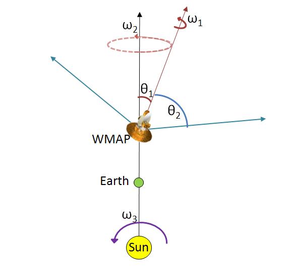
Figure 1: WMAP satellite spin and scan strategy is described in the above figure. The blue arrows: the line of sight of two horns. Red arrow: space craft symmetric axis. Black arrow: sun-WMAP line. $\theta_{1}=22.5^{\circ}$, $\theta_{2}=70.5^{\circ}$, Spin rate: $\omega_{1}=2.915398\,$rad/min  Precession rate: $\omega_{2}=0.104719755\,$rad/min, Angular rate around sun: $\omega_{3}=0.000011954\,$rad/min

A schematic diagram describing the scan strategy of the WMAP satellite is shown in Fig.1. The blue arrows show the lines of sight of the two telescopes. These two line of sight directions are denoted by $\hat{R}_{1}$ and $\hat{R}_{2}$. Some straight forward coordinate transformations can show that the direction vector $\hat{R}_{1}$ and $\hat{R}_{2}$ as a function of time in the ecliptic coordinate system can be obtained as

$$\hat{R}_{1} = \left[\begin{array}[]{ccc}\cos\omega_{1}t&\sin\omega_{1}t&0\\ -\sin\omega_{1}t&\cos\omega_{1}t&0\\ 0&0&1\end{array}\right]\left[\begin{array}[]{ccc}1&0&0\\ 0&\cos\omega_{2}t&\sin\omega_{2}t\\ 0&-\sin\omega_{2}t&\cos\omega_{2}t\end{array}\right]\left[\begin{array}[]{ccc}\cos\theta_{1}&0&\sin\theta_{1}\\ 0&1&0\\ -\sin\theta_{1}&0&\cos\theta_{1}\end{array}\right]$$ (21)

$$\times\left[\begin{array}[]{c}\cos\theta_{2}\\ \sin\theta_{2}\cos\omega_{3}t\\ \sin\theta_{2}\sin\omega_{3}t\end{array}\right]\;.$$

and

$$\hat{R}_{2} = \left[\begin{array}[]{ccc}\cos\omega_{1}t&\sin\omega_{1}t&0\\ -\sin\omega_{1}t&\cos\omega_{1}t&0\\ 0&0&1\end{array}\right]\left[\begin{array}[]{ccc}1&0&0\\ 0&\cos\omega_{2}t&\sin\omega_{2}t\\ 0&-\sin\omega_{2}t&\cos\omega_{2}t\end{array}\right]\left[\begin{array}[]{ccc}\cos\theta_{1}&0&\sin\theta_{1}\\ 0&1&0\\ -\sin\theta_{1}&0&\cos\theta_{1}\end{array}\right]$$ (35)

$$\times\left[\begin{array}[]{c}\cos\theta_{2}\\ -\sin\theta_{2}\cos\omega_{3}t\\ -\sin\theta_{2}\sin\omega_{3}t\end{array}\right]\;.$$

Here $\theta_{1},\theta_{2},\omega_{1},\omega_{2}$ and $\omega_{3}$ are as shown in the schematic diagram given in Fig.1. The values of these angles and the rotation rates are

$\theta_{1}=22.5^{\circ}$

$\theta_{2}=70.5^{\circ}$

$\omega_{1}=2.915398\,$ rad/min

$\omega_{2}=0.104719755\,$ rad/min

$\omega_{3}=0.000011954\,$ rad/min

The line of sight directions $\hat{R}_{1}$ and $\hat{R}_{2}$ are shown in green colour in Fig.2. The perpendicular direction to these two vectors is given by

$$\hat{Z}=-\hat{R}_{1}\times\hat{R}_{2}\;.$$ (36)

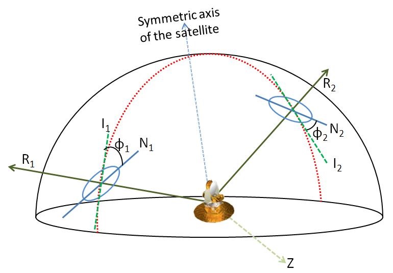
Figure 2: Beam of the WMAP satellite. $R_{1}$ and $R_{2}$ are the line of sight of the two beams. $I_{1}Z$ and $I_{2}Z$ planes are perpendicular to $R_{1}$ and $R_{2}$ respectively. The beams are located in the $I_{1}Z$ and $I_{2}Z$ plane; and $N_{1}$ and $N_{2}$ are the direction of the scan axis of the beams. $\phi_{1}$ and $\phi_{2}$ are showing the orientation of $N_{1}$ and $N_{2}$ with respect to $I_{1}$ and $I_{2}$.

For measuring the beam orientation it is important to have two independent perpendicular direction to $\hat{R}_{1}$ and $\hat{R}_{2}$. Lets us consider that the direction which is perpendicular to both $\hat{R}_{1}$ and $\hat{Z}$ and lies on the surface of the sphere centering WMAP is given by $I_{1}$ . The similar direction corresponding to $\hat{R}_{2}$ directions is given by $\hat{I}_{2}$. These two directions $\hat{I}_{1}$ and $\hat{I}_{2}$ can be calculated as

$$\hat{I}_{1}=\hat{R}_{1}\times\hat{Z}\;.$$ (37)

$$\hat{I}_{2}=\hat{R}_{2}\times\hat{Z}\;.$$ (38)

Considering that semi-major axes of the non-circular beams are aligned at an angle $\varphi_{1}$ and $\varphi_{2}$ with the directions $\hat{I}_{1}$and $\hat{I}_{2}$ respectively, the directions of the semi-major axis ($\hat{N}_{1}$ and $\hat{N}_{2}$) of the two beams are given by

$$\hat{N}_{1}=\cos\varphi_{1}\hat{I}_{1}+\sin\varphi_{1}\hat{Z}\;.$$ (39)

$$\hat{N}_{2}=\cos\varphi_{2}\hat{I}_{2}+\sin\varphi_{2}\hat{Z}\;.$$ (40)

The directions $\hat{N}_{1}$ and $\hat{N}_{2}$ are shown in blue colour in the Fig.2. The scan path of one of the beam for one complete precession is shown in Fig.3.

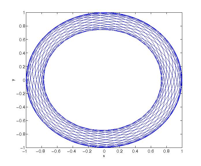
Figure 3: Scan path of one beam on the sky

In the previous section, the coordinate system is chosen such a way that the dipole in that coordinate system comes out to be $T_{0}Y_{1}^{0}(\gamma)$, i.e. the dipole is oriented along the $z-axis$ of the coordinate system. However the scan strategy discussed here is in the ecliptic coordinate system. Therefore, to apply the beam convolution technique, we need to transform all these formulae to the dipole coordinate system (the coordinate system where the $z-axis$ is oriented along the dipole). This can be done by multiplying the vectors with Euler rotation matrix. The rotation matrix for this transformation can be written as

$$\tilde{W}=\left[\begin{array}[]{ccc}-0.9703&\;\;0.1394&-0.1974\\ -0.1036&-0.9779&-0.1815\\ -0.2184&-0.1557&\;\;0.9634\\ \end{array}\right]\;.$$ (41)

Now as $\hat{R}_{1i}$, $\hat{R}_{2i}$, $\hat{N}_{1i}$ and $\hat{N}_{2i}$ are known in the dipole coordinate we can calculate $\theta_{1i}$, $\theta_{2i}$, $\rho_{1i}$ and $\rho_{2i}$ respectively and hence we can calculate the $\cos\theta_{1i}$, $\cos\theta_{2i}$, $\sin\theta_{1i}$$\cos\rho_{1i}$, $\sin\theta_{2i}$$\cos\rho_{2i}$, $\sin\theta_{1i}$$\sin\rho_{1i}$ and $\sin\theta_{2i}$$\sin\rho_{2i}$ respectively. In these expressions the subscript $1$ and $2$ represents the two beam and the subscript $i$ stands for the $i^{th}$ time step. Eq.(7) shows that the three independent TOD for each beam can be calculated independently and then after multiplying three independent TODs with the beam harmonic coefficients $b_{10}(z)$, $b_{r}(z)$ and $b_{i}(z)$, and then using some map-making technique we can thus calculate three independent maps. Those maps can be summed up to get a final map, which can be analyzed to know how much power is leaked from the dipole to the quadrupole.

4 Beam functions

The WMAP satellite scans the sky temperature in 5 different frequency bands, named as $K$, $Ka$, $Q$, $V$ and $W$ . Amongst them $Q$ and $V$ band have two detectors each and $W$ band has four detectors. Each of these detectors has one pair of beams. None of these beams are reflectional symmetric, which gives the non-zero values of $b_{r}(z)$ and $b_{i}(z)$. In Fig.5 we show the zoomed up view of the W1A side beam map. It can be seen that apart from the central peak there are many other small structures in the beam. There is a small shoulder and an annular noisy part. In the annular part there are some sections where the sensitivity of the beam is even negative. Therefore, in a large scale even if the beams are looking symmetric there is in principle no symmetry at all. This leads to nonzero value of the parameters $b_{r}(z)$ and $b_{i}(z)$. Here also it should be noted that the nonzero values of these coefficients mainly arise from the annular part around the central peak. Therefore, the size of the central peak of the beam does not matter much in determining the values of these coefficients. For doing the calculations we chose the maximum value of the beam as the center of the coordinate system. If the center changes then the values will differ significantly. In Fig.4 we have plotted one pair of beam of each of the detectors.

If $b(z,\gamma)$ be the beam function then the above harmonic coefficients of the beam can be calculated by integrating the beam with the corresponding conjugate spherical harmonics. This gives

$$b_{10}(z)=\int b(z,\gamma)Y_{10}^{*}(\gamma)d\gamma\;.$$ (42)

$$b_{r}(z)=\int b(z,\gamma)\frac{1}{2}\left(Y_{1,1}(\gamma)-Y_{1,-1}(\gamma)\right)d\gamma\;.$$ (43)

$$b_{i}(z)=\int b(z,\gamma)\frac{i}{2}\left(Y_{1,1}(\gamma)+Y_{1,-1}(\gamma)\right)d\gamma\;.$$ (44)

The values of these beam spherical harmonic coefficients for different beams have provided. Table1 have been estimated from beam maps released by WMAP.

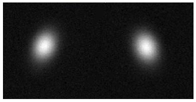
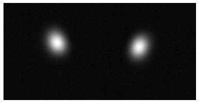
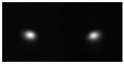
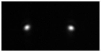
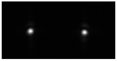
Figure 4: The figure shows beam shapes of $K_{1}$, $Ka_{1}$, $Q_{1}$, $V_{2}$ and $W_{4}$ respectively.

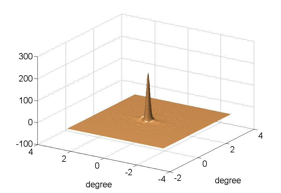
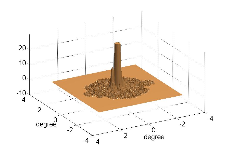
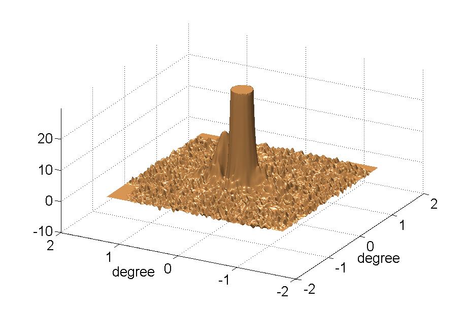
Figure 5: The left figure shows the enlarged plot of the A side beam of W1 band. The figure at the center shows a zoomed up view of the central part of this beam. The figure at the right is a more enlarged view. The figure shows that apart from the central peak the beam consists of many other small structures. These small structures spread over $\pm 4^{o}$. In some of the noisy parts the sensitivity of the beam is even negative.

5 Simulation procedure for WMAP

In this section we provide the stepwise description of the full simulation procedure. The WMAP satellite scans the full sky once in 6 months. Here a full year scan has been considered just to guarantee that no symmetry gets violated. Healpix-2.15 [11] has been used for carrying out all the simulations. The steps follows in the simulation are as follows

1. Consider a time step $t=t_{i}$

2. Calculate $\hat{R}_{1}(t_{i})$, $\hat{R}_{2}(t_{i})$, $\hat{N}_{1}(t_{i})$ and $\hat{N}_{2}(t_{i})$ using Eq.(21) - eq(40) and convert the quantities in a coordinate system in which the dipole is aligned along the $z$ axis. Here the suffix $1$ and $2$ denotes the two beams.

3. Evolute the quantities $\cos\theta_{1i}$, $\cos\theta_{2i}$, $\sin\theta_{1i}$$\cos\rho_{1i}$, $\sin\theta_{2i}$$\cos\rho_{2i}$, $\sin\theta_{1i}$$\sin\rho_{1i}$ and $\sin\theta_{2i}$$\sin\rho_{2i}$ respectively.

4. Find out the pixels $p_{1i}$ and $p_{2i}$ in the directions $\hat{R}_{1}(t_{i})$ and $\hat{R}_{2}(t_{i})$ respectively.

5. Generate the three time order data stream. The data vector will consists of the quantity $\tilde{d}_{i}^{1}=b_{0}^{A}\cos\theta_{1i}-b_{0}^{B}\cos\theta_{1i}$, $\tilde{d}_{i}^{2}=b_{r}^{A}\sin\theta_{1i}\cos\rho_{1i}-b_{r}^{B}\sin\theta_{2i}\cos\rho_{2i}$ and $\tilde{d}_{i}^{3}=b_{i}^{A}\sin\theta_{1i}\sin\rho_{1i}-b_{i}^{B}\sin\theta_{2i}\sin\rho_{2i}$.

6. Generate the $i^{th}$ row of the pointing matrix $A$ by putting $+1$ in $p_{1i}^{th}$ column and $-1$ in $p_{2i}^{th}$ column and putting $0$ in all the other columns.

7. Repeat steps 1-6 for the next time step $t=t_{i+1}$. Scan the entire sky for full year using this method.

Using the steps discussed above the pointing matrix $A$ and the three data vector $\tilde{d}^{1}$, $\tilde{d}^{2}$ and $\tilde{d}^{3}$ can be calculated. Three maps can be generated using the three time order data stream. The map-making algorithm has been discussed in the following section. Then those maps can be summed up to get the scanned sky map.

6 WMAP Map making

For WMAP TOD the differential map-making technique is required as WMAP measures the temperature difference of the sky between two points separated by $~{}141\text{\textdegree}$. Different map-making techniques are discussed in [4]. If the actual temperature of the pixelated sky at different direction is given by $\tilde{T}$ vector then

$$\tilde{d}=A\tilde{T}+\tilde{T}_{n}\;.$$ (45)

Here $\tilde{T}_{n}$ is the noise matrix. No noise is considered for this exercise as the noise will not affect such low multipole much and hence $\tilde{T}_{n}=0$.

The estimated skymap, $\hat{\tilde{T}}$ can be calculated from the TOD by taking the pseudo inverse the matrix $A$, i.e.

$$\hat{\tilde{T}}=[A^{T}A]^{-1}A^{T}\tilde{d}\;.$$ (46)

The pointing matrix $A$ is a matrix of order $N_{t}\times N_{p}$, where $N_{t}$ is the number of elements in the TOD and $N_{p}$ is the number of pixels in the map. Its not time efficient to invert the matrix $[A^{T}A]^{-1}$ using brute force method. Therefore, some iterative method, such as Jacobi iteration or conjugate gradient method has to be used to solve the equation $\tilde{d}=A\hat{\tilde{T}}.$ In this exercise we use Jacobi iterator method for solving the equation set. The mathematical details of the method are discussed in [4]. The equation used in the iteration method is

$$\hat{\tilde{T}}_{i+1}=\hat{\tilde{T}}_{i}+[\rm diag(A^{T}A)]^{-1}A^{T}(\tilde{d}-A\hat{\tilde{T}}_{i})\;.$$ (47)

Here the suffix $i$ stands for the $i^{th}$ iteration step. For initializing the iteration i.e. $\hat{\tilde{T}}_{0}$ we have taken a dipole map similar to the dipole used in the exercise. It makes the convergence faster. Here ‘tilde’ is used to denote a vector.

7 Simulation and Results from WMAP scan pattern

The simulations are done with a dipole map, similar to the CMB dipole. In the galactic coordinate the CMB dipole is oriented along $(l,b)=(264.31^{o},48.05^{o})$ and has an amplitude of $3.358\,$mK. The shape of the original dipole in the galactic and the ecliptic coordinate system are shown in Fig.6. For the conversion from Galactic to Ecliptic coordinate we have chosen the epoch $2000.0$.

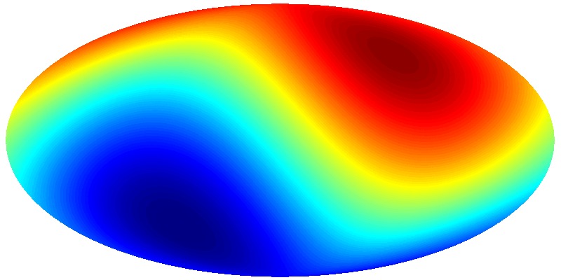
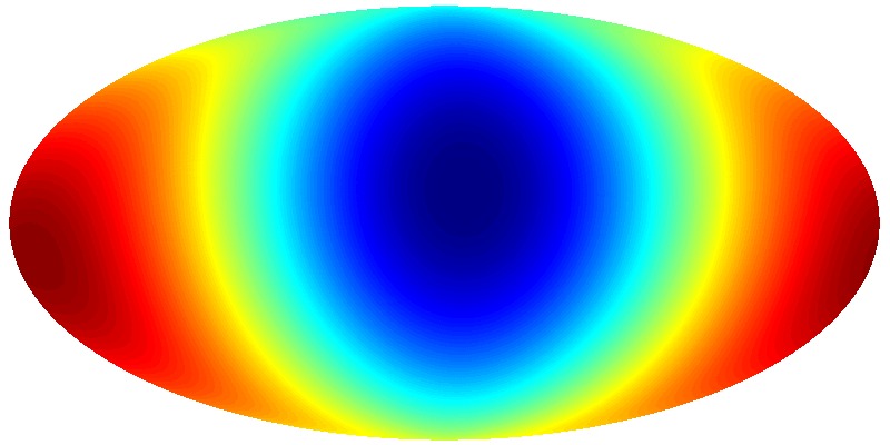
Figure 6: Shape of the original dipole in the galactic coordinate system. It is oriented along $(l,b)=(264.31^{o},48.05^{o})$ and has an amplitude of $3.358\,$mK. The figure in the left hand side is the dipole in the galactic coordinate system and in the right is in the ecliptic coordinate system

All the simulations are carried out with Healpix map having $N_{side}=256$. The values of the beam spherical harmonic coefficients i.e. $b_{r}$, $b_{i}$ along with the amount of power leakage are listed in the table 1.

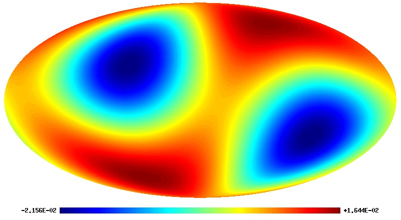
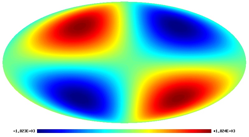
Figure 7: The left figure shows the observed quadrupole from the WMAP 9 year ILC map. The figure on the right shows the shape of the quadrupole generated while scanning the sky using W3 band. Here we have shown the W3 band because there the power leakage is maximum. It is seen that the shapes are almost similar and opposite in phase for this case. So in case of W3 band the dipole leakage will reduce the power of the quadrupole. Both the maps are in ecliptic coordinate system.

Our analysis shows that the temperature leaked from dipole into quadrupole varies for different beam maps. Also at this point we should reiterate that the coefficients involved are calculated considering the maximum sensitivity point of the beam to be the center.

But if the center is changed a bit the change it will change these coefficients and hence amount of the power leakage will also differ. In figure 7 we have shown the power leakage from W3 beam as there the power leakage is maximum. Also we have plotted the shape of the quadrupole component from the WMAP ILC map. It is seen that the shape of the quadrupole arising from the dipole power leakage is oriented similar to the measured WMAP quadrupole. Also in this particular case we see that the power leakage is in the opposite phase to the WMAP observed quadrupole. Therefore, it will decrease the power of the actual quadrupole to some extent. Though for different beams the phase of the power leakage from dipole is also different. For some of the beams the phase is opposite to the present case, but in all the cases the observed quadrupole will of course get modified by the power leakage observed here. According to the tabulated values, although the full anomaly of the dipole power leakage is small compared to the WMAP observed quadrupole, but it is sufficient enough to warrant a deeper reanalysis of the WMAP data.

Table 1: The dipole coefficients, $b_{i}$ and $b_{r}$ (imaginary and real part of $b_{1,1}$) of the beam spherical harmonics for different WMAP beams estimated from the publicly available beam maps [10]. The quadrupole temperatures (in $\mu$K) are calculated from the simulation considering the dipole temperature as 3.358 mK.

	$b^{A}_{i}$	$b^{A}_{r}$	$b^{B}_{i}$	$b^{B}_{r}$	$T_{d}$/$T_{q}$	$T_{q}$
$K_{1}$	$2.5607\times 10^{-4}$	$\-1.4374\times 10^{-4}$	$2.6614\times 10^{-4}$	$\-2.3685\times 10^{-5}$	$1332.0$	$2.52$
$Ka_{1}$	$\-1.3586\times 10^{-4}$	$\-1.7782\times 10^{-4}$	$1.9181\times 10^{-4}$	$1.3210\times 10^{-4}$	$4877.4$	$0.69$
$Q_{1}$	$2.7347\times 10^{-4}$	$\-2.4471\times 10^{-4}$	$2.2481\times 10^{-4}$	$2.2310\times 10^{-4}$	$9971.9$	$0.34$
$Q_{2}$	$1.3137\times 10^{-4}$	$2.5785\times 10^{-4}$	$1.0285\times 10^{-4}$	$\-3.2668\times 10^{-4}$	$3128.9$	$1.07$
$V_{1}$	$9.7445\times 10^{-5}$	$\-5.7361\times 10^{-5}$	$1.2977\times 10^{-4}$	$4.9800\times 10^{-5}$	$28471.0$	$0.12$
$V_{2}$	$8.3559\times 10^{-5}$	$2.0304\times 10^{-4}$	$5.3100\times 10^{-5}$	$\-1.9383\times 10^{-4}$	$\-23371.9$	$\-0.14$
$W_{1}$	$\-3.2778\times 10^{-9}$	$\-8.8946\times 10^{-5}$	$7.1132\times 10^{-5}$	$8.2677\times 10^{-6}$	$2667.9$	$1.30$
$W_{2}$	$1.1229\times 10^{-4}$	$4.1406\times 10^{-5}$	$2.4500\times 10^{-4}$	$\-7.2525\times 10^{-5}$	$6906.8$	$0.49$
$W_{3}$	$6.0105\times 10^{-6}$	$3.8637\times 10^{-5}$	$1.7441\times 10^{-4}$	$8.0611\times 10^{-5}$	$\-1810.5$	$\-1.85$
$W_{4}$	$\-2.9485\times 10^{-6}$	$4.6408\times 10^{-5}$	$1.7337\times 10^{-4}$	$9.2698\times 10^{-6}$	$\-3868.9$	$\-0.87$

8 Simulations for Planck scan strategy and results

The Planck scan strategy is different from that of the WMAP scan strategy. Planck has only one beam and thus instead of the differential measurement it measures the real temperature of the sky. The Planck satellite beam is approximately $85^{o}$ off symmetric axis and the precession angle for the satellite is around $7.5^{o}$. The precession rate is taken as one revolution per six month and the spin rate as $180^{o}/\min$. A set of similar steps as that of WMAP can be followed for analyzing the Planck scan strategy, though the parameter set for this case is

$\theta_{1}=7.5^{\circ}$

$\theta_{2}=85^{\circ}$

$\omega_{1}=0.000011954\,$ rad/min

$\omega_{2}=2\omega_{1}$

$\omega_{3}=3.14159\,$ rad/min

So using the above parameter set the value of the $\hat{R}$ can be calculated. However as there is only one beam therefore here it is not possible to take the cross product of the two beams and calculate the perpendicular direction $\hat{Z}$. Therefore, in this case the symmetric axis of the satellite is taken as $\hat{S}$. Then the perpendicular direction $\hat{Z}$ is defined by taking the cross product of $\hat{R}$ and $\hat{S}$, i.e.

$$\hat{Z}=\hat{R}\times\hat{S}\;.$$ (48)

Once $\hat{Z}$ is calculated, $\hat{I}$ and the beam orientation $\hat{N}$ can be calculated as before.

After calculating the orientation vectors, time order data and the pointing matrices can be calculated. Unlike WMAP, Planck scan strategy is not a differential measurement and thus the pointing matrices will only have a $+1$ in each of the row and no $-1$. This makes the map making technique simple, because

$$\hat{\tilde{T}}=[A^{T}A]^{-1}A^{T}\tilde{d}\;.$$ (49)

Here $A^{T}\tilde{d}$ will be a vector of length $N_{pix}$. Its obvious that the $i^{th}$ entry in this vector is the sum of all the $d_{i}$’s when the $i^{th}$ pixel got scanned. Also $[A^{T}A]$ is a diagonal matrices here and $i^{th}$ diagonal of the matrix will contain the value that how many times the $i^{th}$ pixel got scanned. Therefore, here $\hat{\tilde{T}}$ essentially gives an average temperature of a pixel, where the average is over how many times the pixel got scanned in the entire scan process.

For Planck scan strategy we can calculate three independent maps from three independent TODs. But the values of the spherical harmonic coefficients for the Planck beam are not publicly known. Therefore, after the analysis some limit can be set on the $b_{r}$ and the $b_{i}$ parameter which can cause some significant amount of power transfer from dipole to quadrupole and higher multipoles. As $b_{10}$ and other spherical harmonic coefficients of the beam don’t cause any such power transfer therefore no such limit can be imposed on them from this simulation.

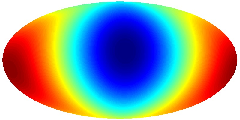
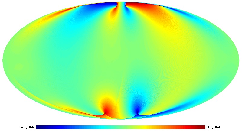
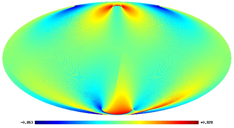
Figure 8: Three independent simulation maps from Planck scan strategy. Left one is from $\cos\theta$ component, middle one is from $\sin\theta\cos\rho$ component and the right one is from the $\sin\theta\sin\rho$ component. All these maps are in the ecliptic coordinate system.

Three independent maps which are calculated from the Planck scan strategy are shown in Fig.8. As the data of the Planck beam map is not publicly available, the amount of power leakage expected from the dipole can not be computed for the Planck scan pattern. But, from the maps which we get using the Planck scan strategy, show us that for Planck scan strategy the power leakage is not restricted to the quadrupole. The power gets transferred to all the other low multipoles also, therefore affects the low-multipole power measurement. The amount of power transfer depends on the coefficients $b_{i}$ and $b_{r}$. If the values of $b_{r}$ and $b_{i}$ are more than $10^{-4}$ then this effect may cause inaccuracy in the power measurements at the low multipoles.

9 Conclusion

An analytical formalism has been developed to use in simulations of scan strategy to estimate the leakage of power from dipole to the quadrupole and higher multipoles. It has also been shown that the power leakage only depends on the two spherical harmonic coefficients of the satellite beam ($b_{i}$ and $b_{r}$) and therefore if the beam has been designed in such a way that these two parameters of the beam are small enough then power leakage will be negligible. For WMAP, the amount of the power leakage is found to be small but not insignificant compared to the low value of quadrupole measured. The leakage of power depends on the scan pattern. For WMAP scan pattern the power leakage is mainly restricted to the quadrupole. However, for Planck scan pattern the power gets leaked to quadrupole and octapole and other higher multipoles.

References

References

- [1] A. Moss, D. Scott and K. Sigurdson 2011, JCAP,1, 1.
- [2] Feng B and Zhang X, 2003 Phys. Lett. B 570 145 [astro-ph/0305020].
- [3] R. K. Jain, P. Chingangbam, J.O. Gong, L. Sriramkumar and T. Souradeep, JCAP 0901 , 009 (2009).
- [4] J-Ch Hamilton 2003 C.R. Physique 4 871 [astro-ph/0310787].
- [5] P. Fosalba, O. Dor, and F.R. Bouchet, Phys. Rev. D 65, 063003 (2002).
- [6] S. Mitra, A.S. Sengupta, T. Souradeep PhRvD, 70 (2004), p. 103002.
- [7] T. Souradeep and B. Ratra, Astrophys. J. 560, 28 (2001).
- [8] T. Souradeep, S. Mitra, A. S. Sengupta, S. Ray, R. Saha, New Astron. Rev. 50, 2006.
- [9] G. Hinshaw et al., Astrophys. J. Suppl. 170, 288 (2007).
-
[10]
The beam maps can be found on
www.lambda.gsfc.nasa.gov/product/map/dr3/beam_profiles_get.cfm. -
[11]
Hierarchical Equal Area isoLatitude Pixelization
http://healpix.jpl.nasa.gov/.