Universal time-fluctuations in near-critical out-of-equilibrium quantum dynamics

Abstract

Out of equilibrium quantum systems, on top of quantum fluctuations, display complex temporal patterns. Such time fluctuations are generically exponentially small in the system volume and can be therefore safely ignored in most of the cases. However, if one consider small quench experiments, time fluctuations can be greatly enhanced. We show that time fluctuations may become stronger than other forms of equilibrium quantum fluctuations if the quench is performed close to a critical point. For sufficiently relevant operators the full distribution function of dynamically evolving observable expectation values, becomes a universal function uniquely characterized by the critical exponents and the boundary conditions. At regular points of the phase diagram and for non sufficiently relevant operators the distribution becomes Gaussian. Our predictions are confirmed by an explicit calculation on the quantum Ising model.

Introduction

Low temperature quantum matter at equilibrium organizes itself in different phases separated by critical regions featuring enhanced quantum fluctuations patashinskii_fluctuation_1979 ; sachdev_quantum_2011 . This is due to the existence of competing interaction terms in the system’s Hamiltonian each of which strives to order the system according different symmetry patterns. When the system is taken out-of-equilibrium e.g., by a sudden change of the Hamiltonian parameters, on top of these quantum fluctuations, temporal fluctuations are present as well. In a series of papers campos_venuti_unitary_2010 ; campos_venuti_universality_2010 ; campos_venuti_exact_2011 ; campos_venuti_gaussian_2013 we have shown that the full time-statistics of a dynamically evolving expectation value ${\cal A}(t)$ of a quantum observable $A$ provides a wealth of information about the equilibration properties of the system, finite-size precursors of quantum criticality campos_venuti_universality_2010 as well as a tool to single out quantum integrability in an operational fashion campos_venuti_gaussian_2013 .

Let us start by setting the general stage of our investigations. Consider a quantum system driven out of equilibrium by an Hamiltonian $H$ and evolving unitarily according to the Schrödinger equation ($\rho\left(t\right)=e^{-itH}|\psi_{0}\rangle\langle\psi_{0}|e^{itH}$). For definiteness we will focus on a many-body quantum system defined on a $d$-dimensional lattice of volume $V$, and $A$ being a local extensive observable. A first natural question is now: what is the typical size of temporal fluctuations $\mathcal{A}(t)=\mathrm{tr}\left[A\rho\left(t\right)\right]$ ? Reimann in (reimann_foundation_2008, ; reimann_equilibration_2012, ) has proven, assuming the non-resonant condition for the energy gaps, the following bound on the temporal variance of $\mathcal{A}$ :

$$\Delta\mathcal{A}^{2}:=\overline{\left(\mathcal{A}\left(t\right)-\overline{\mathcal{A}}\right)^{2}}\leq\mathrm{diam}\left(A\right)^{2}\mathrm{tr}\left(\overline{\rho}^{2}\right).$$ (1)

where $\mathrm{diam}(A)$ is the diameter of the spectrum of $A,$ a measures of the strength of $A$. As shown in (campos_venuti_gaussian_2013, ) (see also gambassi_large_2012 ; zangara_time_2013 ), for clustering initial states, $\mathrm{tr}\left(\overline{\rho}^{2}\right)\lesssim e^{-\alpha V}$ so that the normalized fluctuations $\Delta\mathcal{A}/\overline{\mathcal{A}}$ are bounded by $\Delta\mathcal{A}/\overline{\mathcal{A}}\lesssim e^{-\alpha V}$. This shows that in this general situation time fluctuations are practically absent and one can safely replace dynamically evolving quantities $\mathcal{A}(t)$ with their averages, i.e. $\mathcal{A}(t))\simeq\overline{\mathcal{A}}$ i.e., equilibration is achieved.

However, there are at least two situations in which time fluctuations are greatly enhanced and in some cases may become even stronger than equilibrium ones. One possibility is to consider systems of non-interacting particles. The bound (1) does not apply in this case and rather a “Gaussian equilibration” scenario sets in whereby time fluctuations are seen to scale as $\Delta\mathcal{A}/\overline{\mathcal{A}}\sim V^{-1/2}$ (campos_venuti_gaussian_2013, ) (see also cassidy_generalized_2011 ; gramsch_quenches_2012 ; he_single-particle_2013 ; zangara_time_2013 ). This seems to be a precise prediction of the folklore according to which free systems show poor equilibration.

Another possibility is offered by a small quench experiment. With this we mean to tune the initial state to be the ground state of a given Hamiltonian and then perform a small sudden change in the Hamiltonian parameters. Intuitively, if the quench is sufficiently small only relatively few quasi-particles get excited and contribute to the equilibration process. This in turn results in poor equilibration property, i.e. large time fluctuations. Roughly speaking this is a region of parameters for which $\alpha V\lesssim 1$ and so the bound (1) becomes ineffective. As shown in (campos_venuti_universality_2010, ) this situation can be used to locate precursor of criticality on small systems by looking at dynamically evolving quantities.

In this Letter we will analyze this infinitesimal quench scenario in detail and show that the full time-probability distributions of (properly rescaled) expectation values of observables feature a novel type of universality in the infinite-volume limit. For sufficiently relevant operators the full distribution function become a universal function uniquely characterized by the critical exponents and the boundary conditions. Whereas, for non sufficiently relevant operators or at regular point of the phase diagram the distribution becomes Gaussian.

Observable dynamics for small quench

Consider then the following small quench scenario. The system is prepared in the ground state of the Hamiltonian $H_{0}$ for $t<0$. At time $t=0$ one suddenly switches on a small perturbation $B$ such that the evolution Hamiltonian becomes $H=H_{0}+\delta\lambda B$, with $\delta\lambda$ a small parameter . Expanding ${\cal A}(t)$ up to first order in $\delta\lambda$ using Dyson expansion and the spectral resolution $H_{0}=\sum_{n}E_{n}|n\rangle\langle n|$, one gets

$${\cal A}(t)=\overline{A}+\delta\lambda\sum_{n>0}\left(Z_{n}e^{-it(E_{n}-E_{0})}+\mathrm{c.c.}\right)+O\left(\delta\lambda^{2}\right),$$ (2)

where the first, time-independent term is the average of $\mathcal{A}\left(t\right)$ and with $Z_{n}:=A_{0,n}B_{n,0}/\left(E_{n}-E_{0}\right)$. The leading contribution to the temporal variance is therefore at second order and assuming that the gaps $E_{n}-E_{0}$ are non-degenerate one obtains

$$\Delta\mathcal{A}_{B}^{2}=2\delta\lambda^{2}\sum_{n>0}\left|Z_{n}\right|^{2}+O\left(\delta\lambda^{3}\right).$$ (3)

We added a subscript $B$ to recall that the variance is computed with perturbation $B$. Eq. (3) shows a intriguing similarity to the zero temperature equilibrium isothermal susceptibility defined by $\langle\psi\left(\delta\lambda\right)|A|\psi\left(\delta\lambda\right)\rangle=\langle\psi\left(0\right)|A|\psi\left(0\right)\rangle+\delta\lambda\chi_{AB}+O\left(\delta\lambda^{2}\right)$ ($|\psi\left(\delta\lambda\right)\rangle$ being the ground state of $H$). Indeed we can write $\chi_{AB}=2\sum_{n>0}\mathrm{Re}Z_{n}.$ Inasmuch a super-extensive scaling of the susceptibility can be used to detect criticality the same can be said for the time fluctuations.

Using Eq. (2) we can actually obtain the full probability distribution of the variable $\mathcal{A}$. Assuming rational independence (RI) of the gaps $E_{n}-E_{0}$ and using the theorem of averages we can express the time average as a phase space average over a large dimensional torus. We then obtain, for the characteristic function of $\mathcal{A}$,

$$\overline{e^{is(\mathcal{A}-\overline{\mathcal{A}})/\delta\lambda}}=\prod_{n>0}J_{0}\left(2s\left|Z_{n}\right|\right):=J^{\mathcal{A}}\left(s\right),$$ (4)

where $J_{0}$ is the Bessel function of the first kind. So the probability distribution of $\mathcal{A}$ is completely encoded in the function $J^{\mathcal{A}}\left(s\right)$. Let us also define the Wick rotated function $I^{\mathcal{A}}\left(s\right)=J^{\mathcal{A}}\left(is\right)$ which has the advantage of being positive for real $s$. We can then define the coefficients $a_{n}$ by the series $\ln\left[I_{0}\left(s\right)\right]=\sum_{n=1}^{\infty}a_{n}s^{n}/n!$ which converges absolutely in a neighborhood of the origin. Note that $a_{p}=0$ for $p$ odd. The cumulant of the variable $(\mathcal{A}-\overline{\mathcal{A}})/\delta\lambda$ are given by $\kappa_{2p}=a_{2p}2^{2p}Q_{2p}$ with $Q_{2p}:=\sum_{n>0}\left|Z_{n}\right|^{2p}$ (odd cumulants are zero). Under the assumption of convergence the probability distribution of $\mathcal{A}$ is uniquely characterized by the coefficients $Q_{2p}$. Conversely the probability distribution uniquely defines the coefficients $Q_{2p}$ which are generalizations of the variance Eq. (3). Intuitively, at critical points the cumulants $\kappa_{2p}$ (through the coefficients $Q_{2p}$) tend to diverge with the system size, higher cumulant being more divergent.

Let us analyze the behavior of $Q_{2p}$ close to quantum criticality. In this case $\delta\lambda=\left|\lambda-\lambda_{c}\right|$ measures the distance from the critical point $\lambda_{c}$. Using standard scaling arguments one can show that $Q_{2p}\propto L^{2p\alpha}$ with $\alpha=2d+\zeta-\Delta_{A}-\Delta_{B}$ (see Supplemental Material). Here $\Delta_{A/B}$ are the scaling dimensions of the observables $A/B$ that we assumed extensive and $\zeta$ is the dynamical critical exponent. Instead, away from criticality the expectation is $Q_{2p}\propto L^{d}$. Requiring that, at finite size, $Q_{2p}$ is analytic in the system parameters and matches the above scaling, one can predict the behavior of $Q_{2p}$ close to the critical point both in the critical region $\xi\gg L$ and in the off-critical one $\xi\ll L$:

$$\kappa_{2p}\sim Q_{2p}\sim\begin{cases}L^{2\alpha p}&\xi\gg L\\ \delta\lambda^{d\nu-2\alpha p\nu}L^{d}&\xi\ll L\end{cases}\,.$$ (5)

Let us compare the strength of the temporal fluctuations encoded in Eq. (5) with other familiar forms of quantum fluctuations close to criticality. Equilibrium quantum fluctuations of an observable $A$ in a state $|\psi\rangle$ are encoded in the cumulants $\langle A^{n}\rangle_{c}$ where the subscript $c$ denotes connected averages with respect to $|\psi\rangle$. In the critical region the singular part of these cumulants scales as $L^{n(d-\Delta_{A})}$ where $\Delta_{A}$ is the scaling dimension of $A$ (campos_venuti_unitary_2010, ). When one is interested in the response to a perturbation $A$ encoded in a Hamiltonian $H=H_{0}+\lambda A$, other generalized cumulants are given by the higher order susceptibilities $\partial^{n}E/\partial\lambda^{n}$ ($E$ is the ground state of $H$, or the free energy at positive temperature). At criticality such generalized susceptibilities grow as $L^{-\zeta+n/\nu}$, in particular one as $L^{2d+\zeta-2\Delta_{A}}$ for $n=2$. Comparing with Eq. (6) we see that temporal fluctuations –which are basically absent for general quenches– become the strongest fluctuations for small quenches close to criticality. Indeed, looking at the scaling of the variances (and setting $A=B$ for simplicity) the exponents for the temporal variance, susceptibilities and quantum variance satisfy $2(2d+\zeta-2\Delta_{A})>(2d+\zeta-2\Delta_{A})>2d-2\Delta_{A}$. As noted in (campos_venuti_universality_2010, ) this opens up the possibility of observing dynamical manifestations of criticality on small systems.

Consider now the rescaled random variable $\mathcal{R}\left(t\right)=(\mathcal{A}\left(t\right)-\overline{\mathcal{A}})/\Delta\mathcal{A}$ whose cumulants are given by $\kappa_{2n}^{\mathcal{R}}=\kappa_{2n}^{\mathcal{A}}/(\kappa_{2}^{\mathcal{A}})^{n}$ for $n\geq 1$ whereas odd cumulants are zero. The probability distribution of $\mathcal{R}$ is uniquely determined by the ratios $R_{2p}=Q_{2p}/\left(Q_{2}\right)^{p}$. From Eq. (5) we see that in the quasi-critical regime, these ratios are scale independent and define some presumably universal constants. Let us now find these constants. With the help of density of states $\rho\left(E\right)=\mathrm{tr}\left(\delta\left(H-E\right)\right)$ we can write $Q_{p}=\int Q_{p}\left(E\right)\rho\left(E\right)dE$. Since $\rho\left(E\right)dE$ is scale invariant, from $Q_{p}\propto L^{p\alpha}$ we derive $Q_{p}\left(E\right)\propto E^{-p\alpha/\zeta}$. In order to proceed further we must assume the form of the low energy dispersion. The simplest possibility is a rotationally invariant spectrum at small momentum $E\simeq C\left\|\boldsymbol{k}\right\|^{\zeta}=C(\sum_{j}k_{j}^{2})^{\zeta/2}$ where $\boldsymbol{k}$ is a quasi-momentum vector. In one dimension this is essentially the only possibility but for $d>1$ one can also have anisotropic transitions where the form of the dispersion depends on the direction. Using the isotropic assumption we obtain $Q_{p}\simeq C^{\prime}\sum_{\boldsymbol{k}}\left\|\boldsymbol{k}\right\|^{-p\alpha}.$ In doing so we have essentially restricted the sum over $n$ to the one-particle contribution. This is expected to be the leading contribution whereas higher particle sectors contribute at most to the extensive, regular term. At this point, a part from an irrelevant constant $C^{\prime}$, the behavior of the cumulants is uniquely specified by the critical exponent $\alpha$ and the boundary conditions that specify $\boldsymbol{k}$. More precisely the probability distribution of the rescaled variable $\mathcal{R}\left(t\right)$ is a universal function which depends only on $\alpha$ and the boundary conditions. Let us be more explicit. Assume for concreteness that the lattice is a hyper-cube of size $L$ and the boundary conditions (BC) are such that moments are quantized according to $\boldsymbol{k}=(2\pi/L)(\boldsymbol{n}+\boldsymbol{b})$ with $n_{i}=1,\ldots,L$. The BC on the direction $i$ are fixed by $b_{i}\in\left[0,1/2\right]$ which interpolate between periodic (PBC, $b_{i}=0$) and anti-periodic (ABC, $b_{i}=1/2$) BC. Define now the generalized $d$-dimensional Hurwitz-Epstein $\zeta$-function as $\zeta_{\boldsymbol{b}}\left(\alpha\right)=\sum_{n_{1}=1}^{\infty}\cdots\sum_{n_{d}=1}^{\infty}\left\|\boldsymbol{n}+\boldsymbol{b}\right\|^{-\alpha}$. The cumulants of $\mathcal{R}$ depend on the universal ratios $R_{2p}=Q_{2p}/\left(Q_{2}\right)^{n}$ which are given by (letting $L$ go to infinity) $R_{2p}=\zeta_{\boldsymbol{b}}\left(2p\alpha\right)/\zeta_{\boldsymbol{b}}\left(2\alpha\right)^{p}$. For example, in $d=1$ and for PBC one has $R_{2p}=\zeta\left(2p\alpha\right)/\zeta\left(2\alpha\right)^{p}$ where $\zeta\left(\alpha\right)$ is the familiar Riemann zeta function. Clearly, anisotropic energy dispersion can also be treated introducing even more general zeta functions with different exponents in different directions. So far the exponent $\alpha$ has been quite arbitrary. Indeed $\alpha$ can even become negative if $A$ and $B$ are not sufficiently relevant. For example $\alpha=-\zeta$ if both $A$ and $B$ are marginal operators. Apparently the moments of $\mathcal{R}$ become not normalizable in this case. The correct procedure is to keep the sum over $\boldsymbol{k}$ finite, compute the leading finite size correction, calculate the ratios $R_{2p}$ and then take the infinite volume limit. The result is

$$\lim_{L\to\infty}R_{2p}=\begin{cases}\delta_{p,1}&2\alpha\leq d\\ \zeta_{\boldsymbol{b}}\left(2p\alpha\right)/\zeta_{\boldsymbol{b}}\left(2\alpha\right)^{p}&2\alpha>d.\end{cases}$$ (6)

For $2\alpha\leq d$ the characteristic function of $\mathcal{R}(t)$ becomes $e^{-s^{2}/2}$ in the thermodynamic limit and so $\mathcal{R}$ tends in distribution to Gaussian. Clearly the Gaussian behavior observed here for not sufficiently relevant operators, is also to be expected at regular points of the phase diagram. A discussion of the regular points as well as a comparison of the dynamical central limit type theorem here discussed and the one for quantum fluctuations at equilibrium can be found in the Supplemental Material.

Loschmidt echo

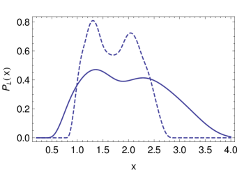
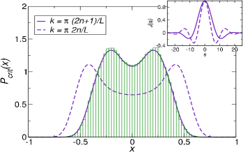
Figure 1: Upper panel: Universal probability distribution for the Loschmidt echo in one dimension for different $\nu$ and PBC momenta i.e. $k=2\pi n/L$. Solid curve $\nu=1$ ($\alpha=2$) dashed $\nu=4/3$ ($\alpha=3/2$). The curves are obtained integrating numerically Eq. (8). Lower panel: Critical probability distribution for the quantity $[\langle M(t)\rangle-\overline{M}]/(L\delta h)$ close to the Ising critical point $h=1$. The inset shows the characteristic function $J\left(s\right)=\prod_{n=0}^{\infty}J_{0}\left(s/\left(2n+1\right)\right)$. The dashed lines are obtained using quasimomenta of the form $k=2\pi n/L$. The histogram is computed performing a numerical experiment on the Ising model on a chain of $L=1006$ sites with periodic boundary conditions. The quench parameters are $h_{1}=1$, $h_{2}=1.0003$ and $\gamma_{1}=\gamma_{2}=1$. The statistics is obtained sampling 600,000 random times uniformly sampled in $\left[0,T\right]$ with $T=600,000$. The distribution is unchanged using a different $\gamma_{1}=\gamma_{2}\neq 0$ as implied by universality.

Let us now extend the formalism by considering a particular, non-extensive observable $A=|\psi_{0}\rangle\langle\psi_{0}|.$ In this case ${\cal A}(t)$ becomes the so-called the Loschmidt echo (LE) or survival probability given by $\mathcal{L}\left(t\right)=\left|\langle\psi_{0}|e^{-itH}|\psi_{0}\rangle\right|^{2}$. The Loschmidt echo is essentially the Fourier transform of the work distribution function and is currently at the center of much theoretical work. We will show that it is possible to obtain its full time statistics exactly for a general initial state. Using the spectral resolution of $H$ the LE can be written as $\mathcal{L}\left(t\right)=\left|G\left(t\right)\right|^{2}$ with $G\left(t\right)=\sum_{n}p_{n}e^{-itE_{n}}:=X\left(t\right)+iY\left(t\right)$ where $p_{n}=\left|\langle n|\psi_{0}\rangle\right|^{2}$ and $X(t),\,Y(t)$ are its real and imaginary part. Let us start by noticing that

$$\mathrm{Prob}\left(\mathcal{L}<r\right)=\int_{x^{2}+y^{2}<r}P_{X,Y}\left(x,y\right)dxdy$$ (7)

where $P_{X,Y}\left(x,y\right)$ is the joint probability density of $X$ and $Y$, i.e. $P_{X,Y}\left(x,y\right)=\overline{\delta\left(X-x\right)\delta\left(Y-y\right)}$. The related, joint characteristic function $\chi\left(\xi,\eta\right)=\overline{e^{i\xi X}e^{i\eta Y}}$ can again be computed as a phase-space average assuming rational independence of the energies $E_{n}$. Expressing Eq. (7) in terms of $\chi\left(\xi,\eta\right)$, integrating over $x$ and $y$ and differentiating with respect to $r$ we obtain the following expression for the probability density of the Loschmidt echo (more details in the Supplemental Material)

$$P_{\mathcal{L}}\left(x\right) = \int_{0}^{\infty}K\left(x,\rho\right)J^{\mathcal{L}}\left(\rho\right)d\rho$$ (8)

$$K\left(x,\rho\right) = \frac{J_{1}\left(\sqrt{x}\rho\right)}{2\sqrt{x}}+\frac{\rho}{4}\left[J_{0}\left(\sqrt{x}\rho\right)-J_{2}\left(\sqrt{x}\rho\right)\right]$$ (9)

and $J^{\mathcal{L}}\left(\rho\right):=\prod_{n}J_{0}\left(p_{n}\rho\right).$ The probability distribution of the LE is completely encoded in the function $J^{\mathcal{L}}$. Proceeding as previously we realize that $J^{\mathcal{L}}\left(\rho\right)=\exp\left[\sum_{n}a_{n}\mathrm{tr}\left(\overline{\rho}^{n}\right)\left(-i\rho\right)^{n}/n!\right]$ where $\overline{\rho}$ is the infinite time average of $\rho\left(t\right)$. Again, under assumption of convergence, the probability distribution of $\mathcal{L}$ is uniquely specified by the numbers $\mathrm{tr}\left(\overline{\rho}^{n}\right)$ and vice-versa. Since $\overline{\rho}$ is a positive operator this uniquely specifies the spectrum of $\overline{\rho}$. Note that the average LE is given by the first term in the expansion of $J^{\mathcal{L}}\left(\rho\right)$ and is $\overline{\mathcal{L}}=\mathrm{tr}\left(\overline{\rho}^{2}\right)$. Let us first investigate the case of small quench close to a critical point. It has been shown already that, as a function of energy the weights $p\left(E_{n}\right):=p_{n}$ behave as $p\left(E\right)\sim\delta\lambda^{2}E^{-2/(\zeta\nu)}$ in the quasi-critical regime (campos_venuti_universality_2010, ; de_grandi_quench_2010, ). Using again the isotropic assumption $E\sim\left\|\boldsymbol{k}\right\|^{\zeta}$ we find $p_{\boldsymbol{k}}\sim\delta\lambda^{2}\left\|\boldsymbol{k}\right\|^{-2/\nu}$. Let us now study the rescaled LE $\mathcal{L}\left(t\right)/\overline{\mathcal{L}}$. Its distribution is determined by $J^{\mathcal{L}}(\rho/\sqrt{\overline{\mathcal{L}}})=\exp\left[\sum_{n=1}a_{2n}T_{2n}(-\rho^{2})^{n}/(2n)!\right]$ with $T_{2n}:=\mathrm{tr}\left(\overline{\rho}^{2n}\right)/\mathrm{tr}\left(\overline{\rho}^{2}\right)^{n}$. Once again, at criticality the probability distribution is uniquely determined by the scaling exponent $\nu$ and the quantization of the quasi-momenta $\boldsymbol{k}$. Moreover, taking the thermodynamic limit ($L\to\infty$) in the quasi-critical region, the rescaled cumulants $T_{2n}$ become exactly $T_{2n}=R_{2n}$ of Eq. (6) with $\alpha=2/\nu$. In particular we see that for $4\nu\leq d$ $\lim_{L\to\infty}J^{\mathcal{L}}(\rho/\sqrt{\overline{\mathcal{L}}})=\exp\left[-\rho^{2}/4\right]$. Using this expression and Eq. (8) one gets the probability distribution of the rescaled LE: $\lim_{L\to\infty}P_{\mathcal{L}/\overline{\mathcal{L}}}\left(x\right)=\vartheta\left(x\right)e^{-x}$ i.e. a Poissonian distribution. This in turns implies, for the un-rescaled variable, $P_{\mathcal{L}}\left(x\right)\simeq\vartheta\left(x\right)e^{-x/\overline{\mathcal{L}}}/\overline{\mathcal{L}}$ a result which has been observed in (campos_venuti_unitary_2010, ) (see also the recent (ikeda_emergent_2013, )). Clearly the Gaussian behavior of $J^{\mathcal{L}}$ predicted for not sufficiently relevant operators $\nu\leq d/4$ is expected to be seen also in the off-critical region. In fact, the same considerations regarding the $\mathcal{R}$ variable apply in this case. A small quench in the vicinity but not at the critical point has the effect of opening up a mass gap. This in tun cures the infra-red divergences (UV divergences are cured by the lattice) and one obtains that $\lim_{L\to\infty}T_{2n}=\delta_{n,1}$. One also expects that this behavior extends a fortiori for more general quenches. Indeed we conjecture that $\lim_{L\to\infty}T_{2n}=\delta_{n,1}$ for any sufficiently clustering initial state $|\psi_{0}\rangle$. A plot of the universal, critical distribution of the LE is shown in Fig. 1.

Computing critical distribution functions is a very hard task at equilibrium as one needs the exact analytic form of the characteristic function. For this reasons results are essentially limited to models that can be mapped to a system of non-interacting particles such as the 2D classical Ising model and its 1D quantum counterpart (see e.g. (lamacraft_order_2008, )). The situation for the temporal fluctuation is analogous and in order to exemplify the formalism we consider now the 1D quantum XY model with PBC. We perform a small quench in the transverse field close to the Ising critical point at $h=1$. The expectation value of the total magnetization takes the form $\mathcal{M}\left(t\right)=\sum_{j}\langle\sigma_{j}^{z}(t)\rangle=\overline{\mathcal{M}}+\sum_{k}\sin(\vartheta_{k}^{(2)})\sin(\delta\vartheta_{k})\cos(t\Lambda_{k})$. The function $W_{k}:=\sin(\vartheta_{k}^{(2)})\sin(\delta\vartheta_{k})$ plays the role of $Z_{n}$ in Eq. (3). The characteristic function can be computed assuming rational independence of the one particle energies and one obtains

$$\overline{e^{i\lambda(\mathcal{M}-\overline{\mathcal{M}})/\Delta\mathcal{M}}}=\exp\sum_{k}\ln\left[J_{0}\left(\lambda W_{k}/\Delta\mathcal{M}\right)\right].$$ (10)

The scaling dimensions are in this case $d=\zeta=\Delta_{A}=\Delta_{B}=1$ implying that $\sum_{n>0}\left|Z_{n}\right|^{2}\sim L^{2}$. This can be in fact proven analytically as, for small quench, $W_{k}$ is singular at $k=\pi$, where it behaves as $W_{k}\sim 1/\left|\gamma\left(k-\pi\right)\right|$. Expanding the argument of the exponential in series one realizes that only the divergent part of $W_{k}$ is needed when computing the limit $L\to\infty$. Given the fact that, for large $L$, $\Delta\mathcal{M}^{2}=2^{-1}\left(L/2\pi\right)^{2}\sum_{n=0}^{\infty}\left(n+1/2\right)^{-2}$, we then obtain $\lim_{L\to\infty}\sum_{k}\ln\left[J_{0}\left(\lambda W_{k}/\Delta\mathcal{M}\right)\right]=\sum_{n=0}^{\infty}\ln J_{0}(\lambda\alpha_{n})$, where $\alpha_{n}^{-1}:=\sqrt{\zeta_{1/2}\left(2\right)/2}\,(n+1/2)$. In figure 1 we plot the exact, critical, probability distribution of the transverse magnetization obtained Fourier transforming numerically Eq. (10). We also show very good agreement with a numerical, small quench experiment performed on a XY chain. The critical distribution is observed as long as $\xi\simeq\delta h^{-1}\gg L$ and $L\gtrsim 20$. For shorter sizes, $\mathcal{M}$ is a sum of few random variables and can be well approximated by retaining the two dominant variables (campos_venuti_universality_2010, ). In the off-critical region $\xi\ll L$ one obtains a Gaussian distribution (campos_venuti_gaussian_2013, ).

Applications

We would like now to point out the possible use of the time-fluctuations formalism to distinguish critical or gapped regions in non-homogeneous systems. A concrete realization of these systems is offered by optical lattices of cold atoms in harmonic traps. Traditionally batrouni_mott_2002 ; rigol_local_2003 ; wessel_quantum_2004 ; rigol_numerical_2004 Mott-insulating regions are distinguished from superfluid ones by looking either at the quantum fluctuations of the particle densities $\langle n_{i}^{2}\rangle-\langle n_{i}\rangle^{2}$ or at the local compressibility (or suitably averaged version thereof) $\partial\langle n_{i}\rangle/\partial\mu_{i}$, i.e. a susceptibility. Small (resp. large) fluctuations correspond to Mott-insulating, “gapped” (resp. superfluid, “critical”) regions. Indeed, as expected by the larger scaling and confirmed in (rigol_local_2003, ) the local compressibility is so far the best indicator of insulating/superfluid region. The study of temporal fluctuations for small quenches in trapped cold atom systems, may offer an experimentally accessible yet powerful way to investigate such non-homogeneous systems. The feasibility of such an approach is currently under investigation (yeshwanth__????, ).

Conclusions

In this Letter we have shown that the temporal fluctuations of quantum observables for a small Hamiltonian quench near a critical poins feature a novel type of universality that mirrors the one of quantum fluctuations at equilibrium. The initial quantum state is choesen to be the ground state of a Hamiltonian $H_{0}$ which is then slightly perturbed to $H=H_{0}+\delta\lambda B$. Given the observable $A$ the temporal probability distribution $P_{\mathrm{dyn}}(a):=\overline{\delta\left(\langle A(t)\rangle-a\right)}$ (overline denotes the infinite time average) becomes Gaussian for regular points of the phase diagram whereas it acquires a universal form at critical points. Assuming hyperscaling, the critical distribution function $P_{\mathrm{dyn}}$ is uniquely characterized by the critical exponents and the boundary conditions it is hence even more universal than the the equilibrium case. Moreover universal dynamical distributions are observed even for less relevant operators. A byproduct of this analysis is that, in the critical regime, temporal fluctuations are stronger than other forms of equilibrium quantum fluctuations. This opens up the possibility of assessing the critical character of non-homogeneous systems by performing quench experiments.

The authors wish to thank H. Saleur for precious discussions. This research was partially supported by the ARO MURI under grant W911NF-11-1-0268. PZ also acknowledges partial support by NSF grants No. PHY-969969.

Supplemental Material

.1 Small quench regime and universality

The small quench regime can be encoded by the relation  $\mathrm{tr}\left(\overline{\rho}^{2}\right)\simeq 1.$ If this condition is met the bound (1) becomes ineffective. For small quench $\mathrm{tr}\left(\overline{\rho}^{2}\right)$ can be related to the fidelity between initial and final ground state and its fidelity susceptibility $\chi_{F}$ [22]. Considering the scaling of the fidelity susceptibility $\chi_{F}$ in this regime (see [23]) one obtains $\max\delta\lambda^{2}\left\{L^{d},L^{2/\nu}\right\}\ll 1$ or $\delta\lambda\ll\min\left\{L^{-d/2},L^{-1/\nu}\right\}$ where $\delta\lambda=\lambda_{2}-\lambda_{1}$ is the quench amplitude. As is often the case, the symbol “$\ll$” indicates a conservative estimates and $\delta\lambda\sim\min\left\{L^{-d/2},L^{-1/\nu}\right\}$ indicates the region where a crossover takes place. Once the small quench condition is satisfied, universal behavior in the full time statistics of observables expectation values is expected in the quasi-critical region when $\xi^{(2)}\gg L$ where $\xi^{(2)}\simeq\left|\lambda_{2}-\lambda_{c}\right|^{-\nu}$ is the correlation length of the evolution Hamiltonian. Roughly speaking the condition to observe universal distribution can be written compactly as $\xi^{(j)}\gg L$ with $j=1,2$ . Moreover $L$ should be large enough such that i) the universality in the function $Q_{2p}(E)$ sets in and ii) the finite-size corrections to the zeta function results are small. Both of these conditions depend on the critical exponent $2\alpha$. For larger values of $2\alpha-d$, a critical, universal distribution can be observed for smaller sizes. In the opposite, off-critical region $\xi^{(2)}\ll L$, temporal distributions are expected to be of Gaussian shape [4, 5].

We have verified universality in temporal distributions on the hand of the XY model in transverse field given by the Hamiltonian

$$H=\sum_{j=1}^{L}\left[\frac{1+\gamma}{2}\sigma_{j}^{x}\sigma_{j+1}^{x}+\frac{1-\gamma}{2}\sigma_{j}^{y}\sigma_{j+1}^{y}+h\sigma_{j}^{z}\right],$$ (11)

defined on a chain of $L$ sites with periodic boundary conditions for the spins, i.e. $\sigma_{L+1}^{\alpha}=\sigma_{1}^{\alpha}$, $\alpha=x,y$. The system is initialized in the ground state of Hamiltonian (11) with parameters $h=h_{1}$ and $\gamma=\gamma_{1}$ which are then suddenly changed to $h_{2}$ and $\gamma_{2}$. The transverse magnetization at time $t$ has the form

$$\mathcal{M}(t) =\sum_{j}\langle\sigma_{j}^{z}(t)\rangle$$ (12)

$$=\sum_{k}\left[\cos(\vartheta_{k}^{(2)})\cos(\delta\vartheta_{k})+\right.$$ (13)

$$\left.\sin(\vartheta_{k}^{(2)})\sin(\delta\vartheta_{k})\cos(t\Lambda_{k})\right]$$ (14)

where $k$ are ABC momenta for the fermions: $k=2\pi/L\left(n+1/2\right)$, $n=0,1,\ldots,L-1$ and the Bogoliubov angles are given by $\tan\vartheta_{k}^{(i)}=-\gamma^{(i)}\sin(k)/(h^{(i)}+\cos(k))$ and $\delta\vartheta_{k}=\vartheta_{k}^{(2)}-\vartheta_{k}^{(1)}$.

.2 Scaling behavior

Let us write $Q_{p}=Q_{1}^{p}{\mathrm{tr}}\,\Omega^{p},$ where we have defined $\Omega:=Q_{1}^{-1}{\mathrm{diag}}\,\left(|Z_{n}|\right)_{n>0}.$ Since $\Omega$ is dimensionless the scaling behavior of $Q_{p}$ is clearly dictated by the scaling dimension of $Q_{1}^{p}$ this latter in turn is just $p$ times the one of $Q_{1}.$ Now $Q_{1}\geq|\tilde{Q}_{1}|$ where $\tilde{Q}_{1}:=\sum_{n>0}Z_{n}=\sum_{n>0}\langle 0|A|n\rangle\langle n|B|0\rangle/(E_{n}-E_{0}),$ therefore the scaling dimension $\Delta_{Q_{1}}$ of $Q_{1}$ is lower bounded by the one of $\tilde{Q}_{1}.$ In formulae $\Delta_{Q_{p}}=\Delta_{Q_{1}^{p}}=p\Delta_{Q_{1}}\geq p\Delta_{\tilde{Q}_{1}}.$ Now we observe that $\tilde{Q}_{1}$ can be written as the time integral of a connected (imaginary time) two point cross-correlation function of the observables $A$ and $B:$

$$\tilde{Q}_{1} = \sum_{n>0}\int_{0}^{\infty}d\tau e^{-\tau(E_{n}-E_{0})}\langle 0|A|n\rangle\langle n|B|0\rangle$$ (15)

$$= \sum_{n>0}\int_{0}^{\infty}d\tau\langle 0|e^{\tau H}Ae^{-\tau H}|n\rangle\langle n|B|0\rangle$$

$$= \int_{0}^{\infty}d\tau\langle A(\tau)B(0)\rangle_{c}$$

where $\langle A(\tau)B(0)\rangle_{c}:=\langle 0|A(\tau)B(0)|0\rangle-\langle 0|A|0\rangle\langle 0|B|0\rangle$. Assuming now that these operators are local i.e., $X=\sum_{j}X_{j},\,(X=A,B)$ in the continuous limit one finds $\tilde{Q}_{1}\sim\int d^{d}xd^{d}y\int d\tau\,G_{AB}(x,\tau;y,0)$ where $G_{AB}(x,\tau_{1};y,\tau_{2}):=\langle A(x,\tau_{1})B(y,\tau_{2})\rangle_{c}.$ Performing the scaling transformation $x,y,\tau\mapsto\lambda x,\lambda y,\lambda^{\zeta}\tau$ and using the definition of scaling dimension of $A$ and $B$ i.e., $G_{AB}\mapsto\lambda^{-\Delta_{A}-\Delta_{B}}G_{AB}$ one finds that $\Delta_{\tilde{Q}_{1}}=2d+\zeta-\Delta_{A}-\Delta_{B}.$ Finally assuming that $\Delta_{Q_{1}}=\Delta_{\tilde{Q}_{1}}=:\alpha$ we recover the key scaling relation used in the main text i.e., $\Delta_{Q_{2p}}=2p\alpha.$

.3 Proof of Eq. (6)

Let us define the truncated version of $\zeta_{\boldsymbol{b}}\left(\alpha\right)$ as

$$\zeta_{\boldsymbol{b}}\left(\alpha,L\right):=\sum_{n_{1}=1}^{L}\cdots\sum_{n_{d}=1}^{L}\left\|\boldsymbol{n}+\boldsymbol{b}\right\|^{-\alpha}.$$ (16)

Note that $\zeta_{\boldsymbol{b}}\left(\alpha,L\right)=\zeta_{\boldsymbol{b}}\left(\alpha\right)-\zeta_{\boldsymbol{b}+\boldsymbol{L}}\left(\alpha\right)$ with $\boldsymbol{L}=\left(L,L,\ldots,L\right)$. Now, for $\alpha\neq d$ one has

$$\zeta_{\boldsymbol{b}}\left(\alpha,L\right)=\zeta_{\boldsymbol{b}}\left(\alpha\right)+L^{d-\alpha}\left(\frac{C_{\boldsymbol{b}}}{d-\alpha}+O\left(L^{-1}\right)\right)$$ (17)

where $C_{\boldsymbol{b}}$ is a constant independent of $L$. For $\alpha=d$ the scaling gets modified to

$$\zeta_{\boldsymbol{b}}\left(d,L\right)=C^{\prime}_{\boldsymbol{b}}\ln L+O\left(1\right).$$ (18)

The finite size ratios are given by $R_{2p}=\zeta_{\boldsymbol{b}}\left(2\alpha p,L\right)/\zeta_{\boldsymbol{b}}\left(2\alpha,L\right)^{p}$. Plugging in Eqns. (17) and (18) and taking the limit $L\to\infty$ one recovers Eq. (6).

.4 Regular points

Let us then analyze the universal cumulant ratios $R_{p}$ at gapped region of the phase diagram. Using norm inequalities one can only show that $R_{2p}\leq 1$ for all $p$ whereas to prove the central limit theorem (CLT) one would need $\lim_{L\to\infty}R_{2p}=0$ for $p\geq 2$. Actually, using Lyapunov condition, it suffices to show that $R_{4}\to 0$. Now at regular point of the phase diagram, the infrared divergence is cured by the gap $E\geq\Delta$. Moreover, quantum lattice model do not have divergence in the UV as they have a natural cutoff. For example, a quasi-relativistic, phenomenological one-particle dispersion often used to model interacting lattice models is given by $\epsilon_{k}=\sqrt{\sin\left(k\right)^{2}+m^{2}}$. Now, close but not exactly at the critical point, the contribution to $Q_{p}$ coming from the one-particle excitations is $Q_{p}\sim\sum_{k}\left(\sin\left(k\right)^{2}+m^{2}\right)^{-p\alpha}$ ($\zeta=1$ in this case). Since $1/\epsilon_{k}$ is a bounded function of $k$ we conclude that $Q_{2p}\propto L$ implying the CLT for the rescaled variable $\mathcal{R}$ as claimed in the main text.

.5 CLT: comparison with the equilibrium case

Let us now compare the origin of the central limit theorem and of universality for temporal fluctuations and equilibrium fluctuations. In the equilibrium framework, outside criticality, an extensive observable can be considered as a sum of weakly dependent random variables. The CLT arises from the linked cluster expansion [24] and the fact that, outside criticality the ground state of a local Hamiltonian is exponentially clustering as proved in [25]. This in turn implies that all the cumulants $\kappa_{n}=\sum_{x_{1},\ldots,x_{n}}\langle A(x_{1})A(x_{2})\cdots A(x_{n})\rangle_{c}$ scale with the volume of the system and the rescaled variable $(A-\langle A\rangle)/\Delta A_{\mathrm{eq}}$ becomes Gaussian in the thermodynamic limit. For the time fluctuations in the dynamical setting instead, the observable $\mathcal{A}$ can always be considered as a sum of independent random variables as long as the energies are rationally independent and the quench sufficiently small. The CLT in this case is the assertion that none of the random variables dominate. At the critical point, the equilibrium distribution is determined by the connected moments $\langle A(x_{1})A(x_{2})\cdots A(x_{n})\rangle_{c}$. These averages depend on the scaling exponent $\Delta_{A}$ which dictates the long distance asymptotic but also on universal prefactors. For example for the second cumulant one has $\langle A(x_{1})A(x_{2})\rangle\simeq C_{2}/\left\|x_{1}-x_{2}\right\|^{-2\Delta_{A}}$. Higher cumulants define other universal prefactors which are only very indirectly related to the exponents $\Delta_{A}$. Instead, in the dynamical case, there is essentially only one prefactor that becomes fixed considering the rescaled variable $(\mathcal{A}-\overline{\mathcal{A}})/\Delta\mathcal{A}$. This ultimately seems to be due to the fact that, for small quenches, $\mathcal{A}\left(t\right)$ is a sum of independent variables.

.6 Proof of Eq. (8)

Assuming rational independence of the many-body energies $E_{n}$, the joint characteristic function can be computed via

$$\chi\left(\xi,\eta\right) = \overline{e^{i\xi X+i\eta Y}}$$ (19)

$$= \prod_{n}\int\frac{d\vartheta_{n}}{2\pi}e^{i\xi p_{n}\cos\left(\vartheta_{n}\right)+i\eta p_{n}\sin\left(\vartheta_{n}\right)}$$

$$= \prod_{n}\,J_{0}\left(p_{n}\sqrt{\xi^{2}+\eta^{2}}\right).$$

Let us now compute the cumulative distribution of the LE,

$$\mathrm{Prob}\left(\mathcal{L}<r^{2}\right)=$$ (20)

$$= \int\frac{d\xi}{\left(2\pi\right)}\frac{d\eta}{\left(2\pi\right)}\int_{x^{2}+y^{2}<r^{2}}dxdye^{-ix\xi-iy\eta}\chi\left(\xi,\eta\right)$$

$$= \int d\xi d\eta\int_{0}^{r}\rho d\rho\int_{0}^{2\pi}d\phi e^{-i\xi\rho\cos\phi-i\eta\rho\sin\phi}\frac{\chi\left(\xi,\eta\right)}{\left(2\pi\right)^{2}}$$

$$= \int d\xi d\eta\int_{0}^{r}\rho d\rho\,J_{0}\left(\rho\sqrt{\xi^{2}+\eta^{2}}\right)\frac{\chi\left(\xi,\eta\right)}{\left(2\pi\right)}$$

$$= \int d\xi d\eta\,\frac{rJ_{1}\left(r\sqrt{\xi^{2}+\eta^{2}}\right)}{\sqrt{\xi^{2}+\eta^{2}}}\frac{\chi\left(\xi,\eta\right)}{\left(2\pi\right)}$$

$$= \int_{0}^{\infty}d\rho\,rJ_{1}\left(r\rho\right)\prod_{n}J_{0}\left(p_{n}\rho\right).$$

Substituting $r^{2}\to r$ and differentiating with respect to $r$ we get a very convenient form of the probability density for the Loschmidt echo, i.e. Eq. (8)

$$P_{\mathcal{L}}\left(x\right) = \int_{0}^{\infty}K\left(\sqrt{x},\rho\right)J\left(\rho\right)d\rho$$ (21)

$$K\left(\sqrt{x},\rho\right) = \frac{J_{1}\left(\sqrt{x}\rho\right)}{2\sqrt{x}}+\frac{\rho}{4}\left[J_{0}\left(\sqrt{x}\rho\right)-J_{2}\left(\sqrt{x}\rho\right)\right]$$

$$J^{\mathcal{L}}\left(\rho\right) = \prod_{n}J_{0}\left(p_{n}\rho\right).$$

.7 Quasi-free systems

The formalism developed in the main text does not directly apply to quasi-free systems because the many-body energies are massively rationally dependent. In this case the analysis has been carried out in [5]. If the initial state has covariance matrix $R_{x,y}=\langle c_{y}^{\dagger}c_{x}\rangle$, and the Hamiltonian is $H=\sum_{xy}c_{x}^{\dagger}M_{x,y}c_{y}$, the LE can be expressed as $\mathcal{L}\left(t\right)=\left|\det\left(1-R+Re^{-itM}\right)\right|^{2}$. Now, if $\left[M,R\right]=0$ as it happens for quenches, both matrices can be diagonalized simultaneously and one gets

$$\mathcal{L}\left(t\right)=\prod_{k}\left(1-\alpha_{k}\sin^{2}\left(t\epsilon_{k}/2\right)\right)$$ (22)

where $\epsilon_{k}$ are the one-particle energies, and $\alpha_{k}=4r_{k}\left(1-r_{k}\right)$ and $r_{k}$ are the eigenvalues of $R$. In this case it’s easier to get the probability distribution for the logarithmic LE $\mathcal{G}=\ln\mathcal{L}$. Assuming now rational independence for the one-particle energies, we can obtain its characteristic function

$$\overline{e^{i\lambda\mathcal{G}}}=\prod_{k}{}_{2}F_{1}\left(\frac{1}{2},-i\lambda,1,\alpha_{k}\right).$$ (23)

Now for any finite quench, all the cumulants of $\mathcal{G}$ are extensive so that the rescaled variable $(\mathcal{G}-\overline{\mathcal{G}})/\Delta\mathcal{G}$ tends in distribution to a Gaussian in the thermodynamic limit [5]. In the critical, small quench scenario, a good approximation to the distribution of $\mathcal{G}$ is obtained retaining few (e.g. 2) lowest weights $\alpha_{k}$ and it acquires a double peaked form as shown in [5].

References

- [1] A. Z. Patashinskii and V. L. Pokrovskii. Fluctuation Theory of Phase Transitions. Pergamon Press, February 1979.
- [2] Subir Sachdev. Quantum Phase Transitions. Cambridge University Press, 2 edition, May 2011.
- [3] Lorenzo Campos Venuti and Paolo Zanardi. Unitary equilibrations: Probability distribution of the loschmidt echo. Physical Review A, 81(2):022113, February 2010.
- [4] Lorenzo Campos Venuti and Paolo Zanardi. Universality in the equilibration of quantum systems after a small quench. Physical Review A, 81(3):032113, March 2010.
- [5] Lorenzo Campos Venuti, N. Tobias Jacobson, Siddhartha Santra, and Paolo Zanardi. Exact infinite-time statistics of the loschmidt echo for a quantum quench. Physical Review Letters, 107(1):010403, July 2011.
- [6] Lorenzo Campos Venuti and Paolo Zanardi. Gaussian equilibration. Physical Review E, 87(1):012106, January 2013.
- [7] Peter Reimann. Foundation of statistical mechanics under experimentally realistic conditions. Physical Review Letters, 101(19):190403, November 2008.
- [8] Peter Reimann and Michael Kastner. Equilibration of isolated macroscopic quantum systems. New Journal of Physics, 14(4):043020, April 2012.
- [9] Andrea Gambassi and Alessandro Silva. Large deviations and universality in quantum quenches. Physical Review Letters, 109(25):250602, December 2012.
- [10] Pablo R. Zangara, Axel D. Dente, E. J. Torres-Herrera, Horacio M. Pastawski, Anibal Iucci, and L. F. Santos. Time fluctuations in isolated quantum systems of interacting particles. arXiv:1305.4640, May 2013.
- [11] Amy C. Cassidy, Charles W. Clark, and Marcos Rigol. Generalized thermalization in an integrable lattice system. Physical Review Letters, 106(14):140405, April 2011.
- [12] Christian Gramsch and Marcos Rigol. Quenches in a quasidisordered integrable lattice system: Dynamics and statistical description of observables after relaxation. Physical Review A, 86(5):053615, November 2012.
- [13] Kai He, Lea F. Santos, Tod M. Wright, and Marcos Rigol. Single-particle and many-body analyses of a quasiperiodic integrable system after a quench. Physical Review A, 87(6):063637, June 2013.
- [14] C. De Grandi, V. Gritsev, and A. Polkovnikov. Quench dynamics near a quantum critical point. Physical Review B, 81(1):012303, January 2010.
- [15] Tatsuhiko N. Ikeda, Naoyuki Sakumichi, Anatoli Polkovnikov, and Masahito Ueda. Emergent second law in pure quantum states. arXiv:1303.5471, March 2013.
- [16] Austen Lamacraft and Paul Fendley. Order parameter statistics in the critical quantum ising chain. Physical Review Letters, 100(16):165706, April 2008.
- [17] G. G. Batrouni, V. Rousseau, R. T. Scalettar, M. Rigol, A. Muramatsu, P. J. H. Denteneer, and M. Troyer. Mott domains of bosons confined on optical lattices. Physical Review Letters, 89(11):117203, August 2002.
- [18] M. Rigol, A. Muramatsu, G. G. Batrouni, and R. T. Scalettar. Local quantum criticality in confined fermions on optical lattices. Physical Review Letters, 91(13):130403, September 2003.
- [19] Stefan Wessel, Fabien Alet, Matthias Troyer, and G. George Batrouni. Quantum monte carlo simulations of confined bosonic atoms in optical lattices. Physical Review A, 70(5):053615, November 2004.
- [20] Marcos Rigol and Alejandro Muramatsu. Numerical simulations of strongly correlated fermions confined in 1D optical lattices. Optics Communications, 243(1–6):33–43, December 2004.
- [21] Sunil Yeshwanth, Marcos Rigol, and Lorenzo Campos Venuti. In preparation.
- [22] Davide Rossini, Tommaso Calarco, Vittorio Giovannetti, Simone Montangero, and Rosario Fazio. Decoherence induced by interacting quantum spin baths. Physical Review A, 75(3):032333, March 2007.
- [23] Lorenzo Campos Venuti and Paolo Zanardi. Quantum critical scaling of the geometric tensors. Physical Review Letters, 99(9):095701, 2007.
- [24] Rudolf Haag. Local quantum physics: fields, particles, algebras. Springer-Verlag, 1992.
- [25] Bruno Nachtergaele and Robert Sims. Lieb-robinson bounds and the exponential clustering theorem. Communications in Mathematical Physics, 265(1):119–130, 2006.
- [26] V. Eisler, Z. Rácz, and F. van Wijland. Magnetization distribution in the transverse ising chain with energy flux. Physical Review E, 67(5):056129, May 2003.