Objective Bayesian hypothesis testing in binomial regression models with integral prior distributions

Abstract

In this work we apply the methodology of integral priors to handle Bayesian model selection in binomial regression models with a general link function. These models are very often used to investigate associations and risks in epidemiological studies where one goal is to exhibit whether or not an exposure is a risk factor for developing a certain disease; the purpose of the current paper is to test the effect of specific exposure factors. We formulate the problem as a Bayesian model selection case and solve it using objective Bayes factors. To construct the reference prior distributions on the regression coefficients of the binomial regression models, we rely on the methodology of integral priors that is nearly automatic as it only requires the specification of estimation reference priors and it does not depend on tuning parameters or on hyperparameters within these priors.

Keywords: Binomial regression model; Integral prior; Jeffreys prior; Markov chain; Objective Bayes factor.

1 Introduction

In an epidemiological context the response variable is quite often binary. Binomial regression models (and specially the logistic regression model) are some of the main techniques on which analytical epidemiology relies to estimate the effect of an exposure on an outcome, adjusting for confounding. Other link functions can be used: for example, when the objective is to model the ratio of probabilities instead of the ratio of odds, the logistic approximation can be inappropriate, see Greenland (2004), and a log-binomial model in which the link function is the logarithm is preferable to a logistic model.

Binomial regression models make it possible to estimate the effect of several risk factors and exposures on an outcome. While being able to estimate these effects is paramount, the statistical validation of the underlying model is equally of major importance. Due to this issue, epidemiological studies most often associate to point estimations their associated confidence intervals and p-values for a contrast where the null hypothesis $H_{0}$ is the null effect of some specific factors of interest. However, a delicate issue is that the frequentist perspective makes it impossible to quantify the probability of the effect being true, that is, the probability of the alternative hypothesis $H_{1}$.

The purpose of the current work is to obtain the posterior probability of the alternative hypothesis in a binomial regression model with a general link function, using an automatic prior-modelling procedure that does not require the specification of tuning parameters or hyperpriors. Indeed, we formulate here the hypothesis testing setting ($H_{0}$ versus $H_{1}$) as a model selection problem and from a Bayesian perspective, since its expression is based on the respective probabilities of both hypotheses after data are observed.

Each hypothesis provides a competing model to explain the sample data. To set some notations, let us consider that, under the null hypothesis the distribution of the sample $y$ is $f_{1}(y\mid\theta_{1})$, and under the alternative one is $f_{2}(y\mid\theta_{2})$. If both models have a priori the same probability and the prior distributions on the parameters are $\pi_{i}(\theta_{i})$, $i=1,2$, then the posterior probability of the alternative hypothesis is

$$\frac{m_{2}(y)}{m_{1}(y)+m_{2}(y)}=\frac{B_{21}(y)}{1+B_{21}(y)},$$ (1)

where

$$m_{i}(y)=\int f_{i}(y\mid\theta_{i})\pi_{i}(\theta_{i})d\theta_{i},\,\,\,i=1,2$$

and $B_{21}(y)$ is the Bayes factor in favour of the alternative hypothesis that is defined as

$$B_{21}(y)=\frac{\int f_{2}(y\mid\theta_{2})\pi_{2}(\theta_{2})d\theta_{2}}{\int f_{1}(y\mid\theta_{1})\pi_{1}(\theta_{1})d\theta_{1}}.$$

To compute the probability (1) specification of the prior distributions $\{\pi_{1}(\theta_{1}),\pi_{2}(\theta_{2})\}$ on the parameters of the models to be compared is previously needed. In the literature are widely used diffuse, vague or flat priors and objective ones like the Jeffreys prior (Jeffreys, 1961) or the reference prior (Bernardo, 1979; Berger and Bernardo, 1989), to estimate the parameters of the regression models. However, the use of these priors is not recommended for Bayesian model selection due to the fact, among other reasons, that their formulation does not take into account the null hypothesis, making difficult for $\pi_{2}(\theta_{2})$ to be concentrated around that hypothesis, which is a widely accepted condition (see, e.g., Casella and Moreno (2006), pages 157, 160). Another common problem with these priors is that they are usually not proper, a property that leads to the indetermination of the Bayes factor, although it is not the case for our models, see Ibrahim and Laud (1991) and Chen et al. (2008).

The literature on objective prior distributions for testing in binomial regression models is quite limited. The intrinsic prior distributions (Berger and Pericchi, 1996; Moreno et al., 1998) are objective priors which have been proved to behave well in problems involving normal linear models, see Casella and Moreno (2006); Girón et al. (2006) and Moreno and Girón (2006). However, the implementation of this technique in binomial regression models with a general link function has not been yet developed. Recently León-Novelo et al. (2012) have applied the intrinsic priors to the problem of variable selection in the probit regression model. They took advantage of intrinsic priors for normal regression models (Girón et al., 2006) due to the connection between the probit model and the normal regression model with incomplete information. Therefore their results only apply to probit models. Our setting is more general in that it can be directly applied to other link functions like the logit, the complementary log-log, the Cauchit and the probit one. An extension of the Zellner’s $g$-prior to generalised linear models like binomial regression models has been developed by Sabanés and Held (2011); however, this extension needs the specification of the hyperprior distribution on the parameter $g$.

Our proposal here is to use integrals priors. This methodology automatically provides prior distributions that do not depend on hyperparameters, thus on values (or prior distributions) to be subjectively assigned or estimated from the data, and it has proved to perform satisfactorily in a number of situations, see Cano et al. (2007a), (2007b) and Cano and Salmerón (2013).

Next we formulate the problem. Suppose that $\{(y_{i},x_{i});\,i=1,...,n\}$ are independent observations, where $y_{i}$ is a Bernoulli distributed random variable, $y_{i}\sim Ber(p_{i})$, $x_{i}=(x_{i1},...,x_{ik})$ is a vector of covariates and $X$ is the matrix with rows $x_{1},...,x_{n}$. The probability $p_{i}$ is related with the vector $x_{i}$ through a link function such that $g(p_{i})=x_{i}\beta$, $i=1,...,n$, where $\beta=(\beta_{1},...,\beta_{k})^{{\mathrm{\scriptscriptstyle T}}}\in\Theta\subseteq\mathbb{R}^{k}$ is the vector of the regression coefficients and $x_{ik}=1$, that is the intercept is $\beta_{k}$. For a given value $k_{0}\in\{1,...,k-1\}$ we want to test the hypothesis

$$H_{0}:(\beta_{1},...,\beta_{k_{0}})=(0,...,0)$$

versus

$$H_{1}:(\beta_{1},...,\beta_{k_{0}})\neq(0,...,0).$$

This contrast is equivalent to the problem of selecting between the models $M_{1}$ and $M_{2}$, with

$$\begin{array}[]{ll}M_{1}:&y_{i}\mid x_{i},\theta_{1}\sim Ber(p_{i}),\,g(p_{i})=x_{i}\theta_{1},\,i=1,...,n\\ &\theta_{1}=(\theta_{11},...,\theta_{1k})^{{\mathrm{\scriptscriptstyle T}}}\in\Theta_{1}\subseteq\mathbb{R}^{k},\,\theta_{1j}=0,j=1,...,k_{0},\\ \\ M_{2}:&y_{i}\mid x_{i},\theta_{2}\sim Ber(p_{i}),\,g(p_{i})=x_{i}\theta_{2},\,i=1,...,n\\ &\theta_{2}=(\theta_{21},...,\theta_{2k})^{{\mathrm{\scriptscriptstyle T}}}\in\Theta_{2}\subseteq\mathbb{R}^{k}.\end{array}$$

There are $k-k_{0}$ unknown parameters in model $M_{1}$ and $k$ in model $M_{2}$.

The probability of the alternative hypothesis after the sample $y$ is observed is therefore the posterior probability (1) of model $M_{2}$. The solution we propose here is to compute this posterior probability based on a Bayes factor associated with integral priors.

2 Integral Priors

To compare the models $M_{i}:y\sim f_{i}(y\mid\theta_{i})$, $i=1,2$, and to build appropriate objective priors, we rely on the integral priors proposed in Cano et al. (2007a), (2007b) and Cano et al. (2008). Those priors are defined as the solutions $\{\pi_{1}(\theta_{1}),\pi_{2}(\theta_{2})\}$ of the following system of two integral equations

$$\pi_{1}(\theta_{1})=\int\pi_{1}^{N}(\theta_{1}\mid z_{1})m_{2}(z_{1})dz_{1}$$

and

$$\pi_{2}(\theta_{2})=\int\pi_{2}^{N}(\theta_{2}\mid z_{2})m_{1}(z_{2})dz_{2},$$

where $\pi_{i}^{N}(\theta_{i})$ is an objective prior distribution used for the purpose of estimation in model $M_{i}$,

$$\pi_{i}^{N}(\theta_{i}\mid z)\propto f_{i}(z\mid\theta_{i})\pi_{i}^{N}(\theta_{i}),\,\,\,m_{i}(z)=\int f_{i}(z\mid\theta_{i})\pi_{i}(\theta_{i})d\theta_{i},\,\,\,i=1,2,$$

and $z_{1}$ and $z_{2}$ are minimal imaginary training samples. See Cano et al. (2008) for details and motivations. While, usually $z_{1}$ and $z_{2}$ are training samples of a same size, this is not a requirement of the approach: the constraint is to take $z_{i}$ of minimal size under the constraint that $\pi_{i}^{N}(\theta_{i}\mid z_{i})$ is a proper distribution.

The argument to derive these equations is that a priori the two models are equally valid and they are provided with ideal unknown priors that yield to the true marginals, being a priori neutral for judging between both models. Moreover, these equations balance each model with respect to the other one since the prior $\pi_{i}(\theta_{i})$ is derived from the marginal $m_{j}(z_{i}),$ and therefore from $\pi_{j}(\theta_{j})$, $i\neq j,$ as an unknown expected posterior prior (Pérez and Berger, 2002).

Solving this system of integral equations is usually impossible. However, there exists a numerical approach that provides simulations from those integral priors. The above system of integral equations is indeed associated with a Markov chain with transition $\theta_{2}\rightarrow\theta_{2}^{\prime}$ that consists of the following four steps

$$\begin{array}[]{ccc}1.\,\,\,z_{1}&\sim&f_{2}(z_{1}\mid\theta_{2})\\ 2.\,\,\,\theta_{1}&\sim&\pi_{1}^{N}(\theta_{1}\mid z_{1})\\ 3.\,\,\,z_{2}&\sim&f_{1}(z_{2}\mid\theta_{1})\\ 4.\,\,\,\theta_{2}^{\prime}&\sim&\pi_{2}^{N}(\theta_{2}^{\prime}\mid z_{2}).\\ \end{array}$$

The invariant $\sigma$-finite measure associated with this Markov chain is the integral prior $\pi_{2}(\theta_{2})$. Therefore, it can be simulated indirectly by simulating this Markov chain provided the latter is recurrent.

In regression models, a training sample is associated with a set of rows of the design matrix and therefore there exist different training samples. To overcome this issue, in linear models, Berger and Pericchi (2004) have suggested that imaginary training samples can be defined as observations that arise by first randomly drawing linearly independent rows from the design matrix and then generating the corresponding observations from the regression model. (A similar perspective is adopted in bootstrap.)

In the context of the integral priors methodology with regression models, this simulation of training samples can be easily adapted by first randomly drawing linearly independent rows of the design matrix and then generating the corresponding observations from the regression model in steps 1 and 3 of the above algorithm. This procedure is exactly how we proceed for binomial regression models.

Different training samples provide different amounts of information that can and do impact the resulting Bayes factor. In the context of intrinsic priors, see Berger and Pericchi (2004) about this issue. However, when using our procedure for integral priors, if a simulated training sample has a high information amount in, say, step 1, it is compensated in step 3 where a new training sample is drawn conditional on a new set of rows drawn independently of the previously rows used in step 1. In addition, a pragmatic approach to the evaluation of integral priors is to check whether or not they produce sensible and robust answers.

We stress that, for this model, the associated Markov chain is necessarily recurrent since the training samples have a finite state space and the full conditional densities $f_{i}(z\mid\theta_{i})$, $i=1,2$ are strictly positive everywhere and therefore the Markov chain is irreducible and hence ergodic.

3 Simulating imaginary training samples and posteriors: the theory

To simulate Markov chains associated with the integral priors two steps are required: first, we need to generate imaginary training samples (steps 1 and 3) and second, we need to simulate from the corresponding posteriors (steps 2 and 4). At this point we should account for the fact that training samples are subsets of the data such that the corresponding posteriors are proper. In the binomial regression problem, if the vector $\tilde{y}=(\tilde{y}_{1},...,\tilde{y}_{k})$ is a subset of the data and the submatrix $\tilde{X}$ with rows $\tilde{x}_{1},...,\tilde{x}_{k}$ of $X$ associated to $\tilde{y}$ is of full rank, then the Jeffreys prior, $\pi^{N}(\beta\mid\tilde{X})$, and the corresponding posterior, $\pi^{N}(\beta\mid\tilde{y},\tilde{X})$, are proper distributions, as can be seen in Ibrahim and Laud (1991). Furthermore, they stated that this is the case for binary regression models, such as the logistic, the probit and the complementary log-log regression models. Therefore it is possible to select the imaginary training samples $z_{1}$ and $z_{2}$ that are needed in steps 1 and 3 in such a way that the dimensions of these samples are $k-k_{0}$ and $k$ respectively. To generate these, we first have to select the corresponding full rank submatrices $\tilde{X}$.

In addition, we need to simulate from the posterior distribution $\pi^{N}(\beta\mid\tilde{y},\tilde{X})$. In binomial regression models with link function $g$, it is usually the case that the posterior distribution of the regression coefficients does not enjoy a simple and closed form, which complicates the simulation. We could consider an Accept-Reject algorithm based, for instance, on Laplace approximations to the posterior distribution or use instead MCMC steps. However, we propose a more efficient shortcut, namely that, when $\tilde{y}$ has dimension $k$, $\tilde{y}_{i}\sim Ber(\tilde{p}_{i})$, $g(\tilde{p}_{i})=\tilde{x}_{i}\beta$, $i=1,...,k$, and the submatrix $\tilde{X}$ above is of full rank, to simulate $\pi^{N}(\beta\mid\tilde{y},\tilde{X})$ is equivalent to simulate $\pi^{N}(\tilde{p}_{1},...,\tilde{p}_{k}\mid\tilde{y},\tilde{X})$ by the change of variables $\beta=\tilde{X}^{-1}(g(\tilde{p}_{1}),...,g(\tilde{p}_{k}))^{{\mathrm{\scriptscriptstyle T}}}$. Usually $\Theta=\mathbb{R}^{k}$, although, when $\Theta$ reproduces restrictions (e.g. when $g(p)=\log(p)$), we can always repeat simulations until the restriction is satisfied. The implementation of this idea is straightforward since, whatever the link function $g$ is, Jeffreys prior is

$$\pi^{N}(\tilde{p}_{1},...,\tilde{p}_{k}\mid\tilde{X})=\prod_{i=1}^{k}\frac{1}{\pi\sqrt{\tilde{p}_{i}(1-\tilde{p}_{i})}}$$

and therefore the posterior distribution,

$$\pi^{N}(\tilde{p}_{1},...,\tilde{p}_{k}\mid\tilde{y},\tilde{X})=\prod_{i=1}^{k}\pi^{N}(\tilde{p}_{i}\mid\tilde{y},\tilde{X})=\prod_{i=1}^{k}Beta(\tilde{p}_{i}\mid\tilde{y}_{i}+1/2,3/2-\tilde{y}_{i}),$$

is easily simulated. This shortcut is an important reason for choosing imaginary training samples of appropriate and different sizes: $z_{1}$ of size $k_{1}=k-k_{0}$ and $z_{2}$ of size $k$.

When working with intrinsic priors, Casella and Moreno (2009), Berger and Pericchi (2004), Consonni et al. (2011), among others, have found it more efficient to increase the size of the imaginary training samples when the data come from a binomial distribution. One way to achieve this in the case of binomial regression models, while keeping the simplicity in simulating from the posterior distribution of the regression coefficients, is to introduce more than a single Bernoulli variable $\tilde{y}_{i}$ for each selected row $\tilde{x}_{i}$. Concretely, if the vector $\tilde{y}=(\tilde{y}_{1},...,\tilde{y}_{k})$ is of dimension $qk$ ($q$ being a positive integer), $\tilde{y}_{i}=(\tilde{y}_{i}^{1},...,\tilde{y}_{i}^{q})$, $\tilde{y}_{i}^{t}\sim Ber(\tilde{p}_{i})$, $t=1,...,q$, and $g(\tilde{p}_{i})=\tilde{x}_{i}\beta$, $i=1,...,k$, then $\pi^{N}(\tilde{p}_{1},...,\tilde{p}_{k}\mid\tilde{y},\tilde{X})$ is

$$\prod_{i=1}^{k}\pi^{N}(\tilde{p}_{i}\mid\tilde{y},\tilde{X})=\prod_{i=1}^{k}Beta\left(\tilde{p}_{i}\mid q\hat{y}_{i}+1/2,q\left(1-\hat{y}_{i}\right)+1/2\right),$$

where $\hat{y}_{i}$ is the mean of the components of $\tilde{y}_{i}$. As Casella and Moreno (2009) point out, the grade of concentration about the null hypothesis is controlled by the value of $q$. These authors apply this augmentation scheme to independence in contingency tables, using intrinsic priors such that the size of the imaginary training samples does not exceed the size of the data. Taking advantage of this perspective, we propose that the number of Bernoulli variables be a discrete uniform random variable between $1$ and the number of times that each row is repeated in the matrix $X$. If $N(x)$ is the number of times that the row $x$ appears in the matrix $X$ and $q_{i}$ is a discrete uniform random variable in $\{1,2,...,N(\tilde{x}_{i})\}$, $i=1,...,k$, then we can take $\tilde{y}=(\tilde{y}_{1},...,\tilde{y}_{k})$, $\tilde{y}_{i}=(\tilde{y}_{i}^{1},...,\tilde{y}_{i}^{q_{i}})$, $\tilde{y}_{i}^{t}\sim Ber(\tilde{p}_{i})$, $t=1,...,q_{i}$, and $g(\tilde{p}_{i})=\tilde{x}_{i}\beta$, $i=1,...,k$. In this case the posterior distribution $\pi^{N}(\tilde{p}_{1},...,\tilde{p}_{k}\mid\tilde{y},$ $\tilde{X},q_{1},...,q_{k})$ is

$$\prod_{i=1}^{k}Beta\left(\tilde{p}_{i}\mid q_{i}\hat{y}_{i}+1/2,q_{i}\left(1-\hat{y}_{i}\right)+1/2\right).$$

Remark 1

The value $q_{i}\hat{y}_{i}$ can be directly generated from the binomial distribution, avoiding the simulation of $\tilde{y}_{i}^{t}$ at the end of steps 1 and 3, although no much gain in execution time is derived from this choice.

In the case of continuous covariates we need to only consider $N(x)=1$ since an increase in the size of the imaginary training samples as described above makes no sense. When this happens, an alternative could be to discretise the continuous covariates using quantiles and to compute the value $N(x)$ for all the rows $x$ using the discretised version instead of the continuous covariates, even though we work later with the original matrix $X$.

4 Running the Markov chain and computing the Bayes factor: the practice

4.1 Algorithm to run the Markov chain

In this section, we describe in detail the algorithm used to simulate the Markov chain with transition $\theta_{2}\rightarrow\theta_{2}^{\prime}$ that is associated with our model selection problem. Recall that, in order to simulate $z_{1}$ and $z_{2}$, we need to select full-ranked submatrices of $X$. The implementation is as follows: rows of $X$ are randomly ordered and they are consecutively chosen until we have a full rank matrix. The algorithm is divided in the following four steps:

• Step 1. Simulation of $z_{1}$.

  -

  Randomly select $k_{1}=k-k_{0}$ rows of the matrix $X$: $\tilde{x}_{1},...,\tilde{x}_{k_{1}}$, with the condition that if $R_{1}$ is the submatrix of $X$ with these rows, and $R_{2}$ is the submatrix of $R_{1}$ with columns $k_{0}+1,...,k$, then $|R_{2}|\neq 0$.

  -

  Simulate $q_{i}\sim U\{1,...,N_{1}(\tilde{x}_{i})\}$, $i=1,...,k_{1}$, where $N_{1}(\tilde{x}_{i})$ is the number of times that the vector with the columns $k_{0}+1,...,k$ of $\tilde{x}_{i}$ appears in the design matrix of model $M_{1}$.

  -

  Independently simulate $\tilde{y}_{i}^{t}\sim Ber(g^{-1}(\tilde{x}_{i}\theta_{2}))$, $t=1,...,q_{i}$, $i=1,...,k_{1}$, and take $z_{1}=(\tilde{y}_{1},...,\tilde{y}_{k_{1}})$ where $\tilde{y}_{i}=(\tilde{y}_{i}^{1},...,\tilde{y}_{i}^{q_{i}})$.

• Step 2. Simulation of $\theta_{1}$.

  -

  Simulate $\tilde{p}_{i}\sim Beta\left(\tilde{p}_{i}\mid q_{i}\hat{y}_{i}+1/2,q_{i}\left(1-\hat{y}_{i}\right)+1/2\right)$, $i=1,...,k_{1}$, and compute

  $$v=R_{2}^{-1}(g(\tilde{p}_{1}),...,g(\tilde{p}_{k_{1}}))^{{\mathrm{\scriptscriptstyle T}}}.$$

  -

  Take $\theta_{1}=(0,...,0,v^{{\mathrm{\scriptscriptstyle T}}})^{{\mathrm{\scriptscriptstyle T}}}$.

• Step 3. Simulation of $z_{2}$.

  -

  Randomly select $k$ rows of the matrix $X$: $\tilde{x}_{1},...,\tilde{x}_{k}$, with the condition that if $S$ is the submatrix of $X$ with these rows, then $|S|\neq 0$.

  -

  Simulate $q_{i}\sim U\{1,...,N_{2}(\tilde{x}_{i})\}$, $i=1,...,k$, where $N_{2}(\tilde{x}_{i})$ is the number of times that $\tilde{x}_{i}$ appears in the design matrix of model $M_{2}$.

  -

  Independently simulate $\tilde{y}_{i}^{t}\sim Ber(g^{-1}(\tilde{x}_{i}\theta_{1}))$, $t=1,...,q_{i}$, $i=1,...,k$, and take $z_{2}=(\tilde{y}_{1},...,\tilde{y}_{k})$ where $\tilde{y}_{i}=(\tilde{y}_{i}^{1},...,\tilde{y}_{i}^{q_{i}})$.

• Step 4. Simulation of $\theta_{2}^{\prime}$.

  -

  Simulate $\tilde{p}_{i}\sim Beta\left(\tilde{p}_{i}\mid q_{i}\hat{y}_{i}+1/2,q_{i}\left(1-\hat{y}_{i}\right)+1/2\right)$, $i=1,...,k$, and compute

  $$v=S^{-1}(g(\tilde{p}_{1}),...,g(\tilde{p}_{k}))^{{\mathrm{\scriptscriptstyle T}}}.$$

  -

  Take $\theta_{2}^{\prime}=v$.

4.2 Computing the integral Bayes factor

To compute the Bayes factor

$$B_{21}(y)=\frac{\int f_{2}(y\mid\theta_{2})\pi_{2}(\theta_{2})d\theta_{2}}{\int f_{1}(y\mid\theta_{1})\pi_{1}(\theta_{1})d\theta_{1}}$$

that is associated to the integral priors $\{\pi_{1}(\theta_{1}),\,\pi_{2}(\theta_{2})\}$, and therefore to obtain the posterior probability of model $M_{2}$ we can exploit the simulations from both integral priors derived from the Markov chain(s). Beginning with a value $\theta_{2}=\theta_{2}^{0}$, each time the transition $\theta_{2}\rightarrow\theta_{2}^{\prime}$ is simulated we obtain a value for $\theta_{2}$ and derive another one for $\theta_{1}$. Therefore with this procedure we obtain two Markov chains $(\theta_{1}^{t})_{t}$ and $(\theta_{2}^{t})_{t}$, whose stationary probability distributions are respectively $\pi_{1}(\theta_{1})$ and $\pi_{2}(\theta_{2})$. The ergodic theorem thus implies

$$\lim_{T\rightarrow\infty}\frac{\sum_{t=1}^{T}f_{2}(y\mid\theta_{2}^{t})}{\sum_{t=1}^{T}f_{1}(y\mid\theta_{1}^{t})}=B_{21}(y)$$

and this result provides an inexpensive approximation to the Bayes factor $B_{21}(y)$. However, the major difficulty with this approach is that when the likelihood is much more concentrated than its corresponding integral prior, $\pi_{i}$, most of the simulations $\theta_{i}^{t}$ enjoy very small likelihood values, which means that the approximation procedure is then inefficient, i.e. results in a high variance. This problem can be bypassed by importance sampling. However, importance sampling requires the ability to numerically evaluate the integral priors, even though we are only able to simulate from these distributions. The resolution of the difficulty is to resort to nonparametric density estimations based on the Markov chains $(\theta_{1}^{t})_{t}$ and $(\theta_{2}^{t})_{t}$. In the examples that we present here we have used the kernel density estimation from the package np of R, see Hayfield and Racine (2008). Concretely, if $\hat{\pi}_{i}(\theta_{i})$ is the kernel density estimation of $\pi_{i}(\theta_{i})$, and $G_{i}(\theta_{i})$ is the importance density, then

$$\int f_{i}(y\mid\theta_{i})\pi_{i}(\theta_{i})d\theta_{i}\approx\int\frac{f_{i}(y\mid\theta_{i})\hat{\pi}_{i}(\theta_{i})}{G_{i}(\theta_{i})}G_{i}(\theta_{i})d\theta_{i}.$$

Then, simulating from $G_{i}(\theta_{i})$ and evaluating $f_{i}(y\mid\theta_{i})$, $\hat{\pi}_{i}(\theta_{i})$ and $G_{i}(\theta_{i})$, we can approximate the Bayes factor.

Alternatively, and still relying on kernel density estimation, the method of Carlin and Chib (1995) can be used to approximate the Bayes factor. A rough comparison is provided by Laplace type approximations as in Schwarz (1978). Closer to the original Rao-Blackwellisation argument of Gelfand and Smith (1990), the training sample provides the following Monte Carlo approximation

$$\pi_{i}(\theta_{i})\approx\frac{1}{T}\sum_{t=1}^{T}\pi_{i}^{N}(\theta_{i}\mid z_{j}^{t}),\,j\neq i,$$

where $z_{j}^{t}$ are simulations from $m_{j}(z)$, which is more accurate than a nonparametric estimation of the integral priors.

5 Examples

5.1 Breast cancer mortality

Table 1 reproduces a dataset on the relation of receptor level and stage with the 5-year survival indicator, in a cohort of women with breast cancer (Greenland, 2004).

Table 1: Data relating receptor level and stage to 5-year breast cancer mortality (Greenland, 2004)

Stage	Receptor Level	Deaths		Total
1	1	2		12
1	2	5		55
2	1	9		22
2	2	17		74
3	1	12		14
3	2	9		15

For this example we use the logistic link function. First, we compare the model with only the intercept and the stage versus the full model. A classical logistic regression analysis finds an association between receptor level and mortality, with $2.51$ as the estimation for the odds ratio and a p-value of $0.02$.

In order to estimate the posterior probability of the full model $M_{2}$, our importance sampling proposal is based on a normal distribution centred at the maximum likelihood estimator $\hat{\theta}_{i}$ and covariance $2\hat{V}_{i}$ where $\hat{V}_{i}$ is the estimated covariance of $\hat{\theta}_{i}$. We approximate $\pi_{1}(\theta_{1})$ and $\pi_{2}(\theta_{2})$ based on the outcome of the Markov chain and kernel density estimation as described in the previous section. For the simulation times $T=1000$, $5000$ and $10,000$, we ran $50$ Markov chains of length $T$, while the importance sampling step also relies on $T$ simulations. The mean and the standard deviation of the $50$ estimations of the posterior probability of the model $M_{2}$ appears in Table 2, which indicates a high probability of a true association between the receptor level and mortality.

Table 2: Estimations of the posterior probability of the model $M_{2}$, based on $50$ Markov chains of length $T$ and an importance sampling approximation supported by $T$ simulations

		$T=1000$		$T=5000$		$T=10000$
Mean		$0.710$		$0.722$		$0.726$
Standard deviation		$0.020$		$0.010$		$0.008$

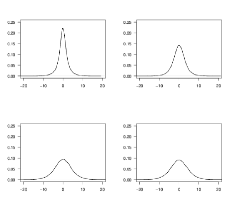
Figure 1: Non-parametric approximations to the integral priors (top, left: receptor; top, right: intercept; bottom, left and right: stage) based on 50,000 iterations of the associated Markov chain.

Figure 1 shows the integral priors for model $M_{2}$. All the priors are centred around zero. In the first row there are the priors for the coefficient of the receptor level and the intercept, the second row corresponds to the stage.

In this example with four regression coefficients and a sample of size $192$, the high posterior probability of model $M_{2}$ indicates that there exists an association between mortality and receptor level, although such probability is not conclusive.

On the other hand, it is well-known that stage is a factor that is strongly related with mortality. We have computed the posterior probability of the full model versus the model that includes the intercept and the receptor level obtaining a posterior probability of $0.999$. This very large value means that we can conclude that the most important predictor is by far the stage if we are looking for a reduced model that satisfactorily explain the data. For comparison, in this case the odds ratios are $3.11$ and $18.84$ and the p-values are $0.01485$ and $5.34e-07$, respectively.

5.2 Low birth weight

The birthwt dataset is made of 189 rows and 10 columns (see the object birthwt from the statistical software R). Data were collected at the Baystate Medical Center, Springfield, Massachusetts in 1986 in order to attempt to identify which factors contributed to an increased risk of low birth-weight babies. Information was recorded from 189 women of whom 59 had low birth-weight infants. We use this dataset and the logistic link function to illustrate further the integral priors methodology.

We first studied the association between the low birth-weight and smoking (two levels), race (three levels), previous premature labours (two levels) and age (five levels, defined by taking the intervals with included upper endpoints $18,20,25,30$ and $\infty$, respectively). We have considered as the reduced model the one without the variable “smoking”. The p-value associated with the exclusion of “smoking” is $0.014$ and the corresponding estimation of the odds ratio is $2.62$.

Figure 2: Non-parametric approximations to the integral prior distributions for model $M_{2}$ associated with the birthwt dataset for the nine regression coefficients.

The analysis is based on $30,000$ iterations of the Markov chain and $10,000$ simulations from the importance sampling density. It yields $0.67$ as the posterior probability that smoking has an effect over the low birth-weight. Figure 2 produces an approximation of the integral prior distributions for the nine regression coefficients. The integral priors for all regression coefficients under model $M_{2}$ are very similar except the one for the smoking coefficient; this prior is more concentrated about the null hypothesis. The standard deviations for those priors are 4.2, 5.4, 5.5, 4.9, 5.7, 5.4, 5.8, 6.2 and 5.1, respectively, showing again that the prior on the smoking coefficient (first standard deviation) is more concentrated about the null hypothesis while the others are similar.

To study the stability of these results, based on $T=10,000$, $20,000$ and $30,000$ iterations, we ran 30 Markov chains of length $T$ and, in parallel, importance sampling with $T$ simulations as well. Mean and standard deviation for the 30 estimations of the posterior probability of the model $M_{2}$ are reported in Table (3).

Table 3: Estimations of the posterior probability of the model $M_{2}$ running 30 Markov chains of length $T$ and importance sampling simulations based on $T$ simulations as well

		$T=10000$		$T=20000$		$T=30000$
Mean		$0.671$		$0.673$		$0.681$
Standard deviation		$0.0143$		$0.014$		$0.010$

6 Conclusions

Integral prior distributions have successfully been constructed towards an objective Bayesian model selection analysis in binomial regression models and the methodology has been applied in two examples with the logistic regression. This analysis has been done within the model selection framework and it remains completely automatic since no other choice than the reference priors for the competing models under consideration is requested. Although unrelated with the purpose of this paper, this methodology can be applied to variable selection problems, using an encompassing structure defined from above or from below as done applying the intrinsic priors methodology in León-Novelo et al. (2012).

Furthermore, for the sake of comparison we have applied the intrinsic prior methodology in León-Novelo et al. (2012) to our examples. For the breast cancer example we have calculated 30 times the posterior probability of the full model using the package varSelectIP that implements the intrinsic priors for the probit model, see León-Novelo et al. (2012). The 30 computed values ranged from 0.607 to 0.809 with a mean of 0.703 and standard deviation 0.055, thus exhibiting a similar answer but with more variability than the integral methodology, see Table (2). For the second example (low birth-weight) the posterior probability of the full model using the package varSelectIP 30 times ranged from 0.820 to 0.922 with a mean of 0.870 and standard deviation 0.024, showing again that the integral methodology is more stable that the one implemented with intrinsic priors (package varSelectIP); at last, the conclusion using integral priors is more conservative, which is a rather positive argument in medical studies when one is trying to associate an exposure with an illness.

This feature could be the consequence of the property that despite the fact that both the integral and the intrinsic priors are centred around the null hypotheses, the corresponding null hypotheses are defined in different ways since, when we use the intrinsic priors methodology developed in León-Novelo et al. (2012), the intrinsic priors for all models under consideration are centred around a null model where all the $\beta^{\prime}s$ are zero except for the intercept, that is the reference model for the intrinsic methodology. Nevertheless, we should keep in mind that computations with integral priors were made for the logistic model while those for intrinsic priors were made for the probit model.

This work straightforward applies to other link functions and can be extended to compare several link functions (non-nested models). All the computations have been programmed in R and are freely available at the web https://webs.um.es/dsm/miwiki/doku.php?id=investigacion.

References

- Berger and Bernardo (1989) Berger, J. O. & Bernardo, J. M. (1989). Estimating a product of means: Bayesian analysis with reference priors. J. Am. Statist. Assoc. 84, 200–207.
- Berger and Pericchi (1996) Berger, J. O. & Pericchi, L. R. (1996). The intrinsic Bayes factor for model selection and prediction. J. Am. Statist. Assoc. 91, 109–122.
- Berger and Pericchi (2004) Berger, J. O. & Pericchi, L. R. (2004). Training samples in objective Bayesian model selection. Ann. Statist. 32, 841–869.
- Bernardo (1979) Bernardo, J. M. (1979). Reference posterior distribution for Bayesian inference. J. R. Statist. Soc. B 41, 113–147.
- Cano et al. (2007a) Cano, J. A., Kessler, M. & Salmerón, D. (2007a). Integral priors for the one way random effects model. Bayesian Anal. 2, 59–68.
- Cano et al. (2007b) Cano, J. A., Kessler, M. & Salmerón, D. (2007b). A synopsis of integral priors for the one way random effects model. Bayesian Statistics 8, 577–582. Oxford University Press.
- Cano and Salmerón (2013) Cano, J. A. & Salmerón, D. (2013). Integral priors and constrained imaginary training samples for nested and non-nested Bayesian model comparison. Bayesian Anal. 8, 361–380.
- Cano et al. (2008) Cano, J. A., Salmerón, D. & Robert, C. P. (2008). Integral equation solutions as prior distributions for Bayesian model selection. Test 17, 493–504.
- Carlin and Chib (1995) Carlin, B. P. & Chib, S. (1995). Bayesian model choice via Markov chain Monte Carlo methods. J. R. Statist. Soc. B 57, 473–484.
- Casella and Moreno (2006) Casella, G. & Moreno, E. (2006). Objective Bayesian variable selection. J. Am. Statist. Assoc. 101, 157–167.
- Casella and Moreno (2009) Casella, G. & Moreno, E. (2009). Assessing robustness of intrinsic tests of independence in two-way contingency tables. J. Am. Statist. Assoc. 104, 1261–1271.
- Chen et al. (2008) Chen, MH., Ibrahim, J. G. & Kim, S. (2008). Properties and implementation of Jeffreys’s Prior in binomial regression models. J. Am. Statist. Assoc. 103, 1659–1664.
- Consonni et al. (2011) Consonni, G., Moreno, E. & Venturini, S. (2011). Testing Hardy-Weinberg equilibrium: an objective Bayesian analysis. Stat. Med. 30, 62–74.
- Gelfand and Smith (1990) Gelfand, A. & Smith, A. F. M. (1990). Sampling-based approaches to calculating marginal densities. J. Am. Statist. Assoc. 85, 398–409.
- Girón et al. (2006) Girón, F. J., Martínez, M. L., Moreno, E. & Torres, F. (2006). Objective testing procedures in linear models: calibration of the p-values. Scand. J. Stat. 33, 765–784.
- Greenland (2004) Greenland, S. (2004). Model-based estimation of relative risks and other epidemiologic measures in studies of common outcomes and in case-control studies. Am. J. Epidemiol. 160, 301–305.
- Hayfield and Racine (2008) Hayfield, T. & Racine, J. S. (2008). Nonparametric econometrics: the np package. J. Stat. Softw. 27, 1–32.
- Ibrahim and Laud (1991) Ibrahim, J. G. & Laud, P. W. (1991). On Bayesian analysis of generalized linear models using Jeffreys’s prior. J. Am. Statist. Assoc. 86, 981–986.
- Jeffreys (1961) Jeffreys, H. (1961). Theory of Probability. Oxford University Press, London.
- León-Novelo et al. (2012) León-Novelo, L., Moreno, E. & Casella, G. (2012). Objective Bayes model selection in probit models. Statist. Med. 31, 353–365.
- Moreno et al. (1998) Moreno, E., Bertolino, F. & Racugno, W. (1998). An intrinsic limiting procedure for model selection and hypothesis testing. J. Am. Statist. Assoc. 93, 1451–1460.
- Moreno and Girón (2006) Moreno, E. & Girón, F. J. (2006). On the frequentist and Bayesian approaches to hypothesis testing (with discussion). Sort 30, 3–54.
- Pérez and Berger (2002) Pérez, J. M. & Berger, J. O. (2002). Expected posterior prior distributions for model selection. Biometrika 89, 491–511.
- Sabanés and Held (2011) Sabanés, D. & Held, L. (2011). Hyper- priors for generalized linear models. Bayesian Anal. 6, 1–24.
- Schwarz (1978) Schwarz, G. (1978). Estimating the dimension of a model. Ann. Statist. 6, 461–464.