Optimal Tx-BF for MIMO SC-FDE Systems

Abstract

Transmit beamforming (Tx-BF) for multiple-input multiple-output (MIMO) channels is an effective means to improve system performance. In frequency-selective channels, Tx-BF can be implemented in combination with single-carrier frequency-domain equalization (SC-FDE) to combat inter-symbol interference. In this paper, we consider the optimal design of the Tx-BF matrix for a MIMO SC-FDE system employing a linear minimum mean square error (MSE) receiver. We formulate the Tx-BF optimization problem as the minimization of a general function of the stream MSEs, subject to a transmit power constraint. The optimal structure of the Tx-BF matrix is obtained in closed form and an efficient algorithm is proposed for computing the optimal power allocation. Our simulation results validate the excellent performance of the proposed scheme in terms of uncoded bit-error rate and achievable bit rate.

I Introduction

Multiple-input multiple-output (MIMO) systems are a promising technology to improve the spectrum efficiency and/or error performance of wireless networks. In order to fully exploit the benefits of the multiple antennas and the available channel state information at the transmitter (CSIT), appropriate MIMO transmit beamforming (Tx-BF) schemes are required. Optimal MIMO Tx-BF designs for flat fading channels and frequency selective fading channels in combination with orthogonal frequency-division multiplexing (OFDM) have been well studied in the literature, cf. [1]-[3]. However, the design methodology used in [1]-[3] is not directly applicable to MIMO systems employing single-carrier frequency-domain equalization (SC-FDE) [4], where a block circular matrix structure is imposed on the equalization matrix to enable efficient frequency domain implementation. In particular, for MIMO SC-FDE systems, the system performance metrics depend on the mean square errors (MSEs) of the spatial data streams in the time domain, instead of the subcarrier MSEs in the frequency domain as is the case for OFDM systems. Tx-BF design for SC-FDE systems has been investigated in several works. For example, adopting the arithmetic MSE (AMSE) as the performance metric, [5] proposed optimal Tx-BF for a MIMO SC-FDE system with both linear and decision feedback equalization. However, obtaining the optimal Tx-BF matrix design directly minimizing the bit-error rate (BER) or maximizing the achievable bit rate (ABR) is much more challenging since, unlike the AMSE, these performance metrics are nonlinear functions of the data stream MSEs. In [6], the authors provide a first attempt to minimize the BER of a multiple-input single-output (MISO) SC-FDE system. However, since only one data stream is transmitted, minimizing the BER is equivalent to minimizing the AMSE for MISO systems. To the best of the author’s knowledge, Tx-BF design for MIMO SC-FDE systems with general non-AMSE based objective functions has not been studied in the literature yet.

In this paper, we propose an optimal Tx-BF design for MIMO SC-FDE systems. After deriving the optimal linear minimum MSE receiver and the associated stream MSEs, we formulate the Tx-BF optimization problem as the minimization of general Schur-convex and Schur-concave functions of the MSEs under a transmit power constraint. To solve the optimization problem, we first obtain the optimal structure of the Tx-BF matrix based on majorization theory. This allows us to transform the original complex matrix problem into a real scalar power optimization problem. Similar to the case of MIMO OFDM, the proof of the optimal structure of the Tx-BF matrix for MIMO SC-FDE is based on the Schur-convexity/concavity of the objective function [2, 7]. However, the power allocation problem for MIMO SC-FDE is quite different from the power allocation problem for MIMO OFDM.

In this paper, $\rm tr({\mathbf{A}})$, ${\mathbf{A}}^{-1}$, ${\mathbf{A}}^{T}$, and ${\mathbf{A}}^{{\dagger}}$ denote the trace, inverse, transpose, and conjugate transpose of matrix ${\mathbf{A}}$, respectively. $\mathbb{C}^{M\times N}$ denotes the space of all complex $M\times N$ matrices and ${\mathbf{I}}_{M}$ is the $M\times M$ identity matrix. ${\mathbf{n}}\sim\mathcal{CN}(\mathbf{0},\sigma_{n}^{2}{\mathbf{I}}_{M})$ indicates that ${\mathbf{n}}\in\mathbb{C}^{M\times 1}$ is a complex Gaussian distributed vector with zero mean and covariance matrix $\sigma_{n}^{2}{\mathbf{I}}_{M}$. $E[\cdot]$ and $\otimes$ denote statistical expectation and the Kronecker product, respectively. $\mbox{blkcirc}([{\mathbf{A}}_{1}^{T},{\mathbf{A}}_{2}^{T},...,{\mathbf{A}}_{M}^{T}]^{T})$ and $\mbox{blkdiag}([{\mathbf{A}}_{1}^{T},{\mathbf{A}}_{2}^{T},...,{\mathbf{A}}_{M}^{T}]^{T})$ denote a block circular matrix and a block diagonal matrix, respectively, formed by the block-wise vector $[{\mathbf{A}}_{1}^{T},{\mathbf{A}}_{2}^{T},...,{\mathbf{A}}_{M}^{T}]^{T}$. $\mathbb{F}\in\mathbb{C}^{N_{c}\times N_{c}}$ denotes the Fast Fourier Transform (FFT) matrix.

II System Model and MSE FDE

II-A System Model

We consider a MIMO SC-FDE system with $N_{t}$ transmit antennas and $N_{r}$ receive antennas, as shown in Fig. 1. Let ${\mathbf{s}}_{n}=[s_{n}(1),s_{n}(2),\ldots,s_{n}(M)]^{T},n=0,...,N_{c}-1,$ denote the symbol vector at time $n$, where $s_{n}(j)$ denotes the $n$th symbol on the $j$th spatial stream and $M\leq\min\{N_{t},N_{r}\}$ is the number of transmitted data streams. The $s_{n}(j)$ are independent and identical distributed with zero mean and variance $\sigma_{s}^{2}$. Stacking all symbol vectors into one vector leads to ${\mathbf{s}}=[{\mathbf{s}}_{0}^{T},\ldots,{\mathbf{s}}_{N_{c}-1}^{T}]^{T}$. Next, ${\mathbf{s}}$ is transformed into the frequency domain (FD) and processed by the FD BF matrix ${\mathbf{P}}_{f}={\rm blkdiag}\{[{\mathbf{P}}_{0}^{T},...,{\mathbf{P}}_{N_{c}-1}^{T}]^{T}\}$, with ${\mathbf{P}}_{k}\in\mathbb{C}^{N_{t}\times M}$ being the BF matrix at frequency $k$. Subsequently, the signal is converted back to the time domain (TD). Then, the signal is prepended by a Cyclic Prefix (CP), which includes the last $N_{t}K$ data symbols ($K\geq L$ and $L$ is the maximum channel impulse response (CIR) length), and sent over the time dispersive channel.

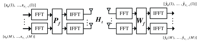
Figure 1: System model for the MIMO SC-FDE system. FFT and IFFT denote the $N_{c}$-point FFT and inverse FFT, respectively.

The CP converts the linear convolution of the CIR and the signal vector to a circular convolution. Hence, after CP removal, the channel matrix seen by the receiver is a block circular matrix ${\mathbf{H}}_{t}={\rm blkcirc}\{[{\mathbf{H}}_{t,0}^{T},...,{\mathbf{H}}_{t,L_{h}-1}^{T},\mathbf{0}_{N_{t}\times N_{r}(N_{c}-L_{h})}]^{T}\}$ where ${\mathbf{H}}_{t,\ell}\in\mathbb{C}^{N_{r}\times N_{t}}$ denotes the spatial channel matrix of the $\ell$th path. Note that the TD channel matrix can be decomposed as ${\mathbf{H}}_{t}={\mathbf{F}}_{N_{r}}^{\dagger}{\mathbf{H}}_{f}{\mathbf{F}}_{N_{t}}$, where ${\mathbf{F}}_{X}=\mathbb{F}\otimes{\mathbf{I}}_{X}$, and ${\mathbf{H}}_{f}={\rm blkdiag}\{[{\mathbf{H}}_{f,0}^{T},...,{\mathbf{H}}_{f,N_{c}-1}^{T}]^{T}\}$ with ${\mathbf{H}}_{f,k}\in\mathbb{C}^{N_{r}\times N_{t}}$ being the FD channel matrix at frequency $k$. The received signal after CP removal is then given by

$${\mathbf{y}}={\mathbf{H}}_{t}{\mathbf{F}}_{N_{t}}^{\dagger}{\mathbf{P}}_{f}{\mathbf{F}}_{M}{\mathbf{s}}+{\mathbf{n}},$$ (1)

where ${\mathbf{n}}=[{\mathbf{n}}_{1}^{T},\ldots,{\mathbf{n}}_{N_{c}}^{T}]^{T}$ is the noise vector with ${\mathbf{n}}_{n}$ denoting the additive white Gaussian noise (AWGN) vector at time $n$. At the receiver, the signal is converted into the FD and processed by the FDE matrix ${\mathbf{W}}_{f}={\rm blkdiag}\{[{\mathbf{W}}_{0}^{T},...,{\mathbf{W}}_{N_{c}-1}^{T}]^{T}\}$, where ${\mathbf{W}}_{k}\in\mathbb{C}^{M\times N_{r}}$ denotes the FDE matrix at frequency $k$. The equalized signal in the TD is thus given by $\hat{\mathbf{y}}={\mathbf{F}}_{M}^{\dagger}{\mathbf{W}}_{f}{\mathbf{F}}_{N_{r}}{\mathbf{y}}$. Then, the error vector at the equalizer output is ${\mathbf{e}}=\hat{\mathbf{y}}-{\mathbf{s}}$, and the corresponding MSE matrix is obtained as

$${\mathbf{E}}=E[{\mathbf{e}}{\mathbf{e}}^{\dagger}]={\mathbf{F}}_{M}^{\dagger}\Big{[}\sigma_{s}^{2}({\mathbf{W}}_{f}{\mathbf{H}}_{f}{\mathbf{P}}_{f}{\mathbf{P}}_{f}^{\dagger}{\mathbf{H}}_{f}^{\dagger}{\mathbf{W}}_{f}^{\dagger}$$ (2)

$$-{\mathbf{W}}_{f}{\mathbf{H}}_{f}{\mathbf{P}}_{f}-{\mathbf{P}}_{f}^{\dagger}{\mathbf{H}}_{f}^{\dagger}{\mathbf{W}}_{f}^{\dagger}+{\mathbf{I}}_{MN_{c}})+\sigma_{n}^{2}({\mathbf{W}}_{f}{\mathbf{W}}_{f}^{\dagger})\Big{]}{\mathbf{F}}_{M}.$$

II-B Optimal Minimum MSE FDE

Based on (2), we can derive the optimal FDE filter ${\mathbf{W}}_{f}$ which minimizes the sum MSE of all spatial streams for a given Tx-BF matrix ${\mathbf{P}}_{f}$. By differentiating ${\rm tr}({\mathbf{E}})$ with respect to (w.r.t.) ${\mathbf{W}}_{f}$ and setting the result to zero, we obtain the optimal minimum MSE FDE filter and the corresponding MSE matrix,

$${\mathbf{W}}_{f} = \sigma_{s}^{2}\mathbf{\Psi}_{f}^{-1}{\mathbf{P}}_{f}^{{\dagger}}{\mathbf{H}}_{f}^{{\dagger}}\quad\mbox{and}\quad{\mathbf{E}}=\sigma_{s}^{2}{\mathbf{F}}_{M}^{\dagger}\mathbf{\Psi}_{f}^{-1}{\mathbf{F}}_{M},$$ (3)

respectively, where $\mathbf{\Psi}_{f}=\frac{\sigma_{s}^{2}}{\sigma_{n}^{2}}{\mathbf{P}}_{f}^{{\dagger}}{\mathbf{H}}_{f}^{{\dagger}}{\mathbf{H}}_{f}{\mathbf{P}}_{f}+{\mathbf{I}}_{MN_{c}}$. The $k$th block diagonal matrix entry of ${\mathbf{W}}_{f}$ is given by ${\mathbf{W}}_{k}=\sigma_{s}^{2}\mathbf{\Psi}_{k}^{-1}{\mathbf{P}}_{k}^{{\dagger}}{\mathbf{H}}_{f,k}^{{\dagger}}$, where $\mathbf{\Psi}_{k}=\frac{\sigma_{s}^{2}}{\sigma_{n}^{2}}{\mathbf{P}}_{k}^{{\dagger}}{\mathbf{H}}_{f,k}^{{\dagger}}{\mathbf{H}}_{f,k}{\mathbf{P}}_{k}+{\mathbf{I}}_{M}$. Note that since MSE matrix ${\mathbf{E}}$ is a block circular matrix, its block diagonal entries are all identical, i.e., ${\mathbf{E}}_{k}=\hat{\mathbf{E}},\forall k$. By exploiting the structure of ${\mathbf{E}}$, $\hat{\mathbf{E}}$ can be expressed as

$$\hat{\mathbf{E}}=\frac{\sigma_{s}^{2}}{N_{c}}\sum_{k=0}^{N_{c}-1}\mathbf{\Psi}_{k}^{-1}.$$ (4)

III Optimal Tx-BF Matrix Design

Now, we are ready to derive the optimal ${\mathbf{P}}_{f}$ such that a general function of the stream MSEs is minimized, under a power constraint on the Tx-BF matrix. Mathematically, the optimization problem is formulated as:

$$\min_{{\rm tr}({\mathbf{P}}_{f}{\mathbf{P}}_{f}^{\dagger})\leq P_{T}}\quad f(\mbox{diag}[\hat{\mathbf{E}}]),$$ (5)

where $P_{T}$ is the power budget for the transmitter, and $\mbox{diag}[{\mathbf{M}}]$ denotes a vector containing the diagonal entries of matrix ${\mathbf{M}}$. The considered objective functions $f(\mbox{diag}[\hat{\mathbf{E}}])$ can be either Schur-convex or Schur-concave functions [2] w.r.t. $\mbox{diag}[\hat{\mathbf{E}}]$.

III-A Optimal Structure of the Tx-BF Matrix

We first investigate the optimal structure of the Tx-BF matrix. We begin by introducing the singular-value decomposition (SVD) of the FD channel matrix

$${\mathbf{H}}_{f,k}={\mathbf{U}}_{H}^{(k)}\mathbf{\Lambda}_{H}^{(k)}{\mathbf{V}}_{H}^{(k){\dagger}},\quad\forall k,$$ (6)

where ${\mathbf{U}}_{H}^{(k)}\in\mathbb{C}^{N_{r}\times N_{r}}$ and ${\mathbf{V}}_{H}^{(k)}\in\mathbb{C}^{N_{t}\times N_{t}}$ are the singular-vector matrices of ${\mathbf{H}}_{f,k}$, and $\mathbf{\Lambda}_{H}^{(k)}\in\mathbb{C}^{N_{r}\times N_{t}}$ is the singular-value matrix of ${\mathbf{H}}_{f,k}$ with increasing diagonal elements.

Theorem 1

For the optimization problem in (5), the following structure of ${\mathbf{P}}_{k}$ is optimal

$${\mathbf{P}}_{k} =\bar{{\mathbf{V}}}_{H}^{(k)}\mathbf{\Lambda}_{P}^{(k)}{\mathbf{V}}_{0},\quad\forall k,$$ (7)

where $\bar{{\mathbf{V}}}_{H}^{(k)}\in\mathbb{C}^{N_{t}\times M}$ contains the $M$ right-most columns of ${{\mathbf{V}}}_{H}^{(k)}$, and $\mathbf{\Lambda}_{P}^{(k)}\in\mathbb{C}^{M\times M}$ is a diagonal matrix with the $m$th diagonal element denoted by $\sqrt{P_{km}}$. For Schur-concave functions, ${\mathbf{V}}_{0}={\mathbf{I}}_{M}$, and for Schur-convex functions, ${\mathbf{V}}_{0}$ is a unitary matrix which makes all diagonal entries of $\hat{\mathbf{E}}$ equal .

Proof:

Please refer to Appendix A. ∎

In the following, we consider some typical objective functions that are based on the stream MSEs, and which have been extensively investigated for MIMO OFDM systems based on the subcarrier MSEs [2]. Specifically, we consider the AMSE, geometric MSE (GMSE), maximum MSE (maxMSE), arithmetic signal-to-interference-plus-noise ratio (ASINR), geometric SINR (GSINR), harmonic SINR (HSINR), and arithmetic bit error rate (ABER) for optimization, i.e.,

$$f^{\rm[X]}(\mbox{diag}[\hat{\mathbf{E}}])=\begin{cases}\begin{array}[]{c}\sum_{m=1}^{M}\hat{\mathbf{E}}_{mm},\quad\mbox{X=AMSE}\\ \prod_{m=1}^{M}\hat{\mathbf{E}}_{mm},\quad\mbox{X=GMSE}\\ \max_{m=1}^{M}\hat{\mathbf{E}}_{mm},\quad\mbox{X=maxMSE}\\ -\sum_{m=1}^{M}\left(\hat{\mathbf{E}}_{mm}^{-1}-1\right),\quad\mbox{X=ASINR}\\ -\prod_{m=1}^{M}\left(\hat{\mathbf{E}}_{mm}^{-1}-1\right),\quad\mbox{X=GSINR}\\ \sum_{m=1}^{M}\left(\hat{\mathbf{E}}_{mm}^{-1}-1\right)^{-1},\quad\mbox{X=HSINR}\\ \sum_{m=1}^{M}\alpha Q\left(\sqrt{\beta(\hat{\mathbf{E}}_{mm}^{-1}-1)}\right),\mbox{X=ABER}\\ \end{array}\end{cases}$$

where $\hat{\mathbf{E}}_{mm}$ is the $m$th diagonal entry of $\hat{\mathbf{E}}$, $Q(\cdot)$ is the Gaussian $Q$-function, and $\alpha$ and $\beta$ are constellation dependent coefficients. Here, we assume all streams adopt the same signal constellation. Note that the objective functions for the AMSE, GMSE, ASINR, and GSINR criteria are Schur-concave functions, while those for the maxMSE, HSINR, and ABER criteria are Schur-convex functions w.r.t. $\mbox{diag}[\hat{\mathbf{E}}]$ [2].

Exploiting the optimal structure of the Tx-BF matrix in (7), we can express $\mathbf{\Psi}_{k}$ as $\mathbf{\Psi}_{k}={\mathbf{V}}_{0}^{\dagger}\mathbf{\hat{\Psi}}_{k}{\mathbf{V}}_{0}$, with $\mathbf{\hat{\Psi}}_{k}=\frac{\sigma_{s}^{2}}{\sigma_{n}^{2}}\mathbf{\Lambda}_{P}^{(k){\dagger}}\bar{\mathbf{\Lambda}}_{H}^{(k){\dagger}}\bar{\mathbf{\Lambda}}_{H}^{(k)}\mathbf{\Lambda}_{P}^{(k)}+{\mathbf{I}}_{M}$, where $\bar{\mathbf{\Lambda}}_{H}^{(k)}=\mbox{diag}[\sqrt{H_{km}}]$ contains the $M$ largest diagonal entries of $\mathbf{\Lambda}_{H}^{(k)}$. Now, we can write the MSE matrix as $\hat{\mathbf{E}}=\frac{\sigma_{s}^{2}}{N_{c}}\sum_{k=0}^{N_{c}-1}\mathbf{\hat{\Psi}}_{k}^{-1}$, where the diagonal entries of $\mathbf{\hat{\Psi}}_{k}$ are given by ${\Psi}_{km}=\frac{\sigma_{s}^{2}}{\sigma_{n}^{2}}P_{km}H_{km}+1,\forall m$.

Proposition 1: The optimization problems in (5) with Schur-convex objective functions, i.e., maxMSE, HSINR, and ABER, are equivalent to AMSE minimization up to a unitary rotation of the Tx-BF.

Proof:

For Schur-convex functions, the unitary rotation matrix ${\mathbf{V}}_{0}$ has to make all stream MSEs identical, e.g., equal to $\hat{E}$. Explicitly, we can write $\hat{E}={\rm tr}(\hat{\mathbf{E}})/M=\frac{\sigma_{s}^{2}}{MN_{c}}{\rm tr}(\sum_{k=1}^{N_{c}}\mathbf{\hat{\Psi}}^{-1}_{k})=\frac{\sigma_{s}^{2}}{MN_{c}}\sum_{k=1}^{N_{c}}\sum_{m=1}^{M}{\Psi}_{km}^{-1}$, which is essentially the objective function for the AMSE criterion. On the other hand, as the Schur-convex objective functions are monotonically increasing w.r.t. $\hat{E}$, the corresponding problems are equivalent to AMSE minimization up to a unitary rotation (as the AMSE objective function is Schur-concave). ∎

Remark 1: For MIMO OFDM systems, optimization problems employing different Schur-convex functions are not equivalent [2], since in this case, the unitary matrix only balances the MSEs on each subcarrier, while the MSEs across the subcarriers are not identical.

Now, we can restate the objective functions in terms of the new variables ${\mathbf{P}}=\{P_{km},\forall k,m\}$ as $f^{\rm[X]}({\mathbf{P}})=\sum_{m=1}^{M}f_{m}^{\rm[X]}({\mathbf{P}})$ with

$$f^{\rm[X]}_{m}({\mathbf{P}})=\begin{cases}\begin{array}[]{c}\frac{\sigma_{s}^{2}}{N_{c}}\sum_{k=0}^{N_{c}-1}{\Psi}_{km}^{-1},\quad\mbox{X=AMSE}\\ \log_{2}\Big{(}\frac{\sigma_{s}^{2}}{N_{c}}\sum_{k=0}^{N_{c}-1}{\Psi}^{-1}_{km}\Big{)},\quad\mbox{X=GMSE}\\ -\Big{(}\frac{\sigma_{s}^{2}}{N_{c}}\sum_{k=0}^{N_{c}-1}{\Psi}^{-1}_{km}\Big{)}^{-1},\quad\mbox{X=ASINR}\\ -\log_{2}\left(\Big{[}\frac{\sigma_{s}^{2}}{N_{c}}\sum_{k=0}^{N_{c}-1}{\Psi}^{-1}_{km}\Big{]}^{-1}-1\right),\mbox{X=GSINR}\end{array}\end{cases}$$

where for GMSE and GSINR, we have taken the logarithm of the original objective functions to facilitate the subsequent optimization. Furthermore, we have omitted the objective functions for the maxMSE, HSINR, and ABER criteria since they yield the same power allocation as the AMSE criterion, cf. Proposition 1.

III-B Optimal Power Allocation for the Tx-BF Matrix

Using Theorem 1, the power constraint can be expressed as $\sum_{k=0}^{N_{c}-1}\sum_{m=1}^{M}P_{km}\leq P_{T}$. The problem is then reformulated as

$$\min_{\sum_{k=0}^{N_{c}-1}\sum_{m=1}^{M}P_{km}\leq P_{T}} f^{\rm[X]}\left({\mathbf{P}}\right).$$ (8)

Proposition 2: The considered objective functions $f^{\rm[X]}({\mathbf{P}}),{\rm X}=\{\rm AMSE,GMSE,ASINR,GSINR\}$, are all convex functions w.r.t. $P_{km}$.

Proof:

Please refer to Appendix B. ∎

The convexity of the problem in (8) guarantees the existence of a global optimum solution for the power allocation. In addition, since the power constraint is affine and feasible, the Slater condition is satisfied [8], implying that strong duality holds. This allows us to solve the original primal problem by solving its dual problem. To this end, we first write the Lagrangian of (8) as $\mathcal{L}=\sum_{m=1}^{M}\left(f^{\rm[X]}_{m}({\mathbf{P}})+\lambda\sum_{k=0}^{N_{c}-1}P_{km}\right)-\lambda P_{T}$, where $\lambda$ is the Lagrange multiplier for the constraint in (8). The corresponding dual problem can be written as

$$\max_{\lambda\geq 0}~{}~{}\min_{\{P_{km}\geq 0\}}~{}~{}\mathcal{L}.$$ (9)

For a given $\lambda$, the inner minimization problem in (9) can be solved by applying the Karush-Kuhn-Tucker conditions [8]. The optimal solution for $P_{km}$ is found as

$$P_{km}=\left(\sqrt{\frac{\sigma_{n}^{2}B_{m}}{\sigma_{s}^{2}\lambda H_{km}}}-\frac{\sigma_{n}^{2}}{\sigma_{s}^{2}H_{km}}\right)^{+},$$ (10)

where $B_{m}$ is a factor that depends on the objective functions,

$$B_{m}=\begin{cases}\begin{array}[]{c}1,\quad\mbox{X=AMSE}\\ (\frac{\sigma_{s}^{2}\ln 2}{N_{c}}\sum_{k=0}^{N_{c}-1}{\Psi}^{-1}_{km})^{-1},\quad\mbox{X=GMSE}\\ (\frac{\sigma_{s}^{2}}{N_{c}}\sum_{k=0}^{N_{c}-1}{\Psi}^{-1}_{km})^{-2},\quad\mbox{X=ASINR}\\ \frac{C_{m}}{\ln 2}(\frac{\sigma_{s}^{2}}{N_{c}}\sum_{k=0}^{N_{c}-1}{\Psi}^{-1}_{km})^{-2},\quad\mbox{X=GSINR}\\ \end{array}\end{cases}$$ (11)

with $C_{m}=\left(\Big{[}\frac{\sigma_{s}^{2}}{N_{c}}\sum_{k=0}^{N_{c}-1}{\Psi}^{-1}_{km}\Big{]}^{-1}-1\right)^{-1}$.

Remark 2: Recall that for MIMO OFDM systems [2], the Tx-BF optimization based on the GSINR criterion leads to equal power allocation, the ASINR criterion leads to allocating all the transmit power to the strongest spatial stream among all the subcarriers, and for Schur-convex functions, different multilevel waterfilling solutions are needed. In contrast, for MIMO SC-FDE systems, the solutions for all criteria exhibit a simple single-level waterfilling structure, cf. (10).

For the outer maximization problem in (9), we can obtain the optimal Lagrange multiplier $\lambda$ by using the iterative subgradient method [8]

$$\lambda^{[i+1]}=\left[\lambda^{[i]}-\varepsilon^{[i+1]}\left(\sum_{k=0}^{N_{c}-1}\sum_{m=1}^{M}P_{km}^{[i]}-P_{T}\right)\right]^{+},$$ (12)

where $\varepsilon^{[i]}$ is the step size adopted in the $i$th iteration, $\lambda^{[i]}$ is the Lagrange multiplier obtained in the $i$th iteration and $P_{km}^{[i]}$ is the solution of (10) for a given $\lambda^{[i]}$. For a nonsummable diminishing step size, i.e., $\lim_{i\rightarrow\infty}\varepsilon^{[i]}=0$, $\sum_{i=1}^{\infty}\varepsilon^{[i]}=\infty$, the subgradient method is guaranteed to converge to the optimal dual variable $\lambda$ [9]. The optimal primal variables $P_{km}$ can then be obtained from (10).

IV Simulation Results

In this section, we evaluate the performance of the proposed Tx-BF schemes for MIMO SC-FDE using simulations. Each data block contains $N_{c}=64$ symbols. The channel vectors are modeled as uncorrelated Rayleigh block fading channels with power delay profile [10] $p[n]=\frac{1}{\sigma_{t}}\sum_{l=0}^{L-1}e^{-n/\sigma_{t}}\delta[n-l]$, where $\sigma_{t}=2$, which corresponds to moderate frequency-selective fading. For convenience, we assume $L$ and $K$ are both equal to 16. The number of spatial data streams and the number of transmit and receive antennas are all set to be two, i.e., $M=N_{t}=N_{r}=2$. The signal to noise ratio is defined as $SNR=\frac{\sigma_{s}^{2}P_{T}}{MN_{c}\sigma_{n}^{2}}$. All simulations are averaged over at least 100,000 independent channel realizations and data blocks.

In Fig. 2, we show the uncoded BER of a MIMO SC-FDE system with quaternary phase shift keying (QPSK) transmission using different optimization criteria. For comparison, the BER of a MIMO SC-FDE system with equal power allocation (EPA) and the BERs of optimized MIMO OFDM systems are also shown. As can be seen, MIMO SC-FDE achieves a much lower BER than its OFDM counterpart since SC-FDE can exploit the frequency-diversity of the channel. Similar to MIMO OFDM, SC-FDE systems optimized for Schur-convex functions perform better than those optimized for Schur-concave functions. For SC-FDE systems, all Schur-convex objective functions lead to the same BER, which is much lower than that for the Schur-concave AMSE criterion although they use identical power allocations.

In Fig. 3, we show the average achievable bit rate (ABR) of MIMO SC-FDE employing the proposed Tx-BF scheme. The corresponding ABR of an optimized MIMO OFDM system are also shown for reference. For both systems, we have assumed perfect channel loading with continuous constellation size and optimal channel coding [4]. From the figure, we observe that the GMSE criterion achieves the highest ABR and GSINR only suffers from a small ABR loss in the low SNR regime compared to GMSE. In fact, it is straightforward to show that GMSE minimization is equivalent to ABR maximization. The SNR gap between the best SC-FDE and OFDM ABR curves is around 1 dB. Different from OFDM, for SC-FDE, the systems optimized for Schur-convex functions achieve the same ABRs as the system optimized for the AMSE criterion, which implies that the unitary rotation matrix ${\mathbf{V}}_{0}$ does not affect the ABR performance. Furthermore, for the maxMSE and ABER criteria, SC-FDE systems achieve much higher ABRs than OFDM systems, as the latter allocate most of the available power to weaker subcarriers to balance the MSE/BER, and thus compromise the system ABR.

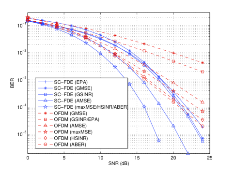
Figure 2: BER comparison of the optimized MIMO SC-FDE and MIMO OFDM systems.

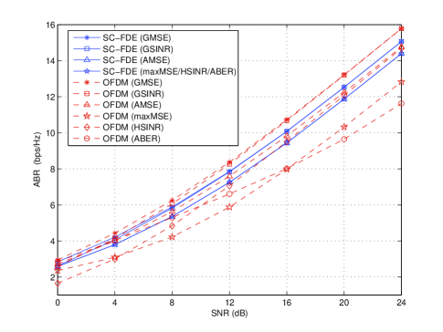
Figure 3: ABR comparison of the optimized MIMO SC-FDE and MIMO OFDM systems.

V Conclusion

In this paper, we addressed the problem of Tx-BF matrix design for MIMO SC-FDE systems. The optimal minimum MSE FDE filter was derived first, along with the stream MSEs at the equalizer output. Then, we optimized the Tx-BF matrix for minimization of a general function of the stream MSEs. We found the optimal structure of the Tx-BF matrix in closed form and proposed an efficient algorithm to solve the remaining power allocation problem. Our results show that AMSE based Tx-BF optimization [5, 6] is neither optimal for minimizing the uncoded BER nor for maximizing the achievable bit rate of MIMO SC-FDE systems.

Appendix A

For Schur-concave functions, from majorization theory [7, 9.B.1], we have $f({\rm diag}(\hat{\mathbf{E}}))\geq f({\rm eig}(\hat{\mathbf{E}}))$, where ${\rm eig}(\hat{\mathbf{E}})$ is a vector containing the eigenvalues of $\hat{\mathbf{E}}$ sorted in decreasing order and equality is achieved if $\hat{\mathbf{E}}$ is a diagonal matrix. From (4), a sufficient condition to achieve this objective function lower bound is to make $\mathbf{\Psi}_{k}^{-1},\forall k,$ diagonal, i.e., ${\mathbf{P}}_{k}^{\dagger}{\mathbf{H}}_{f,k}^{\dagger}{\mathbf{H}}_{f,k}{\mathbf{P}}_{k}={\mathbf{D}}_{k}\in\mathbb{C}^{M\times M}$ is a diagonal matrix with increasing diagonal entries. For subsequent use, we write ${\mathbf{H}}_{f,k}{\mathbf{P}}_{k}={\mathbf{Q}}_{k}{\mathbf{D}}_{k}^{1/2}$, where ${\mathbf{Q}}_{k}\in\mathbb{C}^{N_{t}\times M}$ is a unitary matrix, and ${\mathbf{D}}_{k}^{1/2}$ is the square root of ${\mathbf{D}}_{k}$. Now, we derive the optimal ${\mathbf{P}}_{k}$ that minimizes the transmit power. For notational simplicity, we only consider the case when ${\rm rank}({\mathbf{H}}_{f,k})=N_{t}=N_{r},\forall k$. Using the SVD of ${\mathbf{H}}_{f,k}$, we can rewrite ${\mathbf{P}}_{k}$ as ${\mathbf{P}}_{k}={\mathbf{V}}_{H}^{(k)}\mathbf{\Lambda}_{H}^{(k)-1}{\mathbf{U}}_{H}^{(k){\dagger}}{\mathbf{Q}}_{k}{\mathbf{D}}_{k}^{1/2}$. The power consumption at frequency $k$ is thus given by ${\rm tr}({\mathbf{P}}_{k}{\mathbf{P}}_{k}^{\dagger})={\rm tr}(\mathbf{\Lambda}_{H}^{(k)-2}{\mathbf{T}}_{k}{\mathbf{D}}_{k}{\mathbf{T}}_{k}^{\dagger})\geq{\rm tr}(\mathbf{\bar{\Lambda}}_{H}^{(k)-2}{\mathbf{D}}_{k})$, where $\mathbf{\bar{\Lambda}}_{H}^{(k)}$ is a diagonal matrix containing the $M$ largest singular values of $\mathbf{\Lambda}_{H}^{(k)}$, ${\mathbf{T}}_{k}={\mathbf{U}}_{H}^{(k){\dagger}}{\mathbf{Q}}_{k}$, and the inequality is due to [7, 9.H.1]. Since equality is achieved if ${\mathbf{T}}_{k}=[\mathbf{0}_{M\times(N_{T}-M)}\quad{\mathbf{I}}_{M}]^{T}$, we obtain ${\mathbf{Q}}_{k}=\bar{\mathbf{U}}_{H}^{(k)}$, where $\bar{\mathbf{U}}_{H}^{(k)}$ contains the $M$ right-most columns of ${\mathbf{U}}_{H}^{(k)}$. Plugging ${\mathbf{Q}}_{k}=\bar{\mathbf{U}}_{H}^{(k)}$ into the expression for ${\mathbf{P}}_{k}$, we obtain the optimal ${\mathbf{P}}_{k}$ as ${\mathbf{P}}_{k}=\bar{\mathbf{V}}_{H}^{(k)}\mathbf{\Lambda}_{P}^{(k)}$ where $\bar{\mathbf{V}}_{H}^{(k)}$ contains the $M$ right-most columns of ${\mathbf{V}}_{H}^{(k)}$, and $\mathbf{\Lambda}_{P}^{(k)}=\mathbf{\bar{\Lambda}}_{H}^{(k)-1}\mathbf{{\mathbf{D}}}_{k}^{1/2}$.

For Schur-convex objective functions, from [7, p.7], we have $f({\rm diag}(\hat{\mathbf{E}}))\geq f({\rm tr}(\hat{\mathbf{E}})\mathbf{1}/M)$, where $\mathbf{1}$ is the all-one vector, and equality is achieved if $\hat{\mathbf{E}}$ has identical diagonal entries equal to ${\rm tr}(\hat{\mathbf{E}})/M$. Denote the eigenvalue decomposition of $\hat{\mathbf{E}}(\{{\mathbf{P}}_{k}\})$ for a feasible ${\mathbf{P}}_{k}$ as $\hat{\mathbf{E}}(\{{\mathbf{P}}_{k}\})={\mathbf{U}}_{E}^{\dagger}\mathbf{\Lambda}_{E}{\mathbf{U}}_{E}$. Now consider another feasible Tx-BF matrix $\tilde{\mathbf{P}}_{k}={\mathbf{P}}_{k}{\mathbf{U}}_{E}{\mathbf{V}}_{0}$, where ${\mathbf{V}}_{0}$ is a unitary matrix. Then, we have $\hat{\mathbf{E}}(\{\tilde{\mathbf{P}}_{k}\})={\mathbf{V}}_{0}^{\dagger}\mathbf{\Lambda}_{E}{\mathbf{V}}_{0}$ and according to [7, 9.B.2], we can always find a ${\mathbf{V}}_{0}$ such that $\hat{\mathbf{E}}(\{\tilde{\mathbf{P}}_{k}\})$ has identical diagonal entries which equal ${\rm tr}(\hat{\mathbf{E}}(\{\tilde{\mathbf{P}}_{k}\})/M)$. Since $f({\rm diag}[{\rm tr}(\hat{\mathbf{E}})\mathbf{1}/M])$ is monotonic with respect to its argument, the remaining task is to minimize ${\rm tr}(\hat{\mathbf{E}})$, which is a Schur-concave function. Since for Schur-concave function, the optimal ${\mathbf{P}}_{k}$ diagonalizes $\hat{\mathbf{E}}$, we have ${\mathbf{U}}_{E}={\mathbf{I}}_{M}$. The optimal Tx-BF matrix for Schur-convex objective functions can then be obtained as $\tilde{\mathbf{P}}_{k}={\mathbf{P}}_{k}{\mathbf{V}}_{0}=\bar{\mathbf{V}}_{H}^{(k)}\mathbf{\Lambda}_{P}^{(k)}{\mathbf{V}}_{0}$. This completes the proof.

Appendix B

For the AMSE criterion, the second order derivatives of the objective function are given by $\frac{\partial^{2}f_{m}^{\rm[AMSE]}({\mathbf{P}})}{\partial P_{km}^{2}}=2{\Psi}^{-3}_{km}H_{km}^{2}\geq 0$ and $\frac{\partial^{2}f_{m}^{\rm[AMSE]}({\mathbf{P}})}{\partial P_{km}P_{jm}}=0,\forall j\neq k$. Therefore, the Hessian matrix is a diagonal matrix with non-negative diagonal entries, which implies that $f_{m}^{\rm[AMSE]}({\mathbf{P}})$ is a convex function w.r.t. $P_{km},\forall k,m$. For the GMSE criterion, we rewrite the objective function as $f_{m}^{\rm[GMSE]}({\mathbf{P}})=\log_{2}\Big{(}\frac{\sigma_{s}^{2}}{N_{c}}\sum_{k=0}^{N_{c}-1}\exp(-\log{\Psi}_{km})\Big{)}$, since $-\log{\Psi}_{km}$ is a convex function, and $\log_{2}\Big{(}\frac{\sigma_{s}^{2}}{N_{c}}\sum_{k=0}^{N_{c}-1}\exp y\Big{)}$ is a convex increasing function w.r.t. $y$ [8], the composition of the two, i.e., $f_{m}^{\rm[GMSE]}({\mathbf{P}})$, is also a convex function w.r.t. $P_{km},\forall k,m$. For the SINR related criteria, it can be shown that the Hessian matrix of the stream SINR, i.e., $(\frac{1}{N_{c}}\sum_{k=0}^{N_{c}-1}{\Psi}_{km}^{-1})^{-1}-1$, is negative semidefinite. Hence, the stream SINRs are concave functions w.r.t. $P_{km},\forall k,m$. Based on this concavity, it is straightforward to show that the objective functions for ASINR and GSINR maximization are convex functions w.r.t. $P_{km},\forall k,m$.

References

- [1] A. Scaglione, P. Stoica, S. Barbarossa, G. B. Giannakis, and H. Sampath, “Optimal designs for space-time linear precoders and decoders,” IEEE Trans. Signal Process., vol. 50, no. 5, pp. 1051-1064. May. 2002.
- [2] D. P. Palomar, J. M. Cioffi, and M. A. Lagunas, “Joint Tx-Rx beamforming design for multicarrier MIMO channels: a unified framework for convex optimization,” IEEE Trans. Signal Process., vol. 51, no. 9, pp. 2381-2401, Sept. 2003.
- [3] D. P. Palomar, and Y. Jiang. “MIMO transceiver design via majorization theory.” Foundations and Trends in Communications and Information Theory, vol. 3, no. 4, pp. 331-551, 2006
- [4] N. Benvenuto and S. Tomasin, “On the comparison between OFDM and single carrier modulation with a DFE using a frequency-domain feedforward filter,” IEEE Trans. Commun., vol. 50, no. 6, pp. 947-955, Jun. 2002.
- [5] U. Dang, M. Ruder, R. Schober, W. Gerstacker, “MMSE beamforming for SC-FDMA transmission over MIMO ISI channels,” EURASIP Journal on Advances in Signal Processing, vol. 2011.
- [6] Q. Huang, M. Ghogho, Y. Li, D. Ma, J. Wei , “Transmit beamforming for MISO frequency-selective channels with per-antenna power constraint and limited-Rate feedback,”, IEEE Trans. Vehicle Technology, vol. 60, no. 6, pp. 3726-3735, Oct. 2011.
- [7] A. W. Marshall, I. Olkin, and B. Arnold, Inequalities: theory of majorization and its applications. New York: Academic, 1979.
- [8] S. Boyd and L. Vandenberghe, Convex Optimization. Cambridge, U.K.: Cambridge Univ. Press, 2004.
- [9] S. Boyd, L. Xiao, and A. Mutapcic, “Subgradient methods,” lecture notes of EE392o, Stanford University, Autumn Quarter 2003-2004.
- [10] T. S. Rappaport, Wireless Communications: Principles and Practice. Prentice Hall, 2002.