Direct evidence for a Coulombic phase in monopole-suppressed SU(2) lattice gauge theory

Abstract

Further evidence is presented for the existence of a non-confining phase at weak coupling in SU(2) lattice gauge theory. Using Monte Carlo simulations with the standard Wilson action, gauge-invariant SO(3)-Z2 monopoles, which are strong-coupling lattice artifacts, have been seen to undergo a percolation transition exactly at the phase transition previously seen using Coulomb-gauge methods, with an infinite lattice critical point near $\beta=3.2$. The theory with both Z2 vortices and monopoles and SO(3)-Z2 monopoles eliminated is simulated in the strong coupling ($\beta=0$) limit on lattices up to $60^{4}$. Here, as in the high-$\beta$ phase of the Wilson action theory, finite size scaling shows it spontaneously breaks the remnant symmetry left over after Coulomb gauge fixing. Such a symmetry breaking precludes the potential from having a linear term. The monopole restriction appears to prevent the transition to a confining phase at any $\beta$. Direct measurement of the instantaneous Coulomb potential shows a Coulombic form with moderately running coupling possibly approaching an infrared fixed point of $\alpha\sim 1.4$. The Coulomb potential is measured to 50 lattice spacings and 2 fm. A short-distance fit to the 2-loop perturbative potential is used to set the scale. High precision at such long distances is made possible through the use of open boundary conditions, which was previously found to cut random and systematic errors of the Coulomb gauge fixing procedure dramatically. The Coulomb potential agrees with the gauge-invariant interquark potential measured with smeared Wilson loops on periodic lattices as far as the latter can be practically measured with similar statistics data.

PACS:11.15.Ha, 11.30.Qc. keywords: lattice gauge theory, confinement, lattice monopoles

1 Introduction

Transforming lattice configurations to the minimal Coulomb gauge allows the definition of a local order parameter for lattice gauge theory, the Coulomb magnetization, which is simply the expectation value of the three-space average of the fourth-direction pointing link. This quantity is defined on spacelike hyperlayers because there is a separate SU(2) global remnant symmetry left on each hyperlayer after Coulomb gauge fixing, so there is technically one order parameter per hyperlayer. Spontaneous breaking of this order parameter can occur and has been seen to occur in Monte Carlo simulations of SU(2) lattice gauge theory at weak coupling[1]. This result appears to hold also on the infinite lattice as determined by standard finite size scaling methods such as Binder cumulant crossings and scaling collapse fits. The infinite lattice critical point was reported as $\beta_{c}=3.18\pm 0.08$. Ref. [1] also shows that this transition is connected to the well known magnetic phase transition in the 3-d O(4) Heisenberg model, through extending the coupling space to one in which vertical plaquettes (those with one timelike link) and horizontal plaquettes (purely spacelike) have different couplings. Such a connection, along with the symmetry-breaking nature of the phase transition makes the usually assumed non-existence of such a phase transition paradoxical. A proof of the existence of this phase transition on the infinite lattice, based on its connection to the Heisenberg model, is given in Ref. [2]. In the Coulomb Gauge, where a local order parameter can be defined, the lattice gauge theory appears to be behaving much like its cousin spin model, having a ferromagnetic phase at weak coupling (analogous to low temperature for the magnetic analogue).

However, the existence of such a phase transition requires giving up a long-standing assumption that the non-abelian lattice gauge theories confine in the continuum limit. This is because it has been shown that spontaneous breaking of the remnant gauge symmetry necessarily leads to a non-confining instantaneous Coulomb potential. Since this potential is an upper limit to the standard interquark potential that also cannot be confining[3, 4]. Although this means that to show non-confinement, demonstration of remnant symmetry breaking is sufficient, it would be interesting to see what the potential actually looks like in the weak-coupling phase, especially outside the perturbative region. In particular it would be very interesting to see whether the running coupling continues to increase or approaches an infrared fixed point. There is a severe difficulty in this program, however, due to the observed Wilson-action critical point being around $\beta=3.2$, because the lattice spacing at say $\beta=3.3$ is likely to be so small as to make it impossible to see the interesting region of 0.5 to 1 fm on practically-sized lattices, for which the temperature will also be too high. So one is motivated to seek actions that will keep the system in the non-confining phase but allow for a larger lattice spacing. If one knew what lattice artifacts were causing the transition to confinement then an action which prohibits these objects could be constructed. $\beta$ could then be lowered to increase the lattice spacing without inducing the phase transition. For instance, in the U(1) theory, abelian monopoles multiply as the coupling is increased eventually forming percolating chains which induces a phase transition to a confining phase[5]. However, if a restriction is placed on the action giving such monopoles an infinite chemical potential, this theory remains in the Coulombic phase for all $\beta$ because the lattice artifacts that cause confinement have been removed [6]. The monopoles could also be removed with a simple plaquette restriction, $p>0.5$, where $p$ is the plaquette variable. Since the continuum limit is defined in the neighborhood of $p=1$, such a restriction does not affect the continuum limit or weak-coupling scaling of the theory. Any objects that can be removed by a plaquette restriction $p>c$ with $c<1$ can be considered strong-coupling lattice artifacts which will not be operating in the continuum limit.

The plan of this paper is to attempt the same program in the SU(2) theory, hypothesizing that confinement here is also due to lattice artifacts which do not survive the continuum limit and can therefore be eliminated without affecting the continuum limit. Whether or not the Coulomb magnetization shows spontaneous symmetry breaking in the infinite lattice limit will be the test of whether a formulation is in the Coulombic or confining phase. A secondary test will be measurement of the instantaneous Coulomb potential itself and also the standard interquark potential, the latter for which no gauge fixing is necessary.

We find that two artifacts must be controlled in order to prevent a transition to confinement, Z2 strings (and their associated monopoles), and SO(3)-Z2 monopoles which are topologically nontrivial realizations of the non-abelian Bianchi identity. The latter are gauge-invariant monopoles first introduced in [7]. To demonstrate the connection of SO(3)-Z2 monopoles to confinement, they were monitored in standard Wilson action simulations (with no gauge fixing) as $\beta$ was increased in the $\beta$-region where the Coulomb magnetization transition was observed[2]. The monopoles were found to form a percolating cluster just beyond $\beta=3.2$. Extrapolating the percolation transition to the infinite lattice gave a $\beta$-value precisely matching the previously identified critical point. The monopoles percolate in the confining phase. This very sharp transition may be used to locate the critical point with high precision. Below, simulations which prohibit SO(3)-Z2 monopoles and also have a plaquette restriction $p>0.01$ are shown. Finite size scaling of the Coulomb magnetization measured in configurations transformed to the minimal Coulomb gauge, shows the system to remain in the spontaneously broken phase on the infinite lattice, even as $\beta\rightarrow 0$. The positive plaquette restriction is needed to eliminate Z2 strings, another lattice artifact known to be able to induce confinement.

The instantaneous Coulomb potential, which is determined from the Coulomb magnetization correlation function, is then measured for this action at $\beta=0$ (the strong coupling limit), as is the standard interquark potential using a conventional smeared Wilson loop approach. The Coulomb potential is known to be an upper limit for the interquark potential (it doesn’t fully incorporate the non-linearities of the gluon self-interaction in the quark color fields)[3]. Unlike the situation for the standard Wilson action in the confining phase, where the Coulomb potential (and force) considerably exceeds the interquark potential (and associated force)[3, 8], here they appear to closely agree. However, even using smeared loops, without extremely high statistics the interquark potential is limited by random error beyond about $R/a=20$ (since the force is smaller here than in the confining phase it is harder to measure in this system at the same lattice spacing). In contrast the Coulomb potential can be measured out to $R/a=50$ even with relatively modest resources. Although the Coulomb potential does not provide a direct measurement of the force between quarks, it still provides a perfectly reasonable definition of the running coupling, which has the additional advantage of renormalization scheme independence[3]. At small distances agreement with the two-loop perturbative running coupling is good, which allows measuring the physical lattice spacing by relating it to the $\Lambda$-parameter. These potentials definitely differ from those of the confining phase when scaled to equal lattice spacings. The monopole-suppressed simulations show a Coulombic behavior with running coupling $\alpha_{s}(R)$ at first consistent with the two-loop form but then slowing down, running approximately linearly up to about 1 fm, and possibly flattening out at a value of around 1.4 at distances beyond 1.3 fm, suggestive of an infrared fixed point. This potential differs greatly from the linear + Coulomb form seen with the straight Wilson action in the confining phase.

Although the previous observation of spontaneous breaking of the remnant symmetry showed that both the weak coupling Wilson-action theory and the SO(3)-Z2 monopole-suppressed theory for all couplings were in a non-confining phase, observation of a Coulombic form for the potential at distances of order 1 fm shows more directly that this non-confining phase exists and can be studied using lattice methods at hadronically interesting length scales. Because all that has been done is elimination of lattice artifacts, this must be the phase of the continuum limit. Therefore, one may have to look beyond gluons, to light quarks and the chirally broken vacuum for the source of confinement.

2 Gauge invariant SO(3) monopoles

We start with Wilson-action SU(2) lattice gauge theory with a positive-plaquette constraint, the positive-plaquette model[9]. This constraint eliminates Z2 strings (strings of negative plaquettes). Z2 strings are responsible for confinement in Z2 lattice gauge theory, so eliminating them causes the Z2 theory to deconfine. The positive-plaquette SU(2) model, however, still confines at small $\beta$ [10]. So in SU(2) there must be something besides Z2 strings that causes confinement. Actually Z2 strings probably are responsible for confinement in the mixed fundamental-adjoint [11] version of SU(2) in the large $\beta_{A}$ region, which includes the Z2 theory as a limiting case. Because Z2 strings can cause confinement (though they are not the only cause) a positive plaquette constraint must be maintained along with any monopole constraint in order to get a possibly non-confined theory. In practice we modify this constraint to $p>0.01$, because although $p>0$ appears to work, some instability leading to larger statistical errors is seen for that case, perhaps because one is right on the edge of a transition. (A short run with a $p>-0.1$ restriction together with the monopole restriction detailed below showed a definite lack of remnant symmetry breaking, signaling confinement).

The identification of the monopole starts with the non-abelian Bianchi identity[12, 13].

Figure 1: Covariant plaquettes and bent double-plaquettes for the lattice non-abelian Bianchi identity.

This can be expressed by first constructing the covariant (untraced) plaquettes that comprise the six faces of an elementary cube, with the necessary “tails” to bring them to the same starting site (Fig. 1). Call these $A$, $B$, $C$, $D$, $E$, and $F$. Now construct three bent double plaquettes also shown in Fig. 1, $X=AB$, $Y=CD$, and $Z=EF$. If one forms the product $XYZ$, each link will exactly cancel with its conjugate, so $XYZ=\mathds{1}$, the unit matrix. This is the non-abelian Bianchi identity. Although the plaquettes are all positive (due to the positive plaquette constraint), and thus have a trivial Z2 component of unity, the double plaquettes may be negative. Factor each of these into Z2 and SO(3) (positive-trace) factors, e.g. $X=Z_{X}X^{\prime}$ etc., where $Z_{X}=\pm 1$ and $\mathrm{tr}X^{\prime}>0$. Then the Bianchi identity reads $X^{\prime}Y^{\prime}Z^{\prime}Z_{X}Z_{Y}Z_{Z}=\mathds{1}$. This can be realized in either a topologically trivial or nontrivial way as far as the SO(3) group is concerned. If $Z_{X}Z_{Y}Z_{Z}=1$ then $X^{\prime}Y^{\prime}Z^{\prime}=\mathds{1}$. However if $Z_{X}Z_{Y}Z_{Z}=-1$ then $X^{\prime}Y^{\prime}Z^{\prime}=-\mathds{1}$. In this case one has an SO(3) monopole which, since it also carries a Z2 charge, can be pictured to be at the same time a Z2 monopole. Both possible operator orderings need to be checked. The decomposition of the double-plaquettes into Z2 and SO(3) factors is gauge invariant since their traces are invariant. In such a monopole a large SO(3) flux is in some sense cancelled by a large Z2 flux in order to satisfy the SU(2) Bianchi identity. This is reminiscent of the abelian monopole in U(1), in which a large net flux of $2\pi$ enters or exits an elementary cube. This apparent non-conservation of flux is allowed by the compact Bianchi identity since $\exp(2\pi i)=1$. In the continuum the Bianchi identity enforces exact flux conservation. If plaquettes in U(1) are restricted to $\cos(\theta_{p})>0.5$, then the only solution to the Bianchi identity is the topologically trivial one, $\theta_{\mathrm{tot}}=0$, where $\theta_{\mathrm{tot}}$ is the sum of the six plaquette angles in an elementary cube. This eliminates the monopoles, and shows that they are strong-coupling lattice artifacts. The U(1) lattice gauge theory, as a result, is deconfined in the continuum limit.

The SO(3) monopoles described above are also lattice artifacts. If plaquettes are restricted so that $\cos(\theta_{p})\!>\!\sqrt{2}/2$, then even the double-plaquettes are positive, and the SO(3) monopoles described above cannot exist. Since in the continuum limit all plaquettes are in the neighborhood of the identity, such a restriction should have no effect on the continuum limit. Therefore, these monopoles will not exist in the continuum, and exact SO(3) flux conservation on elementary cubes will hold there. Indeed it has long been recognized that if SU(2) confinement is due to monopoles or vortices, then the only such objects which could survive the continuum limit to produce confinement there are large objects (fat monopoles and vortices) for which flux is built up gradually[14]. A good way to look for fat-monopole confining configurations would seem to be to choose an action which eliminates the single lattice spacing scale artifacts while still allowing similar larger objects to exist.

The plaquette constraint mentioned above is one such possibility, however this results in a rather weak renormalized coupling as does a positive constraint on all bent double plaquettes. A weak renormalized coupling results in a small lattice spacing which prevents one from studying hadronically interesting scales and low enough physical temperatures on lattices of a practical size. The best solution, if one wants to eliminate all monopoles is to put in an infinite chemical potential for monopoles themselves. This is done simply by rejecting any update that creates a monopole. We find that such a restriction, along with $p>0.01$ and with $\beta=0$, results in a lattice spacing, as determined by fits of the running coupling to the two-loop perturbative form, approximately equal to that of the standard Wilson theory at $\beta=2.85$. This allows our $40^{4}$ and $60^{4}$ lattices to probe the usual region of interest for lattice potentials, 0.2-1.5fm, with physical temperatures well below the usual deconfinement temperature. One could obtain even larger lattice spacings by backing off the chemical potential from infinity and allowing some monopoles. So long as they do not percolate they are not expected to cause a phase transition. However, they are still powerful lattice artifacts which could affect detailed numerical results, so it would seem most prudent to eliminate them all if possible, which with today’s technology, even on ordinary PC’s, is practical.

In order to demonstrate their possible connection to confinement, these monopoles were previously studied in the standard Wilson theory, without gauge fixing. These simulations used a standard heat-bath alternated with overrelaxation algorithm, and periodic boundary conditions. The region around $\beta=3.2$ was studied on various lattices from $16^{4}$ to $40^{4}$[2], as the Coulomb gauge study[1] had seen a zero-temperature deconfinement transition extrapolated to the infinite lattice at $\beta=3.18\pm 0.08$. These monopoles do not form closed loops on the dual lattice, because there is no exact conservation law that would force this, however they do cluster, and one can still search for a percolating cluster. If one takes the 50% percolating level as defining the finite lattice percolation point then one can extrapolate to the infinite lattice which gives an infinite lattice percolation point of $3.19\pm 0.03$[2]. The sharpness of the percolation probability curves gives a very high precision. Most of the uncertainty comes from the infinite lattice extrapolation. The agreement of this percolation threshold with the previously determined critical point from the Coulomb gauge magnetization gives credence to the idea that these monopoles could be responsible for confinement. It also supports the previous determination in that the percolation study used neither Coulomb gauge fixing nor the unconventional open boundary conditions of the previous study.

The SO(3)-Z2 monopoles are ubiquitous even at these relatively weak couplings, occupying approximately 13% of the dual lattice links at the percolation threshold. If these artifacts strongly affect other measured quantities, which is possible, then even in the deconfined region for $\beta>3.2$ the Wilson action may give poor results.

The next demonstration of the possible connection of these monopoles to confinement involves applying the monopole constraint suggested above (preventing any monopoles from forming) along with the plaquette constraint $p>0.01$. In order to give these lattices a maximum chance to confine, and as large as possible lattice spacing, the simulations are performed in the strong coupling limit, $\beta=0$. An 8-hit Metropolis algorithm is used. Since the constraint is an accept/reject decision, heat bath and Metropolis are almost the same for the $\beta=0$ action, with the difference that the Metropolis gives up after a certain number of update attempts. After each sweep, the Coulomb Gauge is set using an overrelaxation algorithm, with an overshoot of 0.7. On the lattice, one attempts to set the minimal Coulomb gauge, where one maximizes the sum of traces of all spacelike links. One serious problem with this procedure, which has limited its usefulness, is that different minimization runs (if preceded by a random gauge transformation) find different local maxima for which measured quantities may differ substantially (typically $\pm 4$% for the average magnetization of the 4th dimension pointing links). This “lattice Gribov problem” has made obtaining precision results in the Coulomb gauge very difficult. In Ref. [1], however, it was shown that this difficulty is almost eliminated by using open boundary conditions, which remove the global constraints imposed by the gauge-invariant Polyakov loops which appear to be causing the local overrelaxation algorithm to get hung up on local maxima. With open boundary conditions, variations between different maximizations are several hundred times smaller than with periodic boundary conditions, making the uncertainty introduced by the Coulomb gauge fixing comparable to or smaller than the random errors of the simulation for the simulation lengths shown here. For a similar reason in a recent study of topological charge, Lüscher and Schaefer have also found open boundary conditions to be useful, and they have justified their use in gauge theories[16]. The Coulomb magnetization $<|\vec{m}|>$, is defined from

$$\vec{m}_{i}=\frac{1}{L^{3}}\sum_{\mathrm{hyperlayer}}\vec{a}$$ (1)

which is the magnetization on the $i^{\mathrm{th}}$ hyperlayer. The expectation value above includes a sum over hyperlayers as well as configurations. Here $\vec{a}=(a_{0}$,$a_{1}$,$a_{2}$,$a_{3})$ is the O(4) color-vector associated with the fourth-direction pointing gauge element,

$$U_{\vec{r},4}=a_{0}\mathds{1}+\sum_{j=1}^{3}ia_{j}\tau_{j},$$ (2)

the $\tau_{j}$ being Pauli matrices. The Coulomb magnetization and associated Binder cumulant, $U=1-\!<\!|\vec{m}|^{4}\!>/(3\!<\!|\vec{m}|^{2}\!>^{2})$, are measured on various lattices. From 10,000 to 50,000 sweeps are averaged, after 5000 equilibration sweeps (10,000 for the $40^{4}$ and $60^{4}$ lattices). Quantities were tracked during equilibration to be sure it was sufficient. Trial new links for the Metropolis algorithm were taken from the nearest one-half of the possible SU(2) gauge space surrounding the link. This resulted in an acceptance rate of 14%. So it takes about four of these sweeps to equal one ordinary sweep with a 50% acceptance. Later tuning of the algorithm showed that restricting the update matrix to $\mathrm{tr}(U_{\mathrm{update}})>0.5$, with an acceptance rate of $\sim 30$% would maximize the algorithm’s speed through configuration space. A $50\%$ acceptance is overall slower because rejections are on average quicker than acceptances. This is because as soon as a monopole is detected, the update can be rejected without checking the remainder of the neighborhood. Runs with a completely open update were also performed to check ergodicity. These results agreed with the others.

The region of the lattice six or fewer lattice spacings from the open boundary is excluded from measurements. The remaining boundary effects on measured quantities were of order the random errors. No matter where this cut is made, the remaining boundary effects can be studied through finite size scaling. However, some exclusion of the boundary seems necessary to obtain easily interpretable results on reasonable sized lattices. The exclusion of the boundary region can be considered a kind of “soft” or “dynamical” open boundary condition on the interior lattice. Some data were also collected with a smaller exclusion zone of four lattice spacings. These were rather similar, but with somewhat larger differences between on-axis and body-diagonal potentials.

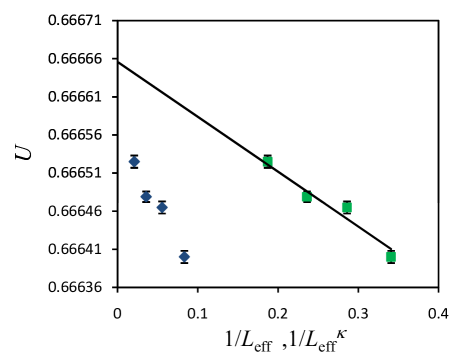
Figure 2: Binder cumulant for monopole-suppressed simulations with various lattice sizes plotted against two different abscissas. Points on left are vs. $1/L_{\mathrm{eff}}$.

For the O(4) order parameter (Coulomb Magnetization) the Binder cumulant is expected to approach 1/2 in an unmagnetized phase as the lattice size becomes infinite and 2/3 in a magnetized (spontaneously broken) phase[17]. In Fig. 2, $U$ is shown vs. $1/L_{\mathrm{eff}}$ where $L_{\mathrm{eff}}=L-12$ and $L$ is the linear lattice size which ranged from 24 to 60. $L_{\mathrm{eff}}$ is the size of the region inside the exclusion zone. One sees that $U$ is very close to 2/3 already, even for the smallest lattice size and is increasing with lattice size. This is the expected behavior in a symmetry-broken phase. To explore the extrapolation further, $U$ was assumed to behave as $1/L^{\kappa}$, where $\kappa$ is an unknown constant. A value of $\kappa=0.4$ gave the best fit. The second plot shows $U$ vs. $1/L^{k}$, showing a consistent extrapolation to $2/3$ as $L\rightarrow\infty$. Since one is within a phase here and not necessarily near a critical point, but also not deep within the phase (susceptibility is still increasing somewhat with lattice size), the expected scaling is not predicted from finite-size scaling theory. The evolution of $U$ with lattice size depends on the scaling function which is not universal, so the best one can do is a phenomenological fit. Fig. 3 shows that, also consistent with a spontaneously broken phase, the Coulomb magnetization is extrapolating to a nonzero value in the infinite lattice limit. The axes were chosen such that at a critical point one would expect a straight line through the origin. A spontaneously broken phase lies above this line and a symmetric phase lies below it.

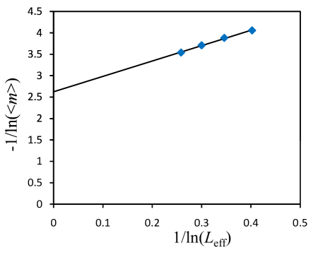
Figure 3: Coulomb magnetization for monopole-suppressed simulations with various lattice sizes.

If the remnant symmetry is broken at $\beta=0$, it almost certainly will remain broken at finite $\beta$, where the configurations are more ordered, therefore the entire $\beta$ range in the monopole-suppressed theory including the continuum limit would appear to be in a phase of broken remnant symmetry. It has been shown that such a phase is necessarily non-confining, because if the magnetization is nonzero, the lattice Coulomb potential (defined below) must approach a constant at long distances[3]. Because the lattice Coulomb potential is an upper limit to the interquark potential, the latter also is prohibited from having a linear term in the symmetry-broken phase. Supporting the above, a different method for removing violations of the non-abelian Bianchi identity also appears to remove confinement in four dimensions (but not three)[18].

Thus, it appears that eliminating SO(3) monopoles (and also Z2 strings from the plaquette constraint) eliminates confinement from the 4-d SU(2) gauge theory. However, it is important to show that the lattice spacing for this formulation is large enough for physically interesting length scales to be probed, and also so that the physical temperature associated with our largest lattice is in the region where confinement would be expected. This we will do through measurement of the lattice Coulomb potential, and from that, the running coupling.

3 Lattice Coulomb Potential

The lattice Coulomb potential, $V(R)$ is given as a function of the Coulomb magnetization equal-time two point correlation function[3],

$$aV(R)=-\mathrm{ln}(<\vec{a}(\vec{r}_{1})\cdot\vec{a}(\vec{r}_{2})>).$$ (3)

Where the two links are on the same spacelike hyperlayer with separation $R=|\vec{r}_{2}-\vec{r}_{1}|$. The expectation value is over both configurations and hyperlayers, avoiding the six closest to either boundary. It differs from the interquark potential in that the latter is derived from Wilson loops with a long time extent which allows the string connecting the quarks to attain its lowest energy state. The Coulomb potential, by contrast, creates the quark-antiquark pair with associated gluon field for an instant, so nonlinear effects of the response of the gluon vacuum are not fully included. However, as mentioned before, the Coulomb potential is an upper limit for the interquark potential, so it contains very useful information. In addition, the Coulomb potential gives a perfectly reasonable definition of the running coupling, a quantity, the behavior of which would be very interesting to know outside the perturbative region, and which within the perturbative region can also be used to determine the lattice spacing. Because it is determined from a simple link correlation function as opposed to Wilson loops large in two dimensions, the Coulomb potential can be measured to a considerably larger distance than the interquark potential, which, even when using smeared operators, is rather quickly swamped by random errors. This makes the Coulomb potential a very exciting quantity to work with, as it opens the possibility of clearly seeing the infrared behavior of the running coupling. Another considerable advantage of the Coulomb potential is that it is directly calculated - no fitting is required.

The correlation function is measured both on-axis (OA) and along body diagonal (BD) direction lines on lattices up to $60^{4}$. One can determine the effects of the finite lattice on the potential, force, and running coupling by comparing the different lattice sizes. The running coupling is defined from the potential through

$$\alpha(\sqrt{R_{1}R_{2}})=\frac{4}{3}R_{1}R_{2}(V(R_{2})-V(R_{1}))/(R_{2}-R_{1})$$ (4)

where $R_{2}$ and $R_{1}$ are distances from an initial point to adjacent lattice sites, either on-axis or along a body diagonal.

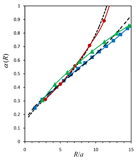
Figure 4: Running coupling in the low-R region for the $60^{4}$ lattice. Squares are OA, triangles BD. Circles are UKQCD collaboration Wilson-action data. Short-dashed line is fit to two-loop perturbative form, long-dashed line is one-loop. Error bars are smaller than plotted points.

Fig. 4 shows the running coupling for the $60^{4}$ lattice in the small-R region. Some degree of rotational non-invariance is seen between the OA and BD results, which seems to affect small-distance and large-distance results differently. More sophisticated averages of the two $R$ values used in the force determination based on the free-field lattice Fourier transform were tried, but did not reduce the rotational non-invariance, so the simpler geometric average was used, as shown above. The free field may not be a good guide to the interacting case. Also plotted is the one-parameter fit of the OA data to the two-loop renormalization group improved perturbation theory form[15]

$$\alpha(R)=\left(4\pi b_{0}\left[\ln((R_{0}/R)^{2})+(b_{1}/b_{0}^{2})\ln\ln((R_{0}/R)^{2})\right]\right)^{-1}$$ (5)

(where $b_{0}=11/24\pi^{2}$ and $b_{1}/b_{0}^{2}=102/121$) in the range $R=2a$ to $R=6a$. The OA data gives a smaller lattice spacing, so that is the more conservative choice, although averaging the lattice spacing obtained from the two datasets would probably make more sense, since they are likely extremes of the rotational non-invariance. Also shown is Wilson-action OA data of the UKQCD collaboration[19] for $\beta=2.85$, with the lattice spacing scaled for best fit at $R=5a$, which gives a factor of 0.98, the $\beta=2.85$ lattice spacing being slightly larger than that of the monopole-suppressed simulation (but the same within errors). Our $60^{4}$ lattice is therefore physically slightly larger than that of the UKQCD simulation ($48^{3}\times 56$), so there is little worry that the lattice is too small to access a region where confinement should easily be seen, if there. Also the temperature for a lattice of this size is about 1/2 of the finite-temperature deconfinement temperature, so our lattices could not be deconfined for this reason. The fit to the running coupling gives $R_{0}/a=23.5$. In this renormalization scheme $1/R_{0}$ is very close to $\Lambda_{\overline{\mathrm{MS}}}$. Since we are working with SU(2) and not the physical SU(3), it is not worth setting the scale to a high degree of precision. Taking $R_{0}^{-1}$=200 MeV, gives $a=0.043$fm with a largest lattice dimension of $60a=2.6$fm.

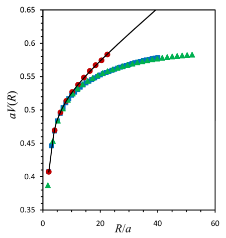
Figure 5: Coulomb potential for on-axis (squares) and body-diagonal(triangles). Also shown is UKQCD data for the interquark potential (circles). Error bars are smaller than plotted points. Fit shown to UKQCD data is linear+Coulomb.

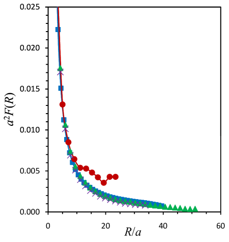
Figure 6: Coulomb force calculated through finite differences from the Coulomb potential for on-axis(squares) and body diagonal (triangles). Also shown are the $40^{4}$ BD data ($\times$), and UKQCD interquark force (circles). Errors are smaller than plotted points.

Now that the relative lattice spacings for the monopole-suppressed and Wilson-action simulations have been determined, the respective potentials (Fig. 5) and forces (Fig. 6) can be compared. For the potential a constant of 0.061 must be added to shift the UKQCD results to match at $R=4a$, and 0.0075 is added to the body-diagonal values for the same purpose. For potentials defined differently a different additive renormalization is expected. This has no effect on the physical forces. Although the two formulations agree in the perturbative small-R region, the monopole-suppressed theory clearly shows a more Coulombic form which contrasts strongly to the linear large-R confining potential of the $\beta=2.85$ Wilson-action data. The situation is most clear from the force graph. Whereas the UKQCD data show clear evidence of the force approaching a non-zero constant at large distances (string tension), no such trend is visible in the monopole-suppressed data, for which the force appears to be vanishing at large distances. The contrast is striking - clearly the two simulations cannot be made to agree. Differences between OA and BD and between $40^{4}$ and $60^{4}$ are present, but appear to be relatively minor.

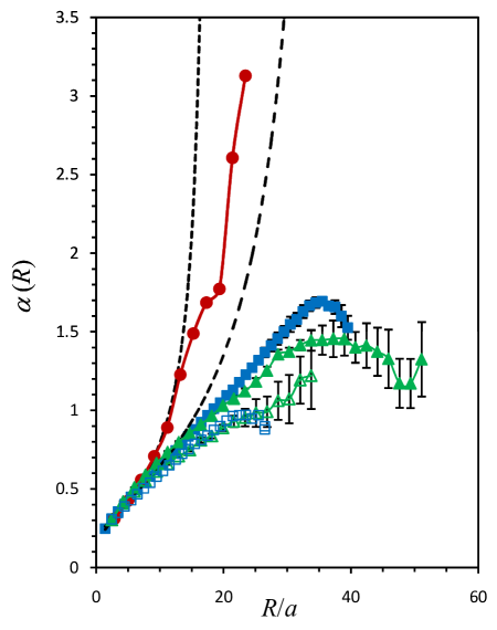
Figure 7: Running coupling for large-$R$ for $60^{4}$ OA (squares), BD (triangles) and the same for $40^{4}$ (open symbols), along with the running coupling calculated from the UKQCD interquark force (circles). Error bars are from binned fluctuations. Adjacent errors are highly correlated, so taking two-step finite differences does not reduce the error significantly. Short dash line is two-loop fit from Fig. 4 and long dashed is one-loop. The two-loop Landau pole is at $R=19a$.

Finally, the running coupling, defined above, is shown for the full lattice (Fig. 7). Here the differences between OA and BD and between $40^{4}$ and $60^{4}$ can be examined in more detail. Whereas the small-R differences between the OA and BD results are likely due to finite spacing rotational non-invariance, the large-R differences are more likely a diverging response of the different objects to finite lattice size effects. The OA and BD running couplings agree within better than 10% and follow similar trends until $R=0.5L$ for both $40^{4}$ and $60^{4}$. Because of the open boundary condition, separations beyond $R=0.5L$ can be considered since there is no second path through the boundary. However, beyond $R=0.5L$ the BD and OA no longer agree, so one can assume that the OA is feeling the finite size effect more severely here. One would expect that the BD would be reliable out to a separation $\sqrt{3}$ larger than the OA simply because there is that much more extension available along the body diagonal. This is borne out by the $40^{4}$ data which roughly follows the $60^{4}$ trend, though lies below it by 10-20%, out to $20\sqrt{3}a=35a$. This would suggest that the $60^{4}$ BD data should be reliable at this level out to $30\sqrt{3}a=52a$, which is as far as points are plotted in the figure. Up until $R=20a$ $\alpha(R)$ shows a roughly linear trend, but is slightly concave downward (as also is the one and two-loop result initially). Beyond $R=20a$ the OA potential straightens, whereas the BD continues concave downward, flattening beyond $R=35$. This is highly suggestive of an infrared fixed point. However, one cannot be absolutely sure that the BD potential is reliable beyond the place where it leaves the OA potential $R=30a$, so we are reluctant to claim an infrared fixed point without also seeing the signal in an OA potential. This, unfortunately, would require a lattice of $72^{4}$ or larger, which is beyond our present capacity. Simulations on an asymmetric $60^{3}\times 75$ lattice are currently being run in an attempt to access the OA potential out to $R=37a$. One additional point in favor of an infrared fixed point is that if one determines the second derivative of $\alpha$ in the region $R<10a$ where it can be reliably determined due to small random errors here, and extrapolate where the slope would vanish if this trend continued, that also yields a point of maximum $\alpha$ around $R=40a$. It is worth noting that $\alpha(R)$ does not necessarily have to have a fixed point in order to obtain a non-confining potential. Indeed it can actually still diverge by any power less than unity, and the potential will still be non-confining (become constant at $R\rightarrow\infty$). Thus the behavior seen here for $\alpha$ which either shows an infrared fixed point, or possibly still diverging with a slightly under linear (concave-down) behavior is fully consistent with a non-confining potential.

4 Interquark Potential

In the last section, we were comparing two somewhat different potentials, the interquark potential for the Wilson-action data and the Coulomb potential as defined in the minimal Coulomb gauge, which is expected to be an upper limit for the interquark potential. About one PC-year of computing time was devoted to the above study. At least two PC-years were devoted to determining the interquark potential using a more standard smeared operator method[19, 20]. The latter simulations were done on a $40^{4}$ lattice with ordinary periodic boundary conditions and no gauge fixing. A total of 200,000 sweeps were performed, with 5000 discarded for equilibration and loops measured every 50 sweeps. Smeared Wilson loops to size 19x19 were measured. Three different smearing levels (5, 10 and 20 iterations) were generated using the recursive blocking scheme which replaces links with a combination of the original link and U-bends. A straight-link weight of $c=2$ as defined in [19] was used. Wilson loops with both like and unlike operators at the ends were measured resulting in six different types of loops. As usual, timelike links were not smeared in order to retain the transfer-matrix interpretation. Some larger smearing levels were tried, but an indication that the simulations were possibly becoming sensitive to the lattice size through the smearing operation led us to cut the number of smearings so that information on the finite lattice size would not be fed to the observables. For each $R$, the $6\times 18$ ($T=1$ excluded) smeared Wilson loops, $W_{ik}(R,T)$ were fit to a triple exponential form

$$\sum_{j=1}^{3}p_{ij}p_{kj}\exp(-V_{j}(R)T)$$ (6)

where $p_{ij}$ are overlap coefficients between the given smeared operator ($i=1$..3) and the energy eigenstate ($j=1$..3). Since no secular trend was obvious in the excited state energies $V_{2}$ and $V_{3}$ as $R$ was varied, fits were then redone using fixed average values for the excited state energies of 0.72 and 1.33 in lattice units. This resulted in lower errors on $V(R)=V_{1}(R)$ while still giving reasonable $\chi^{2}$/d.f. values averaging 1.7. Errors in the smeared loops themselves were determined from binned fluctuations. We only studied the interquark potential on axis, because it was clear that our statistics would not allow measurement much beyond $R=18a$ which was already quite challenging.

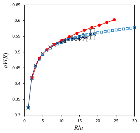
Figure 8: Interquark potential from smeared loops ($\times$) together with the Coulomb potential from Coulomb magnetization described above (squares) and UKQCD interquark potential (circles), scaled for slight difference in lattice spacing.

In Fig. 8 the interquark potential and the OA Coulomb potential are shown together, along with the UKQCD potential. These are all adjusted with an additive renormalization constant to agree at $R=4a$. The Coulomb and interquark potentials for the monopole-suppressed case appear to agree. The idea that the Coulomb potential is an upper limit of the interquark potential is really only a statement on long distance behavior, because the two differ by a finite additive normalization which is not necessarily larger for the Coulomb case. The monopole-suppressed interquark potential also appears to fall below the UKQCD result, agreeing with the trend seen earlier with the Coulomb potential which is determined to a much higher precision and as a result, to a longer distance. Agreement between the interquark and Coulomb potentials suggests that the quark color field produced by the link operators in the Coulomb gauge-fixed configuration may be quite close to the physical fields. This supports the observations of Ref. [21] where it was shown that a superposition of single-quark Coulomb fields gives a more accurate depiction of the ground state color fields of the two-quark system than a narrow flux tube does. This may mean that the effects of nonlinearity in the SU(2) color field are not actually that large.

Use of open boundary conditions with Coulomb gauge fixing is a new technology, so it is important to see that more standard methods using periodic boundary conditions and without any gauge fixing yield similar results. The precision of the Coulomb potential defined in the Coulomb gauge makes the extra effort of gauge fixing more than worthwhile. Because the force is taken from the change in potential from one $R$ to the next, which is very small, the potential must be measured to a very high accuracy in order to measure $\alpha(R)$. At $R=12$ the interquark potential simulation has an error of 0.9%. The more heavily smeared UKQCD simulation which had similar statistics achieved a random error of 0.16%. The corresponding error in the Coulomb potential is only 0.06%, with about $1/6$ the effort. Plus there is no (systematic) uncertainty from the fitting procedure. Of course one needs to remember that these are different quantities, but for this system they appear to very similar, and both can be used to obtain the running coupling. The error in potential is approximately linear in $R$. With force going like $1/R^{2}$ at the larger $R$’s its relative error grows as $R^{3}$. With the current statistics (a four month PC run) the random error on the force (and alpha) is 5% at $R=34a$. With supercomputing, combined with better tuning of the algorithms, one could imagine measuring Coulomb potentials out to distances of 80-100 lattice spacings using these techniques.

5 Conclusion

In this paper SO(3)-Z2 monopoles, which result from a topologically nontrivial realization of the non-abelian Bianchi identity are completely suppressed, along with Z2 strings and monopoles. Simulations were performed at $\beta=0$, the strong coupling limit, so the action consisted entirely of these two constraints. Since all plaquettes are in the neighborhood of the identity in the continuum limit, these constraints should not affect it. This action, in the strong coupling limit, gives a short-distance potential similar to the Wilson action at $\beta=2.85$. A fit to the two-loop running coupling allows one to find the physical lattice spacing, showing that the largest ($60^{4}$) lattice is (2.6fm)⁴. The interior region of this open boundary condition lattice where measurements were made ($48^{4}$) is (2.1fm)⁴. Here we are using physical scales that strictly apply only to SU(3) also to the SU(2) case as is usual. These lattices therefore probe the region of interest for quarkonium states, where Wilson-action simulations see a linear+Coulomb potential. The potential seen with the monopole suppressed action is much more Coulombic, and can entirely be fit with a Coulomb potential with a moderately running potential, one which is flattening out at the largest distances measured, possibly indicating an infrared fixed point of around $\alpha=1.4$. There is no evidence for a linear term which is entirely consistent with the observation of spontaneous breaking of the Coulomb-gauge remnant symmetry. Such symmetry breaking precludes the existence of linear confinement. Making $\beta$ larger will only order the configurations more, so there is almost no chance this ordered symmetry breaking would not continue to hold for $\beta>0$, including the continuum limit, $\beta\rightarrow\infty$. These results show a clear lack of universality with the Wilson action. Since all that has been done is to remove strong-coupling artifacts, the conclusion one is led to is that the confinement seen with the Wilson action is due to these strong-coupling artifacts, similar to the U(1) case, and a deconfining phase transition exists in the zero-temperature Wilson action case. This is contrary to the usual lore, but such a phase transition has be seen in the Coulomb-gauge magnetization at $\beta_{c}=3.18(8)$[1], which is consistent with the SO(3)-Z2 monopole percolation transition at $\beta=3.19(3)$ [2].

In the intermediate distance region of $R=5a$ to $R=28a$ (0.2-1.2fm), the running coupling increases roughly linearly, which means that the Coulomb force here is more like $1/R$ than $1/R^{2}$. If one integrates to get an effective potential for this region one obtains a logarithmic potential. Interestingly, phenomenological fits to quarkonium with logarithmic potentials[22] or very small powers of $R$[23] work rather well. One may not need a linear term in the potential to explain these systems. When light quarks are added to the theory, absolute confinement is destroyed anyway, so that may not be a necessary ingredient of a successful theory of the strong interactions. Sparking of the vacuum[24] and/or rearrangement of the chiral condensate[25, 26] may itself prevent color non-singlet states from existing.

6 Acknowledgement

Phillip Arndt helped with some of the computations for this paper.

References

- [1] M. Grady, arXiv:1104:3331[hep-lat].
- [2] M. Grady, Mod. Phys. Lett. A, 28 (2013) 1350087.
- [3] J. Greensite, S. Olejník, and D. Zwanziger, Phys. Rev. D 69 (2004) 074506; D. Zwanziger, Phys. Rev. Lett. 90 (2003) 102001.
- [4] E. Marinari, M. Paciello, G. Parisi, and B. Taglienti, Phys. Lett. B 298 (1993) 400 .
- [5] T.A. Degrand and D. Toussaint, Phys. Rev. D 22 (1980) 2478 .
- [6] V.G. Bornyakov, V.K. Mitrjushkin, and M. Muller-Preussker, Nucl. Phys. B (Proc. Suppl.) 30 (1995) 587.
- [7] M. Grady, arXiv:hep-lat/9806024.
- [8] J. Greensite and S. Olejník, Phys. Rev. D 67 (2003) 094503.
- [9] G. Mack and E. Pietarinen, Nucl. Phys. B205 [FS5] (1982) 141.
- [10] J. Fingberg, U.M. Heller, and V. Mitrjushkin, Nucl. Phys. B 435 (1995) 311.
- [11] G. Bhanot and M. Creutz, Phys. Rev. D 24 (1981) 3212.
- [12] G. G. Batrouni, Nucl. Phys. B 208 (1982) 467.
- [13] P. Skala, M. Faber, and M. Zach, Nucl. Phys. B 494 (1997) 293.
- [14] T.L. Ivanenko et. al., Phys. Lett. B 252 (1990) 631; T.L. Ivanenko, A.V. Pochinsky, and M.I. Polikarpov, Phys. Lett B 302 (1993) 458 ; T.G. Kovács and E.T. Tomboulis, Phys. Rev. D 57 (1998) 4054; G. Mack and V. B. Petkova, Ann. Phys. (NY) 125 (1980) 117.
- [15] M. Creutz, Phys. Rev. D 23 (1981) 1815.
- [16] M. Lüscher and S. Schaefer, arXiv:1105.4749[hep-lat].
- [17] C. Holm and W. Janke, Phys. Rev. B 48 (1993) 936.
- [18] F.V. Gubarev and S.M. Morozov, Phys. Rev. D 71 (2005) 114514.
- [19] S.P. Booth et. al., Nucl. Phys. B 394 (1993) 509.
- [20] M. Albanese et. al., Phys. Lett. B 192 (1987) 163.
- [21] T. Heinzl et. al., Phys Rev. D 78 (2008) 034504.
- [22] C. Quigg and J.L. Rosner, Phys. Lett. 71B (1977) 153.
- [23] A. Martin, Phys. Lett. B 93 (1993) 587.
- [24] V.N. Gribov, Phys. Scr. T15 (1987) 164, Phys. Lett. B 194 (1987) 119; J. Nyiri, ed., The Gribov Theory of Quark Confinement, World Scientific, Singapore, 2001.
- [25] M. Grady, Z. Phys C 39 (1988) 125; Nuovo Cim. 105A (1992) 1065; Nucl. Phys. B 713 (2005) 204.
- [26] K. Cahill and G. Herling, Nucl. Phys. B Proc. Suppl. 73 (1999) 886; K. Cahill, arXiv:hep-ph/9901285.