Exact Support Recovery
for Sparse Spikes Deconvolution
Abstract
This paper studies sparse spikes deconvolution over the space of measures. We focus on the recovery properties of the support of the measure (i.e. the location of the Dirac masses) using total variation of measures (TV) regularization. This regularization is the natural extension of the norm of vectors to the setting of measures. We show that support identification is governed by a specific solution of the dual problem (a so-called dual certificate) having minimum norm. Our main result shows that if this certificate is non-degenerate (see the definition below), when the signal-to-noise ratio is large enough TV regularization recovers the exact same number of Diracs. We show that both the locations and the amplitudes of these Diracs converge toward those of the input measure when the noise drops to zero. Moreover the non-degeneracy of this certificate can be checked by computing a so-called vanishing derivative pre-certificate. This proxy can be computed in closed form by solving a linear system. Lastly, we draw connections between the support of the recovered measure on a continuous domain and on a discretized grid. We show that when the signal-to-noise level is large enough, and provided the aforementioned dual certificate is non-degenerate, the solution of the discretized problem is supported on pairs of Diracs which are neighbors of the Diracs of the input measure. This gives a precise description of the convergence of the solution of the discretized problem toward the solution of the continuous grid-free problem, as the grid size tends to zero.
1 Introduction
1.1 Sparse Spikes Deconvolution
Super-resolution is a central problem in imaging science, and loosely speaking corresponds to recovering fine scale details from a possibly noisy input signal or image. This thus encompasses the problems of data interpolation (recovering missing sampling values on a regular grid) and deconvolution (removing acquisition blur). We refer to the review articles [27, 24] and the references therein for an overview of these problems.
We consider in our article an idealized super-resolution problem, known as sparse spikes deconvolution. It corresponds to recovering 1-D spikes (i.e. both their positions and amplitudes) from blurry and noisy measurements. These measurements are obtained by a convolution of the spikes train against a known kernel. This setup can be seen as an approximation of several imaging devices. A method of choice to perform this recovery is to introduce a sparsity-enforcing prior, among which the most popular is a -type norm, which favors the emergence of spikes in the solution.
1.2 Previous Works
Discrete regularization.
-type techniques were initially proposed in geophysics [10, 28, 23] to recover the location of density changes in the underground for seismic exploration. They were later studied in depth by David Donoho and co-workers, see for instance [14]. Their popularity in signal processing and statistics can be traced back to the development of the basis pursuit method [9] for approximation in redundant dictionaries and the Lasso method [31] for statistical estimation.
The theoretical analysis of the -regularized deconvolution was initiated by Donoho [14]. Assessing the performance of discrete regularization methods is challenging and requires to take into account both the specific properties of the operator to invert and of the signal that is aimed at being recovered. A popular approach is to assess the recovery of the positions of the non-zero coefficients. This requires to impose a well-conditioning constraint that depends on the signal of interest, as initially introduced by Fuchs [20], and studied in the statistics community under the name of “irrepresentability condition”, see [34]. A similar approach is used by Dossal and Mallat in [15] to study the problem of support stability over a discrete grid.
Imposing the exact recovery of the support of the signal to recover might be a too strong assumption. The inverse problem community rather focuses on the recovery error, which typically leads to a linear convergence rate with respect to the noise amplitude. The seminal paper of Grasmair et al. [21] gives a necessary and sufficient condition for such a convergence, which corresponds to the existence of a non-saturating dual certificate (see Section 2 for a precise definition of certificates). This can be understood as an abstract condition, which is often difficult to check on practical problems such as deconvolution.
Note that the continuous setting adopted in the present paper might be seen as a limit of such discrete problems, and in Section 5, we relate our results to well-known results on discrete grids.
Inverse problems regularization with measures.
Working over a discrete grid makes the mathematical analysis difficult. Following recent proposals [12, 4, 8, 2], we consider here this sparse deconvolution over a continuous domain, i.e. in a grid-free setting. This shift from the traditional discrete domain to a continuous one offers considerable advantages in term of mathematical analysis, allowing for the first time the emergence of almost sharp signal-dependent criteria for stable spikes recovery (see references below). Note that while the corresponding continuous recovery problem is infinite dimensional in nature, it is possible to find its solution using either provably convergent algorithms [4] or root finding methods for ideal low pass filters [8].
Inverse problem regularization over the space of measures is now well understood (see for instance [29, 4]), and requires to perform variational analysis over a non-reflexive Banach space (as in [22]), which leads to some mathematical technicalities. We capitalize on these earlier works to build our analysis of the recovery performance.
Theoretical analysis of deconvolution over the space of measures.
For deconvolution from ideal low-pass measurements, the ground-breaking paper [8] shows that it is indeed possible to construct a dual certificate by solving a linear system when the input Diracs are well-separated. This work is further refined in [7] that studies the robustness to noise. In a series of paper [2, 30] the authors study the prediction (i.e. denoising) error using the same dual certificate, but they do not consider the reconstruction error (recovery of the spikes). In our work, we use a different certificate to assess the exact recovery of the spikes when the noise is small enough.
In view of the applications of superresolution, it is crucial to understand the precise location of the recovered Diracs locations when the measurements are noisy. Partial answers to this questions are given in [19] and [1], where it is shown (under different conditions on the signal-to-noise level) that the recovered spikes are clustered tightly around the initial measure’s Diracs. In this article, we fully answer the question of the position of the recovered Diracs in the setting where the signal-to-noise ratio is large enough.
1.3 Formulation of the Problem and Contributions.
Let be a discrete measure defined on the torus , where and . We assume we are given some low-pass filtered observation . Here denotes a convolution operator with some kernel . The observation might be noisy, in which case we are given , with , instead of .
Following [8, 12], we hope to recover by solving the problem
| () |
among all Radon measures, where refers to the total variation (defined below) of . Note that in our setting, the total variation is the natural extension of the norm of finite dimensional vectors to the setting of Radon measures, and it should not be mistaken for the total variation of functions, which is routinely used to recover signals or images.
We may also consider reconstructing by solving the following penalized problem for , also known as the Beurling LASSO (see for instance [1]):
| () |
This is especially useful if the observation is noisy, in which case should be replaced with .
Four questions immediately arise:
- 1.
- 2.
- 3.
- 4.
The first question is addressed in the landmark paper [8] in the case of ideal low-pass filtering: measures whose spikes are separated enough are the unique solution of () (for data ). Several other cases (using observations different from convolutions) are also tackled in [12], particularly in the case of non-negative measures.
The second and third questions receive partial answers in [4, 7, 1, 19]. In [4] it is shown that if the solution of () is unique, the measures recovered by converge to the solution of () in the sense of the weak-* convergence when and . In [7], the authors measure the reconstruction error using the norm of a low-pass filtered version of recovered measures. In [1], error bounds are derived from the amplitudes of the reconstructed measure. In [19], bounds are given in terms of the original measure. However, those works provide little information about the structure of the measures recovered by : are they made of less spikes than or, in the contrary, do they present lots of parasitic spikes? What happens if one compels the spikes to belong to a finite grid?
The fourth question is of primary importance since most numerical schemes for sparse regularization solve a finite dimensional optimization problem over a fixed discretization grid. Following [8], one can remark that in the noiseless setting, if is recovered over the continuous domain and if its support is included in the grid, is also guaranteed to be recovered by the discretized problem. But this is of little interest in practice because the noise is likely to impact in a different manner the discrete problem and the input measure might fall outside the grid locations. Dossal and Mallat in [15] study the stability of the position of the Diracs on the grid, which leads to overly pessimistic conclusions because noise typically forces the spikes to translate over the domain. Studying the convergence of the discretized problem toward the continuous one is thus important to obtain a precise description of the discretized solution. To the best of our knowledge, the work of [2] is the only one to provide some conclusion about this convergence in term of denoising error. No previous work has studied the capability of the discretized problem to estimate in a precise manner the location of the spikes of the input measure.
Contributions.
The present paper studies in detail the structure of the recovered measure. For this purpose, we define the minimal -norm certificate. This certificate fully governs the behavior of the regularization when both and are small.
Our first contribution is a set of results indicating that the regions of saturation of the certificate (when it reaches or ) are approximately stable when and are small enough. This means that the recovered measures are supported closely to the support of the input measure if the latter is identifiable (solution of the noiseless problem ()).
Our second contribution introduces the Non Degenerate Source Condition, which imposes that the second derivative of the minimal-norm certificate does not vanish on the saturation points. Under this condition, we show that for and small enough, the reconstructed measure has exactly the same number of spikes as the original measure and that their locations and amplitudes converge to those of the original one.
Our third contribution shows that under the Non Degenerate Source Condition, the minimal norm certificate can actually be computed in closed form by simply solving a linear system. This in turn also implies that the errors in the amplitudes and locations decay linearly with respect to the noise level.
Our fourth and last contribution focuses on the regularization over a discrete finite grid, which corresponds to the so-called Lasso or Basis Pursuit Denoising problem. We show that when and are small enough, and provided that the Non Degenerate Source Condition holds, the discretized solution is located on pairs of Diracs adjacent to the input Diracs location. This gives a precise description of how the solution to the discretized problem converges to the one of the continuous problem when the stepsize of the grid vanishes.
Throughout the paper, the proposed definitions and results are illustrated in the case of the ideal low-pass filter, showing that the assumptions are actually relevant. Note that the code to reproduce the figures of this article is available online111https://github.com/gpeyre/2013-FOCM-SparseSpikes/.
Outline of the paper.
Section 2 defines the framework for the recovery of Radon measures using total variation minimization. We also expose basic results that are used throughout the paper. Section 3 is devoted to the main result of the paper: we define the Non Degenerate Source Condition and we show that it implies the robustness of the reconstruction using . In Section 4 we show how the specific dual certificate involved in the Non Degenerate Source Condition can be computed numerically by solving a linear system. Lastly, Section 5 focuses on the recovery of measures on a discrete grid.
1.4 Notations
For any Radon measure defined on , we denote its support by . If is a finite set (in which case we say that is a discrete measure) and , then is of the form , where , , and and for all . In the rest of the paper, we shall write to hint that has the above decomposition (implying that and for all ).
We also define the signed support:
where (resp. ) denotes the positive (resp. negative) part of . For a discrete measure ,
We shall consider restrictions of measures and functions to subsets of . For a discrete measure and a finite set, we define
For a continuous function defined on , we define
Given a convolution operator with kernel , we define (resp. , ) by
| (1) | ||||
| (2) | ||||
| (3) |
We define
| (4) | ||||
| (5) |
Eventually, in order to study small noise regimes, we shall consider domains , for , , where:
| (6) |
2 Preliminaries
In this section, we precise the framework and we state the basic results needed in the next sections. We refer to [5] for aspects regarding functional analysis and to [17] as far as duality in optimization is concerned.
2.1 Topology of Radon Measures
Since is compact, the space of Radon measures can be defined as the dual of the space of continuous functions on , endowed with the uniform norm. It is naturally a Banach space when endowed with the dual norm (also known as the total variation), defined as
| (7) |
In that case, the dual of is a complicated space, and it is strictly larger than as is not reflexive.
However, if we endow with its weak-* topology (i.e. the coarsest topology such that the elements of define continuous linear forms on ), then is a locally convex space whose dual is .
In the following, we endow (respectively ) with its weak (respectively its weak-*) topology so that both have symmetrical roles: one is the dual of the other, and conversely. Moreover, since is separable, the set endowed with the weak-* topology is metrizable.
Given a function , we define an operator as
It can be shown using Fubini’s theorem that is weak-* to weak continuous. Moreover, its adjoint operator is defined as
2.2 Subdifferential of the Total Variation
It is clear from the definition of the total variation in (7) that it is convex lower semi-continuous with respect to the weak-* topology. Its subdifferential is defined as
| (8) |
for any such that .
Since the total variation is a sublinear function, its subgradient has a special structure. One may show (see Proposition 12 in Appendix A) that
| (9) |
In particular, when is a measure with finite support, i.e. for some , with and distinct
| (10) |
2.3 Primal and Dual Problems
Given an observation for some , we consider reconstructing by solving either the relaxed problem for
| () |
or the constrained problem
| () |
If is the unique solution of (), we say that is identifiable.
In the case where the observation is noisy (i.e. the observation is replaced with for ), we attempt to reconstruct by solving for a well-chosen value of .
Existence of solutions for () is shown in [4], and existence of solutions for () can be checked using the direct method of the calculus of variations (recall that for (), we assume that the observation is ).
A straightforward approach to studying the solutions of Problem () is then to apply Fermat’s rule: a discrete measure is a solution of if and only if there exists such that
with and for .
Another source of information for the study of Problems () and () is given by their associated dual problems. In the case of the ideal low-pass filter, this approach is also the key to the numerical algorithms used in [2, 8, 1]: the dual problem can be recast into a finite-dimensional problem.
The Fenchel dual problem to () is given by
| () |
which may be reformulated as a projection on a closed convex set (see [4, 1])
| () |
This formulation immediately yields existence and uniqueness of a solution to ().
The dual problem to () is given by
| () |
Contrary to (), the existence of a solution to () is not always guaranteed, so that in the following (see Definition 5) we make this assumption.
2.4 Dual Certificates
The strong duality between and () is proved in [4, Prop. 2] by seeing () as a predual problem for (). As a consequence, both problems have the same value and any solution of () is linked with the unique solution of () by the extremality condition
| (13) |
Moreover, given a pair , if relations (13) hold, then is a solution to Problem () and is the unique solution to Problem ().
As for (), a proof of strong duality is given in Appendix A (see Proposition 13). If a solution to () exists, then it is linked to any solution of () by
| (14) |
and similarly, given a pair , if relation (14) hold, then is a solution to Problem () and is a solution to Problem ()).
Since finding which satisfies (14) gives a quick proof that is a solution of (), we call a dual certificate for . We may also use a similar terminology for and Problem ().
In general, dual certificates for () are not unique, but we consider in the following definition a specific one, which is crucial for our analysis.
Definition 1 (Minimal-norm certificate).
Observe that in the above definition, is well-defined provided there exists a solution to Problem (), since is then the projection of onto the non-empty closed convex set of solutions. Moreover, in view of the extremality conditions (14), given any solution to (), it may be expressed as
| (16) |
Proposition 1 (Convergence of dual certificates).
Let be the unique solution of Problem (), and be the solution of Problem () with minimal norm defined in (15). Then
Moreover the dual certificates for Problem () converge to the minimal norm certificate . More precisely,
| (17) |
in the sense of the uniform convergence.
Proof.
Let be the unique solution of (). By optimality of (resp. ) for () (resp. ())
| (18) | ||||
| (19) |
As a consequence for all .
Now, let be any sequence of positive parameters converging to . The sequence being bounded in , we may extract a subsequence (denoted ) such that weakly converges to some . Passing to the limit in (18), we get . Moreover, weakly converges to in , so that , and is therefore a solution of ().
But one has
hence and in fact . As a consequence, converges to for the strong topology as well. This being true any sequence , we get the result claimed for : assume by contradiction that there exists and a sequence such that for all . By the above argument we may extract a subsequence which converges towards , which contradicts . Hence strongly in .
It remains to prove the convergence of the dual certificates. Observing that , we get
where does not depend on nor , hence the uniform convergence. ∎
2.5 Application to the ideal Low-pass filter
In this paragraph, we apply the above duality results to the particular case of the Dirichlet kernel, defined as
| (20) |
It is well known that in this case the spaces and are finite-dimensional, being the space of real trigonometric polynomials with degree less than or equal to .
We first check that a solution to () always exists. As a consequence, given any measure , the minimal norm certificate is well defined.
Proposition 2 (Existence of ).
Proof.
A striking result of [8] is that discrete measures are identifiable provided that their support is separated enough, i.e. for some , where is the so-called minimum separation distance.
Definition 2 (Minimum separation).
The minimum separation of the support of a discrete measure is defined as
where is the distance on the torus between and , and we assume .
In [8] it is proved that for complex measures (i.e. of the form for and ) and for real measures (i.e. of the form for and ). Extrapolating from numerical simulations on a finite grid, the authors conjecture that for complex measures, one has . In this section we apply results from Section 2.4 to show that for real measures, necessarily .
We rely on the following theorem, proved by P. Turán [32].
Theorem 1 (Turán).
Let be a non trivial polynomial of degree such that . Then for any root of on the unit circle, . Moreover, if , then for some .
Corollary 1 (Non identifiable measures).
Proof.
Let , assume by contradiction that is a solution of (), and let be an associated dual certificate (which exists since is finite-dimensional). Then necessarily and and by the intermediate value theorem, there exists such that .
Writing , the polynomial satisfies , and .
By Theorem 1, we cannot have nor , hence and , so that . But this implies , which contradicts the optimality of . ∎
In a similar way, we may also deduce the following corollary.
Corollary 2 (Opposite spikes separation).
Let be any discrete measure solution of Problem or where for any data and any noise . If there exists (resp. ) such that (resp. ), then .
3 Noise Robustness
This section is devoted to the study of the behavior of solutions to for small values of and . In order to study such regimes, as already defined in (6), we consider sets of the form
for and .
First, we introduce the notion of extended support of a measure. Then we show that this concept governs the structure of solutions at small noise regime. After introducing the Non Degenerate Source Condition, we state the main result of the paper, i.e. that under this assumption, the solutions of have the same number of spikes as the original measure, and that these spikes converge smoothly to those of the original measure.
3.1 Extended signed support
Our first step in understanding the behavior of solutions to at low noise regime is to introduce the notion of extended signed support.
Definition 3 (Extended signed support).
Let such that there exists a solution to () (where as usual ), and let be the associated minimal norm certificate.
The extended support of is defined as:
| (21) |
and the extended signed support of as:
| (22) |
Notice that and actually depend on rather than on itself. For any measure , the (signed) support and the extended (signed) support of are in general not related. Yet, from the optimality conditions (14) we observe:
Proposition 3.
3.2 Local behavior of the support
In this paragraph, we focus on the local properties of the support of solutions to at low noise regime. As usual, we denote for some . For now, we make as few assumptions as possible on . In particular, we do not assume that has full rank. Any solution to (which is not necessarily unique) is denoted by .
Lemma 1.
In particular, if consists in isolated points , Lemma 1 states that all the mass of is concentrated in boxes , where when . Moreover, in each box, has the sign of .
Also, if (i.e. ), we see that for and small enough (in fact, any and suffices, as can be seen from (13)).
Proof.
We split the proof in several parts.
Behavior of the minimal norm certificate.
Let us consider the sets:
From the uniform continuity of , for small enough, in and in , so that .
If , the set being compact, . We define .
If , the connectedness of implies that and , or conversely. In that case we define .
In any case, we see that for all , if , then
| (24) |
Variations of dual certificates.
Let be the solution of the noiseless problem () and be the solution of the noisy dual problem for . Since the mapping is a projection onto a convex set (see ()), it is non-expansive, i.e.
| (25) |
As a consequence, if (resp. ) is the dual certificate of the noiseless (resp. noisy) problem, we have
| (26) |
for some (in fact ).
Structure of the reconstructed measure.
By (24) for and using the extremality conditions we obtain that and that (resp. ) is non-negative in (resp. ). Indeed, the extremality conditions impose that , -almost everywhere, hence the claimed result. ∎
Lemma 1 does not make any assumption on the local structure of , and does not provide any information on the local structure of either (it might even not be discrete). If we assume that for some , then the reconstructed measure has at most one spike in the neighborhood of .
Lemma 2.
Proof.
The proof follows the same steps as those of Lemma 1.
Behavior of the minimal norm certificate.
First, observe that if and (resp. ) for , then (resp. ). As a consequence, is an isolated point of . For small enough, and for all .
Variations of dual certificates.
We set with and we impose , so that
thus for small enough.
Structure of the reconstructed measure.
From the above inequality, we know that is strictly concave (resp. strictly convex) in . As a result, there is at most one point in such that (resp. ).
If is identifiable, it remains to prove that there is indeed one spike in . This is obtained by relying on a result by Bredies and Pikkarainen [4] which is an application of [22, Th. 3.5]. It guarantees that converges to for the weak-* topology when . We recall the result below (see Proposition 4) for the convenience of the reader.
By weak-* convergence of to for and , must converge to . By the optimality conditions, we see that , so that and , hence the result. ∎
In the proof of Lemma 2 we have relied on the following result.
3.3 Non Degenerate Source Condition
The notion of extended signed support has strong connections with the source condition introduced in [6] to derive convergence rates for the Bregman distance.
Definition 4 (Source Condition).
A measure satisfies the source condition if there exists such that
In a finite-dimensional framework, the source condition is simply equivalent to the optimality of for () given . In the framework of Radon measures, the source condition amounts to assuming that is a solution of () and that there exists a solution to (). In fact, the source condition simply means that the conditions of Proposition 3 hold.
If one is interested in being the unique solution of () for (in which case we say that is identifiable), the source condition may be strengthened to give a sufficient condition.
Proposition 5 ([12, Lemma 1.1]).
In this paper, in view of Lemma 2, we strengthen a bit more the Source Condition so as to derive a global stability result concerning the support of the solutions of (see Theorem 2).
Definition 5 (Non Degenerate Source Condition).
Let be a discrete measure, and . We say that satisfies the Non Degenerate Source Condition (NDSC) if
-
•
there exists such that .
-
•
the minimal norm certificate satisfies
In that case, we say that is not degenerate.
The first assumption in the above definition is the standard Source Condition. The last two assumptions impose conditions on the extended signed support, namely that and for all .
When is an ideal low-pass filter with cutoff frequency , there are numerical evidences that measures having a large enough separation distance (proportional to ) satisfy the non degenerate source condition, see Section 4.
3.4 Main Result
The following theorem, which is the main result of this paper, gives a global result on the precise structure of the solution when the signal-to-noise ratio is large enough and is small enough.
Theorem 2 (Noise robustness).
Let be a discrete measure. Assume that (defined in (4)) has full rank and that satisfies the Non Degenerate Source Condition.
Then there exists , such that for , the solution of is unique and is composed of exactly spikes.
Moreover, up to a permutation of indices, we may write with and (for ), and writing , the mapping
is whenever ().
In particular, for , we have
| (28) |
Proof.
Applying Lemma 2 at each point for and Lemma 1, we see that for small enough, there exists , such that has at most one spike in each interval , and
In fact, since has full rank, has full rank as well and is identifiable (by Proposition 3). Therefore, Lemma 2 ensures that there is indeed one spike in each interval, with sign equal to .
It remains to prove the uniqueness of the amplitudes and locations and their smoothness as function of . To this end, we observe that they satisfy the following implicit equation
where , and
Indeed, this implicit equation simply states that , and that .
Since is a function defined on , we may apply the implicit functions theorem.
The derivative of with respect to and reads
so that for , and using , one obtains
Since we assume has full rank, then is invertible and the implicit functions theorem applies: there is a neighborhood of in and a function such that
Moreover, writing , we have
-
•
,
-
•
for any , ,
-
•
if (for ), then .
The constructed amplitudes and locations coincide with those of the solutions of for all such that . Possibly changing the value of so that , we obtain the desired result. ∎
Remark 1.
Although this paper focuses on identifiable measures, Theorem 2 describes the evolution of the solutions of for any input measure such that there exists which satisfies the non degenerate source condition and . Instead of converging towards , the solutions will converge towards .
3.5 Extensions
Theorem 2 extends in a straightforward manner to higher dimensions, i.e. when replacing by for . In the NDSC introduced in Definition 5, one should replace, for , the constraint by the constraint that the Hessian is invertible.
The proof also extends to non-stationary filtering operators, i.e. which can be written as
where .
3.6 Application to the ideal Low-pass filter
We first observe that the injectivity condition on assumed in Theorem 2 always holds.
Proposition 6 (Injectivity of ).
Let with for and . Then has full rank.
The proof is given in Appendix B.
 |
 |
| (a) and | (b) |
 |
 |
| (c) | (d) |
As to whether or not the Non Degenerate Source Condition holds for discrete measures, we will discuss this matter in Section 4 more in depth. For now, let us mention that we have observed empirically that this condition holds under the hypotheses of Theorem in [8], namely that , but also with measures with far smaller values of .
 |
 |
| (a) and | (b) |
 |
 |
| (c) | (d) |
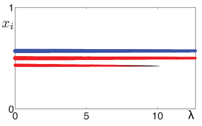
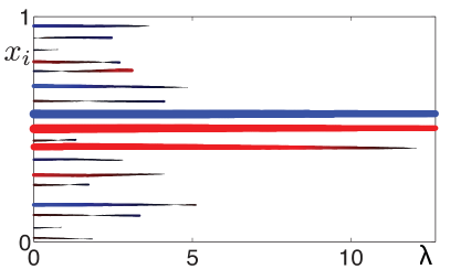
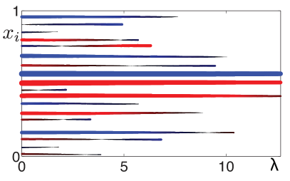
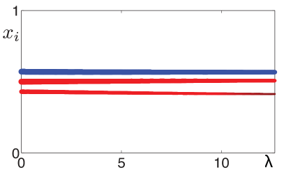
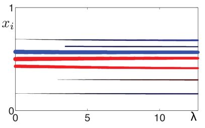
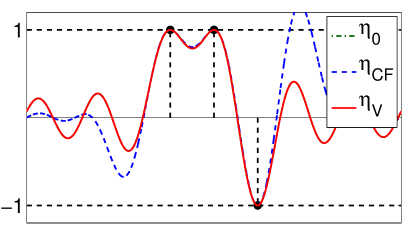
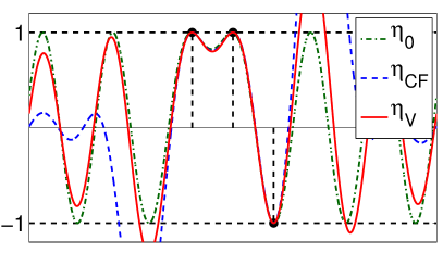
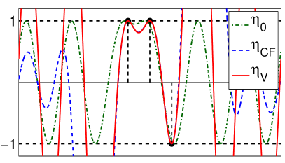
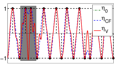
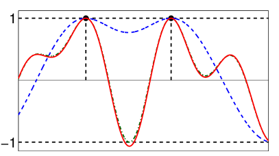
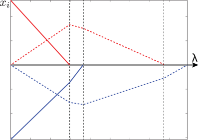
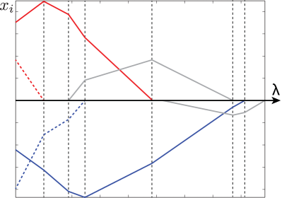
Figure 1 shows the whole solution path of the solutions of when and the input measure is identifiable and has three spikes separated by . Such a measure satisfies the Non-degenerate Source Condition as shown in plot (a). The plots (b,c,d) illustrate the conclusion of Theorem 2. For values of which are too small with respect to , the solution is perturbed with spurious spikes, but as soon as is large enough, has a support that closely (but not exactly) matches the one of . For large value of , spikes starts disappearing, and the support is not correctly estimated. Figure 2 shows the solutions of , i.e. the noise is scaled by the regularization parameter . In accordance with Theorem 2, this shows that for , the support of the spikes is precisely estimated.
4 Vanishing Derivatives Pre-certificate
We show in this section that, if the Non Degenerate Source Condition holds, the minimal norm certificate is characterized by its values on the support of and the fact that its derivative must vanish on the support of . Thus, one may compute the minimal norm certificate simply by solving a linear system, without handling the cumbersome constraint .
4.1 Dual Pre-certificates
Loosely speaking, we call pre-certificate any “good candidate” for a solution of (14). Typically, a pre-certificate is built by solving a linear system (with possibly a condition on its norm). The following pre-certificate appears naturally in our analysis.
Definition 6 (Vanishing derivative pre-certificate).
The vanishing derivative pre-certificate associated with a measure is where
| (31) |
It is clear that if the Source Condition (see Definition 4) holds, then exists (since Problem (31) is feasible). Observe that, in general, is not a certificate for since it does not satisfy the constraint . The following proposition gathers several facts about the vanishing derivative pre-certificate which show that it is indeed a good candidate for the minimal norm certificate.
Proposition 7.
Let be a discrete measure. The following assertions hold.
The third assertion of Proposition 7 states that it is equivalent to check the Non Degenerate Source Condition on (Definition 5) or to check the same conditions on . In case those conditions hold, one even has (first assertion). The main point of this equivalence is that the second assertion yields a practical expression to compute which may be used in numerical experiments (see Section 4.3).
Proof.
For the first assertion, we observe that if Problem (31) is feasible (and thus exists) and , then and the Source Condition holds. Hence, . On the other hand the minimal norm certificate must satisfy all the constraints of (31), thus the minimality of the norms of both and implies that . The converse implication is obvious.
For the second assertion, Problem (31) can be written as
which is a quadratic optimization problem in a Hilbert space with a finite number of affine equality constraints. Moreover, the assumption that has full rank implies that the constraints are qualified. Hence it can be solved by introducing Lagrange multipliers and for the constraints. One should therefore solve the following linear system to obtain the value of
Solving for in these equations gives the result.
For the third assertion, if the Non Degenerate Source condition holds, we apply Theorem 2 which yields a path of solutions of (we consider the case ). Then from Proposition 8 below, we obtain that is a valid certificate and , hence is non-degenerate. The converse implication is a straightforward consequence of the first assertion. ∎
4.2 Necessary condition for support recovery
There is a priori no reason for the vanishing derivative pre-certificate to satisfy . Here, we prove that that is in fact a necessary condition for (noiseless) exact support recovery to hold on some interval with , i.e. the solutions of having exactly spikes which converge smoothly towards those of the original measure.
Proposition 8.
Let be a discrete measure such that has full rank. Assume that there exists and a path , such that for all the measure is a solution to (the noiseless problem).
Then exists, and .
Proof.
Let be the certificate defined by the optimality conditions (13). We show that converges towards (and that the latter exists).
Writing
we observe that for any and any ,
and the latter integral converges (uniformly in ) to zero when by uniform continuity of its integrand (since , and are ). As a consequence, we obtain that converges uniformly to .
On the other hand, we observe that for small enough, , and using the notations of the proof of Theorem 2, the implicit equation holds. Differentiating that equation at we obtain:
or equivalently
As a consequence, Problem (31) is feasible and we see that converges uniformly (and thus in the strong topology) to and converges uniformly to (which is precisely from the second assertion of Proposition 7).
Since for all , we obtain that , hence the claimed result. ∎
4.3 Application to the Ideal Low-pass Filter
In order to prove their identifiability result for measures, the authors of [8] also introduce a “good candidate” for a dual certificate associated with for and . For being the square of the Fejer kernel, they build a trigonometric polynomial
and compute by imposing that and .
They show that the constructed pre-certificate is indeed a certificate, i.e. that , provided that the support is separated enough (i.e. when ). This result is important since it proves that measures that have sufficiently separated spikes are identifiable. Furthermore, using the fact that is not degenerate (i.e. for all ), the same authors derive an robustness to noise result in [7], and Fernandez-Granda and Azais et al. use the constructed certificate to analyze finely the local averages of the spikes in [19, 1].
From a numerical perspective, we have investigated how this pre-certificate compares with the vanishing derivative pre-certificate that appears naturally in our analysis, by generating real-valued measures for different separation distances and observing when each pre-certificate satisfies .
As predicted by the result of [8], we observe numerically that the pre-certificate is a certificate (i.e. ) for any measure with . We also observe that this continues to hold up to . Yet, below , it may happen that some measures are still identifiable (as asserted using the vanishing derivative pre-certificate ) but stops being a certificate, i.e. . A typical example is shown in Figure 3, where, for we have used three equally spaced masses as an input, their separation distance being . Here, we have computed an approximation of the minimal norm certificate by solving () with very small .
For , both and are certificates, so that the vanishing derivatives pre-certificate is equal to the minimal norm certificate . For , violates the constraint but the vanishing derivative pre-certificates is still a certificate (even showing that the measure is identifiable). For and , neither nor satisfy the constraint, hence . Yet, ensures that is a solution to ().
From the experiments we have carried out, we have observed that the vanishing derivative pre-certificate behaves in general at least as well as the square Fejer . The only exceptions we have noticed is for a large number of peaks (when is close to ), with . This is illustrated in Figure 4 which shows a measure for which is a non-degenerate certificate (which shows that it is identifiable), but for which since (thus is not a certificate). Typically, we have in this case . Such a measure is identifiable but there is no support recovery for (in the sense of Proposition 8), hence its support is not stable.
Such pathological cases are relatively rare. An intuitive explanation for this is the fact that having for or for some tend to impose a large norm, thus contradicting the minimality of (recall that when is an ideal low pass filter ).
5 Discrete Sparse Spikes Deconvolution
5.1 Finite Dimensional Regularization
A popular way to compute approximate solutions to () with fast algorithms is to solve this problem on a finite discrete grid . Denoting by the cardinal of the grid , and by the finite sequence of elements of , the idea is to solve (or ) with the additional constraint that for some .
This is nothing but the so-called basis pursuit denoising problem [9], also known as the Lasso [31] in statistics. Indeed, defining the linear operator through
the problem amounts to:
| () |
where is a linear operator ( may as well be replaced with or any Hilbert space), and denotes the mass at each point of the grid. In the noiseless case, the exact reconstruction problem reads:
| () |
The aim of the present section is to study the asymptotic of Problems () and () as the stepsize of the grid vanishes. To this end, we keep the framework of measures and we reformulate the constraint that , i.e. that can be written as , where . Recall that the notation hints that for all and that the ’s are all distinct, so that in general . We thus adopt the following penalization term
| (32) |
so that when , and otherwise.
5.2 Certificates over a Discrete Grid
We also introduce the corresponding dual problems:
| () |
| () |
Remark 2.
Let us denote by the image by of all measures with support in . It may happen (for instance if the grid is too rough) that , in which case () is not feasible and () has infinite value. But () is then equivalent to where is an orthogonal decomposition. Problem () is thus an approximation of , and the relevant dual problems are and . For the sake of simplicity, we shall assume from now on that , but the reader may keep in mind that this hypothesis can be withdrawn by replacing with .
In view of Remark 2, we observe that problems () and () are in fact finite dimensional. Indeed, their constraints being invariant by addition of elements of , we may consider their quotient with the space . Therefore the condition may be reduced to where is a finite dimensional space.
5.3 Noise Robustness
As in the continuous case (cf. Section 3), the support of the solutions of for and is governed by the minimal norm certificate. We introduce here the discrete counterpart of the extended support of a measure.
Definition 7 (Extended support).
Let such that , and let be the discrete minimal norm certificate defined in (34). The extended support of relatively to is defined as
| (35) |
and the extended signed support relatively to as
| (36) |
It is important to notice that the assumption does not mean that the support of is included in , but that there exists a measure with support included in which produces the same observation . Therefore the support of and its extended support may even be disjoint.
Theorem 3 (Noise robustness, discrete case).
Let such that . Then, there exists , such that for (defined in (6)) any solution of satisfies:
| (37) |
If, in addition, has full rank and is a solution of (), then the solution is unique, is identifiable and choosing ensures , where
Proof.
The proof is essentially the same as in the continuous case, therefore we only sketch it. To simplify the notation, we write . The solutions of () converge to for , where is the discrete minimal norm certificate.
By the triangle inequality
Thus, there exist two constants and , such that for and , for any . Then, the primal-dual extremality conditions imply that for any solution of , one has and equality of the signs.
Now, if has full rank, we can invert the extremality condition:
Observing that , we obtain the -robustness result. ∎
Theorem 3 is analogous to Lemma 1 for the continuous problem. The discrete nature of the problem makes its conclusions more precise. Although the -robustness results are similar to those of Theorem 2, the focus here is a bit more general, in the sense that this theorem does not assert that the support of the recovered measures matches the support of the input measure . In fact, if is a solution to (), , so that the recovered solutions to have in general more spikes than , and the spikes in must vanish as .
In order to get the exact recovery of the signed support for small noise, we may assume in addition that so as to obtain a result analogous to Theorem 2. Precisely, we obtain the following theorem which was initially proved by Fuchs [20]. First, we introduce a pre-certificate.
Definition 8 (Fuchs pre-certificate).
Let such that . We define the Fuchs pre-certificate as
| (38) |
This pre-certificate, introduced in [20], is a certificate for if and only if , in which case it is equal to the discrete minimal norm pre-certificate .
If has full rank, then can be computed by solving a linear system:
Corollary 3 (Exact support recovery, discrete case,[20]).
Let such that , and that has full rank. If for all , then is identifiable for and there exists , such that for the solution of is unique and satisfies . Moreover
| (39) |
where .
The condition for all is often called the irrepresentability condition in the statistics literature, see [34]. This condition can be shown to be almost a necessary and sufficient condition to ensure exact recovery of the support of . For instance, if for some , one can show that for all where is any solution of , see [33]. In our framework, we see that this irrepresentability condition means that the precertificate is indeed a certificate (so that it is equal to the minimal norm certificate), and that its saturation set is equal to the support of .
For deconvolution problems, an important issue is that Corollary 3 is useless when studying the stability of the original infinite dimensional problem (). Indeed, the pre-certificate (38) is not constrained to have vanishing derivatives, so that it generally takes some values strictly greater than for a generic discrete input measure . When the stepsize of the grid is small enough, such values are sampled and necessarily becomes strictly larger than one. As detailed in Section 4, when shifting from the discrete grid setting to the continuous setting, the natural pre-certificate to consider is the vanishing derivative pre-certificate defined in (31), and not the pre-certificate .
5.4 Structure of the Extended Support for Thin Grids
In the previous section, we have introduced the notion of extended signed support of a measure relatively to a grid , and we have proved that this set, , contains the signed supports of all the reconstructed measures for small noise. In this section, we focus on the structure of the extended support. We show that, if the support of belongs to the grid for a sufficiently small stepsize and if the Non Degenerate Source Condition holds, the extended signed support consists in the signed support of and possibly one immediate neighbor with the same sign for each spike. Therefore, when the grid stepsize is small enough, the support of the measure is generally not stable for the discrete problem, but the support of the reconstructed measure is a close approximation of the original one.
From now on, for the sake of simplicity, we consider dyadic grids . The constraint sets in and () are denoted respectively by
| (40) | ||||
| (41) |
The structure of for large is intimately related to the convergence of to . First, let us notice the following result, whose proof is given in Appendix C.
Proposition 9 (Convergence for fixed ).
Proposition 9 simply states that the projection onto convex sets which converge (in the sense of set convergence) to converges to the projection onto . However, the case is not as straightforward, and for instance one cannot easily swap the limits in (44). In fact, given any decreasing sequence of polyhedra , it is not true in general that the minimal norm solution of should converge to the minimal norm solution of where . As a consequence it is not clear to us whether this convergence always holds for polyhedra of the form
However, when the spikes locations belong to the grid for large enough, the convergence of the minimal norm certificates holds. In the case of dyadic grids, this is equivalent to being a discrete dyadic measure, i.e. such that for some :
| (45) |
The proofs given below make use of a remark given in [8]: if a solution of the continuous problem () has support in the grid , then it is also a solution of the discrete problem ().
Proposition 10 (Convergence for dyadic measures).
Let be a discrete dyadic measure (see (45)), and assume that the (possibly degenerate) source condition holds. Then
| (46) | ||||
| (47) |
where (resp. ) denotes the corresponding minimal norm certificate.
Proof.
First, following [8], we observe that, since and (a fortiori for ), is also a dual certificate for provided . As a consequence .
The sequence being bounded in , we may extract a subsequence (still denoted by ) which weakly converges to some , and
| (48) |
Moreover, by optimality of for the discrete problem, for each , so that in the limit . Observing that (since each is weakly closed) we conclude that . Since the limit does not depend on the extracted subsequence, we conclude that the whole sequence converges to , and equality in (48) implies that the convergence is strong.
The consequence regarding is straightforward. ∎
We may now describe the structure of the extended support for dyadic measures which satisfy the Non Degenerate Source Condition.
Proposition 11 (Extended support).
Let be a discrete dyadic measure which satisfies the Non Degenerate Source Condition. Then, for large enough, there exists such that:
| (49) |
where .
Corollary 4.
Under the hypotheses of Proposition 11, for large enough, there exist two constants and such that, for and , any solution of has support in , with signs , .
Proof of Proposition 11.
We describe the points where the value of may be . By the Non-Degenerate Source Condition, there exists small enough such that the intervals , , do not intersect, and that for all , and . Moreover, with .
Therefore, by Proposition 10, for large enough:
-
•
for ,
-
•
for ,
-
•
,
and in each interval , has the same sign as and it is strictly concave (resp. strictly convex) if (resp. ).
Assume for instance that . The extremality conditions between and for also imply that is a solution of . Then, the extremality conditions between and imply that as well. By the strict concavity of there is at most one other point such that , and since , . Such a point contributes to the extended support of if and only if it belongs to the grid (i.e. ).
The argument for is similar. This concludes the proof. ∎
Corollary 4 highlights the difference between the continuous and the discretized problems. In the first case, any small noise would induce a slight perturbation of the spikes locations and amplitudes, but their number would stay the same. In the second case, the spikes cannot “move”, so that new spikes may appear, but only at one of the immediate neighbors of the original ones.
For non-dyadic measures, we may show using Proposition 9 that for small, fixed , and large enough, there is at most one pair of spikes (located at consecutive points of the grid) in the neighborhood of each original spike. From our numerical experiments described below (in the case of the ideal low-pass filter), we conjecture that, in the case where there are indeed two spikes, they surround the location of the original spike.
5.5 Application to the Ideal Low-pass Filter
To conclude this section, we compare the different (pre-)certificates involved in the above discussion, whether on the discrete grid or in the continuous domain. Then we illustrate the convergence of the sets towards .
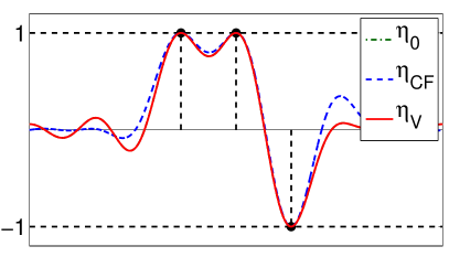
Certificates.
Figure 5 illustrates the results of Section 5.4. The numerical values are , , and the distance between the two opposite spikes is . The continuous minimal norm certificate is shown: it satisfies for all and for . The discrete minimal norm certificate satisfies for all in the grid, and for all in the neighborhood of . For a dyadic measure, such points are and possibly one of its immediate neighbors. For non dyadic measures, we conjecture that such points are the two immediate neighbors of .
The Fuchs precertificate is also shown. Some points of the grid do not satisfy , hence the Fuchs pre-certificate is not a certificate and the support is not stable. This was already clear from the fact that .
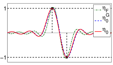
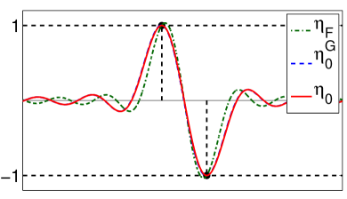
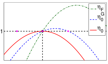
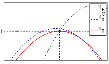
Figure 6 focuses on the reconstructed amplitudes using as . Each curve represents a path . Note that for the problem on a finite grid, such paths are piecewise affine. In the dyadic case (left part of the figure), the amplitude at (continuous line) and at the next point of the grid (dashed line) are shown. As , the spike at the neighbor vanishes and the result tends to the original identifiable measure. In the non dyadic case (right part of the figure), the amplitude at the two immediate neighbors of are shown (continuous and dashed lines). Here so that is not identifiable for the discrete problem. For each spike, the amplitudes of the two neighbors converge to some non zero value. The limit measure as is the solution of .
Set convergence.
Now, we interpret the convergence of the discrete problems through the convergence of the corresponding constraint set for the dual problem. Writing with , we observe that:
| (50) | ||||
| (51) |
As a consequence is the polar set of the convex hull of .
In the case of the Dirichlet kernel, the vector space is the space of trigonometric polynomials with degree less than or equal to . An orthonormal basis of is given by: where , and for .
Moreover,
so that we may write:
For , we obtain , and the vectors lie on a circle. The convex hull of is thus a cylinder, and its polar set is displayed in Figure 7 for , , and .
Problem corresponds to the projection of onto the polytope . Each face of corresponds to a possible signed support of the solutions . The large, flat faces of yield stability to the support of for small noise , as described by Theorem 3. As these faces converge into a piecewise smooth manifold and the support of is allowed to vary smoothly in , according to Theorem 2.
Conclusion
In this paper, we have given a precise statement about the support recovery property of sparse spikes deconvolution with total variation regularization. This support recovery is governed by the non-degeneracy of a minimal norm certificate. This hypothesis can be checked by computing a vanishing derivative pre-certificate, which can be computed in closed form. We have shown that under this non-degeneracy hypothesis, one recovers the same number of spikes and that these spikes converge to the original ones when and are small enough. While previous stability results [7, 19, 1] hold for an arbitrary noise level and make use of any non-degenerate certificate, they are formulated in terms of local averages of the recovered measure and do not describe precisely the support. In contrast, our result which requires a specific certificate to be non-degenerate and a regime where and are small enough provides exact support stability. These settings and results are thus not comparable, and provide complementary informations about the performance of total variation regularization.
Developing a similar framework for the discrete setting, we have also improved upon existing results about stability of the support by introducing the notion of extended support of a measure. Our study highlights the difference between the continuous and the discrete case: when the size of the grid is small enough, the stable recovery of the support is generally not possible in the discrete framework. Yet, in the non degenerate case, the reconstructed support at small noise is a slight modification of the original one: each original spike yields at most one pair of consecutive spikes which surround it.
Finally, let us note that the proposed method extends to non-stationary filtering operators and to arbitrary dimensions.
Acknowledgements
The authors would like to thank Jalal Fadili, Charles Dossal and Samuel Vaiter for fruitful discussions. This work has been supported by the European Research Council (ERC project SIGMA-Vision).
Appendix A Auxiliary results
For the convenience of the reader, we give here the proofs of several auxiliary results which are needed in the discussion.
Proposition 12 (Subdifferential of the total variation).
Let us endow with the weak-* topology and with the weak topology. Then, for any , we have:
Proof.
Let . It is clear that , where is the closed unit ball. Conversely, we observe that by considering the Dirac masses .
Let us write . The function is convex, proper, lower semi-continuous (for the weak-* topology), positively homogeneous and:
Proposition 13.
There exists a solution to () and the strong duality holds between () and (), i.e.
| (52) |
Moreover, if a solution to () exists,
| (53) |
where is any solution to (). Conversely, if (53) holds, then and are solutions of respectively () and ().
Proof.
We apply [17, Theorem II.4.1] to () (and not to () as would be natural) rewritten as
The infimum is finite since for any admissible , . Let , (endowed with the strong topology), , for , for and . It is clear that and are proper convex lower semi-continuous functions. Eventually, is finite at , G is finite and continuous at . Hence the result. ∎
Appendix B Proof of Proposition 6
Assume that for some , . Then
We deduce that
It is therefore sufficient to prove that the columns of the following matrix are linearly independent
If , we complete the family in a family such that the ’s are pairwise distinct. We obtain a square matrix by inserting the corresponding columns
We claim that is invertible. Indeed, if there exists such that , then the rational function satisfies:
Hence, has at least roots in , counting the multiplicities. This imposes that , thus , and is invertible. The result is proved.
Appendix C Proof of Proposition 9
Let us denote by the projection of onto . We have:
so that the sequence is bounded in , and we may extract a subsequence which weakly converges to some . Since is (weakly) closed for all , .
Moreover, by the characterization of the projection onto convex sets:
Thus is the orthogonal projection of on : . Since this is true for any subsequence, the whole sequence weakly converges to .
Moreover, by lower semincontinuity and the inclusion we have:
so that converges strongly to , hence the strong convergence of to .
The rest of the statement follows from Proposition 1.
References
- [1] J-M. Azais, Y. De Castro, and F. Gamboa. Spike detection from inaccurate samplings. Applied and Computational Harmonic Analysis, to appear, 2014.
- [2] B.N. Bhaskar and B. Recht. Atomic norm denoising with applications to line spectral estimation. In 2011 49th Annual Allerton Conference on Communication, Control, and Computing, pages 261–268, 2011.
- [3] T. Blu, P.-L. Dragotti, M. Vetterli, P. Marziliano, and L. Coulot. Sparse sampling of signal innovations. IEEE Signal Processing Magazine, 25(2):31–40, 2008.
- [4] K. Bredies and H.K. Pikkarainen. Inverse problems in spaces of measures. ESAIM: Control, Optimisation and Calculus of Variations, 19(1):190–218, 2013.
- [5] H. Brézis, P.G. Ciarlet, and J.L. Lions. Analyse fonctionnelle: Théorie et applications. Collection Mathématiques appliquées pour la maîtrise. Dunod, 1999.
- [6] M. Burger and S. Osher. Convergence rates of convex variational regularization. Inverse Problems, 20(5):1411–1421, 2004.
- [7] E. J. Candès and C. Fernandez-Granda. Super-resolution from noisy data. Journal of Fourier Analysis and Applications, 19(6):1229–1254, 2013.
- [8] E. J. Candès and C. Fernandez-Granda. Towards a mathematical theory of super-resolution. Communications on Pure and Applied Mathematics, 67(6):906?–956, 2014.
- [9] S.S. Chen, D.L. Donoho, and M.A. Saunders. Atomic decomposition by basis pursuit. SIAM journal on scientific computing, 20(1):33–61, 1999.
- [10] J. F. Claerbout and F. Muir. Robust modeling with erratic data. Geophysics, 38(5):826–844, 1973.
- [11] L. Condat and A. Hirabayashi. Cadzow denoising upgraded: A new projection method for the recovery of dirac pulses from noisy linear measurements. Preprint hal-00759253, 2013.
- [12] Y. de Castro and F. Gamboa. Exact reconstruction using beurling minimal extrapolation. Journal of Mathematical Analysis and Applications, 395(1):336–354, 2012.
- [13] L. Demanet, D. Needell, and N. Nguyen. Super-resolution via superset selection and pruning. CoRR, abs/1302.6288, 2013.
- [14] D. L. Donoho. Superresolution via sparsity constraints. SIAM J. Math. Anal., 23(5):1309–1331, September 1992.
- [15] C. Dossal and S. Mallat. Sparse spike deconvolution with minimum scale. In Proceedings of SPARS, pages 123–126, November 2005.
- [16] M. F. Duarte and R. G. Baraniuk. Spectral compressive sensing. Applied and Computational Harmonic Analysis, 35(1):111–129, 2013.
- [17] I. Ekeland and R. Témam. Convex Analysis and Variational Problems. Number vol. 1 in Classics in Applied Mathematics. Society for Industrial and Applied Mathematics, 1976.
- [18] A. Fannjiang and W. Liao. Coherence pattern-guided compressive sensing with unresolved grids. SIAM J. Img. Sci., 5(1):179–202, February 2012.
- [19] C. Fernandez-Granda. Support detection in super-resolution. Proc. Proceedings of the 10th International Conference on Sampling Theory and Applications, pages 145–148, 2013.
- [20] J.J. Fuchs. On sparse representations in arbitrary redundant bases. IEEE Transactions on Information Theory, 50(6):1341–1344, 2004.
- [21] M. Grasmair, O. Scherzer, and M. Haltmeier. Necessary and sufficient conditions for linear convergence of -regularization. Communications on Pure and Applied Mathematics, 64(2):161–182, 2011.
- [22] B. Hofmann, B. Kaltenbacher, C. Poschl, and O. Scherzer. A convergence rates result for tikhonov regularization in Banach spaces with non-smooth operators. Inverse Problems, 23(3):987, 2007.
- [23] S. Levy and P. Fullagar. Reconstruction of a sparse spike train from a portion of its spectrum and application to high-resolution deconvolution. Geophysics, 46(9):1235–1243, 1981.
- [24] J. Lindberg. Mathematical concepts of optical superresolution. Journal of Optics, 14(8):083001, 2012.
- [25] D. A. Lorenz and D. Trede. Greedy Deconvolution of Point-like Objects. In Rémi Gribonval, editor, SPARS’09, Saint Malo, France, 2009.
- [26] J. W. Odendaal, E. Barnard, and C. W. I. Pistorius. Two-dimensional superresolution radar imaging using the MUSIC algorithm. IEEE Transactions on Antennas and Propagation, 42(10):1386–1391, October 1994.
- [27] S.C. Park, M.K. Park, and M.G. Kang. Super-resolution image reconstruction: a technical overview. IEEE Signal Processing Magazine, 20(3):21–36, 2003.
- [28] F. Santosa and W.W. Symes. Linear inversion of band-limited reflection seismograms. SIAM Journal on Scientific and Statistical Computing, 7(4):1307–1330, 1986.
- [29] O. Scherzer and B. Walch. Sparsity regularization for radon measures. In Scale Space and Variational Methods in Computer Vision, volume 5567 of Lecture Notes in Computer Science, pages 452–463. Springer Berlin Heidelberg, 2009.
- [30] G. Tang, B. Narayan Bhaskar, and B. Recht. Near minimax line spectral estimation. CoRR, abs/1303.4348, 2013.
- [31] R. Tibshirani. Regression shrinkage and selection via the Lasso. Journal of the Royal Statistical Society. Series B. Methodological, 58(1):267–288, 1996.
- [32] P. Turán. On rational polynomials. Acta Univ. Szeged, Sect. Sci. Math., pages 106–113, 1946.
- [33] S. Vaiter, G. Peyré, C. Dossal, and J. Fadili. Robust sparse analysis regularization. IEEE Transactions on Information Theory, 59(4):2001–2016, 2013.
- [34] P. Zhao and B. Yu. On model selection consistency of Lasso. J. Mach. Learn. Res., 7:2541–2563, December 2006.