Reconstruction from blind experimental data for an inverse problem for a hyperbolic equation

Abstract

We consider the problem of reconstruction of dielectrics from blind backscattered experimental data. Experimental data were collected by a device, which was built at University of North Carolina at Charlotte. This device sends electrical pulses into the medium and collects the time resolved backscattered data on a part of a plane. The spatially distributed dielectric constant $\varepsilon_{r}\left(\mathbf{x}\right),\mathbf{x}\in\mathbb{R}^{3}$ is the unknown coefficient of a wave-like PDE. This coefficient is reconstructed from those data in blind cases. To do this, a globally convergent numerical method is used.

Keywords: Coefficient inverse problem (CIP), finite element method, globally convergent numerical method for CIP, experimental backscattered data.

AMS classification codes: 65N15, 65N30, 35J25.

1 Introduction

We consider the problem of reconstruction of refractive indices or dielectric constants of unknown targets placed in a homogeneous domain from blind backscattered experimental data. We work with time resolved backscattering experimental data of wave propagation for a 3-d hyperbolic coefficient inverse problem (CIP). Our data are generated by a single location of the point source. The backscattering signal is measured on a part of a plane. We present a combination of the approximately globally convergent method of [3] with a Finite Element Method (FEM) for the numerical solution of this CIP. Given a certain function computed by the technique of [3], the FEM reconstructs the unknown coefficient in an explicit form. As a result, we can reconstruct refractive indices and locations of targets. In addition, we estimate their sizes. We believe that these results can be used as initial guesses for locally convergent methods in order to obtain better shapes, see, e.g. section 5.9 in [3], where the image obtained by the globally convergent method for transmitted experimental data was refined via a locally convergent adaptivity technique.

Experimental data were collected by the device which was recently built at University of North Carolina at Charlotte. In our experiments we image targets standing in the air. A potential application of our experiments is in imaging of explosives. Note that explosives can be located in the air [13], e.g. improvised explosive devices (IEDs). The work on real data for the case when targets are hidden in a soil is ongoing.

We have collected backscattering time resolved experimental data of electrical waves propagation in a non-attenuating medium. As it was pointed out in [3, 13], the main difficulty of working with such data is caused by a huge mismatch between these data and ones produced by computational simulations. Conventional data denoising techniques do not help in this case. Therefore, it is unlikely that any numerical method would successfully invert the raw data. To get the data, which would look somewhat similar with ones obtained in computational simulations, a heuristic data pre-processing procedure should be applied. The pre-processed data are used as the input for the globally convergent method.

Previously our research group has applied the method of [3] to the simpler case of transmitted experimental data which were produced by a similar device (chapter 5 of [3]). The backscattering real data are much harder to work with than transmitted ones since the backscattered signal is significantly weaker than the transmitted one, as well as because some unwanted signals are mixed up with the true one, see Figure 2-a) for the latter. We refer to our research in [13] and section 6.9 of [3] for the case of backscattering real data in 1-d. In the current paper we present results of reconstruction of the 3-d version of the method of [3].

The approximately globally convergent method of [3] relies on the structure of the underlying PDE operator and does not use optimization techniques. Each iterative step consists of solutions of two problems: the Dirichlet boundary value problem for an elliptic PDE and the Cauchy problem for the underlying hyperbolic PDE. “Approximate global convergence” (global convergence in short) means that we use a certain reasonable approximate mathematical model. Approximation is used because of one inevitably faces with substantial challenges when trying to develop globally convergent numerical methods for multidimensional CIPs for hyperbolic PDEs with single source. It is rigorously established in the framework of this model that the method of [3] results in obtaining some points in a small neighborhood of the exact coefficient without a priori knowledge of any point in this neighborhood, see Theorem 2.9.4 in [3] and Theorem 5.1 in  [4]. The distance between those points and the exact solution depends on the error in the data, the step size $h$ of a certain discretization of the pseudo-frequency interval and the computational domain $\Omega$ where the inverse problem is solved (see section 4.3 for definition of $h$). A knowledge of the background medium in $\Omega$ is also not required by this method. Because of these theorems, convergence analysis is not presented here. A rigorous definition of the approximate global convergence property can be found in section 1.1.2 of [3] and in [4]. We use a mild approximation, since it amounts only to the truncation of a certain asymptotic series, and it is used only on the first iterative step (section 4.2). The validity of this approximate model was verified computationally on both synthetic and transmitted experimental data in [3, 4] as well as in the current work in the case of experimental backscattering data.

Different imaging methods are used to compute geometrical information of targets, such as their shapes, sizes and locations, see, e.g. [11, 16]. On the other hand, refractive indices, which is our main interest, characterize constituent materials of targets, and they are much more difficult to compute. As to the gradient-like methods, we refer to, e.g. [1, 7, 8, 17] and references therein. Convergence of these methods is guaranteed only if the starting point of iterations is chosen to be sufficiently close to the correct solution. On the other hand, it was shown in section 5.8.4 of [3] that the gradient method failed to work for transmitted experimental data of [3] in the case when its starting point was the background medium.

An outline of this paper is as follows. In section 2 we state forward and inverse problems. In section 3 we describe the experimental data and briefly outline the data pre-processing procedure. In section 4 we briefly outline the method of [3]: for reader’s convenience. In section 5 we describe a version of the FEM which works for our case. In section 6 we describe our algorithm. In section 7 we outline some details of our numerical implementation. Results are presented in section 8 and summary is in section 9.

2 Statements of Forward and Inverse Problems

Let $\Omega\subset\mathbb{R}^{3}$ be a convex bounded domain with the boundary $\partial\Omega\in C^{3}.$ Denote by $\mathbf{x}=\left(x,y,z\right)\in\mathbb{R}^{3}.$ We model the electromagnetic wave propagation in an isotropic and non-magnetic space $\mathbb{R}^{3}$ with the dimensionless coefficient $\varepsilon_{r}(\mathbf{x}),$ which describes the spatially distributed dielectric constant of the medium. We consider the following Cauchy problem for the hyperbolic equation

$$\varepsilon_{r}(\mathbf{x})u_{tt}=\Delta u\text{ in }\mathbb{R}^{3}\times\left(0,\infty\right),$$ (1)

$$u\left(\mathbf{x},0\right)=0,\text{ }u_{t}\left(\mathbf{x},0\right)=\delta\left(\mathbf{x}-\mathbf{x}_{0}\right).$$ (2)

We assume that the coefficient $\varepsilon_{r}(\mathbf{x})$ of equation (1) is such that

$$\varepsilon_{r}(\mathbf{x})\in C^{\alpha}\left(\mathbb{R}^{3}\right),\varepsilon_{r}(\mathbf{x})\in[1,b],~{}~{}\varepsilon_{r}(\mathbf{x})=1\text{ for }\mathbf{x}\in\mathbb{R}^{3}\diagdown\Omega,$$ (3)

where $b=const.>1.$ We a priori assume knowledge of the constant $b,$ which amounts to the knowledge of the set of admissible coefficients in (3). However, we do not assume that the number $b-1$ is small, i.e. we do not impose smallness assumptions on the unknown coefficient $\varepsilon_{r}(\mathbf{x})$. Below $C^{k+\alpha}$ are Hölder spaces, where $k\geq 0$ is an integer and $\alpha\in\left(0,1\right).$ Let $\Gamma\subset\partial\Omega$ be a part of the boundary $\partial\Omega.$ Later we will designate $\Gamma$ as the backscattering side of $\Omega$ and will explain how we deal with the absence of the data at $\partial\Omega\setminus\Gamma.$

Coefficient Inverse Problem (CIP). Suppose that the coefficient $\varepsilon_{r}\left(\mathbf{x}\right)$ satisfies (3). Determine the function $\varepsilon_{r}\left(\mathbf{x}\right)$ for $\mathbf{x}\in\Omega$, assuming that the following function $g(\mathbf{x},t)$ is known for a single source position $x_{0}\notin\overline{\Omega}$

$$u\left(\mathbf{x},t\right)=g\left(\mathbf{x},t\right),\forall\left(\mathbf{x},t\right)\in\Gamma\times\left(0,\infty\right).$$ (4)

The function $g(\mathbf{x},t)$ in (4) models time dependent measurements of the wave field at the part $\Gamma$ of the boundary $\partial\Omega$ of the domain of interest $\Omega$. We assume below that the source position is fixed and $\mathbf{x}_{0}\notin\overline{\Omega}$. This assumption allows us to simplify the resulting integral-differential equation because $\delta(\mathbf{x}-\mathbf{x}_{0})=0$ in $\overline{\Omega}$. The assumption $\varepsilon_{r}(\mathbf{x})=1$ for $x\in\mathbb{R}^{3}\diagdown\Omega$ means that the coefficient $\varepsilon_{r}(\mathbf{x})$ has a known constant value outside of the domain of interest $\Omega.$

This is a CIP with single measurement data. Uniqueness theorem for such CIPs in the multidimensional case are currently known only if the function $\delta\left(\mathbf{x}-\mathbf{x}_{0}\right)$ in (2) is replaced with a function $f\left(\mathbf{x}\right)$ such that $\Delta f\left(\mathbf{x}\right)\neq 0$ $\forall\mathbf{x}\in\overline{\Omega}.$ A proper example of such function $f$ is a narrow Gaussian centered around $\mathbf{x}_{0}$, which approximates the function $\delta\left(\mathbf{x}-\mathbf{x}_{0}\right)$ in the distribution sense. From the Physics standpoint this Gaussian is equivalent to $\delta\left(\mathbf{x}-\mathbf{x}_{0}\right).$ That uniqueness theorem can be proved by the method, which was originated in [6]. This method is based on Carleman estimates, also see, e.g. sections 1.10, 1.11 of the book [3] about this method. The authors believe that, because of applications, it still makes sense to develop numerical methods for this CIP without completely addressing the uniqueness question.

The function $u\left(\mathbf{x},t\right)$ in (1) represents the voltage of one component of the electric field $E\left(\mathbf{x},t\right)=\left(E_{x},E_{y},E_{z}\right)\left(\mathbf{x},t\right).$ In our computer simulations the incident field has only one non-zero component $E_{z}$. This component propagates along the $z-$axis until it reaches the target, where it is scattered. So, we assume that in our experiment $u\left(\mathbf{x},t\right)=E_{z}\left(\mathbf{x},t\right).$ We now comment on five main discrepancies between our mathematical model (1)- (3) and the reality. The first discrepancy which causes the main difficulties, is the aforementioned huge mismatch between experimental data and computational simulations. The second one is that, although we realize that equation (1) can be derived from Maxwell equations only in the 2-d case, we use it to model the full 3-d case. The reason is that our current receiver can measure only one of the polarization components of the scattered electric field $E$. In addition, if using a more complicated mathematical model than the one of (1), for example the one that includes vector scattering and thus depolarization effects on scattering, then one would need to develop a globally convergent inverse method for this case. The latter is a quite time consuming task with yet unknown outcome. Equation (1) was used in Chapter 5 of [3] for the case of transmitted experimental data, and accurate solutions were obtained. A partial explanation of the latter can be found in [5], where the Maxwell’s system in a non-magnetic and non-conductive medium was solved numerically in time domain. It was shown numerically in section 7.2.2 of [5] that the component of the vector $E\left(\mathbf{x},t\right)=\left(E_{x},E_{y},E_{z}\right)\left(\mathbf{x},t\right),$ which was initially incident upon the medium, dominates two other components. This is true for at least a rather simple medium such as ours. Therefore, the function $u\left(\mathbf{x},t\right)$ in (1) represents the voltage of the computed component $E_{z}\left(\mathbf{x},t\right)$ of the electric field, which is emitted and measured by our antennas.

The third discrepancy is that the condition $\varepsilon_{r}(\mathbf{x})\in C^{3}\left(\mathbb{R}^{3}\right)$ is violated on the inclusion/background interface in our experiments. The fourth discrepancy is that formally equation (1) is invalid for the case when metallic targets are present. On the other hand, it was demonstrated computationally in [13] that one can treat metallic targets as dielectrics with large dielectric constants, which we call appearing dielectric constant,

$$\varepsilon_{r}\left(\text{metallic target}\right)\in\left(10,30\right).$$ (5)

Modeling metallic targets as integral parts of the unknown coefficient $\varepsilon_{r}\left(\mathbf{x}\right)$ is convenient for the above application to imaging of explosives. Indeed, IEDs usually consist of mixtures of some dielectrics with a number of metallic parts. Such targets are heterogeneous ones, and we consider three heterogeneous cases in section 8.2. On the other hand, modeling metallic parts of heterogeneous targets as a separate matter than the rest of an a priori unknown background medium would result in significant additional complications of the already difficult problem with yet unknown outcome.

The fifth discrepancy is that we use the incident plane wave instead of the point source in our computations. We have discovered that the plane wave case works better in image reconstructions than the point source, while the point source case is more convenient for the convergence analysis in [3, 4]. In addition, since the distance between our measurement plane and targets is much larger than the wavelength of our signal, it is reasonable to approximate the incident wave as a plane wave.

Thus, our results of section 8.2 demonstrate the well known fact that computational results are often less pessimistic than the theory, since the theory cannot grasp all nuances of the reality. In summary, we believe that accurate solutions of the above CIP for experimental data justify our mathematical model.

3 Experimental Data

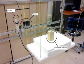
(a)

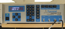
(b)

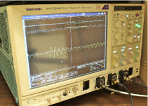
(c)

Figure 1: a) A photograph explaining our data collection process. The distance between the target (wooden block) and the measurement plane is about 0.8 m, which is about 26 wave lengths. b) Picosecond Pulse Generator. c) Textronix Oscilloscope.

3.1 Data collection

Figure 1-a) is a photograph explaining the data collection. The data collection is done in a regular room, which contains office furniture, computers, etc. Keeping in mind our desired application (see Introduction), we intentionally did not arrange a special waveguide, which would protect our data from unwanted signals caused by reflections from various objects in the room. Below $x$ and $y$ are horizontal and vertical axis respectively and the $z$ axis is perpendicular to the measurement plane, the positive direction of $z$ axis is in the direction from the target to the measurement plane. We dimensionalize our coordinates as $\mathbf{x}^{\prime}=\mathbf{x}/(1m),$ where “m” stands for meter. However, we do not change notations of coordinates for brevity. Hence, below, e.g. 0.05 of length actually means 5 centimeters.

”The transmitter sends the pulse into the medium which contains targets of interest. The electric wave caused by the pulse is scattered by the targets, and the backscattered signal is detected by the detector. The detected signal is recorded by the real time oscilloscope.”

Two main pieces of our device are Picosecond Pulse Generator (Figure 1-b)) and Textronix Oscilloscope (Figure 1-c)). The Picosecond Pulse Generator generates electric pulses. The duration of each pulse is 300 picoseconds. This pulse goes to the transmitter, which is a horn antenna (source).

The transmitter sends the pulse into the medium which contains targets of interest. The electric wave caused by the pulse is scattered by the targets, and the backscattered signal is detected by the detector. The detected signal is recorded by the real time oscilloscope. The oscilloscope produces a digitized time resolved signal with the step size in time of 10 picoseconds. The total time of measurements for one pulse is 10 nanoseconds=10⁴ picoseconds=10^-8 second.

To decrease the measurement noise, the pulse is generated 800 times for each position of the detector, the backscattering signal is also measured 800 times and resulting signals are averaged. The detector moves in both horizontal and vertical directions covering the square $SQ=\left\{-0.5<x,y<0.5\right\}$ on the measurement plane. We have chosen the step size of this movement to be 0.02. Although we can choose any step size, we found that 0.02 provides a good compromise between the precision of measurements and the total time spent on data collection.

The distance between our targets and the measurement plane is approximately 0.8 with about 0.05 deviations, and the wavelength of our signal is about 0.03. Therefore, the distance between the measurement plane and our targets is of about 26 wavelengths. This is in the far field zone.

3.2 Data pre-processing

The main difficulty working with experimental data is that there is a huge mismatch between these data and computationally simulated ones. Indeed, Figure 2-a) depicts a sample of experimentally measured data for a wooden block at one position of the detector, see Figure 1-a) for data collection scheme. On this figure, the direct signal is the signal going directly to the receiver. We use this direct signal as the time reference for data pre-processing. Unwanted signals are due to reflections of the electric wave from several objects present in the room. Figure 2-b) presents the computationally simulated data for the same target, see section 7.1 for data simulations. These figures show a huge mismatch between real and computationally simulated data. Therefore, data pre-processing is necessary. We refer to [15] for details of our data pre-processing procedure. The main steps of this procedure include:

1. Time-zero correction. The time-zero correction is to shift the measured data in time. So that its starting time is the same as when the incident pulse is emitted from the transmitter. This is done using the direct signals from the transmitter to the detector as the time reference.

2. Extraction of scattered signals. Apart from the backscattered wave by the targets, our measured data also contain various types of signals, e.g. direct signals from the horn to the detector, scattered signals from structures inside the room, etc. What we need, however, is the scattered signals by the targets only. To obtain them, we single out the scattered signals caused by the targets only and remove all unwanted signals.

3. Data propagation. After getting the scattered signals, the next step of data pre-processing is to propagate the data closer to the targets, i.e. to approximate the scattered wave on a plane which is much closer to the targets then the measurement plane. The distance between that propagated plane and the front surface of a target is usually between 0.02 and 0.06 (compare with the 0.8 distance from the measurement plane). There are two reasons for doing this. The first one is that the method of [3] works with the Laplace transform of the function $u\left(\mathbf{x},t\right)$ (section 4). That Laplace transform decays exponentially in terms of the time delay, which is proportional to the distance from the target to the measurement plane. Hence, the amplitude of the Laplace transformed experimental data on the measurement plane is very small and can be dominated by computational round-off error. The second reason is that this propagation procedure helps to substantially reduce the computational cost since the computational domain for the inverse problem is reduced.

4. Data calibration. Finally, since the amplitudes of the experimental incident and scattered waves are usually significantly different from simulations, we need to bring the former to the same level of the amplitude as the latter. This is done using a known target referred to as calibrating object.

In this paper, the result of data pre-processing is used as the measured data $g\left(\mathbf{x},t\right)$ on the backscattering boundary $\Gamma$ of our computational domain $\Omega$ for the inverse problem.

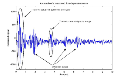
(a)

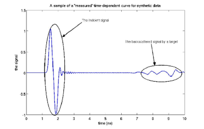
(b)

Figure 2: Typical samples of real and computationally simulated data. a) The measured data at one of detectors. The direct signal goes from the transmitter (Fig. 1-b)) to the detector because the transmitter emits the electric field in all directions. We use the direct signal as the time reference in our data pre-processing procedure. Unwanted signals are due to reflections from a variety of objects in the room. b) The computationally simulated data for the same target as the one of a) and at the same detector. A significant difference between a) and b) is evident.

4 The Approximately Globally Convergent Method in Brief

In this section we briefly outline the globally convergent method for reader’s convenience. We refer to sections 2.3, 2.5, 2.6.1 and 2.9.2 of [3] as well as [4] for details.

The first step of our inverse algorithm is the Laplace transform of the function $u\left(\mathbf{x},t\right),$

$$w(\mathbf{x},s)=\int\limits_{0}^{\infty}u(\mathbf{x},t)e^{-st}dt,\text{ for }s>\underline{s}=const.>0,$$ (6)

where $\underline{s}$ is a certain number. We assume that the number $\underline{s}$ is sufficiently large, and we call the parameter $s$ pseudo frequency. It follows from (1), (2) and (6) that the function $w$ is the solution of the following problem

$$\Delta w-s^{2}\varepsilon_{r}(\mathbf{x})w=-\delta\left(\mathbf{x}-\mathbf{x}_{0}\right),\text{ }x\in\mathbb{R}^{3},$$ (7)

$$\lim_{\left|x\right|\rightarrow\infty}w\left(\mathbf{x},s\right)=0.$$ (8)

The limit (8) is proved in Theorem 2.7.1 of [3]. In addition, it was proven in Theorem 2.7.2 of [3] that for the function $\varepsilon_{r}\left(\mathbf{x}\right)$ satisfying (3) there exists unique solution $w\left(\mathbf{x},s\right)$ of the problem (7), (8) for every $s>0$ such that

$$w\left(\mathbf{x},s\right)=w_{0}\left(\mathbf{x},s\right)+\overline{w}\left(\mathbf{x},s\right),\overline{w}\left(\mathbf{x},s\right)\in C^{2+\alpha}\left(\mathbb{R}^{3}\right),$$

where $w_{0}\left(\mathbf{x},s\right)$ is the solution of the problem (7), (8) for the case $\varepsilon_{r}(\mathbf{x})\equiv 1,$

$$w_{0}\left(\mathbf{x},s\right)=\frac{\exp\left(-s\left|\mathbf{x}-\mathbf{x}_{0}\right|\right)}{4\pi\left|\mathbf{x}-\mathbf{x}_{0}\right|}.$$

4.1 The integral differential equation

It follows from Theorem 2.7.2 of [3] that $w(\mathbf{x},s)>0.$ Hence, we can consider the functions $v(\mathbf{x},s)$, $q(\mathbf{x},s),$

$$v\left(\mathbf{x},s\right)=\frac{\ln w\left(\mathbf{x},s\right)}{s^{2}},\ q\left(\mathbf{x},s\right)=\frac{\partial v\left(\mathbf{x},s\right)}{\partial s}.$$ (9)

Substituting $w=\exp\left(s^{2}v\right)$ in (7) and keeping in mind that the source $\mathbf{x}_{0}\notin\overline{\Omega}$, we obtain

$$\Delta v+s^{2}|\nabla v|^{2}=\varepsilon_{r}(\mathbf{x}),\mathbf{x}\in\Omega.$$ (10)

Using (9) we obtain

$$v\left(\mathbf{x},s\right)=-\int\limits_{s}^{\overline{s}}q\left(\mathbf{x},\tau\right)d\tau+V\left(\mathbf{x},\overline{s}\right),$$ (11)

where the truncation pseudo frequency $\overline{s}>\underline{s}$ is a large number, which is chosen numerically, see section 8 for details. We call $V\left(\mathbf{x},\overline{s}\right)$ the tail function, and it is unknown. It follows from (9) and (11) that

$$V\left(\mathbf{x},\overline{s}\right)=v\left(\mathbf{x},\overline{s}\right)=\frac{\ln w\left(\mathbf{x},\overline{s}\right)}{\overline{s}^{2}}.$$ (12)

It follows from [3] (section 2.3) that, under some conditions, there exists a function $p\left(\mathbf{x}\right)\in C^{2+\alpha}\left(\overline{\Omega}\right)$ such that the following asymptotic behavior with respect to $\overline{s}\rightarrow\infty$ holds for functions $V$ and $q$

$$V\left(\mathbf{x},\overline{s}\right)=\frac{p\left(\mathbf{x}\right)}{\overline{s}}+O\left(\frac{1}{\overline{s}^{2}}\right),\text{ }\overline{s}\rightarrow\infty,$$ (13)

$$q\left(\mathbf{x},\overline{s}\right)=\partial_{\overline{s}}V\left(\mathbf{x},\overline{s}\right)=-\frac{p\left(\mathbf{x}\right)}{\overline{s}^{2}}+O\left(\frac{1}{\overline{s}^{3}}\right),\text{ }\overline{s}\rightarrow\infty.$$ (14)

Differentiating both sides of equation (10) with respect to $s$ then using (9) and (11), we obtain the following nonlinear integral differential equation

$$\begin{split}&\Delta q-2s^{2}\nabla q\int\limits_{s}^{\overline{s}}\nabla q\left(\mathbf{x},\tau\right)d\tau+2s\left(\int\limits_{s}^{\overline{s}}\nabla q\left(\mathbf{x},\tau\right)d\tau\right)^{2}\\ &+2s^{2}\nabla q\nabla V-4s\nabla V\int\limits_{s}^{\overline{s}}\nabla q\left(\mathbf{x},\tau\right)d\tau+2s\left(\nabla V\right)^{2}=0,\mathbf{x}\in\Omega,s\in\left[\underline{s},\overline{s}\right].\end{split}$$ (15)

In addition, (4) and (9) lead to the following Dirichlet boundary condition for the function $q$

$$q\left(\mathbf{x},s\right)=\widetilde{\psi}\left(\mathbf{x},s\right),\text{ }\forall\left(\mathbf{x},s\right)\in\Gamma\times\left[\underline{s},\overline{s}\right],$$ (16)

$$\widetilde{\psi}\left(\mathbf{x},s\right)=\frac{\partial_{s}\left(\ln\varphi\right)}{s^{2}}-2\frac{\ln\varphi}{s^{3}}.$$ (17)

Here $\varphi\left(\mathbf{x},s\right)$ is the Laplace transform (6) of the function $g\left(\mathbf{x},t\right)$ in (4). We now need to complement the boundary data (16) at the backscattering side $\Gamma$ with the boundary data at the rest of the boundary $\partial\Omega.$ Using computationally simulated data, it was shown numerically in section 6.8.5 of [3] as well as in [4] that it is reasonable to approximate the boundary data on $\partial\Omega\setminus\Gamma$ by the solution of the forward problem for the homogeneous medium for the case $\varepsilon_{r}\left(\mathbf{x}\right)=1$: recall that this equality holds outside of the domain $\Omega,$ see (3). Thus, we use below the following Dirichlet boundary condition for the function $q\left(\mathbf{x},s\right)$

$$q\left(\mathbf{x},s\right)=\psi\left(\mathbf{x},s\right),\text{ }\forall\left(\mathbf{x},s\right)\in\partial\Omega\times\left[\underline{s},\overline{s}\right],$$ (18)

$$\psi\left(\mathbf{x},s\right)=\left\{\begin{array}[]{c}\widetilde{\psi}\left(\mathbf{x},s\right),\text{ }\forall\left(\mathbf{x},s\right)\in\Gamma\times\left[\underline{s},\overline{s}\right],\\ \psi^{0}\left(\mathbf{x},s\right),\forall\left(\mathbf{x},s\right)\in\left(\partial\Omega\setminus\Gamma\right)\times\left[\underline{s},\overline{s}\right].\end{array}\right.$$ (19)

where the function $\psi^{0}\left(\mathbf{x},s\right)$ is the function $\widetilde{\psi}\left(\mathbf{x},s\right)$ in (17) computed for the case $\varepsilon_{r}(\mathbf{x})\equiv 1$.

Even though equation (15) with the boundary condition (18) has two unknown functions $q$ and $V$, we can approximate both of them because approximation procedures for them are different, see section 7.1. Suppose for a moment that functions $q$ and $V$ are approximated in $\Omega$ together with their derivatives $D_{\mathbf{x}}^{\alpha}q,D_{\mathbf{x}}^{\alpha}V,\left|\alpha\right|\leq 2.$ Then the corresponding approximation for the coefficient $\varepsilon_{r}(\mathbf{x})$ can be found via backwards calculation using (10).

4.2 The first approximation for the tail function

To start iterations, we need the first approximation $V_{1,0}\left(\mathbf{x}\right)$ for the tail function. In this section we show how to calculate $V_{1,0}\left(\mathbf{x}\right).$ This is the same choice as the one in section 2.9.2 of the book [3] as well as in [4].

Let the function $\varepsilon_{r}^{\ast}(\mathbf{x})$ satisfying (3) be the exact solution of our CIP for the exact data $g^{\ast}$ in (4). Let $V^{\ast}\left(\mathbf{x},\overline{s}\right)$ be the exact “tail function” defined as

$$V^{\ast}\left(\mathbf{x},\overline{s}\right)=\frac{\ln w^{\ast}\left(\mathbf{x},\overline{s}\right)}{\overline{s}^{2}}.$$ (20)

Let $q^{\ast}\left(\mathbf{x},s\right)\in C^{2+\alpha}\left(\overline{\Omega}\right)\times C\left[\underline{s},\overline{s}\right]$ be the corresponding exact function $q\left(\mathbf{x},s\right)$ satisfying equation (15). Let $\psi^{\ast}\left(\mathbf{x},s\right)\in C^{2+\alpha}\left(\overline{\Omega}\right)\times C\left[\underline{s},\overline{s}\right]$ be the corresponding exact Dirichlet boundary condition for $q^{\ast}\left(\mathbf{x},s\right)$ as defined in (18). Following (19), we assume that $\psi^{\ast}\left(\mathbf{x},s\right)=\psi^{0}\left(\mathbf{x},s\right)$ for $\left(\mathbf{x},s\right)\in\left(\partial\Omega\setminus\Gamma\right)\times\left[\underline{s},\overline{s}\right].$Hence, (15) and (18) hold for functions $q^{\ast},\psi^{\ast}.$ Setting in (15) $s=\overline{s},$ we obtain

$$\begin{split}\Delta q^{\ast}+2\overline{s}^{2}\nabla q^{\ast}\nabla V^{\ast}+2\overline{s}\left(\nabla V^{\ast}\right)^{2}&=0,~{}~{}\mathbf{x}\in\Omega,\\ q^{\ast}\mid_{\partial\Omega}&=\psi^{\ast}\left(\mathbf{x},\bar{s}\right),~{}\mathbf{x}\in\partial\Omega.\end{split}$$ (21)

Next, truncating the second term in each of the asymptotics (13) and (14), we obtain that there exists a function $p^{\ast}\left(\mathbf{x}\right)\in C^{2+\alpha}\left(\overline{\Omega}\right)$ such that

$$\begin{split}V^{\ast}\left(\mathbf{x},\overline{s}\right)&\approx\frac{p^{\ast}\left(\mathbf{x}\right)}{\overline{s}},\text{ }\overline{s}\rightarrow\infty,\\ q^{\ast}\left(\mathbf{x},\overline{s}\right)&=\partial_{\overline{s}}V^{\ast}\left(\mathbf{x},\overline{s}\right)\approx-\frac{p^{\ast}\left(\mathbf{x}\right)}{\overline{s}^{2}},\text{ }\overline{s}\rightarrow\infty.\end{split}$$ (22)

Substituting formulae (22) into (21), we obtain the following approximate Dirichlet boundary value problem for the function $p^{\ast}\left(x\right)$

$$\Delta p^{\ast}=0\text{ in }\Omega,\text{ }p^{\ast}\in C^{2+\alpha}\left(\overline{\Omega}\right),$$ (23)

$$p^{\ast}|_{\partial\Omega}=-\overline{s}^{2}\psi^{\ast}\left(\mathbf{x},\overline{s}\right).$$ (24)

Thus, using (20) and (22), we obtain the following approximate mathematical model.

Approximate mathematical model.

We assume that there exists a function $p^{\ast}\left(x\right)\in C^{2+\alpha}\left(\overline{\Omega}\right)$ such that the exact tail function $V^{\ast}\left(\mathbf{x},s\right)$ has the form

$$V^{\ast}\left(\mathbf{x},s\right)=\frac{p^{\ast}\left(\mathbf{x}\right)}{s}=\frac{\ln w^{\ast}\left(\mathbf{x},s\right)}{s^{2}},\text{ }\forall s\geq\overline{s},\text{ }$$ (25)

and the function $q^{\ast}\left(\mathbf{x},\overline{s}\right)$ is

$$q^{\ast}\left(\mathbf{x},\overline{s}\right)=-\frac{p^{\ast}\left(\mathbf{x}\right)}{\overline{s}^{2}}\text{.}$$

Because of (23), (24) and (25), we set for the first tail

$$V_{1,0}\left(\mathbf{x}\right)=\frac{p\left(\mathbf{x}\right)}{\overline{s}},$$ (26)

where the function $p(\mathbf{x})$ is the solution of the following Dirichlet boundary value problem

$$\Delta p=0\text{ in }\Omega,\text{ }p\in C^{2+\alpha}\left(\overline{\Omega}\right),$$ (27)

$$p|_{\partial\Omega}=-\overline{s}^{2}\psi\left(\mathbf{x},\overline{s}\right).$$ (28)

We point out that we calculate $V_{1,0}\left(\mathbf{x}\right)$ without any advanced knowledge of a small neighborhood of the exact coefficient $\varepsilon_{r}^{\ast}(\mathbf{x}).$ Using (22)-(28) and Schauder theorem [14], we obtain

$$\left\|V_{1,0}\left(\mathbf{x}\right)-V^{\ast}\left(\mathbf{x},\overline{s}\right)\right\|_{C^{2+\alpha}\left(\overline{\Omega}\right)}\leq C\overline{s}\left\|\psi^{\ast}\left(\mathbf{x},\overline{s}\right)-\psi\left(\mathbf{x},\overline{s}\right)\right\|_{C^{2+\alpha}\left(\partial\Omega\right)},$$ (29)

where the number $C=C\left(\Omega\right)>0$ depends only from the domain $\Omega.$ Hence, the error in the calculation of $V_{1,0}\left(\mathbf{x}\right)$ depends only on the error in the boundary data $\psi\left(\mathbf{x},\overline{s}\right).$ On the other hand, since the boundary function $\psi\left(\mathbf{x},s\right)$ is generated by the function $g(\mathbf{x},t)$ in (4), then the error in $\psi\left(\mathbf{x},\overline{s}\right)$ is generated by the error in measurements. The estimate (29) is one of elements of the proof of the approximate global convergence theorem for this numerical method, see Theorem 2.9.4 in [3] and Theorem 5.1 in [4]. Although a good approximation for the exact solution $\varepsilon_{r}^{\ast}(\mathbf{x})$ can be derived from the function $V_{1,0}\left(\mathbf{x}\right),$ we have observed computationally that better approximations are delivered via iterations described below in sections 6.1, 6.2.

4.3 Discretization with respect to the pseudo-frequency

To approximate both functions $q$ and $V$ using (15) and (18), we consider the layer stripping procedure with respect to $s$. We divide the interval $\left[\underline{s},\overline{s}\right]$ into $N$ small subintervals with the uniform step size $h=s_{n-1}-s_{n}$. Here, $\underline{s}=s_{N}<s_{N-1}<...<s_{0}=\overline{s}.$ We approximate the function $q(\mathbf{x},s)$ as a piecewise constant function with respect to $s,$ i.e. we assume that $q(\mathbf{x},s)=q_{n}(\mathbf{x})$ for $s\in\left[s_{n},s_{n-1}\right).$ Hence, using (11), we approximate the function $v\left(\mathbf{x},s_{n}\right)$ as

$$v\left(\mathbf{x},s_{n}\right)=-h\sum\limits_{j=0}^{n}q_{j}\left(\mathbf{x}\right)+V\left(\mathbf{x},\overline{s}\right),q_{0}\left(\mathbf{x}\right):\equiv 0.$$ (30)

To obtain a sequence of Dirichlet boundary value problems for elliptic PDEs for functions $q_{n}(\mathbf{x}),$ we introduce the $s-$dependent Carleman Weight Function (CWF) $\mathcal{C}_{n,\mu}\left(s\right)=\exp\left[\mu\left(s-s_{n-1}\right)\right],$ where $\mu>>1$ is a large parameter. In our numerical studies we take $\mu=20$. This function mitigates the influence of the nonlinear term in the resulting integral-differential equations on every pseudo-frequency interval $\left(s_{n},s_{n-1}\right)$.

Multiply both sides of equation (15) by $\mathcal{C}_{n,\mu}\left(s\right)$ and integrate with respect to $s\in\left(s_{n},s_{n-1}\right).$ We obtain

$$\begin{split}&\Delta q_{n}-A_{1,n}\left(h\sum\limits_{j=0}^{n-1}\nabla q_{j}-\nabla V_{n}\right)\nabla q_{n}\\ &=B_{n}\left(\nabla q_{n}\right)^{2}-A_{2,n}h^{2}\left(\sum\limits_{j=0}^{n-1}\nabla q_{j}\right)^{2}+2A_{2,n}\nabla V_{n}\left(h\sum\limits_{j=0}^{n-1}\nabla q_{j}\right)-A_{2,n}\left(\nabla V_{n}\right)^{2},\\ &q_{n}\left(\mathbf{x}\right)\mid_{\partial\Omega}=\psi_{n}(\mathbf{x}):=\frac{1}{h}\int\limits_{s_{n}}^{s_{n-1}}\psi\left(\mathbf{x},s\right)ds,\text{ }n=1,...,N.\end{split}$$ (31)

Here $V_{n}\left(\mathbf{x}\right)$ is such an approximation of the tail function $V\left(\mathbf{x}\right)$ which corresponds to the function $q_{n}\left(\mathbf{x}\right)$ (section 6.1). Numbers $A_{1,n},A_{2,n},B_{n}$ are computed explicitly. Furthermore, $B_{n}=O\left(1/\mu\right),\mu\rightarrow\infty.$ For this reason we ignore the nonlinear term in (31), thus setting

$$B_{n}\left(\nabla q_{n}\right)^{2}:=0.$$ (32)

Note that (32) is not a linearization, since (31) contains products $\nabla q_{j}\nabla q_{i}$ and also because the tail function $V_{n}$ depends nonlinearly on functions $q_{j},$ see (12) and step 6 in section 6.1.

5 A Finite Element Method for the Reconstruction of $\varepsilon_{r}\left(\mathbf{x}\right)$

In this section we explain how we compute functions $\varepsilon_{rn}(\mathbf{x})$ on every pseudo-frequency interval $\left(s_{n},s_{n-1}\right)$ using the FEM. Once the functions $q_{j},j=1,...n$ along with the function $V_{n}$ in (31) are calculated, we compute the function $v_{n}\left(\mathbf{x}\right)$ using the direct analog of (30),

$$v_{n}\left(\mathbf{x}\right)=-h\sum\limits_{j=0}^{n}q_{j}\left(\mathbf{x}\right)+V_{n}\left(\mathbf{x}\right),\text{ }x\in\Omega.$$

Using (9), we set

$$w_{n}\left(\mathbf{x}\right)=\exp\left[s_{n}^{2}v_{n}\left(\mathbf{x}\right)\right].$$ (33)

To find the function $\varepsilon_{rn}\left(\mathbf{x}\right),$ we note that the function $w_{n}\left(\mathbf{x},s_{n}\right)$ is the solution of the following analog of the problem (7), (8)

$$\Delta w_{n}-s_{n}^{2}\varepsilon_{rn}\left(\mathbf{x}\right)w_{n}=0\text{ in }\Omega,$$ (34)

$$\partial_{n}w_{n}\mid_{\partial\Omega}=f_{n}\left(\mathbf{x}\right),$$ (35)

where

$$f_{n}\left(\mathbf{x}\right)=\partial_{n}\exp\left[s_{n}^{2}v_{n}\left(\mathbf{x}\right)\right]\text{ for }\mathbf{x}\in\partial\Omega.$$ (36)

To compute the function $\varepsilon_{rn}\left(\mathbf{x}\right)$ from (34), (35) and (36), we apply a version of the FEM as described below in sections 5.1, 5.2.

5.1 Spaces of finite elements

Following [12] we discretize in computations our bounded domain $\Omega\subset\mathbb{R}^{3}$ by an unstructured tetrahedral mesh $T$ using non-overlapping tetrahedral elements $K\in\mathbb{R}^{3}$. The elements $K$ are such that $T=\{K_{1},...,K_{m}\}$, where $m$ is the total number of elements in $\Omega$, and

$$\Omega=\cup_{K\in T}K=K_{1}\cup K_{2}...\cup K_{m}.$$

We associate with the mesh $T$ the mesh function $h=h(\mathbf{x})$ as a piecewise-constant function such that

$$h(\mathbf{x})=h_{K},~{}\forall K\in T,$$

where $h_{K}$ is the diameter of $K$ which we define as the longest side of $K$. We impose the following shape regularity assumption of the mesh $T$ for every element $K\in T$

$$a_{1}\leq h_{K}\leq r^{\prime}a_{2},\quad a_{1},a_{2}=const.>0,$$ (37)

where $r^{\prime}$ is the radius of the maximal sphere contained in the element $K$.

Define the set of polynomials $P_{r}(K)$ as

$$P_{r}(K)=\big{\{}v:v(x,y,z)=\sum_{0\leq i+j+l\leq r}c_{ijl}x^{i}y^{j}z^{l},(x,y,z)\in K,c_{ijl}\in\mathbb{R},~{}\forall K\in T\big{\}}.$$ (38)

We introduce now the finite element space $V_{h}$ as

$$V_{h}=\big{\{}v(x)\in H^{1}\left(\Omega\right):v\in C(\Omega),~{}v|_{K}\in P_{1}(K)~{}\forall K\in T\big{\}},$$

where $P_{1}(K)$ denotes the set of linear functions on $K$ defined by (38) for $r=1$. Hence, the finite element space $V_{h}$ consists of continuous piecewise linear functions in $\Omega$. To approximate functions $\varepsilon_{rn},$ we introduce the space of piecewise constant functions $C_{h}$,

$$C_{h}:=\{u\in L_{2}(\Omega):u|_{K}\in P_{0}(K),\forall K\in T\},$$

where $P_{0}(K)$ is the piecewise constant function on $K$ defined by (38) for $r=0$.

5.2 A finite element method

To compute the function $\varepsilon_{rn}$ from (34), we formulate the finite element method for the problem (35)-(36) as: Find the function $\varepsilon_{rn}\in C_{h}$ for the known function $w_{n}\in V_{h}$ such that

$$(\varepsilon_{rn}w_{n},v)=-\frac{1}{s_{n}^{2}}(\nabla w_{n},\nabla v)+\frac{1}{s_{n}^{2}}(f_{n},v)_{\partial\Omega},\forall v\in V_{h},$$ (39)

where $(\cdot,\cdot)$ is the scalar product in $L_{2}\left(\Omega\right)$.

We expand $w_{n}$ in terms of the standard continuous piecewise linear functions $\{\varphi_{l}\}_{l=1}^{P}$ in the space $V_{h}$ as

$$w_{n}(\mathbf{x})=\sum_{l=1}^{P}w_{n,l}\varphi_{l}(\mathbf{x}),$$ (40)

where $w_{n,l}$ denote the nodal values of the function $w_{n}$ at the nodes $l$ of the elements $K$ in the mesh $T$. We can determine $w_{n,l}$ by knowing already computed functions $v_{n,l}$ using the following analog of (33)

$$w_{n}\left(\mathbf{x}\right)=\exp\left[s_{n}^{2}v_{n,l}\left(\mathbf{x}\right)\right],\forall\mathbf{x}\in\Omega.$$

Substitute (40) into (39) and choose $v(\mathbf{x})=\varphi_{j}(\mathbf{x}).$ Then we obtain the following linear algebraic system of equations

$$\sum_{l,j=1}^{P}\varepsilon_{rn,l}(w_{n,l}\varphi_{l},\varphi_{j})=-\frac{1}{s_{n}^{2}}\sum_{l,j=1}^{P}w_{n,l}(\nabla\varphi_{l},\nabla\varphi_{j})+\frac{1}{s_{n}^{2}}\sum_{j=1}^{P}\left[f_{n},\varphi_{j}\right],$$ (41)

where $\left[\cdot,\cdot\right]$ is the scalar product in $L_{2}\left(\partial\Omega\right).$ The system (41) can be rewritten in the matrix form for the unknown vector $\varepsilon_{rn}=\left\{\varepsilon_{rn,l}\right\}_{l=1}^{P}$ and known vector $w_{n}=\left\{w_{n,l}\right\}_{l=1}^{P}$ as

$$M\varepsilon_{rn}=-\frac{1}{s_{n}^{2}}Gw_{n}+\frac{1}{s_{n}^{2}}F.$$ (42)

Here $M$ is the block mass matrix in space, $G$ is the stiffness matrix corresponding to the term containing $(\nabla\varphi_{l},\nabla\varphi_{j})$ in (41) and $F$ is the load vector. At the element $K$ the matrix entries in (42) are explicitly given by:

$$M_{l,j}^{K}=(w_{n,l}~{}\varphi_{l},\varphi_{j})_{K},G_{l,j}^{K}=(\nabla\varphi_{l},\nabla\varphi_{j})_{K},F_{n,j}^{K}=(f_{n},\varphi_{j})_{K}.$$

To obtain an explicit scheme for the computation of coefficients $\varepsilon_{rn}$, we approximate the matrix $M$ by the lumped mass matrix $M^{L}$ in space, i.e., the diagonal approximation is obtained by taking the row sum of $M$ [3]. We obtain

$$\varepsilon_{rn}=-\frac{1}{s_{n}^{2}}(M^{L})^{-1}Gw_{n}+\frac{1}{s_{n}^{2}}(M^{L})^{-1}F.$$ (43)

Note that for the case of linear Lagrange elements which are used in our computations in section 8 we have $M=M^{L}$. Thus, the lumping procedure does not include approximation errors in this case.

6 The Approximately Globally Convergent Algorithm

We present now our algorithm for the numerical solution of equations (31) and computing the functions $\varepsilon_{rn}$ using the equation(43). In this algorithm the index $i$ denotes the number of inner iterations inside every pseudo-frequency interval $\left(s_{n},s_{n-1}\right)$ when we update tails.

6.1 The algorithm

Step 0

Set $q_{0}=0$. Compute the initial tail function $V_{1,0}(\mathbf{x},\overline{s})\in C^{2+\alpha}(\overline{\Omega})$ as in (26)-(28).

Step 1

Here we describe iterations which update tails inside every pseudo-frequency interval $\left(s_{n},s_{n-1}\right)$. Let $n\geq 1,i\geq 1.$ Suppose that functions $q_{j},j=1,...,n-1,V_{n,i-1}$ are computed. Solve the Dirichlet boundary value problem for the function $q_{n,i}\left(\mathbf{x}\right)\in C^{2+\alpha}\left(\overline{\Omega}\right),$

$$\begin{split}\Delta q_{n,i}-A_{1n}&\left(h\sum\limits_{j=1}^{n-1}\nabla q_{j}\right)\cdot\nabla q_{n,i}+A_{1n}\nabla q_{n,i}\cdot\nabla V_{n,i-1}=\\ &-A_{2n}h^{2}\left(\sum\limits_{j=1}^{n-1}\nabla q_{j}\right)^{2}+2A_{2n}\nabla V_{n,i-1}\cdot\left(h\sum\limits_{j=1}^{n-1}\nabla q_{j}\right)-A_{2n}\left(\nabla V_{n,i-1}\right)^{2},\\ q_{n,i}\left(\mathbf{x}\right)&=\psi_{n}\left(\mathbf{x}\right),\qquad\mathbf{x}\in\partial\Omega.\end{split}$$ (44)

Step 2

Compute functions $v_{n,i}\left(\mathbf{x}\right)$ and $w_{n,i}\left(\mathbf{x}\right),$

$$v_{n,i}\left(\mathbf{x}\right)=-hq_{n,i}\left(\mathbf{x}\right)-h\sum\limits_{j=0}^{n-1}q_{j}\left(\mathbf{x}\right)+V_{n,i}\left(\mathbf{x}\right),$$

$$w_{n,i}\left(\mathbf{x}\right)=\exp\left[s_{n}^{2}v_{n,i}\left(\mathbf{x}\right)\right].$$

Step 3

Compute the function $\overline{\varepsilon}_{r,n,i}\in C_{h}$ via backwards calculations, using the finite element formulation of equation (43) as

$$\overline{\varepsilon}_{rn,i}\left(\mathbf{x}\right)=-\frac{1}{s_{n}^{2}}(M^{L})^{-1}Gw_{n,i}+\frac{1}{s_{n}^{2}}(M^{L})^{-1}F.$$

Since by (3) we should have $\varepsilon_{r}\left(\mathbf{x}\right)\geq 1,\forall\mathbf{x}\in\mathbb{R}^{3},$ and also since we need to extend the function $\overline{\varepsilon}_{r,n,i}\left(\mathbf{x}\right)$ outside of the domain $\Omega$ by unity, we set

$$\varepsilon_{rn,i}\left(\mathbf{x}\right)=\left\{\begin{array}[]{c}\overline{\varepsilon}_{rn,i}\left(\mathbf{x}\right)\text{ if }\overline{\varepsilon}_{r,n,i}\left(\mathbf{x}\right)\geq 1,\\ 1\text{ if either }\overline{\varepsilon}_{rn,i}\left(\mathbf{x}\right)<1,\text{ or }\mathbf{x}\in\mathbb{R}^{3}\diagdown\Omega.\end{array}\right.$$ (45)

Step 4

Solve the forward problem (1)-(2) with ${\varepsilon_{r}}(\mathbf{x}):=\varepsilon_{rn,i}\left(\mathbf{x}\right)$ and compute the Laplace transform (6) for $s=s_{n}$. We obtain the function $w_{n,i}\left(\mathbf{x},s_{n}\right)$.

Step 5

Update the tail function as

$$V_{n,i}(\mathbf{x})=\frac{\ln w_{n,i}\left(\mathbf{x},s_{n}\right)}{{s_{n}}^{2}}.$$ (46)

Continue inner iterations with respect to $i$ until the stopping criterion of Step 1 of section 6.2 is met at $i=m_{n}$.

Step 6

Set for the pseudo-frequency interval $[s_{n},s_{n-1})$

$$q_{n}(\mathbf{x}):=q_{n,m_{n}}(\mathbf{x}),{\varepsilon}_{rn}(\mathbf{x}):={\varepsilon}_{rn,m_{n}}(\mathbf{x}),V_{n+1,0}\left(\mathbf{x}\right):=\frac{\ln w_{n,m_{n}}\left(\mathbf{x},s_{n}\right)}{{s_{n}}^{2}}:=V_{n}\left(\mathbf{x}\right).$$ (47)

Step 7

If either the stopping criterion with respect to $n$ of Step 4 of section 6.2 is met, or $n=N,$ then set the resulting function ${\varepsilon}_{rn}(\mathbf{x})$ as the solution of our CIP. Otherwise, set $n:=n+1$ and go to Step 1.

6.2 The stopping criterion

When testing the algorithm of section 6.1 on experimental data, we have developed a reliable stopping criterion for iterations $(n,i)$ in this algorithm. On every pseudo-frequency interval $\left(s_{n},s_{n-1}\right)$ we define “first norms” $D_{n,0}$ as

$$D_{n,0}=||{V}_{n,0}-\tilde{V}_{n}||_{L_{2}(\Omega)}.$$ (48)

In (48) the function ${V}_{n,0}$ is the computed tail functions at the inner iteration $i=0$ as in (47). Functions $\tilde{V}_{n}$ in (48) are obtained from the known measured function $g(\mathbf{x},t)$ in (4) as

$$\tilde{V}_{n}\left(\mathbf{x}\right)=\frac{\ln W(\mathbf{x},{s_{n}})}{s_{n}^{2}},$$ (49)

where $W(\mathbf{x},s_{n})$ is the Laplace transform of the function $g(\mathbf{x},t)$ at $s=s_{n}$.

We have observed that computed “first norms” $D_{n,0}$ always achieve only one minimum at a certain $n=\overline{n}$, where the number $\overline{n}$ depends on the specific set of experimental data. Furthermore, in non-blind cases of non-metallic targets, the corresponding values of $\max_{\overline{\Omega}}{\varepsilon_{r\overline{n},0}}(\mathbf{x})$ were in a good agreement with a priori known ones. However, in the cases of non-blind metallic targets we have observed that $5\leq\max_{\overline{\Omega}}{\varepsilon_{r\overline{n},0}}(\mathbf{x})\leq 10.$ This contradicts with (5). Therefore, we have developed the following stopping criterion which consists of four steps.

The Stopping Criterion

The first step in our criterion is for stopping inner iterations with respect to $i$ in step 5 of section 6.1. As to Steps 2-4, they are for stopping outer iterations with respect to $n$ (Step 7 in section 6.1). First, we define numbers $B_{n,i}$ and $D_{n,i}$ as

$$B_{n,i}=\frac{||{\varepsilon_{rn,i}}-{\varepsilon_{rn,i-1}}||_{L_{2}(\Omega)}}{||{\varepsilon_{rn,i-1}}||_{L_{2}(\Omega)}},$$

$$D_{n,i}=||{V}_{n,i}-\tilde{V}_{n}||_{L_{2}(\Omega)},$$ (50)

In (50) functions ${V}_{n,i}$ are computed tail functions corresponding to ${\varepsilon_{rn,i}}$ (step 6 in section 6.1) and functions $\tilde{V}_{n}=\tilde{V}_{n}(\mathbf{x},s_{n})$ are calculated using (49).

• Step 1. Iterate with respect to $i$ and stop iterations at $i=m_{n}\geq 1$ such that

  $$\text{either }B_{n,i}\geq B_{n,i-1}\text{ or }B_{n,i}\leq\eta,$$ (51)

  or

  $$\text{either }\text{{}}D{{}_{n,i}}\geq D{{}_{n,i-1}}\text{ or }D{{}_{n,i}}\leq\eta,$$ (52)

  where $\eta=10^{-6}$ is a chosen tolerance.

• Step 2. For every $n$ compute “final norms” $D_{n,m_{n}}$ as

  $$D_{n,m_{n}}=||{V}_{n+1,0}-\tilde{V}_{n}||_{L_{2}(\Omega)}.$$ (53)

  In (53) functions ${V}_{n+1,0}\left(x\right)$ are computed as in (47).

• Step 3. Compute the number $\overline{N}$ of the pseudo frequency interval such that the first norms $D_{n,0}$ in (48) achieve its first minimum with respect to $n$ and get corresponding $\varepsilon_{r\overline{N},0}(\mathbf{x})$ on this interval. Compute the number $\overline{M}$ of the pseudo frequency interval such that the final norms $D_{n,m_{n}}$ in (53) achieve its first minimum or they are stabilized with respect to $n$, and get corresponding $\varepsilon_{r\overline{M},0}(\mathbf{x})$ on this interval. Next, compute the number $\tilde{\varepsilon}_{r},$

  $$\tilde{\varepsilon}_{r}=\left\{\begin{array}[]{cc}\max_{\overline{\Omega}}\varepsilon_{r\overline{M},0}\left(\mathbf{x}\right),&\text{ if }\overline{M}<\overline{N},\\ \max_{\overline{\Omega}}\varepsilon_{r\overline{N},0}\left(\mathbf{x}\right),&\text{ if }\overline{M}\geq\overline{N}.\end{array}\right.$$ (54)

• Step 4. If $\tilde{\varepsilon}_{r}<5$ or $\tilde{\varepsilon}_{r}>10,$ then take the final reconstructed value of the refractive index $n=\sqrt{\tilde{\varepsilon}_{r}}.$ As the computed function $\varepsilon_{r}\left(\mathbf{x}\right),$ take

  $$\varepsilon_{r,comp}\left(\mathbf{x}\right)=\left\{\begin{array}[]{cc}\varepsilon_{r\overline{M},0}\left(\mathbf{x}\right),&\text{ if }\overline{M}<\overline{N},\\ \varepsilon_{r\overline{N},0}\left(\mathbf{x}\right),&\text{ if }\overline{M}\geq\overline{N}.\end{array}\right.$$ (55)

  and stop iterations. However, if $5\leq\tilde{\varepsilon}_{r}\leq 10,$ then continue iterations and compute the number $\widetilde{N}\in\left(\overline{N}+1,N\right]$ of the pseudo frequency interval such that the global minimum with respect to $n$ of final norms $D_{n,m_{n}}$ in (53) is achieved. Then, similarly with (54), compute the number $\varepsilon_{r\widetilde{N}},$

  $$\varepsilon_{r\widetilde{N}}=\max_{\overline{\Omega}}\varepsilon_{r\widetilde{N},0}\left(\mathbf{x}\right)$$ (56)

  and take $n=\sqrt{\varepsilon_{r\widetilde{N}}}$ as the final reconstructed value of the refractive index. Also, take the function $\varepsilon_{r,comp}\left(\mathbf{x}\right)=\varepsilon_{r\widetilde{N},0}\left(\mathbf{x}\right)$ as the computed coefficient $\varepsilon_{r}\left(\mathbf{x}\right)$ and stop iterations.

We have observed in all our computations that conditions of our stopping criterion are always achieved. More precisely, one of conditions (51), (52) is always achieved for iterations with respect to $i$ and the minimal values mentioned in Steps 3 and 4 are always achieved. Figure 3 displays a typical $n-$dependence of sequences $D_{n,0\text{ }}$and $D_{n,m_{n}}.$

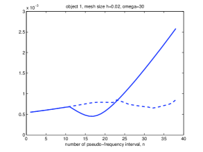
(a) a) Test 1

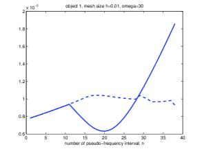
(b) b) Test 2

Figure 3: Behaviour of norms $D_{n,m_{n}}$ (solid curve) and $D_{n,m_{n}}$ (dashed curve) for object 1.

7 Some Details of the Numerical Implementation

In this section we present some additional details of our numerical implementation. Because of (5), we define in all our tests the upper value of the function $\varepsilon_{r}\left(\mathbf{x}\right)$ as $b=15,$ see (3). Thus, we set lower and upper bounds for the reconstructed function $\varepsilon_{r}(\mathbf{x})$ in $\Omega$ as

$$M_{\varepsilon_{r}}=\{\varepsilon_{r}(\mathbf{x}):\varepsilon_{r}\left(\mathbf{x}\right)\in\left[1,15\right]\}.$$ (57)

As to the lower bound, we ensure it via (45). We ensure the upper bound 15 similarly via truncating to 15 those values of $\varepsilon_{r,comp}\left(\mathbf{x}\right)$ which exceed this number. To solve Dirichlet boundary value problems (44), we use FEM. We reconstruct refractive indices rather than dielectric constants of material since they can be directly measured.

To compare our computational results with directly measured refractive indices $n=\sqrt{\varepsilon_{r}}$ of dielectric targets and with appearing dielectric constants of metallic targets (see (5)), we consider maximal values of computed functions $\varepsilon_{r,comp}\left(\mathbf{x}\right)$,

$$\varepsilon_{r}^{\text{comp}}=\max_{\overline{\Omega}}\varepsilon_{r,comp}\left(\mathbf{x}\right),n^{\text{comp}}=\sqrt{\varepsilon_{r}^{\text{comp}}},$$ (58)

see Step 4 of section 6.2 for the definition of $\varepsilon_{r,comp}\left(\mathbf{x}\right).$ Using experimental data for non-blind targets and comparing reconstruction results with cases of synthetic data, we have found that our algorithm provided accurate results with the following pseudo frequency interval, which we use in all our computations

$$s\in[8,10],\underline{s}=8,\overline{s}=10,h=0.05.$$

7.1 Computations of the forward problem

As it is clear from Step 4 of section 6.1, we need to solve the forward problem (1), (2) on each iterative step of inner iterations to update the tail via (46). Since it is impossible to computationally solve equation (1) in the infinite space $\mathbb{R}^{3},$ we work with a truncated domain. Namely, we choose the domain $G$ as

$$G=\left\{\mathbf{x=}(x,y,z)\in(-0.56,0.56)\times(-0.56,0.56)\times(-0.16,0.1)\right\}.$$

We use the hybrid FEM/FDM method described in [2] and the software package WavES [18]. We split $G$ into two subdomains $G_{FEM}=\Omega$ and $G_{FDM}$ so that $G=G_{FEM}\cup G_{FDM}$. We solve the forward problem in $G$ and the inverse problem via the algorithm of section 6.1 in $\Omega.$ The space mesh in $G_{FEM}$ and in $G_{FDM}$ consists of tetrahedral and cubes, respectively. Below

$$G_{FEM}=\Omega=\left\{\mathbf{x=}(x,y,z)\in(-0.5,0.5)\times(-0.5,0.5)\times(-0.1,0.04)\right\}.$$ (59)

Since by (3) $\varepsilon_{r}(\mathbf{x})=1$ in $G_{FDM},$ then it is computationally efficient to use FDM in $G_{FDM}$ and to use FEM in $G_{FEM}=\Omega,$ as it is done in the hybrid method of [2].

The front and back sides of the rectangular prism $G$ are $\{z=0.1\}$ and $\{z=-0.16\}$, respectively. The boundary of the domain $G$ is $\partial G=\partial_{1}G\cup\partial_{2}G\cup\partial_{3}G.$ Here, $\partial_{1}G$ and $\partial_{2}G$ are, respectively, front and back sides of the domain $G$, and $\partial_{3}G$ is the union of left, right, top and bottom sides of this domain. The front side $\Gamma$ of the rectangular prism $\Omega$ where the propagated data $g\left(\mathbf{x},t\right)$ in (4) are given, is

$$\Gamma=\{\mathbf{x}\in\partial\Omega:z=0.04\}$$ (60)

Now we describe the forward problem which is used in our computations. To compute tail functions $V_{n,i}$ via Steps 4, 5 of the algorithm of section 6.1, we computationally solve the following forward problem in our tests:

$$\begin{split}\varepsilon_{r}\left(\mathbf{x}\right)u_{tt}-\Delta u&=0,~{}~{}~{}\mbox{in}~{}G\times(0,T),\\ u(\mathbf{x},0)&=0,~{}u_{t}(\mathbf{x},0)=0,~{}\mbox{in}~{}G,\\ \partial_{n}u&=f\left(t\right),~{}\mbox{on}~{}\partial_{1}G\times(0,t_{1}],\\ \partial_{n}u&=-\partial_{t}u,~{}\mbox{on}~{}\partial_{1}G\times(t_{1},T),\\ \partial_{n}u&=-\partial_{t}u,~{}\mbox{on}~{}\partial_{2}G\times(0,T),\\ \partial_{n}u&=0,~{}\mbox{on}~{}\partial_{3}G\times(0,T),\end{split}$$ (61)

where $f(t)$ is the amplitude of the initialized plane wave,

$$f(t)=\sin\omega t,~{}0\leq t\leq t_{1}:=\frac{2\pi}{\omega}.$$

We use $\omega=30$ and $T=1.2.$ We solve the problem (61) using the explicit scheme with the time step size $\tau=0.003,$ which satisfies the CFL condition.

7.2 Two stages

Our reconstruction procedure is done in two stages described in this section.

7.2.1 First stage

In the first stage we follow the algorithm of section 6.1. We have observed that this stage provides accurate locations of targets of interest. It also provides accurate values of refractive indices $n=\sqrt{\varepsilon_{r\overline{N}}}$ of dielectric targets and large values of appearing dielectric constants $\varepsilon_{r\widetilde{N}}$ for metallic targets, see (54) and (56). However, the algorithm of section 6.1 does not reconstruct well sizes/shapes of targets. Thus, we need a postprocessing procedure, which is done in the second stage.

7.2.2 The second stage: postprocessing

Let $\varepsilon_{rn,i}\left(\mathbf{x}\right)$ be the function in (45). Then we set

$$\widetilde{\varepsilon}_{rn,i}(\mathbf{x})=\left\{\begin{array}[]{ll}\varepsilon_{rn,i}(\mathbf{x})&\text{ if }\varepsilon_{rn,i}(\mathbf{x})>0.5\max\limits_{\Omega}\varepsilon_{rn,i}(\mathbf{x}),\\ 1,&\text{ otherwise. }\end{array}\right.$$ (62)

Next, we determine minimal $x_{\min},y_{\min}$ and maximal $x_{\max},y_{\max}$ values in $x$ and $y$ directions, where the function $\widetilde{\varepsilon}_{rn,i}(\mathbf{x})>1.$ Next, we set

$$\varepsilon_{rn,i}\left(\mathbf{x}\right):=\begin{cases}\widetilde{\varepsilon}_{rn,i}(\mathbf{x})&\text{ if }x\in\left[x_{\min},x_{\max}\right],y\in\left[y_{\min},y_{\max}\right],\\ 1&\text{ otherwise}\end{cases}$$

and proceed with Step 5 of the algorithm of section 6.1. In this second stage we perform the same number of iterations with respect to both indices $n,i$ as ones of the first stage. We are concerned in the second stage only with sized and shapes of targets, and we are not concerned with values of $\varepsilon_{r}^{\text{comp}},n^{\text{comp}}.$ Rather, we take these values from the first stage. Let $\widetilde{\varepsilon}_{r}\left(\mathbf{x}\right)$ be the function $\varepsilon_{r}\left(\mathbf{x}\right)$ obtained at the last iteration of the second stage. Then we form the image of the target based on the function $\varepsilon_{r,image}\left(\mathbf{x}\right),$

$$\varepsilon_{r,image}\left(\mathbf{x}\right)=\left\{\begin{array}[]{l}\widetilde{\varepsilon}_{r}\left(\mathbf{x}\right)\text{ if }\widetilde{\varepsilon}_{r}\left(\mathbf{x}\right)\geq 0.9\max_{\overline{\Omega}}\widetilde{\varepsilon}_{r}\left(\mathbf{x}\right),\\ 1\text{ otherwise.}\end{array}\right.$$

Object number	Name of the object
1	a piece of oak
2	a piece of pine
3	a metallic sphere
4	a metallic cylinder
5	blind target
6	blind target
7	blind target
8	doll, air inside, blind target
9	doll, metal inside, blind target
10	doll, sand inside, blind target
11	two metallic blind targets

Table 1: Object names.

8 Results

Goals of our computational studies are: (1) To differentiate between dielectric and metallic targets, (2) To reconstruct refractive indices of dielectric targets and appearing dielectric constants of metallic targets, (3) To image locations of targets, their sizes and sometimes their shapes. It is more challenging to compute sizes of targets in the $z-$direction (i.e. depth) than in $x,y$ directions.

8.1 Three tests

To see how sensitive the algorithm is to $x,y$ sizes of the prism $\Omega$ as well as to the mesh step size $h_{\mathbf{x}}$ in computations of both forward and inverse problems, we run the above numerical procedure for all our targets for the following three tests:

Test 1. The domain $\Omega$ for the computation of the CIP is as in (59) and the mesh step size is $h_{\mathbf{x}}=0.02$. Recall that the distance between neighboring positions of our detector on the measurement plane $P_{m}$ is also 0.02.

Test 2. The domain $\Omega$ is as in (59). But the mesh step size here is $h_{\mathbf{x}}=0.01.$

Test 3. In this test we shrink the domain $\Omega$ in $x,y$ directions, while keeping the same mesh size $h_{\mathbf{x}}=0.02$ as in Test 1. In this test

$$G_{FEM}=\Omega=\left\{\mathbf{x=}(x,y,z)\in(-0.2,0.2)\times(-0.2,0.2)\times(-0.1,0.04)\right\},$$ (63)

$$M_{\varepsilon_{r}}=\{\varepsilon_{r}(\mathbf{x}):\varepsilon_{r}\left(\mathbf{x}\right)\in\left[1,15\right]\}.$$ (64)

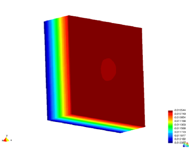
a) object 1	b) object 2
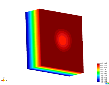
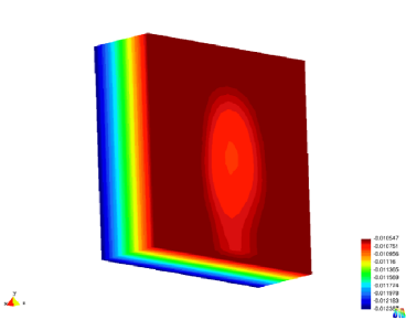
c) object 3	d) object 4
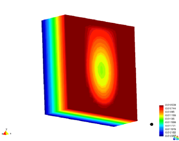
e) object 5	f) object 6

Figure 4: Behavior of functions $\psi_{n}(x)$ at $\partial\Omega$ for some objects of Table 1 at pseudo-frequency $s=9.2$.

8.2 Reconstructions

We collected experimental data for 11 targets presented in Table 1. Five targets were dielectrics, five were metallic ones, and one was a metal covered by a dielectric. We had total 7 blind cases: three dielectric, three metallic targets and one target was the above mixture of the metal and a dielectric. Three out of eleven targets were heterogeneous ones, all three were blind ones. Heterogeneous targets model explosive devices in which explosive materials are masked by dielectrics.

When proceeding with the algorithm of section 6.1, we first assign the Dirichlet boundary condition $\psi\left(\mathbf{x},s\right)$ at $\partial\Omega$ for the function $q\left(\mathbf{x},s\right)$ following (16), (18) and (19), in which case $\Gamma$ is as in (60). Next, we calculate functions $\psi_{n}\left(\mathbf{x}\right)$ as in (31). Figure 4 presents typical behavior of functions $\psi_{n}(x)$ at $\partial\Omega$ for some objects of Table 1. To have a better visualization, these figures are zoomed to $0.4\times 0.4$ square from the $1\times 1$ square.

Table 2 lists both computed $n^{\text{comp}}$ and directly measured refractive indices $n$ of dielectric targets for tests 1-3, see (58) for $n^{\text{comp}}$. This table also shows the measurement error in direct measurements of $n$. These measurements were performed by the classical oscilloscope method [10]. Table 3 lists computed appearing dielectric constants $\varepsilon_{r}^{\text{comp}}$ of metallic targets. Recall that $\varepsilon_{r}=n^{2}.$ We see from Table 2 that $\left(n^{\text{comp}}\right)^{2}<4.9$ for all dielectric targets. This is going along well with the Step 4 of the stopping criterion. On the other hand, in Table 3 $\varepsilon_{r}^{\text{comp}}>12$ for all metallic targets. Thus, our algorithm can confidently differentiate between dielectric and metallic targets.

Target number	1	2	5	8	10	Average error
blind/non-blind?	no	no	yes	yes	yes
Measured $n$, error	2.11, 19%	1.84, 18%	2.14, 28%	1.89, 30%	2.1, 26%	24%
$n^{\text{comp}}$ of Test 1, error	1.92, 10%	1.8, 2%	1.83, 17%	1.86, 2%	1.92, 9%	8%
$n^{\text{comp}}$ of Test 2, error	2.07, 2%	2.01, 10%	2.21, 3%	1.83, 3%	2.2, 5%	4.6%
$n^{\text{comp}}$ of Test 3, error	2.017, 5%	2.013, 9%	2.03, 5%	1.97, 4%	2.02, 4%	5%

Table 2: Computed $n^{\text{comp}}$ and directly measured refractive indices of dielectric targets together with both measurement and computational errors as well as the average error. Note that the average computing errors are at least three times less than the average error of direct measurements.

One can derive several important observations from Table 2. First, in all three tests and for all targets the computational error is significantly less than the error of direct measurements. Thus, the average computational error is significantly less than the average measurement error in all three tests. Second, computed refractive indices are within trust intervals in all cases. The accuracy of all three tests is about the same.

Table 3 provides information about computed appearing dielectric constants $\varepsilon_{r}^{\text{comp}}$ of metallic targets, see (5) and (58). Note that in Test 3 first four numbers $\varepsilon_{r}^{\text{comp}}=15$. This coincides with the upper bound in (64). On the other hand, $\varepsilon_{r}^{\text{comp}}=14<15$ for the target number 9. This is probably because target number 9 is a mixture of a metal and a dielectric. An important observation, which can be derived from Table 2, is that our algorithm confidently computes large inclusion/background contrasts exceeding 10:1. It is well known that optimization methods of conventional least squares residual functionals usually cannot image large contrasts.

Target number	3	4	6	7	9	11
blind/non-blind (yes/no)	no	no	yes	yes	yes	yes
$\varepsilon_{r}^{\text{comp}}$ of Test 1	14.4	15.0	15	13.6	13.6	13.1
$\varepsilon_{r}^{\text{comp}}$ of Test 2	15	15	15	14.1	14.1	15
$\varepsilon_{r}^{\text{comp}}$ of Test 3	15	15	15	15	14	14.06

Table 3: Computed appearing dielectric constants $\varepsilon_{r}^{\text{comp}}$ of metallic targets number 3,4,6,7,11 as well as of the target number 9 which is a metal covered by a dielectric.

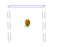
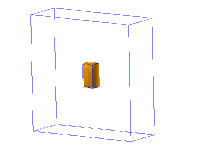
a) Test 1 (dielectric), object 1, first stage	b) Test 1 (dielectric), object 1, second stage
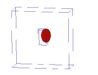
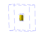
c) Test 1 (dielectric), object 5, first stage	d) Test 1 (dielectric), object 5, second stage

Figure 5: Computed images of targets numbers 1,5 of Table 1. Thin lines indicate correct shapes. To have better visualization we have zoomed images of Tests 1,2 from the domain $\Omega$ defined by (59) to the domain (63).

All targets, except of targets number 8, 9, 10, were homogeneous ones comprised from a single substance only. However, targets number 8-10 were inhomogeneous ones, see Table 1 for description of all targets. The target number 8 was a wooden doll which was empty inside. In the case of target number 9, a piece of a metal was inserted inside that doll. Thus, only the metal was imaged, because its reflection is much stronger than the wood. In the case of target number 10, sand was partly inserted inside that doll.

Figures 5 display 3-d images of some targets for Test 1 after the first and the second (postprocessing) stages described in section 7.2. Figures 6, 7 display 3-d images of targets 8,9,10 and 11 for all three tests.

Note that it is hard to estimate well the size of a target in the $z-$direction. Nevertheless, one can observe that rather good shapes and sizes of targets are computed in the case of prisms and cylinders, see Figure 5. As to the doll, neither of tests images shapes of targets 8-10 accurately. Still, the location of the doll  as well as its sizes in $x,y$ directions are well estimated, see Figures 6.

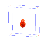
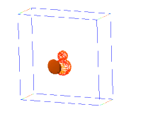
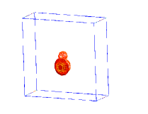
a) Test 1, object 8	b) Test 2, object 8	c) Test 3, object 8
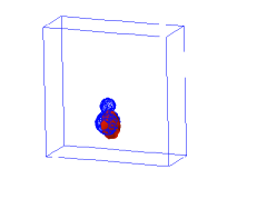
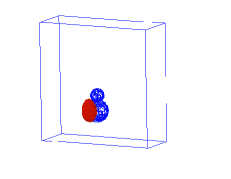
d) Test 1, object 9	e) Test 2, object 9	f) Test 3, object 9
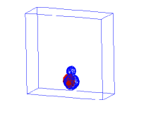
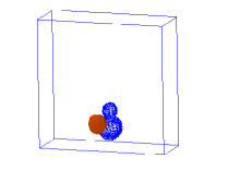
g) Test 1, object 10	h) Test 2, object 10	i) Test 3, object 10

Figure 6: Computed images of targets numbers 8,9,10 (see Table 1). Thin lines indicate correct shapes. To have better visualization we have zoomed images of Tests 1,2 from the domain $\Omega$ defined by (59) to the domain (63).

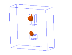
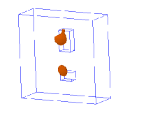
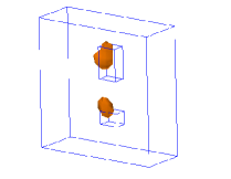
a) Test 1, object 11	b) Test 2, object 11	c) Test 3, object 11

Figure 7: Computed images of target number 11 of Table 1. Thin lines indicate correct shapes of two inclusions to be reconstructed. To have better visualization we have zoomed images of Tests 1,2 from the domain $\Omega$ defined by (59) to the domain (63).

9 Summary

We collected experimental backscattering time resolved data of electrical wave propagation and have applied the approximately globally convergent numerical method of [3] to these data. Results for four non-blind and seven blind cases show a good accuracy of reconstruction of refractive indices of dielectric targets and appearing dielectric constants of metallic targets. In the case of dielectrics, the average reconstruction error is at least three times less than the error of direct measurements. We confidently differentiate between metallic and dielectric targets. In particular, we have accurately computed maximal values of refractive indices/dielectric constants of three blind heterogeneous targets. These targets represent simplified models of improvised explosive devices IEDs, which are heterogeneous ones.

Locations of targets and their sizes in $x,y$ directions are accurately reconstructed. The most difficult cases of sizes in the $z-$direction (depth) are well reconstructed in some cases. In addition, shapes of some targets are well reconstructed in some cases. We believe that a follow up application of the locally convergent adaptivity technique might improve reconstructions of shapes of targets. The adaptivity takes the solution obtained by the approximately globally convergent method as the starting point for the minimization of the Tikhonov functional on a sequence of adaptively refined meshes. A significant refinement via the adaptivity was demonstrated in section 5.9 of [3] for the case of transmitted experimental data, see Figures 5.13 and 5.16 in [3].

Acknowledgments

This research was supported by US Army Research Laboratory and US Army Research Office grants W911NF-11-1-0325 and W911NF-11-1-0399, the Swedish Research Council, the Swedish Foundation for Strategic Research (SSF) through the Gothenburg Mathematical Modelling Centre (GMMC) and by the Swedish Institute, Visby Program. The authors are grateful to Mr. Steven Kitchin for his excellent work on data collection.

References

- [1] A.B. Bakushinsky and M.Yu. Kokurin, Iterative Methods for Approximate Solutions of Inverse Problems, Springer, New York, 2004.
- [2] L. Beilina, K. Samuelsson and K. Ahlander, Efficiency of a hybrid method for the wave equation. In International Conference on Finite Element Methods, Gakuto International Series Mathematical Sciences and Applications, Gakkotosho CO., LTD, 2001.
- [3] L. Beilina and M.V. Klibanov, Approximate Global Convergence and Adaptivity for Coefficient Inverse Problems, Springer, New York, 2012.
- [4] L. Beilina and M.V. Klibanov, A new approximate mathematical model for global convergence for a coefficient inverse problem with backscattering data, J. Inverse and Ill-Posed Problems, 20, 513-565, 2012.
- [5] L. Beilina, Energy estimates and numerical verification of the stabilized domain decomposition finite element/finite difference approach for the Maxwell’s system in time domain, Central European Journal of Mathematics, 11, 702-733, 2013.
- [6] A.L. Bukhgeim and M.V. Klibanov, Uniqueness in the large of a class of multidimensional inverse problems, Soviet Math. Doklady, 17, 244-247, 1981.
- [7] G. Chavent, Nonlinear Least Squares for Inverse Problems. Theoretical Foundations and Step-By-Step Guide for Applications, Springer, New York, 2009.
- [8] H.W. Engl, M. Hanke and A. Neubauer, Regularization of Inverse Problems, Kluwer Academic Publishers, Boston, 2000.
- [9] B. Engquist and A. Majda, Absorbing boundary conditions for the numerical simulation of waves, Math. Comp., 31, 629-651, 1977.
- [10] H.H. Gerrish, W.E.Jr. Dugger and R.M. Robert, Electricity and Electronics, Goodheart-Wilcox Co. Inc., Merseyside, UK, 2004.
- [11] V. Isakov, Inverse obstacle problems, Inverse Problems, 25, 123002, 2009.
- [12] C. Johnson, Numerical Solution of Partial Differential Equations by the Finite Element Method, Cambridge University Press, Cambridge, 1987.
- [13] A.V. Kuzhuget, L. Beilina, M.V. Klibanov, A. Sullivan, L. Nguyen and M.A. Fiddy, Blind experimental data collected in the field and an approximately globally convergent inverse algorithm, Inverse Problems, 28, 095007, 2012.
- [14] O.A. Ladyzhenskaya and N.N. Uralceva, Linear and Quasilinear Elliptic Equations, Academic Press, New York, 1969.
- [15] N. T. Thành, L. Beilina, M. V. Klibanov, and M. A. Fiddy. Reconstruction of the refractive index from experimental backscattering data using a globally convergent inverse method, Preprint, arXiv:1306.3150 [math-ph], 2013.
- [16] M. Soumekh, Syntetic Aperture Radar Signal Processing, Willey&Son, New York, 1999.
- [17] C.R. Vogel, Computational Methods for Inverse Problems, SIAM Publications, Philadelphia, 2002.
- [18] WavES, the software package, http://www.waves24.com