On the non-equivalence of perfectly matched layers and exterior complex scaling

Abstract

The perfectly matched layers (PML) and exterior complex scaling (ECS) methods for absorbing boundary conditions are analyzed using spectral decomposition. Both methods are derived through analytical continuations from unitary to contractive transformations. We find that the methods are mathematically and numerically distinct: ECS is complex stretching that rotates the operator’s spectrum into the complex plane, whereas PML is a complex gauge transform which shifts the spectrum. Consequently, the schemes differ in their time-stability. Numerical examples are given.

1 Introduction

An important problem in numerical simulations of time dependent equations is the need to restrict infinite domains to finite computational domains for purposes of approximation. A simple cutoff of the domain by trivial boundary conditions (e.g. imposing zero Dirichlet boundary conditions, or periodic continuation) leads to errors at the boundary of the (artificial) domain of simulation as soon as the solution is not small enough anymore near the boundary. Much work has been dedicated to the question of how to either remove these errors totally or to sufficiently suppress them. A popular method to prescribe artificial absorbing boundary conditions is the perfectly matched layer method (PML). A slightly older method uses a very similar, but nonetheless distinct approach called exterior complex scaling (ECS). This method has mainly been applied to dispersive problems, like, e.g., the Schrödinger equation.

The ECS was proposed by B. Simon [1] as an extension of the complex scaling method first established by Balslev and Combes [2] for Schrödinger operators. The PML approach initially was introduced by Berenger [3] for application to Maxwell equations or wave equations, but later also was applied to Schrödinger type equations.

There exist several other methods to treat the domain cutoff problem, for example transparent boundary conditions, complex absorbing potentials (optical potentials), or time dependent phase space filters, which are not subject of this work. An overview of most of these methods can be found in [4].

A large body of mathematical physics literature exists on ECS (many references can be found, e.g., in [5]). Early computational applications were for the computation of decaying states in quantum chemistry (see, e.g., [6, 7]). In [8] the numerical realization of ECS was improved by using infinite range basis elements in the boundary region and thus considerably increasing the efficiency of the method.

PML was applied to Maxwell equations by Chew and Wheedon, e.g., in [9]. A recent study on PML for general hyperbolic problems with (algorithmic) stability is found in [10]. We mention also a work by Lions et.al. on a stabilized PML method [11]. Concerning the application of PML to the Schrödinger case, the first study was [12]. In this work, the PML method when applied to the Schrödinger equation was actually modified to be conceptually equivalent to the ECS method. As far as we are aware, the same is true for other works on PML for Schrödinger type equations. Recent contributions to this subject are [13, 14, 15]. Loh et.al. studied the failure of the PML method for wave guides with backward wave structures [16].

ECS and PML share the general idea of using analytic continuation of the equation outside a finite spatial domain. However, in their respective original formulations, the approaches differ qualitatively. This is already evident from the absence of ECS methods for wave equations and from the comparatively poor performance of PML for the TDSE. In the present work we analyze both methods in a common analytic approach using spectral analysis. This clearly exposes the differences between them and explains their different stability behavior for Schrödinger-like and wave-like equations, respectively. The distinct spectral characteristics have immediate bearings on the numerical implementation. In brief, ECS rotates the continuous spectrum into the complex plane, while PML shifts the spectrum. In the spatial domain this corresponds to stretching of the coordinates and a complex gauge transform, respectively. PML is applicable for operators like $-i\partial_{x}$ whose spectrum covers all ${I\!\!R}$, while ECS works well on Schrödinger operators with continuous spectrum on ${I\!\!R}_{+}$. We could not formulate a version of ECS that would work with $-i\partial_{x}$, while we could obtain highly accurate results for the TDSE with both, ECS and PML. With the Schrödinger equation, we found PML to be less accurate than ECS, where full computational precision could be reached.

In the following, after specifying the wave and Schrödinger equations, we present in detail the spectral analysis of ECS. The analogous discussion is presented for PML, before we give numerical examples. We conclude with pointing to the potential of the approach for designing absorbing boundary methods for general linear wave equations.

2 Model equations

The goal is to provide absorbing boundaries for time-dependent evolution equations. The class of problems usually treated by these methods includes, both, dispersive and hyperbolic equations, and in general problems which allow wave-type solutions. For the purposes of this discussion, we consider the time-dependent Schrödinger equation and a wave equation typical model problems from this class, which can both be formulated as a first order propagation equation

(2.1) $$i\frac{\partial}{\partial t}\phi=D\phi$$

with a self-adjoint operator $D$ acting on the space variable.

The scalar wave equation in reads

(2.2) $$i\frac{\partial}{\partial t}\phi=-i\nabla\phi.$$

The time-dependent Schrödinger equations reads

$$i\frac{\partial}{\partial t}\phi[t](x)=[-\frac{1}{2}\Delta+V(x)]\phi[t](x).$$

where $V(x)$ is a potential term. ECS is rigorously applicable for non-zero $V(x)$, but for the sake of simplicity in the present discussion, we restrict ourselves to $V(x)\equiv 0$.

3 Spectral analysis of ECS

When solving Eq. (2.1) one is usually interested in the solution $\phi[t](x)$ only on a finite domain $x\in F\subset{I\!\!R}$. Outside $F$ the solution can be damped or otherwise removed. A basic assumption of ECS, and equally of PML, is that asymptotically the solution takes the form

$$\phi[t](x)\stackrel{{\scriptstyle|x|\to\infty}}{{\sim}}\int_{0}^{\infty}d\omega\tilde{\psi}(\omega)\exp[i|k(\omega)||x|],$$

i.e. it has outgoing asymptotics. The functional dependence of the wave vector $k(\omega)$ on the frequency $\omega$ determines the system’s dispersion. The idea is to convert the unlimited spatial extension of an outgoing solution to exponentially decaying form by continuing it into the positive complex plane for $x\not\in F$. The numerical approximation of the exponentially decaying solution requires much smaller grids than the full solution. Let us label the analytically continued solution by a complex number $\eta$. For the new equation with exponentially decaying asymptotics

(3.1) $$i\frac{\partial}{\partial t}\psi_{\eta}[t](x)=D_{\eta}\psi_{\eta}[t](x),$$

one wants the following property to hold:

(3.2) $$\phi[t](x)=\psi_{\eta}[t](x)\quad{\rm for}\quad x\in F,\forall t.$$

For this, one constructs the transformation such that it is unitary for real values of $\eta$ and (3.2) holds. For complex $\eta$ one can obtain an asymptotically decaying solution and use analyticity arguments to show that (3.2) holds.

A second requirement crucial for numerical use of (3.1) is stability: for propagation towards positive times, the spectrum of the discrete representation of $D_{\eta}$ must be in the lower half complex plane. Spectral components with positive imaginary parts will lead to exponential growth of the $L^{2}$-norm of $\psi_{\eta}$ and to numerical breakdown of the time-propagation, irrespective of the particular propagation scheme used.

The necessary spectral properties under these transformations have been proven for a wide class of Schrödinger operators that includes few-body Coulomb systems and a large class of particles interacting by short range potentials (for a review see, e.g.,[17]). For those “dilation analytic” Schrödinger operators, $D_{\eta}$ can be defined as an operator on the position space $\mathcal{H}_{x}=L^{2}(dx,{I\!\!R})$ with spectrum in the lower complex half-plane. Note that the numerical scheme must be set up such that also the discretized operators have no spectrum in the upper complex plane.

Earlier applications of complex scaling to time-dependent problems [18, 19] were using $F=\emptyset$, i.e. no directly usable information on $\phi[t](x)$ was obtained and only matrix elements could be computed using analytical continuation. In recent literature, applications of ECS were reported, where, however, severe numerical shortcomings were observed [20, 21]. The difficulties were overcome in “infinite range ECS” [8], where results of machine precision accuracy were obtained employing as few as 10 grid points for absorption. The underlying mathematical rational is laid out now.

Considering that the operator $D$ is self-adjoint on $L^{2}(dx,{I\!\!R})$ with domain $\mathcal{D}(D)$ and spectrum $\sigma(D)\subset{I\!\!R}$ we can spectrally decompose the solutions as

$$\tilde{\psi}[t](\omega)=(W^{-1}\psi[t])(\omega)=\int dx\overline{w(x,\omega)}\psi[t](x),\quad\omega\in\sigma(D).$$

The integral kernel of the unitary map $W:\mathcal{H}_{\omega}:=L^{2}\left(d\mu(\omega),\sigma(D)\right)\to\mathcal{H}_{x}:=L^{2}(dx,{I\!\!R})$ defines the spectral eigenfunctions $w(x,\omega)$. We can write

(3.3) $$(D\psi)(x) = \int_{\sigma(D)}d\mu(\omega)w(x,\omega)\omega\int dx^{\prime}\overline{w(x,\omega)}\psi(x^{\prime})$$

(3.4) $$= \int_{\sigma(D)}d\omega\rho(\omega)w(x,\omega)\omega\int dx^{\prime}\overline{w(x,\omega)}\psi(x^{\prime}).$$

Here $d\mu(\omega)$ denotes the spectral measure. In the last line we have, for notational simplicity, assumed that $D$ has a purely absolutely continuous spectrum, which allows us to extract the “density of states” $\rho(\omega)\geq 0$ as an absolutely continuous function. For now, we disregard a possible multiplicity of the spectrum. The spectral representation of $D$ is briefly written as

$$D=W\hat{\omega}W^{-1},$$

where $\hat{\omega}$ denotes multiplication by $\omega$ in $\mathcal{H}_{\omega}$.

To arrive at the scaled equation (3.1) one takes the following steps:

• Introduce unitary scaling $U_{\lambda}$ that leaves the solutions invariant on $F$ for a range of real values of $\lambda$. With this, define a self-adjoint (real) scaled operator $D_{\lambda}:=U_{\lambda}DU_{\lambda}^{-1}$. Ideally, show analyticity properties of the $D_{\lambda}$ w.r.t. $\lambda$.

• Solve Eq. (3.1) in the spectral domain and show that $\psi_{\lambda}[t](x)$ is an analytic function of $\lambda$.

• Analytically continue to complex values $\eta=\lambda+i\theta$ and conclude that $\psi_{\eta}[t](x),x\in F$ does not depend on $\eta$.

• Show that $\psi_{\eta}[t](x)$ does nowhere grow exponentially in time, i.e. the analytically continued operator $D_{\eta}$ has no eigenvalues in the upper complex half-plane.

3.1 Real scaling by $U_{\lambda}$

Exterior real scaling is the transformation

(3.5) $$(U_{\lambda}\psi)(x)=e^{\lambda\Theta_{F}(|x|)/2}\psi(z_{\lambda}(x)),\quad z_{\lambda}(x):=\frac{x}{|x|}\int_{0}^{|x|}dre^{\lambda\Theta(r)}$$

with

$$\Theta_{F}(|x|)=0\quad{\rm for}\quad x\in F,\quad\Theta_{F}(|x|)>0\quad{\rm else}.$$

$U_{\lambda}$ is manifestly unitary for all $\lambda\in{I\!\!R}$. The exact choice of $\Theta$ is unessential for the present discussion but impacts on discretization. Note that $\Theta$ can be discontinuous. We will use the discontinuous function $\Theta(|x|)=1$ for $x\not\in F$, which leads to analytically simple and numerically efficient scaling.

With discontinuous scaling, one needs to worry about the correct definition of derivatives. It is easy to show that on functions $\chi\in\mathcal{D}(D_{\lambda})$ with the scaled domain $\mathcal{D}(D_{\lambda})=U_{\lambda}\mathcal{D}(D)$, $D_{\lambda}$ is self-adjoint. It has a spectral representation

(3.6) $$D_{\lambda} = W_{\lambda}\hat{\omega}W_{\lambda}^{-1}$$

$$= \int_{\sigma(D_{\lambda})}d\omega\rho_{\lambda}(\omega)w_{\lambda}(x,\omega)\omega\int dx^{\prime}\overline{w_{\lambda}(x,\omega)}\psi(x^{\prime}),$$

with the scaled spectral eigenfunctions

(3.7) $$w_{\lambda}(x,\omega):=(U_{\lambda}w)(x,\omega).$$

Unitarity of $U_{\lambda}$ ensures that $\sigma(D_{\lambda})=\sigma(D)$. Note, however, that functions $\chi_{\lambda}\in\mathcal{D}(D_{\lambda})$ and also their derivatives are discontinuous at the borders $x_{0}\in\partial F$ of $F$ in the form

(3.8) $$\chi_{\lambda}(x_{0}+0) = e^{\lambda/2}\chi_{\lambda}(x_{0}-0)$$

(3.9) $$\chi^{\prime}_{\lambda}(x_{0}+0) = e^{3\lambda/2}\chi^{\prime}_{\lambda}(x_{0}-0).$$

The functions $w_{\lambda}(x,\omega)=(U_{\lambda}w)(x,\omega)$ are orthonormal in the sense

$$\int_{I\!\!R}dx\,\overline{w_{\lambda}(x,\omega)}w_{\lambda}(x,\omega^{\prime})=\rho(\omega)\delta(\omega-\omega^{\prime}).$$

The spectral representation is defined by a unitary transformation to an $L^{2}$-space of functions on the spectrum of the operator, where the operator appears as multiplication by $\omega$. Therefore the spectral density $\rho_{\lambda}(\omega)\neq\rho(\omega)$ must be considered as $\lambda$-dependent, when we use the $w_{\lambda}(x,\omega)$ defined in (3.7). The spectral resolution of identity is

(3.10) $$\chi(x)=\int_{\sigma(D)}d\omega\rho_{\lambda}(\omega)w_{\lambda}(x,\omega)\int_{I\!\!R}dx^{\prime}\overline{w_{\lambda}(x^{\prime},\omega)}\chi(x^{\prime}).$$

Let us illustrate the $\lambda$-dependence of $\rho_{\lambda}$ in the simple case of global scaling $F=\emptyset$ for the wave-equation with $D=-i\partial_{x}$. For a scaled spectral eigenfunction it acts as

$$-i\partial_{x}U_{\lambda}\frac{1}{\sqrt{2\pi}}e^{i\omega x}=-i\partial_{x}\frac{1}{\sqrt{2\pi}}e^{i\omega e^{\lambda}x}=\frac{e^{\lambda}}{\sqrt{2\pi}}\omega e^{i\omega x}.$$

We see that the set of spectral eigenfunctions and overall spectrum remain the same, but the association of a given $\omega$ with individual spectral functions $w_{\lambda}(x,\omega)$ changes, in this case by the factor $e^{\lambda}$. This factor must be compensated by a change in the density of states. For this particular example $\rho_{\lambda}(\omega)=e^{-\lambda}$. For $F=\emptyset$ we have $\mathcal{D}(D_{\lambda})=\mathcal{D}(D)$ and we may just as well re-define the integration variable $\omega\to\omega^{\prime}=e^{\lambda}\omega$ and find $U_{\lambda}\partial_{x}U_{\lambda}^{-1}=e^{-\lambda}\partial_{x}$, a rather obvious result in this case.

As it turns out, the modification of the spectral density for the operators $-i\partial_{x}$ and $-\partial_{x}^{2}$ depends only on the asymptotic behavior of the solution and it is independent of any finite $F$. This also holds when adding a “dilation analytic” potential to the differential operators. In fact, the $D_{\lambda}$ can be considered as an operator-valued analytic function. We refer the reader to [17] for a detailed discussion. Accepting this assertion, we can continue our formal discussion in the spectral domain.

For solving (3.1) we go into the spectral representation by applying the resolution of identity (3.10)

(3.11) $$i\frac{\partial}{\partial t}\tilde{\psi}_{\lambda}[t](\omega)=\rho_{\lambda}(\omega)\omega\tilde{\psi}_{\lambda}[t](\omega).$$

In $\mathcal{H}_{\omega}$ the solution is

(3.12) $$\tilde{\psi}_{\lambda}[t](\omega)=e^{-i\rho_{\lambda}(\omega)\omega t}\tilde{\psi}_{\lambda}[0](\omega),\quad\tilde{\psi}_{\lambda}[t](\omega)=(W_{\lambda}^{-1}\psi_{\lambda}[t])(\omega)$$

and in $\mathcal{H}_{x}$ it is

(3.13) $$\psi_{\lambda}[t]=\int d\omega\rho_{\lambda}(\omega)w_{\lambda}(x,\omega)e^{-i\rho_{\lambda}(\omega)\omega t}\tilde{\psi}_{\lambda}[0](\omega).$$

For any unitary $U_{\lambda}$, it trivially holds that

$$\psi_{\lambda}[t](x)=U_{\lambda}\psi[t](x).$$

Equality is to be understood in the $L^{2}$-sense on sets of measure $>0$, not point-wise. As our exterior scaling $U_{\lambda}$ changes functions only outside $F$ we have

(3.14) $$\psi_{\lambda}[t](x)=\psi[t](x)\quad{\rm for}\quad x\in F,\forall\,t.$$

3.2 Analytic continuation

We analytically continue the integrand on the r.h.s. of Eq. (3.13) to complex values of $\lambda$. If the initial state $\psi[0](x)$ has its support in $F$, its spectral components are independent of $\lambda$

$$\tilde{\psi}_{\lambda}[0](\omega)=\int_{F}dx\overline{w_{\lambda}(x,\omega)}\psi[0](x)=\int_{F}dx\overline{w(x,\omega)}\psi[0](x)=\tilde{\psi}[0](\omega).$$

$\rho_{\lambda}(\omega)$ is $e^{-\lambda}$ and $e^{-2\lambda}$ for $D$ asymptotically $\sim-i\partial_{x}$ and $\sim-\partial_{x}^{2}$, respectively. Finally, the spectral eigenfunctions are

$$w_{\lambda}(x,\omega)\sim\exp[ik(\omega)e^{\lambda}\Theta(x)x],$$

with $k(\omega)=\omega$ for $-i\partial_{x}$ and $k(\omega)=\pm\sqrt{\omega}$ for $-\partial_{x}^{2}$.

The spectral representation (3.13) then reads, after analytical continuation $\lambda\to i\theta$ ($\theta\in{I\!\!R}$)

(3.15) $$\psi_{\theta}[t](x)=\int d\omega e^{-in\theta}w_{\theta}(x,\omega)e^{-i\cos(n\theta)\omega t}e^{-\sin(n\theta)\omega t}\tilde{\psi}[0](\omega).$$

with $n=1,2$ for asymptotic behavior $\sim(-i\partial_{x})^{n}$.

The complex scaled solution $\psi_{\theta}[t](x)$ is analytic in $\theta$, as it is an integral of analytic functions. From analyticity and independence of $\psi_{\lambda}[t](x)$ for real $\lambda$ it follows that the solution agrees with the unscaled solution on $F$, i.e. Eq. (3.2) is satisfied.

Finally we examine the spatial and temporal behavior of the scaled solution. If in the unscaled solution $\psi_{\theta=0}[t]$ has outgoing behavior, then, by analyticity, the scaled solution $\psi_{\theta>0}[t]$ at fixed time $[t]$ decays exponentially with $|x|$. The operator $-\partial_{x}^{2}$ has strictly positive spectral values $\omega$ and therefore, for positive $\sin(2\theta)$, the solution is non-growing in time.

However, we see that for $-i\partial_{x}$ the solution will contain components that grow in time: its spectrum covers positive as well as negative $\omega$ and therefore $\sin(n\theta)\omega$ cannot be positive over the complete spectrum for constant $\theta$. This cannot be controlled in ECS in the present form. A restriction of $\tilde{\psi}[0](\omega)$ to one spectral half-axis is not desirable, as it excludes initial states that are spatially confined to $F$. Even more importantly, in a computational scheme formulated in $\mathcal{H}_{x}$ rather that $\mathcal{H}_{\omega}$, numerical noise will always generate components throughout the spectrum, which cause fatal numerical instability. Below we discuss, how PML avoids this problem by a different analytical continuation scheme.

In principle, similar reasoning as for temporal instability might be used for the spatial buildup of undesired ingoing components, i.e. for the spatial growth towards grid boundaries. However, in this case the spatial discretization itself, e.g. by using a square-integrable basis set, suppresses any spatially growing components. The fact that we are allowed to simply suppress ingoing components must be derived from a priori knowledge of our solution. This is usually either exactly known or a physically motivated assumption.

Also, note that the suppression of ingoing waves is only asymptotic. From any domain outside $F$, wave amplitude can return into $F$. In fact, clear numerical evidence was found in [8] that this happens without compromising the solution on $F$. Absorption in the sense of loss of information is only caused by finite numerical accuracy in representing the exponential tail of the solution.

4 Spectral analysis of PML

PML is often introduced in the same way as ECS. Then, in a final step, each spectral function $w(x,\omega)$ is scaled separately by an $\omega$-dependent factor. The procedure is motivated as to create a uniform exponential decay for all wave vectors, rather than the $k(\omega)$-dependent damping of ECS. For scaling of $-i\partial_{x}$ one replaces in (3.5) $e^{\lambda\Theta_{F}/2}\to 1+\lambda/\omega\Theta_{F}$. A space-dependent spectral shift by $\lambda$ results:

$$U_{\lambda}^{(PML)}e^{i\omega x}=e^{i\omega(1+\lambda/\omega\Theta_{F}(x))x}=e^{i(\omega+\lambda\Theta_{F}(x))x}.$$

Indeed, the intended effect is achieved: for $\lambda=i\theta$ all spectral functions decay equally as $e^{-\theta x}$. Depending on the numerical implementation, this may or may not facilitate numerical approximation. Its crucial effect, however, is to make the scheme temporally stable by the $\omega$-dependent sign change: negative frequency components are stretched with the opposite sign of the positive frequency components. When continuing the solution into the complex plane, both, positive and negative frequency parts of the spectrum become exponentially damped simultaneously. For functions $\phi\in\mathcal{H}_{x}$, $U_{\lambda}^{(PML)}$ is a (local) gauge transform:

$$(U_{\lambda}^{(PML)}\phi)(x)=e^{i\lambda\Theta_{F}(x)x}\phi(x).$$

Obviously, $U_{\lambda}^{(PML)}$ is unitary for $\lambda\in{I\!\!R}$. Let us use $D=-i\partial_{x}$. On functions $\chi\in\mathcal{D}(D_{\lambda}^{(PML)})=U_{\lambda}^{(PML)}\mathcal{D}(D)$, the PML derivative is

$$D_{\lambda}^{(PML)}\chi=e^{i\lambda\Theta_{f}(x)}De^{-i\lambda\Theta_{f}(x)}\chi=[D-\lambda\Theta_{f}(x)]\chi.$$

By choosing $\chi\in\mathcal{D}(D_{\lambda})$, we have made sure not to get $\delta$-like contributions at $\partial F$.

Now we can use the same general reasoning as in the case of exterior complex scaling to conjecture that on $F$ the solutions of

$$i\frac{\partial}{\partial t}\psi_{\lambda}[t]=D_{\lambda}^{(PML)}\psi_{\lambda}[t]=[D-\lambda\Theta_{f}(x)]\psi_{\lambda}[t]$$

agree with $\phi[t](x)$, Eq. (3.2). Invoking analyticity arguments, this can be extended to complex values $\lambda\to i\theta$, for which the solutions $\psi_{i\theta}[t]$ will be exponentially decaying outside $F$. As the absolutely continuous spectrum is determined by the asymptotic behavior, all frequencies $\omega$ of the time-evolution experience a uniform spectral shift to into the lower half plane to $\omega-i\theta$.

4.1 Frequency dependent PML for the Schrödinger equation

As mentioned in the introduction, a large amount of literature exists on the topic of scaling-based absorbing layers for time dependent Schrödinger equations. The first work on the subject was done by Collino [12], where the TDSE appears in the context of modeling of waves as a paraxial approximation of a higher dimensional equation. The frequency used in construction of the PML is actually a carrier frequency in the superseding high-dimensional model, which in the paraxial TDSE equation appears only as a constant. So for the TDSE, the PML used by Collino did not use frequency-dependent rescaling and was actually equivalent to the ECS method. (However the rescaling was not formulated to be unitary, consisting instead only of a coordinate transform.) Other authors on the subject are Levy [22], Farrell and Leonhardt [23] and Zheng [13], who all followed the same approach using a method equivalent to ECS ($\omega$-independent rescaling). In [24], the coupled mode equations are studied, which are a combination of the two model cases considered here, and combine hyperbolic operators in one space direction and a Schrödinger-like operator in the perpendicular direction. The PML method for these equations is $\omega$-dependent. In [14], a slightly generalized TDSE is studied which includes mixed derivatives of second order. $\omega$-independent rescaling is used. The recent work of Nissen et.al. [15] uses a rescaling of both variable and wave function which is not unitary, but instead is used to obtain a formulation of the scaled operator which avoids first order derivative terms. Here, again, rescaling is not depending on $\omega$, which makes the method of ECS type.

We will now investigate the behavior of $\omega$-dependent PML for the TDSE. A local gauge transform $U_{\lambda}^{(PML)}$ generates

$$D_{\lambda}=(-\partial_{x}^{2})_{\lambda}=-\partial_{x}^{2}-2i\lambda\Theta_{F}(x)\partial_{x}+\Theta_{F}(x)\lambda^{2}$$

with the spectral values

$$\omega\to(\pm\sqrt{\omega}+\lambda)^{2}=\omega\pm 2\sqrt{\omega}\lambda+\lambda^{2}.$$

Analytic continuation to complex values $\lambda\to\eta=\lambda e^{i\alpha}$ invariably introduces positive as well as negative imaginary parts in the spectrum. However, we may numerically suppress ingoing waves $k(\omega)x<0$: by making the gauge transform dependent on the sign of $x$

$$\Theta(x):=\left\{\begin{array}[]{rl}0&{\rm for}\quad x\in F\\ 1&{\rm for}\quad 0<x\not\in F\\ -1&{\rm for}\quad 0>x\not\in F.\end{array}\right.$$

With $0<\lambda$ and complex phase $0<\alpha<\pi/2$, all outgoing spectral components decay exponentially in space. In addition, they are associated with spectral values in the lower complex half plane and decay exponentially in time. Ingoing components, which would be exponentially growing in space and time, are assumed not to occur in the solution. They are excluded from the discrete problem by choosing square-integrable representation. If the complex argument is chosen at $\alpha=\pi/2$, the transformation maps $\omega=0\to-\lambda^{2}$, back to the negative real axis, and time-decay of small-$\omega$ components becomes inefficient. Indeed, with complex arguments $\alpha$ approaching $\pi/2$, the PML for the TDSE starts to break down (see numerical examples below).

We cannot, at this point, provide mathematical proof for this formal reasoning. The theory of dilation-analytic operators is inapplicable here. However, this does not mean that the absorption scheme fails. Even more severe mathematical questions arise in ECS for the Stark-effect where a potential of the form $x\mathcal{E}$ is added to the Hamiltonian. Likewise, adding time-dependent dipole interactions $iA(t)\partial_{x}$ as in [8] extends the spectrum to all ${I\!\!R}$. Yet, in both cases, ECS delivers verifiably accurate results (see, e.g., [19, 25]).

5 Numerical evidence

Without further investigating the mathematical arguments, we now show that numerical experiments confirm the above formal expectations. For a detailed numerical study of ECS we refer to a series of recent publications on absorption by ECS in one and three dimensions [8, 26, 27]. ECS was found to provide perfect (machine precision) absorption for 1d and 3d problems, even when the Schrödinger operator contains an explicitly time-dependent part.

All numerical calculations are performed using a high order finite element spatial discretization. As the scheme relies on analyticity, when using our discontinuous $\Theta_{F}$, it is important to correctly implement the discontinuity at $\partial F$. One might think of starting from basis functions $\phi_{i}\in\mathcal{D}(D)$ and use $\phi_{i}^{(\lambda)}(x)=(U_{\lambda}\phi_{i})(x)$. However, in that case, for real $\lambda$ all matrix elements of the transformed equation would be trivially identical to the matrix elements of the original equation with the untransformed basis and this property would carry over to complex $\eta$. The correct strategy is to discretize the transformed domain $\mathcal{D}(D_{\eta})$, where we can take advantage of the exponentially damped character of the solution. One possibility to build the discontinuity (3.8) into the basis is by using $\chi_{i}^{(\lambda)}(x)=e^{-\lambda/2\Theta_{F}(x)}\chi_{i}(x)$, where the $\chi_{i}$ are everywhere differentiably continuous. The discontinuity of the first derivative does not need to be imposed, if we compute matrix elements by partial integration as

$$\left(\widehat{D}_{\lambda}\right)_{ij}:=\langle\chi_{i}^{(\lambda)}|\left(-\partial_{x}^{2}\right)_{\lambda}|\chi_{j}^{(\lambda)}\rangle=\int_{F}dx\overline{\chi^{\prime}_{i}(x)}\chi^{\prime}_{j}(x)+e^{-\lambda}\int_{{I\!\!R}\backslash F}\!\!\!dx\overline{\chi^{\prime}_{i}(x)}\chi^{\prime}_{j}(x).$$

The $e^{\lambda}$ from the discontinuity partially cancels with $e^{-2\lambda}$ from the scaled second derivative leaving the overall factor $e^{-\lambda}$ in front of the second summand. The $\lambda$-dependence of the basis here also affects the overlap matrix

$$\left(\widehat{S}_{\lambda}\right)_{ij}=\int_{F}dx\,\overline{\chi_{i}(x)}\chi_{j}(x)+e^{\lambda}\int_{{I\!\!R}\backslash F}dx\,\overline{\chi_{i}(x)}\chi_{j}(x).$$

Continuation $\lambda\to\eta\in{I\!\!\!\!C}$ leads to a non-hermitian overlap matrix. For real $\chi_{i}$, $\widehat{S}_{\eta}$ is complex symmetric: $\left(\widehat{S}_{\eta}\right)_{ij}=\left(\widehat{S}_{\eta}\right)_{ji}$.

In PML, the basis for real $\lambda$ is multiplied by a $x$-dependent phase, which leaves the overlap matrix elements unaffected for all real $\lambda$, and no complex continuation of the overlap matrix is needed: $\widehat{S}^{(PML)}_{\eta}\equiv\widehat{S}$. This is a relevant technical difference between ECS and PML.

One finally solves the discretized system

$$i\frac{\partial}{\partial t}{\vec{c}}=\widehat{S}_{\eta}^{-1}\widehat{D}_{\eta}{\vec{c}}$$

by some standard ODE solver. In the present work we chose a step-size controlled classical 4th order Runge-Kutta.

5.1 Spatial discretization, initial state, propagation time

No effort was made to optimize the spatial discretization for the individual methods. Rather, we choose a very exhaustive basis to numerically support the claims on analyticity and stability made above. For all calculations we chose a basis of standard polynomial finite elements on $F$. Outside, we use a combination of polynomial finite elements with polynomials times a decaying exponential $Q_{n}(x)\exp(\mp\alpha x)$ for the first and last element with $x\to\mp\infty$, respectively. A detailed description of this basis, which defines the “infinite range”ECS method, can be found in [8]. Here we used $\alpha=6$ and polynomial orders $n=20$ and $N\times N$ sizes of $N\approx 360\sim 560$ for $\widehat{S}_{\eta}$ and $\widehat{D}_{\eta}$ matrices. Clearly, with some optimization, significantly smaller bases can be used. However, as we wanted to present results independent of discretization issues, this significantly over-saturated basis was used.

Our initial state is

(5.1) $$\psi[0](x)=\left\{\begin{array}[]{cl}\cos^{2}(\pi x/4)e^{ix}&{\rm for}\quad x\in[-2,2]\\ 0&{\rm else.}\end{array}\right.$$

We choose $F=[-2.5,2.5]$ and propagate until $t=2.5$. At that time, the center of the initial distribution falls onto the right hand boundary $\partial F=2.5$. The accuracy of $\psi_{\eta}[t]$ is studied by comparison with a solution $\phi_{\eta}[t]$ on an extended domain $F_{\phi}=[-5,5]$.

5.2 The wave equation

Figure 1: (color online) Relative error $E(x)$ of $\psi_{\eta}[t]$ at time $t=2.5$ for the wave equation computed with PML absorption. The error is defined in Eq. (5.2).

Figure 1 shows our best PML solutions for the wave equation 2.2 with initial state (5.1) $\psi_{\eta}^{(PML)}[t]$ and $\phi_{\eta}^{(PML)}[t]$ at $t=2.5$. In the calculations, we used $\eta^{(PML)}=5i$, but the results are independent of the exact choice of $\eta$. The relative error

(5.2) $$E(x)=\frac{|\psi_{\eta}^{(PML)}[t](x)-\phi_{\eta}^{(PML)}[t](x)|}{|\psi_{\eta}^{(PML)}[t](x)+\phi_{\eta}^{(PML)}[t](x)|}$$

nowhere on $[0.5,2.5]$ exceeds $10^{-5}$ and near the edge it is $\sim 10^{-7}$. The remaining error is largely do to numerical loss in our propagation scheme.

Not surprisingly, PML works as expected for the simple 1d wave equation. For the reasons discussed above, the wave equation diverges when using ECS and no numerical results were obtained.

5.3 The TDSE

Figure 2 shows the best achieved ECS and PML solutions of the TDSE and their relative errors. We used scaling parameters $\eta^{(ECS)}=e^{i\theta}=e^{i/2}$ and $\eta^{(PML)}=5e^{i\alpha},\alpha=\pi/8\sim\pi/3$ for ECS and PML, respectively. Both methods perform well, where ECS is near the accuracy $\sim 10^{-8}$ achievable in our numerical scheme. The error of the PML is constant, but about two orders of magnitude larger using the same, essentially saturated discretization. Errors, also for PML, are very likely due to accumulated roundoff, as with the extremely dense discretization, both schemes lead to very small time steps. For $\eta^{(PML)}$ with complex arguments $\alpha\gtrsim~{}0.4\pi$ PML deteriorates, as small frequencies cease to be damped (cf. Fig. 2). The somewhat better numerical behavior of ECS may be due to the fact that the discretization used was originally designed for ECS and no attempt was made to find a more PML-specific discretization.

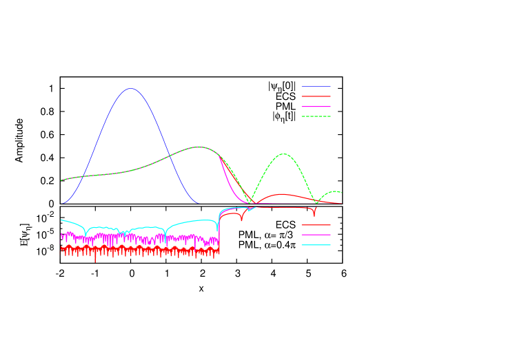
Figure 2: (color online) Relative errors $E(x)$ of $\psi_{\eta}[t]$ at time $t=2.5$ for the TDSE computed with ECS and PML absorption, respectively. The error is defined in Eq. (5.2).

It must be mentioned, though, that we could obtain the very good results only with the exponentially decaying basis at the end intervals. With a standard finite element basis on a finite box we were not able to converge the PML to better than a few percent. Our use of constant stretching by $\Theta_{F}$, rather than a asymptotically growing $\Theta_{F}$, which is customary in PML, may be the reason for this problem. ECS, as was shown in [8], does converge for the TDSE using a finite box, although significantly larger absorption ranges are needed.

6 Conclusion

In this work we have introduced a new unified formulation of the ECS and PML schemes based on spectral analysis. Both methods are mathematically well-defined and heavily rely on analytical continuation. This does not require the solutions to be analytic as functions of the spatial coordinates. In fact, in the present formulation, we admit and explicitly use discontinuities in the $x$-dependence. For transforming to localized representations that exponentially decay at large distances, both methods require that the solutions of the original problem have purely “outgoing” asymptotics. ECS justifiably is called “complex stretching” and ensues a rotation of the spectrum into the complex plane. PML, in contrast, at least for the 1d example treated here, is a “complex gauge transform” and corresponds to a uniform shift of spectral eigenvalues into the lower half complex plane.

Our numerical studies show that the presented mathematical reasoning leads to accurate and stable numerical schemes. We believe that, apart from the specific analysis performed here, the approach based on spectral analysis and analytical continuation of unitary maps will be useful in designing absorption methods also for other wave equations. From a rigorous point of view, the analysis is clearly limited to linear operators. When the equation or a class of solutions can be considered linear at least in some asymptotic sense, the analysis readily provides a first estimate of spectral properties — stability of time-evolution — and asymptotic form — spatially finite approximations of the solution. It is a simple tool to construct the explicit shape of the differential operators and to clarify possible domain questions.

References

- [1] B. Simon. Definition of molecular resonance curves by the method of exterior complex scaling. Phys. Lett. A, 71:211–214, 1979.
- [2] E. Balslev and J. M. Combes. Spectral properties of many-body Schrödinger operators with dilatation-analytic interactions. Communications in Mathematical Physics, 22(4):280–294, December 1971.
- [3] Jean-Pierre Berenger. A perfectly matched layer for the absorption of electromagnetic waves. Journal of Computational Physics, 114(2):185 – 200, 1994.
- [4] Xavier Antoine, Anton Arnold, Christophe Besse, and Achim Ehrhardt, Matthiasand Schädle. A review of transparent and artificial boundary conditions techniques for linear and nonlinear schrodinger equations. Comm. Comp. Phys., 4:729–796, 2008.
- [5] E. Brädas and N. Elander, editors. Resonances, volume 325, Berlin, 1989. Springer.
- [6] Wm. Reinhardt. Complex coordinates in the theory of atomic and molecular structure and dynamics. Ann. Rev. Phys. Chem., 33:223, 1982.
- [7] A. Scrinzi and N. Elander. A finite element implementation of exterior complex scaling. J. Chem. Phys., 98:3866, 1993.
- [8] Armin Scrinzi. Infinite-range exterior complex scaling as a perfect absorber in time-dependent problems. Phys. Rev. A, 81(5):053845, May 2010.
- [9] Weng Cho Chew and William H. Weedon. A 3d perfectly matched medium from modified maxwell’s equations with stretched coordinates. Microwave and Optical Technology Letters, 7(13):599–604, 1994.
- [10] T. Hagström D. Appelö and G. Kreiss. Perfectly matched layers for hyperbolic systems: general formulation, well-posedness, and stability. SIAM J. Appl. Math., 67:1–23, 2006.
- [11] Jacques-Louis Lions, Jérôme Métral, and Olivier Vacus. Well-posed absorbing layer for hyperbolic problems. Numer. Math., 92(3):535–562, 2002.
- [12] Francis Collino. Perfectly matched absorbing layers for the paraxial equations. J. Comput. Phys., 131(1):164–180, February 1997.
- [13] Chunxiong Zheng. A perfectly matched layer approach to the nonlinear Schrödinger wave equations. J. Comput. Phys., 227(1):537–556, 2007.
- [14] Tomáš Dohnal. Perfectly matched layers for coupled nonlinear Schrödinger equations with mixed derivatives. J. Comput. Phys., 228(23):8752–8765, 2009.
- [15] Anna Nissen and Gunilla Kreiss. An optimized perfectly matched layer for the schrödinger equation. Commun. Comput. Phys., 9:147–179, 2011.
- [16] Po-Ru Loh, Ardavan F. Oskooi, Mihai Ibanescu, Maksim Skorobogatiy, and Steven G. Johnson. Fundamental relation between phase and group velocity, and application to the failure of perfectly matched layers in backward-wave structures. Physical Review E, 79:065601(R), June 2009.
- [17] M. Reed and B. Simon. Methods of Modern Mathematical Physics, volume IV. Academic Press, New York, 1982. p. 183.
- [18] A. Scrinzi. Ionization of multielectron atoms by strong static electric fields. Phys. Rev. A, 61:041402(R), 2000.
- [19] A. Saenz. Behavior of molecular hydrogen exposed to strong dc, ac, or low-frequency laser fields. i. bond softening and enhanced ionization. Phys. Rev. A, 66:63407, 2002.
- [20] F. He, C. Ruiz, and a. Becker. Absorbing boundaries in numerical solutions of the time-dependent Schrödinger equation on a grid using exterior complex scaling. Physical Review A, 75(5):1–7, May 2007.
- [21] Liang Tao, W. Vanroose, B. Reps, T. N. Rescigno, and C. W. McCurdy. Long-time solution of the time-dependent schrödinger equation for an atom in an electromagnetic field using complex coordinate contours. Phys. Rev. A, 80(6):063419, Dec 2009.
- [22] Mireille F. Levy. Perfectly matched layer truncation for parabolic wave equation models. R. Soc. Lond. Proc. Ser. A Math. Phys. Eng. Sci., 457(2015):2609–2624, 2001.
- [23] C Farrell and U Leonhardt. The perfectly matched layer in numerical simulations of nonlinear and matter waves. Journal of Optics B: Quantum and Semiclassical Optics, 7(1):1, 2005.
- [24] Tomáš Dohnal and Thomas Hagstrom. Perfectly matched layers in photonics computations: 1d and 2d nonlinear coupled mode equations. Journal of Computational Physics, 223(2):690 – 710, 2007.
- [25] A. Scrinzi and B. Piraux. Two-electron atoms in short intense laser pulses. Phys. Rev. A, 58:1310, 1998.
- [26] Liang Tao and Armin Scrinzi. Photo-electron momentum spectra from minimal volumes: the time-dependent surface flux method. New Journal of Physics, 14(1):013021, 2012.
- [27] Armin Scrinzi. t-surff: fully differential two-electron photo-emission spectra. New Journal of Physics, 14(8):085008, 2012.