Spin-flip transitions and departure from the Rashba model in the Au(111) surface

Abstract

We present a detailed analysis of the spin-flip excitations induced by a periodic time-dependent electric field in the Rashba prototype Au(111) noble metal surface. Our calculations incorporate the full spinor structure of the spin-split surface states and employ a Wannier-based scheme for the spin-flip matrix elements. We find that the spin-flip excitations associated with the surface states exhibit an strong dependence on the electron momentum magnitude, a feature that is absent in the standard Rashba model Rashba (1960). Furthermore, we demonstrate that the maximum of the calculated spin-flip absorption rate is about twice the model prediction. These results show that although the Rashba model accurately describes the spectrum and spin polarization, it does not fully account for the dynamical properties of the surface states.

I INTRODUCTION

Surfaces represent an ideal testing ground for investigating the nature of the relativistic spin-orbit interaction in low dimensional systems Heide et al. (2006); Pascual et al. (2004a); Strozecka et al. (2011). As pointed in the pioneering work by LaShell et al. LaShell et al. (1996), the lack of inversion symmetry of surfaces allows for the spin-splitting of the Shockley-type surface states via the spin-orbit interaction. Noteworthy, the order of magnitude of the energy spin-splitting is as much as $\sim$0.1-0.5 eV, about two orders of magnitude larger than in semiconductors Heide et al. (2006). Recently, several studies performed on coated surfaces have revealed exceptional effects of the spin-orbit interaction. The family of bismuth alloy surfaces Eremeev et al. (2012); Ast et al. (2007); Pascual et al. (2004b), for instance, exhibits giant spin-orbit energy shifts of nearly $400$ meV. Other interesting examples include the semiconducting surfaces Tl/Si(111)$-(1\times 1)$ Sakamoto et al. (2009); Liu and Chang (2009); Ibañez Azpiroz et al. (2011), Tl/Ge(111)$-(1\times 1)$ Ohtsubo et al. (2012) and Yaji et al. (2010); Ibañez Azpiroz et al. (2012) Pb/Ge(111)$-\beta\sqrt{3}\times\sqrt{3}R30\,^{\circ}$, among many others. In these systems, the bulk bands present a gap near the Fermi level, and thus, the electron transport properties are strongly influenced by the spin-split metallic surface states. Even surfaces with light element over-layers such as H/W(110)$-(1\times 1)$ reveal extremely complex spin polarization structure, which is inherent of the anisotropy of the spin-orbit interaction Hochstrasser et al. (2002); Eiguren and Ambrosch-Draxl (2009).

A particularly appealing aspect about surfaces is the possibility of manipulating the electron spin by means of externally applied electric fields Datta and Das (1990); Rashba and Efros (2003); Rashba and Sheka (1961); Golovach et al. (2006); Khomitsky et al. (2012); Rashba (2004). The basic idea in this scenario would be to control the spin orientation by inducing spin-flip excitations between the spin-split surface states. In practice, this is done by applying an external electric field which couples to the spin-dependent electron velocity due to the spin-orbit interaction. Since electric fields are easily created and manipulated experimentally, the mentioned mechanism (electric dipole spin resonance) could offer new perspectives for future applications in spintronics.

In this paper, we present fully relativistic first-principles calculations for analyzing the spin-flip excitations induced by time-dependent electric fields in the Au(111) noble metal surface. This system is considered as the paradigm of a two-dimensional free electron-like gas with the Rashba-type spin-orbit coupling LaShell et al. (1996); Rashba (1960). It is commonly believed that the properties of the Au(111) surface states, such as the energy spin-splitting or the spin polarization structure are well described in terms of the Rashba model Heide et al. (2006); Henk et al. (2004); Liu et al. (2008); Henk et al. (2003); Premper et al. (2007). In fact, the noble metal (111) surfaces have been considered as an almost perfect realization of the Rashba Hamiltonian. However, we demonstrate in this work that the spin related response properties of the Au(111) surface states show a detectable departure from this model. In particular, our calculations demonstrate that the spin-flip transition probability reveals an appreciable angular and momentum dependence, while in the Rashba model this quantity appears with a trivial functional shape. Furthermore, we find that the maximum value of the calculated spin-flip absorption rate is almost double the model prediction.

II THEORETICAL FRAMEWORK

In this section, we briefly introduce the computational approach for analyzing the spin-flip excitations associated with the spin-split surface states. Unless otherwise stated, atomic units will be used throughout the work, $e=\hbar=m_{e}=4\pi\epsilon_{0}=1$. Let us start by considering the following single-particle Hamiltonian including the spin-orbit interaction,

$$\hat{\text{H}}_{0}=\frac{\hat{\textbf{p}}^{2}}{2}-V(\hat{\textbf{r}})-\frac{1}{4c^{2}}\hat{\bm{\sigma}}\cdot\left(\hat{\bm{\nabla}}V(\hat{\textbf{r}})\times{\hat{\textbf{p}}}\right),$$ (1)

where $V(\hat{\textbf{r}})$ is the scalar potential and $\hat{\bm{\sigma}}$ represent the Pauli spin operator. In this framework, we analyze the response of an electron state to an external time-dependent electric field described by the vector potential $\hat{\textbf{A}}_{\text{ext}}(t)=\textbf{A}^{(\alpha)}_{0}\cos\omega t$, where $\omega$ and $\alpha$ represent the frequency and polarization of the external field respectively. The spatial variation of the field is neglected since we are interested in the optical limit ($\textbf{q}\rightarrow 0$), in which case the field can be considered as spatially constant Ibañez Azpiroz et al. (2012); Sherman (2003).

We adopt the following conventions for the $x$ and $y$ linearly polarized, $\textbf{A}^{(x)}_{0}=A_{0}\hat{\textbf{x}}$ and $\textbf{A}^{(y)}_{0}=A_{0}\hat{\textbf{y}}$, and the right (R) and left (L) circularly polarized light, $\textbf{A}_{0}^{(R,L)}=A_{0}(\hat{\textbf{x}}\pm i\hat{\textbf{y}})/\sqrt{2}$ (see Fig. 2a for the axes convention).

In our perturbation theory treatment, the leading term describing the interaction between the external field and the electron gas appears as  Rashba and Efros (2003)

$$\hat{\text{H}}_{\text{int}}(t) = -\frac{1}{c}\hat{\textbf{v}}\cdot\hat{\textbf{A}}_{\text{ext}}(t),$$ (2)

where $\hat{\textbf{v}}$ represents the electron velocity operator, commonly expressed as

$$\hat{\textbf{v}}=-i[\hat{\textbf{r}},\hat{\text{H}}_{\text{0}}]=\dfrac{\partial\hat{\text{H}}_{\text{0}}}{\partial\hat{\textbf{p}}}=\hat{\textbf{p}}-\dfrac{1}{4c^{2}}(\hat{\bm{\sigma}}\times\hat{\bm{\nabla}}V(\hat{\textbf{r}})).$$ (3)

We observe that apart from the canonical contribution $\hat{\textbf{p}}$, the velocity operator contains an additional term which directly depends on the spin. It is precisely due to this term in Eq. 3 that the interaction term in Eq. 2 is allowed to produce spin-flip transitions among spin-split surface states.

The transition rate associated to $\hat{\text{H}}_{\text{int}}(t)$ is calculated considering the ordinary first order perturbation (Fermi’s golden rule),

$$\begin{split}\gamma^{(\alpha)}_{mn}(\omega)=&2\pi\int\left(f_{{\bf k}m}-f_{{\bf k}n}\right)|C^{(\alpha)}_{mn}(\textbf{k})|^{2}\\ &\times\delta(\epsilon_{{\bf k}n}-\epsilon_{\textbf{k}m}-\omega)\frac{d^{2}k}{(2\pi)^{2}}.\end{split}$$ (4)

The above describes transitions from state $m$ to $n$, with $f_{{\bf k}i}$ and $\epsilon_{{\bf k}i}$ the Fermi-Dirac distribution function and surface state eigenvalue, respectively, with $i=m,n$.

The velocity operator, which is the origin of the electron spin-flip transitions, enters the matrix elements in Eq. 4 as

$$\begin{split}C^{(\alpha)}_{mn}(\textbf{k})=-\dfrac{1}{2c}\textbf{A}^{(\alpha)}_{0}\cdot\bra{\Psi_{\textbf{k}m}}\hat{\textbf{v}}\ket{\Psi_{{\bf k}n}},\end{split}$$ (5)

where $\Psi_{\textbf{k}i}(\textbf{r})=e^{i\textbf{k}\cdot\textbf{r}}\cdot u_{\textbf{k}i}(\textbf{r})$ represents the single-particle Bloch spinor wave function of surface states.

Considering the Ehrenfest theorem for the velocity operator, $\hat{\textbf{v}}=-i[\hat{\textbf{r}},\hat{\text{H}}_{\text{0}}]$, and expanding the commutator $[\hat{\textbf{r}},\hat{\text{H}}_{\text{0}}]$, the matrix elements of Eq. 5 can be cast into the following form Blount (1962); Wang et al. (2006),

$$\begin{split}C^{(\alpha)}_{mn}(\textbf{k})=-\dfrac{\epsilon_{{\bf k}n}-\epsilon_{\textbf{k}m}}{2c}\textbf{A}^{(\alpha)}_{0}\cdot\bra{u_{\textbf{k}m}}\hat{\bm{\nabla}}_{\textbf{k}}\ket{u_{{\bf k}n}}.\end{split}$$ (6)

The $\bra{u_{\textbf{k}m}}\hat{\bm{\nabla}}_{\textbf{k}}\ket{u_{{\bf k}n}}$ matrix element is precisely the generalized (non-Abelian) Berry connection Berry (1984) associated to the spin-split surface states.

It is noteworthy that the spin non-collinearity is the ultimate reason why the above term does not vanish, as briefly illustrated in the next lines. Let us begin by considering a system without spin-orbit coupling and subjected to a constant magnetic field along the $z$ axis. In these conditions, the spinor states would be collinearly polarized along the $z$ axis, i.e., we would have $u_{\textbf{k}n}(\textbf{r})=g_{\textbf{k}n}(\textbf{r})\footnotesize\left(\begin{matrix}1\;,\;0\end{matrix}\right)^{\text{T}}$ and $u_{\textbf{k}m}(\textbf{r})=g_{\textbf{k}m}(\textbf{r})\footnotesize\left(\begin{matrix}0\;,\;1\end{matrix}\right)^{\text{T}}$, where T stands for matrix transposition. Since the momentum operator $\hat{\bm{\nabla}}_{\textbf{k}}$ is diagonal in the spin-basis, one deduces that the matrix elements entering Eq. 6 vanish identically. This is in complete contrast to the situation when a finite spin-orbit interaction is present. This interaction induces an explicit momentum dependence of the spinor wave function, $u_{\textbf{k}i}(\textbf{r})=\footnotesize\left(\begin{matrix}g^{+}_{\textbf{k}i}(\textbf{r})\;,\;g^{-}_{\textbf{k}i}(\textbf{r})\end{matrix}\right)^{\text{T}}$. In this case, it is obvious that the spinor $\hat{\bm{\nabla}}_{\textbf{k}}u_{\textbf{k}n}(\textbf{r})=\footnotesize\left(\begin{matrix}\hat{\bm{\nabla}}_{\textbf{k}}g^{+}_{\textbf{k}n}(\textbf{r})\;,\;\hat{\bm{\nabla}}_{\textbf{k}}g^{-}_{\textbf{k}n}(\textbf{r})\end{matrix}\right)^{\text{T}}$ does not generally describe a spin orientation parallel to the original spinor $u_{\textbf{k}n}(\textbf{r})$. Thus, an appreciable magnitude of the $\bra{u_{\textbf{k}m}}\hat{\bm{\nabla}}_{\textbf{k}}\ket{u_{{\bf k}n}}$ matrix elements entering Eq. 6 is a direct consequence of the spin noncollinearity introduced by the spin-orbit interaction. The opposite is also true and one deduces that if the direction of the spin polarization experiences a significant variation in some k-space region, the associated spin-flip matrix elements would accordingly be enhanced, as found in a previous analysis Ibañez Azpiroz et al. (2012).

The calculation of the momentum gradient in Eq. 6 presents a computational challenge because of the inherent phase indeterminacy carried by the spinor wave-functions Blount (1962). As a consequence, simple finite difference formulas cannot be directly applied, and a gauge fixing procedure is needed. Recently, a new method to solve this problem has been presented  Wang et al. (2006); Lopez et al. (2012) whereby the matrix elements are re-expressed in terms of the maximally localized Wannier functions Mostofi et al. (2008). In this scheme, the maximal localization of the Wannier states amounts to obtain the smoothest possible variation of the spinor states within the Brillouin zone, hence the interpolation procedure is optimized. Following this approach, the $C^{\alpha}_{mn}(\textbf{k})$ matrix elements entering Eq. 4 can be interpolated into a very fine k mesh with a negligible computational cost Wang et al. (2006, 2007); Lopez et al. (2012). In the present work, the spin-flip matrix elements and surface state eigenvalues entering the integral of Eq. 4 have been evaluated in a dense $1000\times 1000$ k-point grid. This has allowed to consider a very fine Gaussian width of $4\cdot 10^{-4}$ eV for the integral.

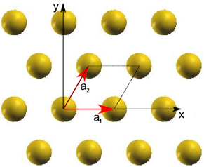
Figure 1: (color online) Top view of the Au(111) surface. Kokalj (2003) Gold atoms are represented by the spheres (yellow). The big (red) arrows denote the 2D direct lattice defined in the text.

The ground state electronic properties of the Au(111) surface have been calculated within the non-collinear LDA-DFT formalism, considering a plane wave basis as implemented in the QUANTUM ESPRESSO package Giannozzi et al. (2009). We used a plane wave cutoff corresponding to $E_{c}=$55 Ry and a $32\times 32$ Monkhorst-Pack mesh Monkhorst and Pack (1976) for the self-consistent cycle. The spin-orbit interaction has been incorporated considering norm-conserving fully relativistic pseudo-potentials for the 5d and 6s electrons of Au, including the full spinor structure of the wave functions Corso and Conte (2005). The Au(111) surface was modeled by the repeated slab technique considering 21 Au layers, with 21 Å of vacuum separating the two sides of the slab and $\sim 2.49$ Å separating adjacent Au layers (interlayer spacing). In this surface, a single 2D lattice is described by the basis vector $\textbf{a}_{1}=a\hat{\textbf{x}}$, $\textbf{a}_{2}=(\hat{\textbf{x}}+\sqrt{3}\hat{\textbf{y}})a/2$, with associated reciprocal basis vectors $\textbf{b}_{1}=2\pi/a(\hat{\textbf{x}}-\hat{\textbf{j}}/\sqrt{3})$, $\textbf{b}_{2}=2\pi/a\cdot 2\hat{\textbf{y}}/\sqrt{3}$, where $a=3.12$ Å. We have included the top view of the surface in Fig. 1. In our optimized configuration, all forces acting on individual atoms were smaller than $1.8\cdot 10^{-4}$ Ry$\cdot$Å^-1.

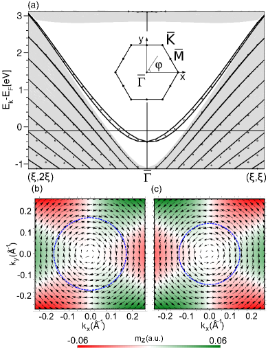
Figure 2: (color online) (a) Band structure of the Au(111) surface close to the $\overline{\Gamma}$ point ($\xi=0.25$ $2\pi/a$). The scalar relativistic and fully relativistic bands are represented by circles and solid lines, respectively. The continuous background (grey) denotes the bulk band projection. (b) and (c) Ab-initio momentum dependent spin polarization associated to lower and higher spin-split sub-bands, respectively. Arrows represent the in-plane spin-polarization component, whereas the background color code indicates the surface perpendicular component, $m_{i,z}(\textbf{k})$. Dashed (blue) lines indicate the calculated ab-initio Fermi surface associated with each surface sub-band. The radii of the circles in (b) and (c) are $k_{F}^{-}$ and $k_{F}^{+}$, respectively.

III RESULTS

III.1 Ground state properties

In Fig. 2a we present the calculated electron band structure of the the Au(111) surface. The scalar relativistic (without spin-orbit interaction) and fully relativistic bands correspond to circles and solid lines, respectively. The bulk band projection is indicated by the background continuum (grey). While the scalar relativistic calculation shows a single spin-degenerate surface band outside the bulk band projection, the fully relativistic calculation shows the two well known spin-split metallic surface state bands measured for the first time by LaShell et al. LaShell et al. (1996) We observe that far from $\overline{\Gamma}$, the spin-split surface bands gradually spin-degenerate as they approach the bulk projection (continuum) and become resonance states. The calculated binding energy at $\overline{\Gamma}$ is 420 meV, while the spin-splitting at the Fermi level ranges approximately from 120 to 135 meV, corresponding to the Fermi wave vectors $k_{F}^{+}=0.145$ $\text{\AA}^{-1}$ and $k_{F}^{-}=0.175$ $\text{\AA}^{-1}$, respectively.

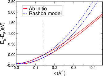
Figure 3: (color online) Comparison between the Rashba model prediction for the energy dispersion (Eq. 14) and the calculated ab-initio band structure of the surface states. The Rashba parameter $\alpha_{R}$ has been fitted at $k_{F}^{+}=0.145$ $\text{\AA}^{-1}$, indicated by the vertical line.

It is instructive to compare the calculated band structure of the surface states with the Rashba model energy dispersion of Eq. 14. This model equation predicts a spin-splitting that grows linearly with the magnitude of the electron momentum, $\Delta E=2|\textbf{k}|\alpha_{R}$, with $\alpha_{R}$ the Rashba parameter. An explicit value for this parameter can be obtained by extracting $\Delta E$ and $|\textbf{k}|$ from the ab-initio band structure. Since we are interested in the details close to the Fermi level, we consider the calculated Fermi wave vector, $|\textbf{k}|=k_{F}^{+}=0.145$ $\text{\AA}^{-1}$, and the corresponding energy spin-splitting, $\Delta E=0.12$ eV, obtaining $\alpha_{R}=\Delta E/2|\textbf{k}|=0.419$ eV$\cdot\text{\AA}$. This value is in good agreement with the one reported in a recent ARPES experiment Henk et al. (2004), $\alpha_{R}=0.396$ eV$\cdot\text{\AA}$. Besides, we obtain an effective mass of $m^{*}=0.23$ (see Eq. 14) from a parabolic fit to the band structure, which also agrees well with experiments Henk et al. (2004), $m^{*}=0.25$.

In Fig. 3 we compare the ab-initio band structure of the surface states with the Rashba model energy dispersion (Eq. 14) calculated using the parameter values $\alpha_{R}=0.419$ eV$\cdot\text{\AA}$ and $m^{*}=0.23$. This figure shows a good agreement for energies below the Fermi level and, as expected, the ab-initio and Rashba model energies coincide exactly at $|\textbf{k}|=k_{F}^{+}$. For $|\textbf{k}|>k_{F}^{+}$, the ab-initio energy spin-splitting of the surface states ceases to grow linearly and, furthermore, it starts decreasing. Therefore, the Rashba model energy dispersion clearly deviates from the ab-initio band structure for $|\textbf{k}|>k_{F}^{+}$.

Figs. 2b and 2c illustrate the momentum dependent spin polarization of the spin-split surface states,

$$\bm{m}_{i}({\bf k})=\int\Psi^{*}_{{\bf k}i}({\bf r})\hat{\bm{\sigma}}\Psi_{{\bf k}i}({\bf r})d^{3}r.$$ (7)

In the figures, arrows represent the in-plane spin-polarization component, while the background code indicates the surface perpendicular component, $m_{z,i}(\textbf{k})$.

Both surface states are spin-polarized in practically the opposite direction in agreement with spin-resolved ARPES measurements LaShell et al. (1996); Henk et al. (2004), and describe a circular spin structure around the $\overline{\Gamma}$ point following the Rashba model (Eq. 13). Our calculations confirm that $\bm{m}_{i}(\textbf{k})$ is almost parallel to the surface for $|\textbf{k}|\lesssim k_{F}^{+}$, which is the region where the Rashba model is expected to properly describe the properties of the surface states. Instead, the calculated surface-perpendicular component ($m_{z,i}(\textbf{k})$) acquires a finite value for $|\textbf{k}|\gtrsim k_{F}^{+}$, indicating a departure from the Rashba model in this region. As shown by Henk et al. Henk et al. (2003), this feature is a consequence of in-plane components of the potential gradient associated with the real surface structure. In our calculations, we find that at $k_{F}^{+}$, the surface-perpendicular component represents the $\sim 3\%$ of the total magnitude of the spin polarization.

III.2 Spin-flip transitions

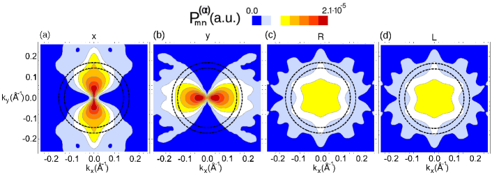
Figure 4: (color online) (a), (b), (c) and (d) Contour plot of the calculated momentum dependent surface state spin-flip transition probability, associated to the incoming light $\alpha=x,y,R$ and $L$ polarizations, respectively. The dashed lines (black) denote the ab-initio calculated Fermi surface associated with the surface states. The radii of the inner and outer circles are $k_{F}^{+}$ and $k_{F}^{-}$, respectively.

Figs. 4a, 4b, 4c and 4d present the calculated momentum dependent spin-flip transition probability associated with the surface states,

$$P^{(\alpha)}_{mn}(\textbf{k})\equiv\dfrac{|C_{mn}^{(\alpha)}(\textbf{k})|^{2}}{|\textbf{A}^{(\alpha)}_{0}|^{2}},$$ (8)

for linearly ($\alpha=x,y$) as well as for circularly ($\alpha=R,L$) polarized light, respectively (see Eq. 5).

In contrast to the Rashba model predicting a constant and totally isotropic transition probability for circularly polarized light (Eq. 23), our calculations presented in Figs. 4c and 4d describe an appreciable hexagonal angular dependence inherited from the C₃ symmetry of the real surface structure. For x and y linearly polarized light, our calculated spin-flip transition probability is in qualitative agreement with the dipole-like function predicted by the Rashba model (Eqs. 21 and 22), but showing again an appreciable modulation.

Noteworthy, our ab-initio calculations show a clear deviation from the Rashba model in one more important aspect; the dependence of the calculated spin-flip transition probability on the momentum magnitude $|\textbf{k}|$. This feature is particularly evident for the x and y linearly polarized light (Figs. 4a and 4b), but it is also present for the R and L circular polarizations (Figs. 4c and 4d). In all these cases, the spin-flip transition probability diminishes with increasing momentum, a feature that is absent in the ideal Rashba model. This can be understood as the surface bands approaching the bulk continuum lose gradually their surface character.

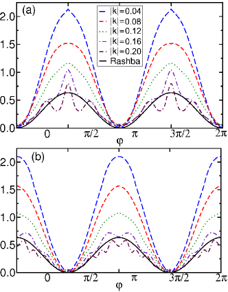
Figure 5: (color online) Calculated angular dependence of the spin-flip transition probability (units of $10^{-5}$ a.u.) for several circular paths corresponding to different absolute values of the electron momentum, $|\textbf{k}|$ (units of Å^-1). Panels (a) and (b) show the results for the incoming $x$ and $y$ linearly polarized light respectively. The solid (black) lines are the $|\textbf{k}|$-independent Rashba model predictions of Eqs. 21 and 22, with the parameter $\alpha_{R}$ extracted from the ab-initio band structure at $k_{F}^{+}$.

In Figs. 5a and 5b we explicitly analyze the angular dependence of the probability distribution for the $x$ and $y$ linearly polarized light, following several circular paths centered at high symmetry point $\overline{\Gamma}$ with fixed momentum $|\textbf{k}|$. We observe that the calculated $P^{(x)}_{mn}(\textbf{k})$ and $P^{(y)}_{mn}(\textbf{k})$ closely follow the dipole-like functional shape of the Rashba model $(\sin^{2}\varphi,\cos^{2}\varphi)$, specially for small momenta, $|\textbf{k}|\lesssim k_{F}^{+}$. We find that even though the order of magnitude coincides for all $|\textbf{k}|$, the calculated spin-flip transition probability shows a remarkable modulation with respect to the Rashba model result near $k_{F}^{+}$.

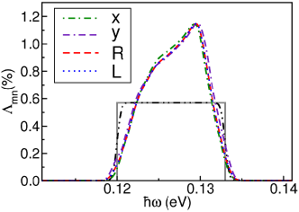
Figure 6: (color online) Integrated spin-flip absorption rate for the Au(111) surface. Super-imposed dashed (red), dotted (blue), dot-dashed (green) and dot-dash-dashed (purple) lines represent the calculated results corresponding to the $x$ and $y$ linear and $R$ and $L$ circularly polarized light, respectively. The constant solid (grey) and dot-dot-dashed (black) lines denote respectively the Rashba model prediction without and with broadening.

In Fig. 6 we present the calculated absorption rate associated to the spin-flip excitations,

$$\Lambda^{(\alpha)}_{mn}(\omega)=\dfrac{\omega\cdot\gamma^{(\alpha)}_{mn}(\omega)}{\mathcal{P}},$$ (9)

where $\gamma^{(\alpha)}_{mn}(\omega)$ is the spin-flip transition rate of Eq. 4, and ${\mathcal{P}}=|\textbf{A}^{(\alpha)}_{0}|^{2}\omega^{2}/8\pi c$ is the optical power per unit area of the incident field. Thus, $\Lambda^{(\alpha)}_{mn}(\omega)$ measures the percentage of the total irradiated light absorbed in the spin-flip processes.

We do not find any significant difference among the $x$ and $y$ linear polarization because of the isotropy of the problem, as the orbital components of the surface states in Au(111) are mainly $s$, $p_{z}$ and $d_{z^{2}}$ Henk et al. (2004); Liu et al. (2008). The results for the $R$ and $L$ circular polarizations superimpose due to the presence of the time reversal symmetry  Souza and Vanderbilt (2008); Yao et al. (2008). The solid (grey) line indicates the constant Rashba model prediction (for zero temperature), $\Lambda_{-+}=\pi/4c\sim 0.57\%$, which is independent of the external field polarization and even of the Rashba parameter $\alpha_{R}$. We deduce from Fig. 6 that light is absorbed in the 120-135 meV energy window, corresponding to the range of the calculated energy spin-splitting of the surface bands close to the Fermi level. Fig. 6 reveals also that the Rashba model underestimates the maximum magnitude of the spin-flip absorption rate by approximately 100%. The reason is that within the Brillouin zone area where spin-flip excitations are allowed ($k_{F}^{+}<|\textbf{k}|<k_{F}^{-}$, see Fig. 4), the calculated values for the transition probability matrix elements are also about twice the ones predicted by the Rashba model.

IV CONCLUSIONS

We have analyzed the spin-flip excitations induced by a time-dependent electric field in the Rashba model textbook example Au(111) surface. We have considered an ab-initio scheme based on maximally localized Wannier functions, including the full spinor structure of the surface states. Remarkably, the calculated ab-initio spin-flip transition probability exhibits an appreciable angular and momentum dependence, showing a much more complex structure than the Rashba model prediction. An important consequence of this modulation is that the maximum of the calculated spin-flip absorption rate is about twice the value predicted by the Rashba model. Thus, even though the Rashba model properly describes the ground state properties of the surface states, these results reveal that it does not fully account for the dynamical properties.

Appendix A SPIN-FLIP TRANSITIONS IN THE RASHBA MODEL

In this appendix we briefly describe the structure of the spin-flip transitions in the Rashba model for a 2D free-electron-like gas Rashba (1960), which is broadly considered as the standard model for analyzing the properties of surface states with spin-orbit interaction Heide et al. (2006). Within this model, electrons are considered as free particles under the action of a simplified spin-orbit coupling,

$$\hat{\text{H}}_{\text{R}}=\alpha_{R}\hat{\bm{\sigma}}\cdot(\hat{\textbf{p}}\times\hat{\textbf{z}}).$$ (10)

Above, $\alpha_{R}$ is the material-dependent Rashba parameter, $\hat{\textbf{p}}=-i\hat{\bm{\nabla}}({\textbf{r}})$ is the electron momentum operator and $\hat{\textbf{z}}$ is a unit vector pointing along the surface-perpendicular direction $z$.

The expression of the Hamiltonian in the Rashba model is given by

$$H_{0}=\dfrac{\hat{\textbf{p}}^{2}}{2m^{*}}+\alpha_{R}\hat{\bm{\sigma}}\cdot(\hat{\textbf{p}}\times\hat{\textbf{z}}),$$ (11)

where $m^{*}$ is the electron effective mass. For an in-plane electron momentum $\textbf{k}=k(\hat{\textbf{x}}\cos\varphi+\hat{\textbf{y}}\sin\varphi)$, the spinor eigenstates of the above Hamiltonian are given by Heide et al. (2006)

$$\Psi_{\textbf{k},\pm}(\textbf{r})=\frac{e^{i\textbf{k}\cdot\textbf{r}}}{2\pi}\frac{1}{\sqrt{2}}\left(\begin{matrix}ie^{-i\varphi/2}\\ \pm e^{i\varphi/2}\\ \end{matrix}\right).$$ (12)

Above, $\pm$ denote the spin-up and spin-down sub-bands. The associated momentum dependent spin polarization is

$$\textbf{m}_{\pm}(\textbf{k})=\Braket{\Psi_{\textbf{k},\pm}}{\bm{\sigma}}{\Psi_{\textbf{k},\pm}}=\frac{1}{2}(\hat{\textbf{x}}\sin\varphi\mp\hat{\textbf{y}}\cos\varphi),$$ (13)

which is perpendicular to both, the electron momentum k and the surface-perpendicular direction $\hat{\textbf{z}}$.

The energy dispersion corresponding to the spinor states of Eq. 12 is

$$\epsilon_{k,\pm}=\dfrac{k^{2}}{2m^{*}}\pm\alpha_{R}k.$$ (14)

Thus, the eigenstates of the Rashba model Hamiltonian show an energy spin-splitting which increases linearly with the electron momentum magnitude,

$$\Delta E_{k}=\epsilon_{k,+}-\epsilon_{k,-}=2\alpha_{R}k.$$ (15)

Due to the Rashba spin-orbit coupling term of Eq. 10, the velocity operator, $\hat{\textbf{v}}=\partial\hat{\text{H}}_{\text{0}}/\partial\hat{\textbf{p}}$ (Eq. 3), becomes spin-dependent,

$$\begin{split}&v_{x}=\dfrac{\hat{p}_{x}}{m^{*}}-\alpha_{R}\hat{\sigma_{y}},\\ &v_{y}=\dfrac{\hat{p}_{y}}{m^{*}}+\alpha_{R}\hat{\sigma_{x}}.\end{split}$$ (16)

Considering the above expressions, the transition matrix elements between the $\Psi_{\textbf{k},\pm}(\textbf{r})$ states (Eq. 5),

$$C^{(\alpha)}_{-+}(\textbf{k})=-\dfrac{e}{2c}\textbf{A}^{(\alpha)}_{\text{0}}\cdot\bra{\Psi_{-\textbf{k}}}\hat{\textbf{v}}\ket{\Psi_{+\textbf{k}}},$$ (17)

are directly accessible.

First, it is worth noting that the spin-diagonal part of the velocity operator (the canonical contribution $\hat{\textbf{p}}/m^{*}$) does not contribute to $C^{(\alpha)}_{-+}(\textbf{k})$ due to the orthogonality of the $\Psi_{\pm\textbf{k}}(\textbf{r})$ states in spin-basis. Therefore, the only finite contribution to $C^{(\alpha)}_{-+}(\textbf{k})$ is proportional to the Pauli matrices appearing in Eq. 16. We find the following expressions for different light polarizations:

$$C^{(x)}_{-+}(\varphi)=\frac{A_{0}}{2c}\bra{\Psi_{-\textbf{k}}}\alpha_{R}\hat{\sigma}_{y}\ket{\Psi_{+\textbf{k}}}=i\frac{\alpha_{R}A_{0}}{2c}\sin\varphi,$$ (18)

$$C^{(y)}_{-+}(\varphi)=-\frac{A_{0}}{2c}\bra{\Psi_{-\textbf{k}}}\alpha_{R}\hat{\sigma}_{x}\ket{\Psi_{+\textbf{k}}}=-i\frac{\alpha_{R}A_{0}}{2c}\cos\varphi,$$ (19)

$$C^{(R,L)}_{-+}(\varphi)=\frac{eA_{0}}{2\sqrt{2}c}\bra{\Psi_{-\textbf{k}}}\alpha_{R}\hat{\sigma}_{y}\mp i\alpha_{R}\hat{\sigma}_{x}\ket{\Psi_{+\textbf{k}}}$$

$$\;\;\;\;\;\;\;\;\;\;\;\;\;\;\;=\pm\frac{\alpha_{R}A_{0}}{2\sqrt{2}c}e^{\mp i\varphi}.$$ (20)

Therefore, the transition matrix elements depend only on the direction of the electron momentum $\varphi$, but not on the magnitude $k$. The associated spin-flip transition probability, $P^{(\alpha)}_{-+}(\textbf{k})\equiv|C_{-+}^{(\alpha)}(\textbf{k})|^{2}/|\textbf{A}^{(\alpha)}_{0}|^{2}$ (see Eq. 8), is straightforwardly obtained from the above expressions,

$$P_{-+}^{(x)}(\varphi)=\dfrac{\alpha_{R}^{2}}{4c^{2}}\sin^{2}\varphi,$$ (21)

$$P_{-+}^{(y)}(\varphi)=\dfrac{\alpha_{R}^{2}}{4c^{2}}\cos^{2}\varphi.$$ (22)

$$P_{-+}^{(R)}=P_{-+}^{(L)}=\dfrac{\alpha_{R}^{2}}{8c^{2}}.$$ (23)

The last equation shows that the transition probability for $R$ and $L$ polarized light is identical and independent of the electron momentum.

Finally, we have all the elements needed to compute the spin-flip absorption rate (Eq. 4),

$$\begin{split}&\Lambda_{-+}^{(\alpha)}(\omega)=\frac{\omega}{\mathcal{P}}2\pi\int\frac{d^{2}k}{(2\pi)^{2}}F_{k}|C^{(\alpha)}_{-+}(\varphi)|^{2}\delta(\Delta E_{k}-\omega)\\ &=\dfrac{4}{c|A_{0}|^{2}\omega}G^{(\alpha)}\int dkF_{k}k\delta(2\alpha_{R}k-\omega),\end{split}$$ (24)

where $F_{k}=f_{k,-}-f_{k,+}$ takes into account the Fermi occupation factors,

$$f_{k,\pm}=\left[\exp\left(\dfrac{k^{2}/2m^{*}\pm\alpha_{R}k-E_{F}}{k_{B}T}\right)+1\right]^{-1},$$ (25)

with $E_{F}$ the Fermi energy, $k_{B}$ the Boltzmann constant and $T$ the temperature. In Eq. 24, $G^{(\alpha)}$ denotes the integration of the angular part, which yields the same result for all light polarizations (see Eqs. 18$-$20),

$$G^{(\alpha)}=\int_{0}^{2\pi}\text{d}\varphi|C^{(\alpha)}_{-+}(\varphi)|^{2}=\dfrac{|A_{0}|^{2}\pi\alpha_{R}^{2}}{4c^{2}}.$$ (26)

Inserting Eq. 26 into Eq. 24 and integrating over $k$, we finally obtain

$$\Lambda_{-+}^{(\alpha)}(\omega)=\dfrac{\pi}{4c}\big{(}f_{\omega,-}-f_{\omega,+}\big{)}.$$ (27)

The spin-flip absorption rate in the Rashba model, Eq. 27, turns out to be independent of the external field polarization. Furthermore, it is almost independent of the Rashba parameter $\alpha_{R}$, which enters only through the occupation factors. Indeed, for $T\rightarrow 0$ we have that

$$\lim_{T\rightarrow 0}\Lambda_{-+}^{(\alpha)}(\omega)=\left\{\begin{array}[]{l l}\dfrac{\pi}{4c}&\quad\text{\small{if} }\omega^{2}/2+\alpha_{R}\omega>E_{F}\\ &\;\;\text{\small{and }}\omega^{2}/2-\alpha_{R}\omega<E_{F},\\ 0&\quad\text{\small{otherwise}}.\end{array}\right.\$$ (28)

Therefore, we conclude that the parameter $\alpha_{R}$ does not affect the magnitude of the light absorption rate, but only the range of frequencies in which light is absorbed.

References

References

- Rashba (1960) E. I. Rashba, Sov. Phys. Solid State 2, 1109 (1960).
- Heide et al. (2006) M. Heide, G. Bihlmayer, P. Mavropoulos, A. Bringer, and S. Blügel, Psi-k Newsletter 78, 1109 (2006).
- Pascual et al. (2004a) J. I. Pascual, G. Bihlmayer, Y. M. Koroteev, H.-P. Rust, G. Ceballos, M. Hansmann, K. Horn, E. V. Chulkov, S. Blügel, P. M. Echenique, et al., Phys. Rev. Lett. 93, 196802 (2004a).
- Strozecka et al. (2011) A. Strozecka, A. Eiguren, and J. I. Pascual, Phys. Rev. Lett. 107, 186805 (2011).
- LaShell et al. (1996) S. LaShell, B. A. McDougall, and E. Jensen, Phys. Rev. Lett. 77, 3419 (1996).
- Eremeev et al. (2012) S. V. Eremeev, I. A. Nechaev, Y. M. Koroteev, P. M. Echenique, and E. V. Chulkov, Phys. Rev. Lett. 108, 246802 (2012).
- Ast et al. (2007) C. R. Ast, J. Henk, A. Ernst, L. Moreschini, M. C. Falub, D. Pacilé, P. Bruno, K. Kern, and M. Grioni, Phys. Rev. Lett. 98, 186807 (2007).
- Pascual et al. (2004b) J. I. Pascual, G. Bihlmayer, Y. M. Koroteev, H.-P. Rust, G. Ceballos, M. Hansmann, K. Horn, E. V. Chulkov, S. Blügel, P. M. Echenique, et al., Phys. Rev. Lett. 93, 196802 (2004b).
- Sakamoto et al. (2009) K. Sakamoto, T. Oda, A. Kimura, K. Miyamoto, M. Tsujikawa, A. Imai, N. Ueno, H. Namatame, M. Taniguchi, P. E. J. Eriksson, et al., Phys. Rev. Lett. 102, 096805 (2009).
- Liu and Chang (2009) M.-H. Liu and C.-R. Chang, Phys. Rev. B 80, 241304 (2009).
- Ibañez Azpiroz et al. (2011) J. Ibañez Azpiroz, A. Eiguren, and A. Bergara, Phys. Rev. B 84, 125435 (2011).
- Ohtsubo et al. (2012) Y. Ohtsubo, S. Hatta, H. Okuyama, and T. Aruga, Journal of Physics: Condensed Matter 24, 092001 (2012).
- Yaji et al. (2010) K. Yaji, Y. Ohtsubo, S. Hatta, H. Okuyama, K. Miyamoto, T. Okuda, A. Kimura, H. Namatame, M. Taniguchi, and T. Aruga, Nat. Commun. 1, 1 (2010).
- Ibañez Azpiroz et al. (2012) J. Ibañez Azpiroz, A. Eiguren, E. Y. Sherman, and A. Bergara, Phys. Rev. Lett. 109, 156401 (2012).
- Hochstrasser et al. (2002) M. Hochstrasser, J. G. Tobin, E. Rotenberg, and S. D. Kevan, Phys. Rev. Lett. 89, 216802 (2002).
- Eiguren and Ambrosch-Draxl (2009) A. Eiguren and C. Ambrosch-Draxl, New Journal of Physics 11, 013056 (2009).
- Datta and Das (1990) S. Datta and B. Das, Appl. Phys. Lett. 56 (1990).
- Rashba and Efros (2003) E. I. Rashba and A. L. Efros, Phys. Rev. Lett. 91, 126405 (2003).
- Rashba and Sheka (1961) E. I. Rashba and V. Sheka, Sov. Phys. Solid State 3, 1357 (1961).
- Golovach et al. (2006) V. N. Golovach, M. Borhani, and D. Loss, Phys. Rev. B 74, 165319 (2006).
- Khomitsky et al. (2012) D. V. Khomitsky, L. V. Gulyaev, and E. Y. Sherman, Phys. Rev. B 85, 125312 (2012).
- Rashba (2004) E. I. Rashba, Phys. Rev. B 70, 201309 (2004).
- Henk et al. (2004) J. Henk, M. Hoesch, J. Osterwalder, A. Ernst, and P. Bruno, Journal of Physics: Condensed Matter 16, 7581 (2004).
- Liu et al. (2008) M.-H. Liu, S.-H. Chen, and C.-R. Chang, Phys. Rev. B 78, 195413 (2008).
- Henk et al. (2003) J. Henk, A. Ernst, and P. Bruno, Phys. Rev. B 68, 165416 (2003).
- Premper et al. (2007) J. Premper, M. Trautmann, J. Henk, and P. Bruno, Phys. Rev. B 76, 073310 (2007).
- Sherman (2003) E. Y. Sherman, Physical Review B 67, 161303 (2003).
- Blount (1962) E. I. Blount, Solid State Physics 13, 305 (1962).
- Wang et al. (2006) X. Wang, J. R. Yates, I. Souza, and D. Vanderbilt, Physical Review B 74, 195118 (2006).
- Berry (1984) M. V. Berry, Proceedings of the Royal Society of London. A. Mathematical and Physical Sciences 392, 45 (1984).
- Lopez et al. (2012) M. G. Lopez, D. Vanderbilt, T. Thonhauser, and I. Souza, Phys. Rev. B 85, 014435 (2012).
- Mostofi et al. (2008) A. A. Mostofi, J. R. Yates, Y. Lee, I. Souza, D. Vanderbilt, and N. Marzari, Computer Physics Communications 178, 685 (2008).
- Wang et al. (2007) X. Wang, D. Vanderbilt, J. R. Yates, and I. Souza, Phys. Rev. B 76, 195109 (2007).
- Kokalj (2003) A. Kokalj, Computational Materials Science 28, 155 (2003).
- Giannozzi et al. (2009) P. Giannozzi, S. Baroni, N. Bonini, M. Calandra, R. Car, C. Cavazzoni, D. Ceresoli, G. L. Chiarotti, M. Cococcioni, I. Dabo, et al., Journal of Physics: Condensed Matter 21, 395502 (2009).
- Monkhorst and Pack (1976) H. J. Monkhorst and J. D. Pack, Phys. Rev. B 13, 5188 (1976).
- Corso and Conte (2005) A. D. Corso and A. M. Conte, Phys. Rev. B 71, 115106 (2005).
- Souza and Vanderbilt (2008) I. Souza and D. Vanderbilt, Phys. Rev. B 77, 054438 (2008).
- Yao et al. (2008) W. Yao, D. Xiao, and Q. Niu, Phys. Rev. B 77, 235406 (2008).