Quantum control robust with coupling with an external environment

Abstract

We study coherent quantum control strategy which is robust with respect to coupling with an external environment. We model this interaction by appending an additional subsystem to the initial system and we choose the strength of the coupling to be proportional to the magnitude of the control pulses. Therefore, to minimize the interaction we impose $L_{1}$ norm restrictions on the control pulses. In order to efficiently solve this optimization problem we employ the BFGS algorithm. We use three different functions as the derivative of the $L1$ norm of control pulses: the signum function, a fractional derivative $\frac{\mathrm{d}^{\alpha}|x|}{\mathrm{d}x^{\alpha}}$, where $0<\alpha<1$, and the Fermi-Dirac distribution. We show that our method allows to efficiently obtain the control pulses which neglect the coupling with an external environment.

I Introduction

The ability to manipulate the dynamics of a given complex quantum system is one of the fundamental issues of the quantum information science. It has been an implicit goal in many fields of science such as quantum physics, chemistry or implementations of quantum information processing d’Alessandro d’Alessandro d’Alessandro (2008); Albertini and D’Alessandro (2002); Werschnik and Gross (2007). The usage of experimentally controllable quantum systems to perform computational task is a very promising perspective. Such usage is possible only if a system is controllable. Thus, the controllability of a given quantum system is an important issue of the quantum information science, since it concerns whether it is possible to drive a quantum system into a previously fixed state.

When manipulating quantum systems, a coherent control strategy is a widely used method. In this case the application of semi-classical potentials, in a fashion that preserves quantum coherence, is used to manipulate quantum states. If a given system is controllable it is interesting to obtain control sequence which drives a system to a desired state and simultaneously minimize the value of the disturbance caused by imperfections of practical implementation. In the realistic implementations of quantum control systems, there can be various factors which disturb the evolution. One of the main issues in this context is decoherence – the fact, that the systems are very sensitive to the presence of the environment, which often destroys the main feature of the quantum dynamics. Other disturbance can be a result of the restriction on the frequency spectrum of acceptable control parameters Pawela and Puchała (2012). In the case of such systems, it is not accurate to apply piecewise-constant controls. In an experimental set up which utilizes an external magnetic field Chaudhury et al. (2007) such restrictions come into play and can not be neglected.

In many situations, the interaction with the control fields causes an undesirable coupling with the environment, which can lead to a destruction of the interesting features of the system. In such situations, it is reasonable to seek a control field with minimal total influence on a system. Depending on a type of interaction with an environment the influence differs. In this article we consider an interaction which is proportional to the magnitude of a control field. To minimize the influence of an environment in such case, when the control field, performs the desired evolution, the $L_{1}$ norm should be minimized.

The paper is organized as follows. In Section II we introduce the model used for simulations. Section III describes the simulation setup. In Section IV we show results of numerical simulations and in Section V we draw the final conclusions.

II Our model

To demonstrate a method of obtaining piecewise-constant controls, which have minimal energy, we will consider an isotropic Heisenberg spin-$1/2$ chain of a finite length $N$. The control will be performed on the first spin only. The total Hamiltonian of the aforementioned quantum control system is given by

$$H(t)=H_{0}+H_{c}(t),$$ (1)

where

$$H_{0}=J\sum_{i=1}^{N-1}(S_{x}^{i}S_{x}^{i+1}+S_{y}^{i}S_{y}^{i+1}+S_{z}^{i}S_{z}^{i+1}),$$ (2)

is a drift part given by the Heisenberg Hamiltonian. The control is performed only on a first spin and is Zeeman-like, i.e.

$$H_{c}(t)=h_{x}(t)S_{x}^{1}+h_{y}(t)S_{y}^{1}.$$ (3)

In the above $S_{k}^{i}$ denotes $k^{\text{th}}$ Pauli matrix which acts on the spin $i$. Time dependent control parameters $h_{x}(t)$ and $h_{y}(t)$ are chosen to be piecewise constant. Furthermore, as opposed to Heule et al. (2010), we do not restrict the control fields to be alternating with $x$ and $y$, i.e. they can be applied simultaneously (see e.g. Khaneja et al. (2005) for similar approach). For notational convenience, we set $\hbar=1$ and after this rescaling frequencies and control-field amplitudes can be expressed in units of the coupling strength $J$, and on the other hand all times can be expressed in units of $1/J$ Heule et al. (2010).

The system described above is operator controllable, as it was shown in Burgarth et al. (2009) and follows from a controllability condition using a graph infection property introduced in the same article. The controllability of the described system can be also deduced from a more general condition utilizing the notion of hypergraphs Puchała (2013).

Since the interest here is focused on operator control sequence, a quality of a control will be measured with the use of gate fidelity,

$$F=\frac{1}{2^{N}}|\mathrm{Tr}(U_{T}^{\dagger}U(h))|,$$ (4)

where $U_{T}$ is the target quantum operation and $U(h)$ is an operation achieved by control parameters $h$. We choose gate fidelity as it neglects global phases.

In the case of disturbed system, we will measure the quality of the control by a trace distance between Choi-Jamiołkowski states, which gives an estimation of a diamond norm.

We introduce an additional constrain on the control pulses, namely we wish to minimize the $L_{1}$ norm of control pulses

$$||h_{k}||_{1}=\sum_{i=1}^{n}|h_{k}^{i}|,$$ (5)

where $k\in\{x,y\}$ and $n$ is the total number of control pulses. In order to make this quantity comparable with fidelity, we impose bounds on the maximal amplitude of the control pulses. To accommodate this, we introduce the following penalty

$$P=\frac{\sum_{i=1}^{n}|h_{k}^{i}|}{nb},$$ (6)

where $b$ is the bound on the control pulse amplitude. This leads to the following functional we wish to minimize

$$G=(1-\mu)P-\mu F,$$ (7)

where $\mu$ is a weight assigned to fidelity.

To optimize the control pulses, we utilize the BFGS algorithm Press et al. (1992). In order to use this method effectively, we need to calculate the explicit form of derivatives of Eq. (5). We propose the following functions to be used as the derivative of the absolute value:

• The signum function:

  $$\frac{\mathrm{d}|x|}{\mathrm{d}x}=\mathrm{sgn}(x).$$ (8)

• A fractional derivative:

  $$\frac{\mathrm{d}^{\alpha}|x|}{\mathrm{d}x^{\alpha}}=\pm\frac{\Gamma(2)}{\Gamma(2-\alpha)}x^{1-\alpha},$$ (9)

  where $\Gamma(x)=(x-1)!$ and we set $\alpha=0.99$.

• The Fermi-Dirac distribution

  $$\frac{\mathrm{d}|x|}{\mathrm{d}x}\approx 2\left(\frac{-1}{\exp(\frac{x}{kT})+}+0.5\right),$$ (10)

  where we set $kT=0.01$.

The signum function is the natural conclusion when one thinks about the derivative of the $L_{1}$ norm as it penalizes any non zero control pulses in the control scheme. To further out studies, we introduce two approximations of the derivative of the $L_{1}$ norm. The first one utilizes the idea of fractional derivatives Miller and Ross (1993). This allows us to achieve a continuous function, which quickly increases from 0 to 1 for positive values of the argument and decreases from 0 to -1 for negative values. Although continuous, the function has the drawback that control pulses with lower magnitude are less penalized. The penalty can be adjusted by using the parameter $\alpha$

The last proposed approximation is the Fermi-Dirac distribution Smirnov (2007). The usage is justified, as for $T=0$ the function is given as

$$f(E)=\left\{\begin{array}[]{rcl}1&\textrm{if}&E<E_{f},\\ 0&\textrm{if}&E>E_{f},\end{array}\right.$$ (11)

where $E_{f}$ is the Fermi energy. From our point of view, the function has properties similar to the fractional derivative and the penalty for low magnitude pulses can be adjusted by using the “temperature” $T$. A comparison of these approximations is shown in Figure 1.

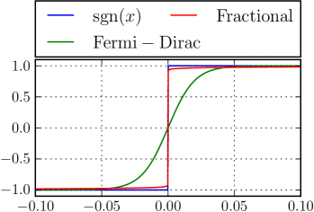
Figure 1: Comparison of different derivative approximations.

III Simulation setup

To demonstrate the beneficialness of our approach, we study three- and four-qubit spin chains. The control field is applied to the first qubit only. Our target gates are:

$$\textrm{NOT}_{N}={\rm 1l}^{\otimes N-1}\otimes\sigma_{x},$$ (12)

the negation of the last qubit of the chain, and

$$\textrm{SWAP}_{N}={\rm 1l}^{\otimes N-2}\otimes\textrm{SWAP},$$ (13)

swapping the states between the last two qubits.

We provide an explicit example in which we set the duration of the control pulse to $\Delta t=0.2$ and the total number of pulses in each direction to $n=64$ for the three-qubit chain and $n=256$ in the four-qubit case, although the presented method may be applied for arbitrary values of $\Delta t$ and $n$. The weight of fidelity in equation (7) is set to $\mu=0.2$ in the three qubit scenario and to $\mu=0.4$ in the four qubit scenario.

IV Results

We show examples of control sequences obtained by using our method in Figs. 2 and 3. They depict results obtained for the three qubit NOT gate optimization and four qubit SWAP gate optimization respectively. In the three qubit scenario we find, as expected, a control sequence which equal to zero most of the time with irregular, high amplitude pulses. A similar case can be made for the swap gate in the four qubit scenario. The main difference is that in this case the high amplitude pulses are surrounded by groups of weaker pulses. The results shown here are for the fractional derivative approximation. Simulations for other approximation yield nearly identical results.

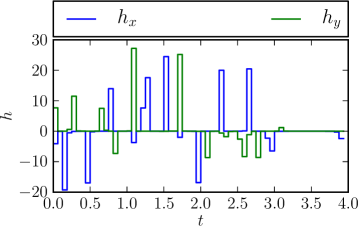
Figure 2: Example control sequences $h_{x}$ and $h_{y}$ for the NOT gate in the three qubit scenario.

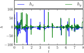
Figure 3: Example control sequences $h_{x}$ and $h_{y}$ for the SWAP gate in the four qubit scenario.

The fidelity obtained in both cases is $F>0.99$ and the value of $P$ has the order of $10^{-2}$.

Finally, we show the evolution of each qubit’s state. Let the qubits be in the state $|\psi\rangle_{0}=|000\rangle$ in the case of the three qubit scenario. Figs. 4, 5 and 6 show the time evolution of each qubit state in this setup. The final state of the chain is $\psi_{f}=|001\rangle$. In the four qubit scenario the time evolution is shown in Figs. 7, 8, 9 and 10. Let the initial state of the chain be equal to $|\phi_{0}\rangle=|0010\rangle$. The final state of the chain is $|\phi\rangle=|0001\rangle$.

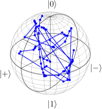
Figure 4: Time evolution of the first qubit of a three qubit chain from the state $|000\rangle$ to the state $|001\rangle$ under the operator ${\rm 1l}\otimes{\rm 1l}\otimes\sigma_{x}$ implemented by optimized control sequences.

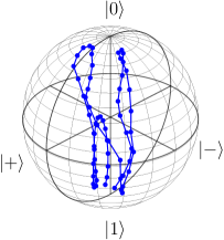
Figure 5: Time evolution of the second qubit of a three qubit chain from the state $|000\rangle$ to the state $|001\rangle$ under the operator ${\rm 1l}\otimes{\rm 1l}\otimes\sigma_{x}$ implemented by optimized control sequences.

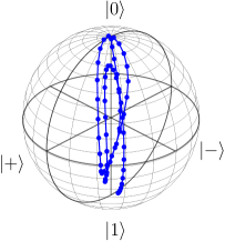
Figure 6: Time evolution of the third qubit of a three qubit chain from the state $|000\rangle$ to the state $|001\rangle$ under the operator ${\rm 1l}\otimes{\rm 1l}\otimes\sigma_{x}$ implemented by optimized control sequences.

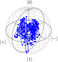
Figure 7: Time evolution of the first qubit of a four qubit chain from the state $|0010\rangle$ to the state $|0001\rangle$ under the operator ${\rm 1l}\otimes{\rm 1l}\otimes\mathrm{SWAP}$ implemented by optimized control sequences.

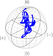
Figure 8: Time evolution of the second qubit of a four qubit chain from the state $|0010\rangle$ to the state $|0001\rangle$ under the operator ${\rm 1l}\otimes{\rm 1l}\otimes\mathrm{SWAP}$ implemented by optimized control sequences.

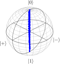
Figure 9: Time evolution of the third qubit of a four qubit chain from the state $|0010\rangle$ to the state $|0001\rangle$ under the operator ${\rm 1l}\otimes{\rm 1l}\otimes\mathrm{SWAP}$ implemented by optimized control sequences.

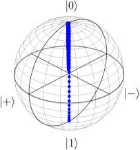
Figure 10: Time evolution of the fourth qubit of a four qubit chain from the state $|0010\rangle$ to the state $|0001\rangle$ under the operator ${\rm 1l}\otimes{\rm 1l}\otimes\mathrm{SWAP}$ implemented by optimized control sequences.

In order to demonstrate the advantages of our approach, we perform additional simulations, where we put $\mu=1$ in Eq. (7). This is the unconstrained problem of finding optimal control pulses. Next, we introduce an interaction with an environment, proportional to $|h_{x}|+|h_{y}|$. We model the interaction with the environment by adding a qubit to the chain. The Hamiltonian for this case is

$$\begin{split}H_{\mathrm{graph}}(t)=&H_{0}+H_{\mathrm{c}}(t)+\gamma(|h_{x}|+|h_{y}|)\times\\ &\times\sum_{i=1}^{N}(S_{x}^{i}S_{x}^{N+1}+S_{y}^{i}S_{y}^{N+1}+S_{z}^{i}S_{z}^{N+1}).\end{split}$$ (14)

In order to compare the evolution with the additional qubit with a given $U_{T}$ we use the following scheme. For a quantum channel $\Phi$, let us write $J(\Phi)$ to denote the associated state:

$$J(\Phi)=\frac{1}{n}\sum_{1\leq i,j\leq n}\Phi(|i\rangle\langle j|)\otimes|i\rangle\langle j|.$$ (15)

Here we are assuming that the channel maps $n\times n$ complex matrices into $m\times m$ complex matrices. The matrix $J(\Phi)$ is sometimes called the Choi-Jamiołkowski representation of $\Phi$. For quantum channels $\Phi_{0}$ and $\Phi_{1}$ we may define the ”diamond norm distance” between them as

$$\|\Phi_{0}-\Phi_{1}\|_{\Diamond}=\sup_{k,\rho}\>\|(\Phi_{0}\otimes{\rm 1l}_{k})(\rho)-(\Phi_{1}\otimes{\rm 1l}_{k})(\rho)\|_{1}$$ (16)

where ${\rm 1l}_{k}$ denotes the identity channel from the set of $k\times k$ complex matrices to itself, $\|\cdot\|_{1}$ denotes the trace norm, and the supremum is taken over all $k\geq 1$ and all density matrices $\rho$ from the set of $nk\times nk$ complex matrices. The supremum always happens to be achieved for some choice of $k\leq n$ and some rank 1 density matrix $\rho$. A coarse bound for the diamond norm defined in Eq. (16) is known Kitaev et al. (2002)

$$\frac{1}{n}\|\Phi_{0}-\Phi_{1}\|_{\Diamond}\leq\|J(\Phi_{0})-J(\Phi_{1})\|_{1}\leq\|\Phi_{0}-\Phi_{1}\|_{\Diamond}.$$ (17)

Therefore, to compare the target operations with and without the additional qubit, we study the $L_{1}$ of the difference of the Jamiołkowski matrices of the respective quantum channels $\|J(\Phi_{0})-J(\Phi_{1})\|_{1}$. The results for different target operations are summarized in Tab. 1. We show results obtained for Fermi-Dirac approximation of the derivative. As stated in the table, the bigger the system under consideration is the greater is the gain from using our method.

	Without additional qubit		With additional qubit
	$\mu=1$	$\mu<1$	$\mu=1$	$\mu<1$
NOT3	0.0000	0.0000	0.0975	0.0086
NOT4	0.0000	0.004	0.9788	0.0142
SWAP3	0.0000	0.0001	0.0135	0.0133
SWAP4	0.0000	0.0020	0.0843	0.0064

Table 1: Summary of the value of Eq. (17) for teh studied cases. For $\mu=1$ we have a control optimization without regarding the $L_{1}$ norm of control pulses.

V Conclusions

In this work we introduced a method of obtaining a piecewise constant control field for a quantum system with an additional constrain of minimizing the $L_{1}$ norm. To demonstrate the beneficialness of our approach, we have shown results obtained for a spin chain, on which we implemented two quantum operations: negation of the last qubit of the chain and swapping the states of the two last qubits of the chain. Our results show that it is possible to obtain control fields which have minimal energy and still give a high fidelity of the quantum operation. Our method may be used in situations where the interaction with the control field causes additional coupling to the environment. As our method allows one to minimize the number of control pulses, it also minimizes the amount of coupling to the environment. Other possible usage of our method includes systems, in which it is possible to use rare, but high value of control pulses, like for example superconducting magnets with high impulse current.