Mixed finite elements for elasticity on quadrilateral meshes

Abstract.

We present stable mixed finite elements for planar linear elasticity on general quadrilateral meshes. The symmetry of the stress tensor is imposed weakly and so there are three primary variables, the stress tensor, the displacement vector field, and the scalar rotation. We develop and analyze a stable family of methods, indexed by an integer $r\geq 2$ and with rate of convergence in the $L^{2}$ norm of order $r$ for all the variables. The methods use Raviart–Thomas elements for the stress, piecewise tensor product polynomials for the displacement, and piecewise polynomials for the rotation. We also present a simple first order element, not belonging to this family. It uses the lowest order BDM elements for the stress, and piecewise constants for the displacement and rotation, and achieves first order convergence for all three variables.

1. Introduction

In this paper we present mixed finite elements for planar linear elasticity which are stable for general quadrilateral meshes. The mixed methods we consider are of the equilibrium type in which the approximate stress tensor $\sigma_{h}$ belongs to $H(\operatorname{div})$ and satisfies the equilibrium condition $\operatorname{div}\sigma_{h}=f$ exactly, at least for loads $f$ which are piecewise polynomial of low degree. However, the methods are based on the mixed formulation of elasticity with weakly imposed symmetry, so that the condition of balance of angular momentum, that is the symmetry of the stress tensor, will be imposed only approximately, via a Lagrange multiplier, which may be interpreted as the rotation. Thus, we consider a formulation in which there are three primary variables, the stress tensor, the displacement vector field, and the scalar rotation. See (1) below.

For this formulation, we propose a family of stable triples of elements, one for each order $r\geq 2$. The lowest order elements, $r=2$, are illustrated in Figure 2. For these we use the second lowest order quadrilateral Raviart-Thomas elements for each row of the stress tensor, discontinuous piecewise bilinear functions for each component of the displacement, and discontinuous piecewise linear functions for the rotation. This method converges with second order in the $L^{2}$ norm for all the variables. We also propose a simpler choice of elements, illustrated in Figure 3. It uses the lowest order rectangular BDM elements for each row of the stress field and piecewise constants for both the displacement and the rotation, and converges with first order in the $L^{2}$ norm for all the variables.

An important point is how the finite element shape functions are transformed from a reference element to an actual quadrilateral element. In order to achieve a stable discretization we use different transformations for the stress, the displacement, and the rotation. The displacement field is simply transformed by composition with the inverse of the bilinear map from the reference element to the quadrilateral, while the stress is mapped by the Piola transform (applied row-by-row). The shape functions for the rotation, in contrast, are not obtained by a transformation from the reference element, but are simply the restriction of polynomials to the actual element.

Mixed finite elements for elasticity have many well-known advantages: robustness with respect to material parameters, applicability to more general constitutive laws such as viscoelasticity, etc. Recently many mixed finite elements have been developed, especially for the formulation in which the symmetry of the stress tensor is imposed weakly (see the next section for a fuller discussion). Stable elements have been developed for both triangles and rectangles. The latter apply easily to parallelograms as well. However, up until now, for the formulation with weakly imposed symmetry condition on the stress field, there have been no stable mixed finite elements available for meshes including general convex quadrilateral elements, even though such meshes are preferred by many practitioners and implemented in many finite element software systems.

Stable pairs of stress and displacement elements for equilibrium mixed formulations of elasticity have been sought since the 1960s. The first elements which were shown to be stable were proposed in [26] and analyzed in [21]. These elements impose symmetry strongly, but they are composite elements, in which the stress elements are piecewise linear with respect to a subdivision into three triangles of each element of the triangular mesh used for the piecewise linear displacements. In [21] a quadrilateral version is analysed as well, in which the stress uses a division into four triangular microelements for each quadrilateral mesh element. The first stable elements with polynomial shape functions were not found for triangular meshes until 2002 [9], and then developed for rectangular meshes in [2]. As far as we know, stable mixed finite elements with strong symmetry and polynomial reference shape functions have not yet been discovered for general quadrilateral meshes.

Because of the difficulty in developing stable mixed methods with strong symmetry, the idea of imposing symmetry weakly was proposed already in 1965 [18]. The first stable elements for this formulation were given in [1] and [5]. Since then numerous stable finite elements with weak symmetry have been developed for simplicial meshes [23, 25, 24, 16], especially since the connection with the de Rham complex and finite element exterior calculus was made in [6, 7]; besides these papers, see [11, 14, 20]. Stable elements for the mixed formulation with weak symmetry have been devised for rectangular meshes as well [22, 10]. The element which we develop in the next section of this paper are, to the best of our knowledge, the first stable mixed finite elements with weak symmetry for general quadrilateral meshes. For a survey of mixed finite elements for elasticity through 2008, we refer to [15].

In the following section we discuss mixed methods based on weakly imposed symmetry in more detail, and recall the conditions required for stable discretization and quasioptimal estimates. In Section 3, we present a framework for the construction of stable elements, based on two main ingredients: the connection between elasticity elements and stable mixed finite elements for the Stokes equation and for the Poisson equation, and the properties of various transformations of scalar, vector, and matrix fields. Based on this framework, in Section 4 we define the finite elements described above and verify their stability. In Section 5, we use the usual tools of mixed methods to obtain improved rates of convergence in $L^{2}$. Finally, in Section 6, we illustrate the performance of the proposed elements with numerical computations.

2. Elasticity with weakly imposed symmetry and its discretization

In this section we recall the weak formulation of the elasticity system based on weak imposition of the symmetry of the stress tensor, and its discretization by Galerkin’s method. We then summarize the basic stability conditions and resulting error estimate for such a method, and present a framework in which stable subspaces can be constructed.

We write $\mathbb{M}$ and $\mathbb{S}$ for the spaces of $2\times 2$ matrices and symmetric matrices, respectively. Let $\Omega$ be a bounded domain in $\mathbb{R}^{2}$ occupied by an elastic body. The material properties are described, at each point $x\in\Omega$, by the compliance tensor $A=A(x)$, a linear operator $\mathbb{S}\to\mathbb{S}$ which is symmetric (with respect to the Frobenius inner product) and positive definite. We shall assume that the compliance tensor is bounded and uniformly positive definite on $\Omega$. We shall also require an extension of $A$ to an operator $\mathbb{M}\to\mathbb{M}$ which is still symmetric and positive definite. This can be obtained, for example, by defining $A$ to act as a positive multiple of the identity on skew-symmetric matrix fields. In the case of a homogeneous and isotropic elastic body,

$$A\sigma=\frac{1}{2\mu}\bigg{(}\sigma-\frac{\lambda}{2\mu+2\lambda}\mathrm{tr}\ (\sigma)I\bigg{)},\quad\sigma\in\mathbb{M},$$

where $I$ is the identity matrix and $\mu>0$ and $\lambda\geq 0$ are the Lamé constants.

Given a vector field $f$ on $\Omega$ encoding the body forces, the equations of static elasticity determine the stress $\sigma:\Omega\to\mathbb{S}$, and the displacement $u:\Omega\to\mathbb{R}^{2}$, satisfying the constitutive equation $A\sigma=\epsilon(u)$, the equilibrium equation $\operatorname{div}\sigma=f$, and boundary conditions, which, for simplicity, we take to be $u=0$ on $\partial\Omega$. Here $\epsilon(u)$ is the symmetric part of the gradient of $u$ and the divergence operator $\operatorname{div}$ applies to the matrix field $\sigma$ row-by-row. Similarly below we shall define $\operatorname{curl}w$ for a vector field $w$ as the matrix field whose first row is $\operatorname{curl}w_{1}$ and second row is $\operatorname{curl}w_{2}$, where $\operatorname{curl}q=(\partial_{2}q,-\partial_{1}q)$ for a scalar function $q$.

To derive the weak formulation of elasticity which we shall use, we write $\operatorname{asym}\tau=\tau_{12}-\tau_{21}$ for the asymmetry of a matrix $\tau\in\mathbb{M}$ and introduce the rotation $p=\operatorname{asym}(\operatorname{grad}u)/2$. The constitutive equation then becomes

$$A\sigma=\operatorname{grad}u-\begin{pmatrix}0&p\\ -p&0\end{pmatrix}.$$

This equation, together with the equilibrium equation and the equation $\operatorname{asym}\sigma=0$ explicitly stating the symmetry of $\sigma$, form the system of differential equations which we shall discretize. For this we shall use the weak formulation, which is to find $(\sigma,u,p)\in H(\operatorname{div},\Omega,\mathbb{M})\times L^{2}(\Omega,\mathbb{R}^{2})\times L^{2}(\Omega)$ such that

(1) $$\begin{split}(A\sigma,\tau)+(u,\operatorname{div}\tau)+(p,\operatorname{asym}\tau)&=0,\quad\tau\in H(\operatorname{div},\Omega,\mathbb{M}),\\ (\operatorname{div}\sigma,v)&=(f,v),\quad v\in L^{2}(\Omega,\mathbb{R}^{2}),\\ (\operatorname{asym}\sigma,q)&=0,\quad q\in L^{2}(\Omega,\mathbb{R}).\end{split}$$

It is convenient to define the space

$$Y=H(\operatorname{div},\Omega,\mathbb{M})\times L^{2}(\Omega,\mathbb{R}^{2})\times L^{2}(\Omega)$$

with the norms

$$\lVert(\tau,v,q)\rVert_{Y}=\lVert\tau\rVert_{H(\operatorname{div})}+\lVert v\rVert_{L^{2}}+\lVert q\rVert_{L^{2}},\quad\lVert(\tau,v,q)\rVert_{L^{2}}=\lVert\tau\rVert_{L^{2}}+\lVert v\rVert_{L^{2}}+\lVert q\rVert_{L^{2}},$$

and to define $B:Y\times Y\to\mathbb{R}$, $F:Y\to\mathbb{R}$ by

(2) $$B(\sigma,u,p;\tau,v,q)=(A\sigma,\tau)+(u,\operatorname{div}\tau)+(p,\operatorname{asym}\tau)+(\operatorname{div}\sigma,v)+(\operatorname{asym}\sigma,q),$$

(3) $$F(\tau,v,p)=(f,v).$$

Note that the bilinear form $B$ is bounded with respect to the $Y$ norm, with the bound depending only on the upper bound for the compliance tensor $A$. In this notation, the weak formulation (1) takes the generic form: find $y=(\sigma,u,p)\in Y$ such that

$$B(y,z)=F(z),\quad z\in Y.$$

We approximate this by Galerkin’s method using finite element spaces $\Sigma_{h}\subset H(\operatorname{div},\Omega,\mathbb{M})$, $V_{h}\subset L^{2}(\Omega,\mathbb{R}^{2})$, and $Q_{h}\subset L^{2}(\Omega)$. Setting $Y_{h}=\Sigma_{h}\times V_{h}\times Q_{h}$, the discrete solution $y_{h}=(\sigma_{h},u_{h},p_{h})\in Y_{h}$ is then defined by

$$B(y_{h},z)=F(z),\quad z\in Y_{h}.$$

We now recall some basic stability and convergence results from the theory of mixed methods. For our problem, Brezzi’s stability conditions [13] are:

• There exists a positive constant $c_{1}$ such that $\lVert\tau\rVert_{H(\operatorname{div})}\leq c_{1}(A\tau,\tau)^{1/2}$ whenever $\tau\in\Sigma_{h}$ satisfies $(\operatorname{div}\tau,v)=0$ for all $v\in V_{h}$ and $(\operatorname{asym}\tau,q)=0$ for all $q\in Q_{h}$.

• There exists a positive constant $c_{2}$ such that for each $v\in V_{h}$ and $q\in Q_{h}$, there is a nonzero $\tau\in\Sigma_{h}$ with

  $$(\operatorname{div}\tau,v)+(\operatorname{asym}\tau,q)\geq c_{2}\lVert\tau\rVert_{H(\operatorname{div})}(\lVert v\rVert_{L^{2}}+\lVert q\rVert_{L^{2}}).$$

These conditions imply the inf-sup condition for the form $B$:

• There exists a positive constant $c_{0}$ (depending on $c_{1}$ and $c_{2}$) such that for each $y\in Y_{h}$ there is a nonzero $z\in Y_{h}$ with $B(y,z)\geq c_{0}\lVert y\rVert_{Y}\lVert z\rVert_{Y}$.

This in turn implies that the Galerkin solution $(\sigma_{h},u_{h},p_{h})$ exists and is unique, and that it satisfies a quasioptimal estimate with respect to the norm in $Y$:

(4) $$\lVert\sigma-\sigma_{h}\rVert_{H(\operatorname{div})}+\lVert u-u_{h}\rVert_{L^{2}}+\lVert p-p_{h}\rVert_{L^{2}}\leq C\inf_{(\sigma,v,q)\in Y_{h}}(\lVert\sigma-\tau\rVert_{H(\operatorname{div})}+\lVert u-v\rVert_{L^{2}}+\lVert p-q\rVert_{L^{2}}),$$

with $C$ depending only on $c_{1}$, $c_{2}$, and an upper bound for $A$. In particular, the constant $C$ is independent of the Lamé parameter $\lambda$ if $c_{1}$ and $c_{2}$ are.

In the next section we study the construction of finite element spaces $\Sigma_{h}$, $V_{h}$, and $Q_{h}$ satisfying (S1) and (S2). First, however, we show that these conditions hold at the continuous level, i.e., when $\Sigma_{h}$ is replaced by $H(\operatorname{div},\Omega,\mathbb{M})$, $V_{h}$ by $L^{2}(\Omega,\mathbb{R}^{2})$, and $Q_{h}$ by $L^{2}(\Omega)$, and so that the weak problem is well-posed. To prove the continuous analogue of (S2), we use the fact that for any $q\in L^{2}(\Omega)$ there exists $w\in H^{1}(\Omega,\mathbb{R}^{2})$ with $\operatorname{div}w=q$ and $\|w\|_{H^{1}}\leq C\|q\|_{L^{2}}$. For example, we may extend $q$ by zero to a smoothly bounded domain and solve the Dirichlet problem for the Poisson equation $\Delta u=q$ on that domain. Then $w=\operatorname{grad}u|_{\Omega}$ has divergence $q$ and satisfies the desired bound.

Now let $v\in L^{2}(\Omega,\mathbb{R}^{2})$ and $q\in L^{2}(\Omega,\mathbb{R})$. Then we can choose $\eta\in H^{1}(\Omega,\mathbb{M})$ such that

$$\operatorname{div}\eta=v,\quad\lVert\eta\rVert_{H^{1}}\leq C\lVert v\rVert_{L^{2}}.$$

Similarly, we can choose $w\in H^{1}(\Omega,\mathbb{R}^{2})$ such that

$$\operatorname{div}w=q-\operatorname{asym}\eta,\quad\lVert w\rVert_{H^{1}} \leq C\lVert q-\operatorname{asym}\eta\rVert_{L^{2}}.$$

If we then set $\tau=\eta-\operatorname{curl}w$, We have

$$\operatorname{div}\tau=\operatorname{div}\eta=v,\quad\operatorname{asym}\tau=\operatorname{asym}\eta+\operatorname{div}w=q.$$

Moreover

$$\lVert\tau\rVert_{H(\operatorname{div})}\leq\lVert\eta\rVert_{H(\operatorname{div})}+\lVert w\rVert_{H^{1}}\leq C(\lVert v\rVert_{L^{2}}+\lVert q\rVert_{L^{2}}),$$

for a constant $C>0$. This suffices to establish (S2) at the continuous level.

The proof of (S1) at the continuous level is simple: the condition $(\operatorname{div}\tau,v)=0$ for all $v\in L^{2}(\Omega,\mathbb{R}^{2})$ means that $\operatorname{div}\tau=0$, so $\lVert\tau\rVert_{H(\operatorname{div})}=\lVert\tau\rVert_{L^{2}}$, which is bounded by a constant multiple of $(A\tau,\tau)^{1/2}$, since the tensor $A$ is positive definite for all $\mu>0$, $\lambda\geq 0$. However, this argument leads to a constant $c_{1}$ which is dependent not only on $\mu$, but also on $\lambda$, and which tends to zero as $\lambda$ tends to infinity, since $A$ loses definiteness in that limit. The standard way to rectify this is to use, instead of the positive definiteness of $A$, the estimate $(A\tau,\tau)\geq(2\mu)^{-1}\|\tau^{D}\|_{L^{2}}^{2}$ where $\tau^{D}$ is the deviatoric or trace-free part $\tau$, and to invoke the bound $\|\tau\|_{L^{2}}\leq c\|\tau^{D}\|_{L^{2}}$ for all $\tau\in H(\operatorname{div},\Omega,\mathbb{M})$ which are divergence-free and which satisfy the additional constraint $\int_{\Omega}\operatorname{tr}\tau\,dx=0$. This argument requires that the solution $\sigma$ satisfies the constraint, for which it suffices to take the test function $\tau$ in (1) to be the constant matrix field everywhere equal to the identity. In this way we may obtain well-posedness uniformly in $\lambda\geq 0$. For details, see, for instance, [5], [11], or [12, Prop. 9.1.1].

3. Construction of stable elements

In view of the preceding section, our goal is to construct finite element spaces $\Sigma_{h}\subset H(\operatorname{div},\Omega,\mathbb{M})$, $V_{h}\subset L^{2}(\Omega,\mathbb{R}^{2})$, and $Q_{h}\subset L^{2}(\Omega)$, satisfying the stability conditions (S1) and (S2). We shall present such spaces in the next section. In Section 3.1, we consider constructions that insure condition (S2), and in Section 3.2, ones that insure (S1).

3.1. The stability condition (S2)

In order to attain (S2), we exploit a connection between stable mixed finite elements for elasticity with weak symmetry and stable mixed finite elements for the Stokes and Poisson equations. This connection, which we recall in Theorem 1, was first observed in [16] and has been elaborated and employed in, for example, [15, 11, 20]. We note that it does not easily generalize to three dimensions.

A pair of spaces $W_{h}\subset H^{1}(\Omega,\mathbb{R}^{2})$, $Q_{h}\subset L^{2}(\Omega)$, is stable for the Stokes equations if it satisfies the appropriate inf-sup condition:

• There exists a positive constant $c_{3}$ such that for each $q\in Q_{h}$ there is a nonzero $w\in W_{h}$ with $(\operatorname{div}w,q)\geq c_{3}\lVert w\rVert_{H^{1}}\lVert q\rVert_{L^{2}}$.

Numerous stable Stokes pairs are known, and in Section 4 we shall choose from among them in order to fulfil (S3).

It is also useful to recall an equivalent form of (S3).

Lemma 1.

The inf-sup condition (S3) holds for some positive constant $c_{3}$ if and only if for all $q\in Q_{h}$ there exists $w\in W_{h}$ such that $P_{Q_{h}}\operatorname{div}w=q$ and $\lVert w\rVert_{H^{1}}\leq c_{3}^{-1}\lVert q\rVert_{L^{2}}$, where $P_{Q_{h}}:L^{2}(\Omega)\to Q_{h}$ is the $L^{2}$-projection.

Proof.

Let $L_{h}=P_{Q_{h}}\operatorname{div}|_{W_{h}}:W_{h}\to Q_{h}$, and let $L_{h}^{*}:Q_{h}\to W_{h}$ be its Hilbert space adjoint, where, as norms on $W_{h}$ and $Q_{h}$ we use the $H^{1}$ and $L^{2}$ norms, respectively. Note that

$$\sup_{w\in W_{h}}\frac{(\operatorname{div}w,q)}{\lVert w\rVert_{H^{1}}}=\sup_{w\in W_{h}}\frac{(L_{h}w,q)_{Q_{h}}}{\lVert w\rVert_{W_{h}}}=\sup_{w\in W_{h}}\frac{(w,L_{h}^{*}q)_{W_{h}}}{\lVert w\rVert_{W_{h}}}=\lVert L_{h}^{*}q\rVert_{W_{h}},$$

so condition (S3) states that

$$\lVert L_{h}^{*}q\rVert_{W_{h}}\geq c_{3}\lVert q\rVert_{Q_{h}},\quad q\in Q_{h},$$

which is equivalent to stating that $L_{h}^{*}$ is an injective map of $Q_{h}$ onto a subspace of $W_{h}$ with inverse bounded by $c_{3}^{-1}$. This in turn is equivalent to the statement that $L_{h}$ is a surjective map of $W_{h}$ onto $Q_{h}$ and admits a right-inverse bounded by $c_{3}^{-1}$, which is the desired condition.∎∎

For the mixed Poisson equation, the inf-sup condition uses the $H(\operatorname{div})$ norm rather than the $H^{1}$ norm. That is, a pair of spaces $S_{h}\subset H(\operatorname{div},\Omega,\mathbb{R}^{2})$, $U_{h}\subset L^{2}(\Omega)$ are required to satisfy the condition:

• There exists a positive constant $c_{4}$ such that for each $q\in U_{h}$ there is a nonzero $w\in S_{h}$ with $(\operatorname{div}w,q)\geq c_{4}\lVert w\rVert_{H(\operatorname{div})}\lVert q\rVert_{L^{2}}$.

Again, there are numerous pairs of spaces known to satisfy (S4). The next theorem gives the connection to mixed elasticity elements. It states that, if we choose a pair of spaces satisfying (S3) and another satisfying (S4), and if the two choices satisfy the compatibility condition (5) below, then we obtain spaces satisfying (S2).

Theorem 1.

Suppose that $W_{h}\subset H^{1}(\Omega,\mathbb{R}^{2})$ and $Q_{h}\subset L^{2}(\Omega)$ satisfy (S3) and that $S_{h}\subset H(\operatorname{div},\Omega,\mathbb{R}^{2})$ and $U_{h}\subset L^{2}(\Omega)$ satisfy (S4). Suppose further that

(5) $$\operatorname{curl}W_{h}\subset S_{h}\times S_{h}.$$

Then $\Sigma_{h}:=S_{h}\times S_{h}\subset H(\operatorname{div},\Omega,\mathbb{M})$ and $V_{h}:=U_{h}\times U_{h}\subset L^{2}(\Omega,\mathbb{R}^{2})$ and $Q_{h}\subset L^{2}(\Omega)$ satisfy (S2).

Proof.

Let $v\in V_{h}$, $q\in Q_{h}$ be given. Since $\Sigma_{h}=S_{h}\times S_{h}$ and $V_{h}=U_{h}\times U_{h}$, (S4) implies that there exists $\eta\in\Sigma_{h}$ such that

$$(\operatorname{div}\eta,v)=\lVert v\rVert_{L^{2}}^{2},\quad\lVert\eta\rVert_{H(\operatorname{div})}\leq c_{4}^{-1}\lVert v\rVert_{L^{2}}.$$

Next we invoke (S3) with $q$ replaced by $q-P_{Q_{h}}(\operatorname{asym}\eta)$. By Lemma 1, there exists $w\in W_{h}$ such that

$$P_{Q_{h}}(\operatorname{div}w)=q-P_{Q_{h}}(\operatorname{asym}\eta),\quad\lVert w\rVert_{H^{1}}\leq c_{3}^{-1}(\lVert q\rVert_{L^{2}}+\lVert\eta\rVert_{L^{2}}).$$

Set

$$\tau=\eta-\operatorname{curl}w\in\Sigma_{h}.$$

Then

$$(\operatorname{div}\tau,v)=(\operatorname{div}\eta,v)=\lVert v\rVert_{L^{2}}^{2}.$$

Also, since $\operatorname{asym}(\operatorname{curl}w)=-\operatorname{div}w$,

$$(\operatorname{asym}\tau,q) =(\operatorname{asym}\eta,q)+(\operatorname{div}w,q)$$

$$=(P_{Q_{h}}(\operatorname{asym}\eta),q)+(q-P_{Q_{h}}(\operatorname{asym}\eta),q)=\lVert q\rVert_{L^{2}}^{2},$$

and

$$\lVert\tau\rVert_{H(\operatorname{div})}\leq\lVert\eta\rVert_{H(\operatorname{div})}+\lVert w\rVert_{H^{1}}\leq C(\lVert v\rVert_{L^{2}}+\lVert q\rVert_{L^{2}}),$$

where $C$ depends only on $c_{3}$ and $c_{4}$. This completes the verification of (S2). ∎∎

3.2. The stability condition (S1)

The key to obtaining (S1) will be the construction of the finite element spaces $\Sigma_{h}$ and $V_{h}$ from shape function spaces $\hat{\Sigma}\subset H(\operatorname{div},\hat{K},\mathbb{M})$ and $\hat{V}\subset L^{2}(\hat{K},\mathbb{R}^{2})$ on a reference element $\hat{K}$, which are transformed to a general element using appropriate transformations. We define these transformations now and summarize their main properties in Lemma 8 below. Based on these we establish (S1) in Theorem 2.

Suppose that $F_{K}:\hat{K}\to K$ is a diffeomorphism of bounded domains in the plane. (In the applications in the next section, $\hat{K}$ will be the unit square and $F_{K}$ will be an invertible bilinear map onto a convex quadrilateral $K$.) A scalar- or vector-valued function $\hat{q}$ on $\hat{K}$ transforms to a function $P_{K}^{0}\hat{q}$ on $K$ by composition:

$$P_{K}^{0}\hat{q}(x)=\hat{q}(\hat{x}),$$

where $x=F_{K}(\hat{x})$. A different way to transform a scalar- or vector-valued function brings in the Jacobian determinant $J_{K}=\det\operatorname{grad}F_{K}$:

$$P_{K}^{2}\hat{q}(x)=\frac{1}{J_{K}(\hat{x})}\hat{q}(\hat{x}).$$

The notation refers to exterior calculus: $P_{K}^{0}$ corresponds to pull back by $F_{K}^{-1}$ if we think of $\hat{q}$ as a differential $0$-form on $\hat{K}$, and $P_{K}^{2}$ corresponds to pull back as a $2$-form. A third way to transform a vector-valued function is to treat it as a $1$-form, i.e., to use the Piola transform:

(6) $$P_{K}^{1}\hat{v}(x)=\frac{1}{J_{K}(\hat{x})}[\operatorname{grad}F_{K}(\hat{x})]\hat{v}(\hat{x}).$$

We can also transform a matrix-valued function on $\hat{K}$ to one on $K$ by applying the Piola transform to each row. This transformation will also be denoted by $P_{K}^{1}$. We have the following fundamental identities.

Lemma 2.

(7) $$\operatorname{curl}P_{K}^{0}\hat{v}=P_{K}^{1}(\operatorname{curl}\hat{v}),\quad\operatorname{div}P_{K}^{1}\hat{\tau}=P_{K}^{2}(\operatorname{div}\hat{\tau}),$$

and

(8) $$(P_{K}^{2}\hat{q},P_{0}\hat{v})_{L^{2}(K)}=(\hat{q},\hat{v})_{L^{2}(\hat{K})},\quad(\operatorname{div}P_{K}^{1}\hat{\tau},P_{K}^{0}\hat{v})_{L^{2}(K)}=(\operatorname{div}\hat{\tau},\hat{v})_{L^{2}(\hat{K})}.$$

Proof.

The above relationships follow naturally in exterior calculus, or can be verified by elementary vector calculus. ∎∎

Now, let $\hat{K}\subset\mathbb{R}^{2}$ be a fixed reference element (e.g., the unit square), and suppose that ${\mathcal{T}}_{h}$ is a partition of $\Omega$ into finite elements such that for each $K\in{\mathcal{T}}_{h}$ there is given a diffeomorphism $F_{K}$ of $\hat{K}$ onto $K$. Suppose we are given a reference shape function space $\hat{V}\subset L^{2}(\hat{K},\mathbb{R}^{2})$ and that the finite element space $V_{h}$ is defined by

(9) $$V_{h}=\{\,v\in L^{2}(\Omega,\mathbb{R}^{2})\,:\,v|_{K}\in P_{K}^{0}\hat{V},\ \forall K\in\mathcal{T}_{h}\,\}.$$

Further assume given a reference shape function space $\hat{\Sigma}\subset H(\operatorname{div},\hat{K},\mathbb{M})$ and suppose that the finite element space $\Sigma_{h}$ satisfies

(10) $$\Sigma_{h}=\{\,\tau\in H(\operatorname{div},\Omega,\mathbb{M})\,:\,\tau|_{K}\in P_{K}^{1}\hat{\Sigma},\ \forall K\in{\mathcal{T}}_{h}\,\}.$$

Finally, assume that the shape function spaces are related by the inclusion

(11) $$\operatorname{div}\hat{\Sigma}\subset\hat{V}.$$

These conditions imply (S1).

Theorem 2.

If the shape function spaces $\hat{V}$ and $\hat{\Sigma}$ satisfy (11), and the finite element spaces $V_{h}$ and $\Sigma_{h}$ are defined by (9) and (10), then (S1) holds.

Proof.

It is certainly sufficient to prove that if $\tau\in\Sigma_{h}$ and $(\operatorname{div}\tau,v)=0$ for all $v\in V_{h}$, then $\operatorname{div}\tau=0$. Indeed, this property implies (S1).

Pick $K\in{\mathcal{T}}_{h}$ and set $\hat{\tau}=(P_{K}^{1})^{-1}(\tau|_{K})$, $\hat{v}=\operatorname{div}\hat{\tau}$. By (10), $\hat{\tau}\in\hat{\Sigma}$, and by (11), $\hat{v}\in\hat{V}$. Define $v\in L^{2}(\Omega,\mathbb{R}^{2})$ by $v|_{K}=(P_{K}^{0})^{-1}\hat{v}$, and $v\equiv 0$ on $\Omega\setminus K$. By (9), $v\in V_{h}$, and so, by assumption, $(\operatorname{div}\tau,v)=0$. Using (8),

$$(\operatorname{div}\tau,v)=(\operatorname{div}\tau|_{K},v|_{K})_{L^{2}(K)}=(\operatorname{div}\hat{\tau},\hat{v})_{L^{2}(\hat{K})}=\lVert\operatorname{div}\hat{\tau}\rVert_{L^{2}(\hat{K})}^{2}.$$

Thus $\operatorname{div}\hat{\tau}=0$, and so, with (7) $\operatorname{div}\tau|_{K}=P_{K}^{2}(\operatorname{div}\hat{\tau})=0$. Since $K$ was arbitrary, this shows that $\operatorname{div}\tau$ vanishes, as desired. ∎∎

Remark 1.

This argument leads to the constant $c_{1}$ in (S1) depending on both $\lambda$ and $\mu$. Just as for the continuous case discussed at the end of Section 2, a slightly more elaborate argument shows that $c_{1}$ can be taken independent of $\lambda$. For this we need to choose the test function $\tau$ equal to the constant identity matrix in order to show that the $\sigma_{h}$ satisfies the constraint $\int\operatorname{tr}\sigma_{h}\,dx=0$. Thus we have to check that the constant identity matrix field belongs to $\Sigma_{h}$. From the definition (10) this means checking that $(P^{1}_{K})^{-1}I\in\hat{\Sigma}$, i.e., that $J_{K}(\hat{x})[\operatorname{grad}F_{K}(\hat{x})]^{-1}\in\hat{\Sigma}$. Now $J_{K}(\hat{x})[\operatorname{grad}F_{K}(\hat{x})]^{-1}$ is the transposed matrix of cofactors of the Jacobian matrix $\operatorname{grad}F_{K}(\hat{x})$. Since the components of $F_{K}(\hat{x})$ are bilinear, the cofactors are linear polynomials. Thus, as long as the reference space function space $\hat{\Sigma}$ contains the space ${\mathcal{P}}_{1}(\hat{K},\mathbb{M})$, then Theorem 2 results in (S1) holding with constant $c_{1}$ independent of $\lambda$, and the resulting mixed method will not exhibit locking for nearly incompressible materials. This is the case for all of the choices of $\hat{\Sigma}$ we make below.

4. Stable elements for elasticity

Theorems 1 and 2 give strong guidance on the construction of stable spaces $\Sigma_{h}$, $V_{h}$, and $Q_{h}$ for elasticity. First, we require spaces $W_{h}$, $Q_{h}$, $S_{h}$, $U_{h}$ which satisfy the hypotheses of Theorem 1, i.e., the first two form a stable pair for the Stokes equations and the latter two a stable pair for the mixed Poisson equation, and the compatibility condition (5) is satisfied. In order that the hypothesis of Theorem 2 are also met, we will construct these four spaces starting with shape functions on a reference element using appropriate transformations. Finally, we take $\Sigma_{h}=S_{h}\times S_{h}$, $V_{h}=U_{h}\times U_{h}$, and $Q_{h}$ as our elements for the stress, displacement, and rotation. Note that the space $W_{h}$ (the Stokes velocity space) is only used for the analysis, and does not enter the mixed method for elasticity.

We henceforth denote by $\hat{K}$ the unit square, and we assume that the partition ${\mathcal{T}}_{h}$ of $\Omega$ consists of convex quadrilaterals $K$, and that each $F_{K}$ is a bilinear isomorphism of $\hat{K}$ onto $K$. We assume that ${\mathcal{T}}_{h}$ is shape regular in the sense of [19, p. 105]. To define this, we consider for each convex quadrilateral the four triangles obtained by connecting three of its vertices and let $\rho_{K}$ be the smallest of the diameters of the corresponding inscribed circles. A sequence of quadrilateral meshes is shape regular if there is a constant $\sigma$ such that $\operatorname{diam}(K)/\rho_{K}\leq\sigma$ for all the elements in the meshes.

4.1. A first choice of elements

Let ${\mathcal{P}}_{r}$ denote the space of polynomials of degree at most $r$, and ${\mathcal{P}}_{r,s}$ the space of polynomials of degree at most $r$ in $x_{1}$ and $s$ in $x_{2}$. We write ${\mathcal{Q}}_{r}$ for ${\mathcal{P}}_{r,r}$, and ${\mathcal{R}\mathcal{T}}_{r}={\mathcal{P}}_{r,r-1}\times{\mathcal{P}}_{r-1,r}$. The last space consists of the shape functions for the Raviart–Thomas space on a square. For $K\subset\mathbb{R}^{2}$ we write ${\mathcal{P}}_{r}(K)$ for functions on $K$ obtained by restriction of polynomials in ${\mathcal{P}}_{r}$, and use a similar notation for the other spaces.

For our first choice of elements, the vector-valued finite element spaces $W_{h}$ and $S_{h}$ will be constructed starting from reference shape function spaces:

$$\hat{W}={\mathcal{Q}}_{2}(\hat{K})\times{\mathcal{Q}}_{2}(\hat{K}),\quad\hat{S}={\mathcal{R}\mathcal{T}}_{2}(\hat{K}).$$

These satisfy

(12) $$\operatorname{curl}\hat{W}\subset\hat{S}\times\hat{S}.$$

We then set

(13) $$W_{h} =\{\,w\in H^{1}(\Omega,\mathbb{R}^{2})\,:\,w|_{K}\in P_{K}^{0}\hat{W},\ \forall K\in{\mathcal{T}}_{h}\,\},$$

(14) $$S_{h} =\{\,s\in H(\operatorname{div},\Omega,\mathbb{R}^{2})\,:\,s|_{K}\in P_{K}^{1}\hat{S},\ \forall K\in{\mathcal{T}}_{h}\,\}.$$

Note that the transform $P_{K}^{0}$ is used to define $W_{h}$, but the Piola transform $P_{K}^{1}$ is used in the definition of $S_{h}$. Using (12) and the first property in (7) of the transformations, we see that the crucial compatibility condition (5) is satisfied.

The scalar-valued space $U_{h}$ is also defined starting with reference shape functions. We choose $\hat{U}={\mathcal{Q}}_{1}$ and define

(15) $$U_{h}=\{\,u\in L^{2}(\Omega)\,:\,u|_{K}\in P_{K}^{0}\hat{U},\ \forall K\in{\mathcal{T}}_{h}\,\}.$$

In contrast, the scalar-valued space $Q_{h}$ is defined directly using polynomials on the elements of ${\mathcal{T}}_{h}$ with no interelement continuity:

$$Q_{h}=\{\,q\in L^{2}(\Omega)\,:\,q|_{K}\in{\mathcal{P}}_{1}(K),\ \forall K\in{\mathcal{T}}_{h}\,\}.$$

Each of the spaces $W_{h}$, $Q_{h}$, $S_{h}$, $U_{h}$ has a standard set of degrees of freedom which enforce the desired degree of continuity for the assembled spaces $W_{h}$, $Q_{h}$, $S_{h}$, and $U_{h}$. For $\hat{W}$ the degrees of freedom are the values of both components at the vertices of the square, the integral of both components on the edges, and the integral of both components over the square. For $\hat{S}$ they are the averages and first moments of the normal component on each edge and the interior moments weighted by ${\mathcal{P}}_{0,1}\times{\mathcal{P}}_{1,0}$. For $\hat{Q}$ and $\hat{U}$ all the degrees of freedom are interior. Figure 1 illustrates the degrees of freedom for the four spaces, and also includes an indication of how the shape functions transform to the reference element for each space. Note that the functions in $W_{h}$ are vector fields, so each of the dots in the corresponding diagram represent two degrees of freedom.

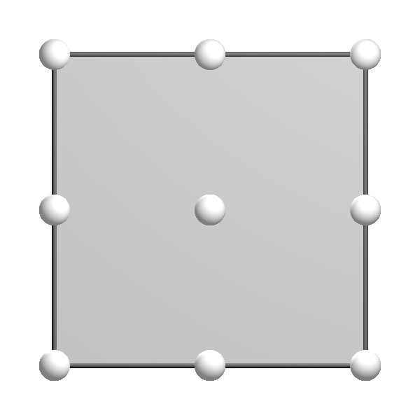
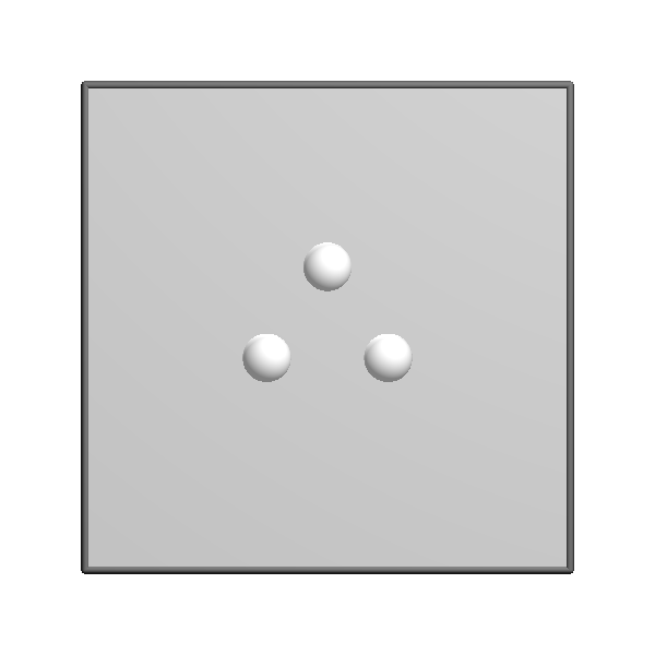
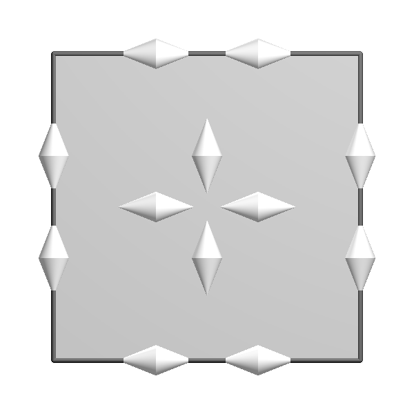
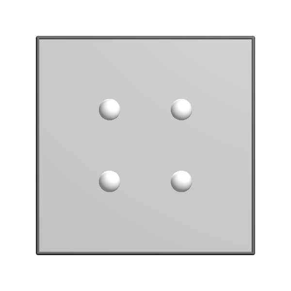
$W_{h}$ ($P_{K}^{0}$) $Q_{h}$ (unmapped) $S_{h}$ ($P_{K}^{1}$) $U_{h}$ ($P_{K}^{0}$) ${\mathcal{Q}}_{2}\times{\mathcal{Q}}_{2}$ ${\mathcal{P}}_{1}$ ${\mathcal{R}\mathcal{T}}_{2}$ ${\mathcal{Q}}_{1}$ $\underbrace{\hskip 156.49014pt}_{\text{\normalsize Stokes}}$ $\underbrace{\hskip 156.49014pt}_{\text{\normalsize mixed Poisson}}$

Figure 1. Degrees of freedom and transformations used to construct the first elements.

The Stokes pair $W_{h}$, $Q_{h}$ is a standard Stokes element, the $Q_{2}$–$P_{1}$ element, for which the inf-sup condition (S3) is well known. See [19, Chapter II, §3.2]. The mixed Poisson pair $S_{h}$, $U_{h}$ is a standard choice as well, the quadrilateral Raviart–Thomas elements of second lowest order. A proof of the inf-sup condition (S4) for general quadrilateral meshes is given, e.g., in [4]. We have thus verified the hypotheses of Theorem 1. Therefore if we define $\Sigma_{h}=S_{h}\times S_{h}$ and $V_{h}=U_{h}\times U_{h}$, the triple $\Sigma_{h}$, $V_{h}$, $Q_{h}$ satisfies (S2).

From the definitions of $S_{h}$ and $U_{h}$, it follows that (9) holds with $\hat{V}=\hat{U}\times\hat{U}$ and (10) holds with $\hat{\Sigma}=\hat{S}\times\hat{S}$. Since $\operatorname{div}\hat{S}\subset\hat{U}$, (11) holds. Theorem 2 thus applies, showing that the spaces $\Sigma_{h}$, $V_{h}$, $Q_{h}$ satisfy (S1) as well. Thus we have indeed constructed a stable triple of spaces for the elasticity problem, satisfying the stability condition (S0) and therefore the quasioptimality estimate (4). The diagram for the elements are shown in Figure 2.

stress $\Sigma_{h}$ ($P_{K}^{1}$) displacement $V_{h}$ ($P_{K}^{0}$) rotation $Q_{h}$ (unmapped) ${\mathcal{R}\mathcal{T}}_{2}\times{\mathcal{R}\mathcal{T}}_{2}$ ${\mathcal{Q}}_{1}\times{\mathcal{Q}}_{1}$ ${\mathcal{P}}_{1}$

Figure 2. The first choice of elasticity elements.

4.2. Higher order elements

The above elements generalize directly to arbitrary order $r\geq 2$. For the Stokes element we use ${\mathcal{Q}}_{r}$-${\mathcal{P}}_{r-1}$, and for the mixed Poisson element we use ${\mathcal{R}\mathcal{T}}_{r}$-${\mathcal{Q}}_{r-1}$.

4.3. A simpler element

In this section we derive a simpler element. The stress is approximated by the lowest order quadrilateral BDM elements, which is constructed from an $8$-dimensional space ${\mathcal{B}\mathcal{D}\mathcal{M}}_{1}$ of reference shape functions, spanned by ${\mathcal{P}}_{1}$ vector fields together with the two vector fields $\operatorname{curl}\hat{x}_{1}^{2}x_{2}$ $\operatorname{curl}\hat{x}_{1}x_{2}^{2}$. The displacement and rotation spaces simply consist of piecewise constants. This element is thus a quadrilateral analogue of the simple triangular finite element for elasticity with weak symmetry introduced in [6] and [8]. The elasticity element is summarized in Figure 3.

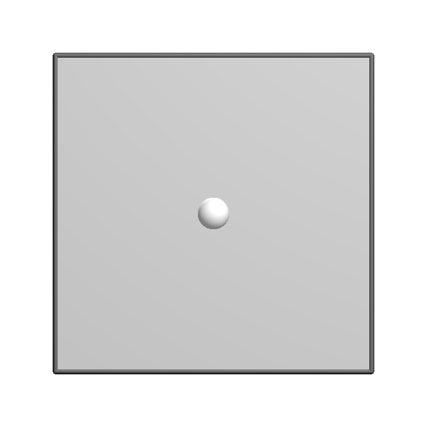
stress $\Sigma_{h}$ ($P_{K}^{1}$) displacement $V_{h}$ rotation $Q_{h}$ ${\mathcal{B}\mathcal{D}\mathcal{M}}_{1}\times{\mathcal{B}\mathcal{D}\mathcal{M}}_{1}$ ${\mathcal{P}}_{0}\times{\mathcal{P}}_{0}$ ${\mathcal{P}}_{0}$

Figure 3. A simple stable choice of elasticity elements.

Note that the mixed Poisson gradient space is based on ${\mathcal{B}\mathcal{D}\mathcal{M}}_{1}$ rather than ${\mathcal{R}\mathcal{T}}_{2}$ as in the first element. For analysis, we define the Stokes velocity space using the serendipity space $\SS_{2}$ instead of ${\mathcal{Q}}_{2}$. The space of serendipity polynomials $\SS_{r}$ is defined to be the span of ${\mathcal{P}}_{r}$ and the two polynomials $x_{1}^{r}x_{2}$ and $x_{2}x_{2}^{r}$, and the space ${\mathcal{B}\mathcal{D}\mathcal{M}}_{r}$ is the span of ${\mathcal{P}}_{r}\times{\mathcal{P}}_{r}$ and the two vector fields $\operatorname{curl}x_{1}^{r+1}x_{2}$ and $\operatorname{curl}x_{1}x_{2}^{r+1}$. Thus, for this element, the reference shape functions are

$$\hat{W}=\SS_{2}(\hat{K})\times\SS_{2}(\hat{K}),\quad\hat{S}={\mathcal{B}\mathcal{D}\mathcal{M}}_{1}(\hat{K}),\quad\hat{U}={\mathcal{P}}_{0}(\hat{K}),$$

and the spaces $W_{h}$, $S_{h}$ and $U_{h}$ are then defined by (13), (14), (15). Note that the crucial compatibility condition $\operatorname{curl}\hat{W}\subset\hat{S}\times\hat{S}$ again holds. The remaining space is

$$Q_{h}=\{\,q\in L^{2}(\Omega)\,:\,q|_{K}\in{\mathcal{P}}_{0}(K),\ \forall K\in{\mathcal{T}}_{h}\,\}.$$

Since constants on the reference element map by $P_{K}^{0}$ to constants on the element $K$, for this element $Q_{h}$ and $U_{h}$ coincide, and are simply the space of piecewise constant functions. The element diagrams for these auxiliary spaces are given in Figure 4.

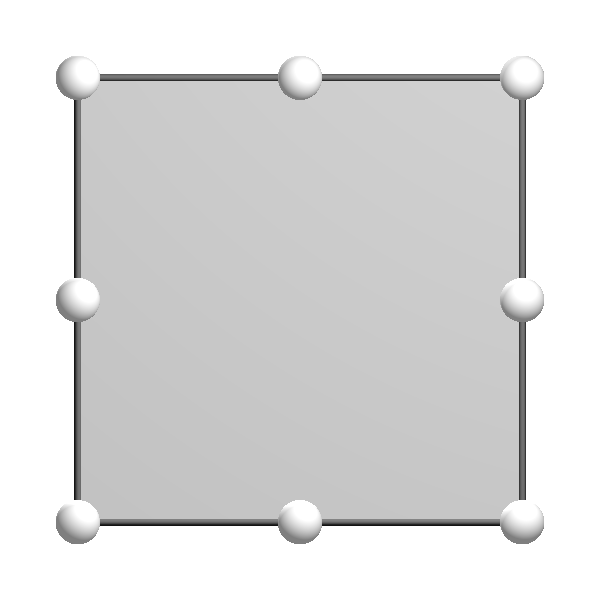
$\SS_{2}\times\SS_{2}$ ${\mathcal{P}}_{0}$ ${\mathcal{B}\mathcal{D}\mathcal{M}}_{1}$ ${\mathcal{P}}_{0}$ $\underbrace{\hskip 156.49014pt}_{\text{\normalsize Stokes}}$ $\underbrace{\hskip 156.49014pt}_{\text{\normalsize mixed Poisson}}$

Figure 4. Degrees of freedom used to construct the second elements.

This Stokes element is the one referred to as $Q^{(8)}_{2}$–$P_{0}$ in [17], for which it is easy to prove stability using the edge degrees of freedom. This is discussed in [17], where it is shown the inf-sup condition (S3) holds (on general quadrilateral meshes) for a variant of the element ($R^{(8)}_{2}$–$P_{0}$) which uses the same pressure space and a smaller velocity space. This of course implies the inf–sup condition with the larger velocity space. The $BDM_{1}$–$P_{0}$ element is a standard stable mixed finite element for the Poisson equation. Its stability on general quadrilateral meshes is shown, for instance, in [4]. Thus all the hypotheses of Theorems 1 and 2 are again met, and the choice $\Sigma_{h}=S_{h}\times S_{h}$, $V_{h}=U_{h}\times U_{h}$, and $Q_{h}$ give a stable element for elasticity.

5. $L^{2}$ estimates and rates of convergence

The rate of convergence that can be deduced from the quasioptimal error estimate (4) is limited by the approximation properties of the finite element space $\Sigma_{h}$ in the $H(\operatorname{div})$ norm. We can demonstrate higher rates of convergence by establishing a bound in the $L^{2}$ norm, as we do in this section.

In order to obtain an estimate in $L^{2}(\Omega,\mathbb{M})\times L^{2}(\Omega,\mathbb{R}^{2})\times L^{2}(\Omega)$, we impose a further condition:

• There exists a projection $\Pi_{h}$ from $H^{1}(\Omega,\mathbb{M})$ onto $\Sigma_{h}$ such that

  $$P_{V_{h}}\operatorname{div}\Pi_{h}\sigma=P_{V_{h}}\operatorname{div}\sigma.$$

Here $P_{V_{h}}:L^{2}(\Omega,\mathbb{R}^{2})\to V_{h}$ is the $L^{2}$-projection.

Theorem 3.

Suppose that conditions (S0) and (S5) are satified. Then

$$\lVert\sigma-\sigma_{h}\rVert_{L^{2}}+\lVert u-u_{h}\rVert_{L^{2}}+\lVert p-p_{h}\rVert_{L^{2}}\\ \leq C(\lVert\sigma-\Pi_{h}\sigma\rVert_{L^{2}}+\lVert u-P_{V_{h}}u\rVert_{L^{2}}+\lVert p-P_{Q_{h}}p\rVert_{L^{2}}).$$

Proof.

We decompose the error into the projected error

$$\eta_{h}=(\Pi_{h}\sigma-\sigma_{h},P_{V_{h}}u-u_{h},P_{Q_{h}}p-p_{h})\in Y_{h},$$

and the projection error

$$\bar{\eta}_{h}=(\sigma-\Pi_{h}\sigma,u-P_{V_{h}}u,p-P_{Q_{h}}p).$$

Making use of the triangle inequality, it suffices to show that $\lVert\eta_{h}\rVert_{L^{2}}\leq C\lVert\bar{\eta}_{h}\rVert$.

By the inf-sup condition (S0), there exists a non-zero $z=(\tau,v,q)\in Y_{h}$ such that

(16) $$B(\eta_{h},z)\geq c_{0}\lVert\eta_{h}\rVert_{Y}\lVert z\rVert_{Y}\geq c_{0}\lVert\eta_{h}\rVert_{L^{2}}\lVert z\rVert_{Y}.$$

Now, by Galerkin orthogonality,

(17) $$B(\eta_{h},z)=-B(\bar{\eta}_{h},z).$$

The quantity $B(\bar{\eta}_{h},z)$ is a sum of five terms according to the definition (2) of the bilinear form, but the fourth term, $(\operatorname{div}(\sigma-\Pi_{h}\sigma),v)$, vanishes, because of the assumption (S5). We then have

(18) $$B(\bar{\eta}_{h},z)\leq C\lVert\bar{\eta}_{h}\rVert_{L^{2}}\lVert z\rVert_{Y},$$

where $C$ depends only on an upper bound for $A$. Combining (16), (17), and (18), we conclude that $\lVert\eta_{h}\rVert_{L^{2}}\leq c_{0}^{-1}C\lVert\bar{\eta}_{h}\rVert_{L^{2}}$. ∎∎

We now give a simple criteria which makes it easy to verify that all finite element spaces introduced in Section 4 satisfy assumption (S5). See [4] for details on the verification.

Lemma 3.

Let $\hat{\Pi}$ be a bounded projection operator from $H^{1}(\hat{K},\mathbb{M})$ onto $\hat{\Sigma}$ such that

(19) $$\operatorname{div}\hat{\Pi}\hat{\sigma}=P_{\hat{V}}\operatorname{div}\hat{\sigma},\quad\forall\hat{\sigma}\in H^{1}(\hat{K},\mathbb{M}),$$

where $P_{\hat{V}}$ is the $L^{2}$-projection onto $\hat{V}$. Define $\Pi_{h}:H^{1}(\Omega,\mathbb{M})\to V_{h}$ by

$$\Pi_{h}\sigma|_{K}=P_{K}^{1}\hat{\Pi}(P_{K}^{1})^{-1}(\sigma|_{K}),\quad\forall K\in{\mathcal{T}}_{h}.$$

Then, we have that

$$P_{V_{h}}\operatorname{div}\Pi_{h}\sigma=P_{V_{h}}\operatorname{div}\sigma,\quad\forall\sigma\in H^{1}(\Omega,\mathbb{M}).$$

Proof.

Given $\sigma\in H^{1}(\Omega,\mathbb{M})$, we have $\hat{\sigma}:=(P_{K}^{1})^{-1}\left(\sigma|_{K}\right)\in H^{1}(\hat{K},\mathbb{M})$ for any $K\in\mathcal{T}_{h}$. For $v\in V_{h}$, we have $\hat{v}:=\left(P_{K}^{0}\right)^{-1}\left(v|_{K}\right)\in\hat{V}$ and by (7), (8) and (19), we have

$$(\operatorname{div}\Pi_{h}\sigma,v)_{L^{2}(K)} =(\operatorname{div}P_{K}^{1}\hat{\Pi}\hat{\sigma},P_{K}^{0}\hat{v})_{L^{2}(K)}=(P_{K}^{2}\operatorname{div}\hat{\Pi}\hat{\sigma},P_{K}^{0}\hat{v})_{L^{2}(K)}=(\operatorname{div}\hat{\Pi}\hat{\sigma},\hat{v})_{L^{2}(\hat{K})}$$

$$=(P_{\hat{V}}\operatorname{div}\hat{\sigma},\hat{v})_{L^{2}(\hat{K})}=(\operatorname{div}\hat{\sigma},\hat{v})_{L^{2}(\hat{K})}=(\operatorname{div}\sigma,v)_{L^{2}(K)}.$$

∎∎

5.1. Approximation properties on quadrilateral meshes

We now recall some results on the approximation rates achieved by finite element spaces on shape regular meshes of convex quadrilaterals. In [3] it is shown that if $X_{h}$ is a finite element space of scalar functions derived from shape function spaces $X_{K}$ which are themselves obtained from a reference shape function space $\hat{X}$ via the transformation $P_{K}^{0}$, then $X_{h}$ achieves approximation order $r+1$ in the $L^{2}$ norm if and only if ${\mathcal{Q}}_{r}\subset\hat{X}$. In [4], it shown that if $X_{h}$ is a finite element space of vector fields derived from shape function spaces $X_{K}$ defined from a reference space $\hat{X}$ via the Piola transform $P_{K}^{1}$, then a necessary and sufficient condition for order $r+1$ approximation in the $L^{2}$ norm is that $\mathcal{U}_{r}\subset\hat{X}$ while the condition for order $r+1$ approximation of $\operatorname{div}u$ in the $L^{2}$ is $\mathcal{R}_{r}\subset\operatorname{div}\hat{X}$. Here $\mathcal{U}_{r}$ is the subspace of codimension $1$ of ${\mathcal{R}\mathcal{T}}_{r+1}$ defined as the span of the vector fields

$$(\hat{x}_{1}^{i}\hat{x}_{2}^{j},0),\ (0,\hat{x}_{1}^{j}\hat{x}_{2}^{i}),\quad 0\leq i\leq r+1,\ 0\leq j\leq r,$$

except that the two vector fields $(\hat{x}_{1}^{r+1}\hat{x}_{2}^{r},0)$ and $(0,\hat{x}_{1}^{r}\hat{x}_{2}^{r+1})$ are replaced by the single vector field $(\hat{x}_{1}^{r+1}\hat{x}_{1}^{r},-\hat{x}_{1}^{r}\hat{x}_{1}^{r+1})$. The space $\mathcal{R}_{r}$ is the subspace of codimension $1$ of ${\mathcal{Q}}_{r+1}$ spanned by all its monomials except $\hat{x}_{1}^{r+1}\hat{x}_{2}^{r+1}$.

5.2. Rates of convergence of the proposed elements

Our first choice of finite element spaces is built from the reference space ${\mathcal{R}\mathcal{T}}_{2}$ transformed by $P_{K}^{1}$, the space $Q_{1}$ transformed by ${\mathcal{P}}_{K}^{0}$, and the space $P_{1}$, not subject to a transformation, as depicted in Figure 2. It follows that each of these spaces achieves quadratic convergence in $L^{2}$. In light of Theorem 3, the finite element solution converges quadratically in $L^{2}$ for all variables if the solution is smooth. Concerning approximation of the divergence, we have $\mathcal{R}_{0}\subset Q_{1}=\operatorname{div}{\mathcal{R}\mathcal{T}}_{2}$, but $\mathcal{R}_{1}\nsubseteq\operatorname{div}{\mathcal{R}\mathcal{T}}_{2}$, so the approximation error in $H(\operatorname{div})$ is only first order (and so the finite element method converges with first order in $H(\operatorname{div})$ by (4). Similarly, the higher order methods of this family, described in Section 4.2, achieve order $r$ convergence in $L^{2}$ for all variables, but in $H(\operatorname{div})$ the convergence order for the stress is reduced to $r-1$. Of course on meshes in which all the elements are square, or, more generally, parallelograms, the rate of convergence in $H(\operatorname{div})$ is $r$.

Similar reasoning, applied to the simple choice of elements described in Section 4.3 and illustrated in Figure 3, establishes linear convergence for all variables in $L^{2}$. However, since $\mathcal{R}_{0}\nsubseteq{\mathcal{P}}_{1}=\operatorname{div}{\mathcal{B}\mathcal{D}\mathcal{M}}_{1}$, we do not expect any convergence in $H(\operatorname{div})$ on general quadrilateral meshes.

6. Numerical results

In this section, we present simple numerical results which illustrates the error estimates just obtained. We take the domain to be the unit square and consider two sequences of meshes, the first using uniform meshes into subsquares, and the second consisting of meshes in which every element is congruent to a fixed trapezoid, as illustrated in Figure 5. The trapezoidal mesh sequence was introduced in [3] to study finite element approximation on quadrilateral meshes. For the test problem we take the elasticity system with homogeneous Dirichlet boundary conditions and the exact solution

$$u_{1}=\cos(\pi x)\sin(2\pi y),\quad u_{2}=\sin(\pi x)\cos(\pi y).$$

The body force $f$ is then determined using the values $\lambda=123$ and $\mu=79.3$ for the Lamé coefficients.

 

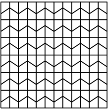
Figure 5. Square and trapezoidal meshes.

In Table 1, we show errors and convergence rates in the $L^{2}$ norm for $\sigma$, $\operatorname{div}\sigma$, $u$ and $p$, using the elements of Section 4.1. As expected all three variables converge quadratically in $L^{2}$, while $\operatorname{div}\sigma$ converges only linearly with trapezoidal meshes, and quadratically for square meshes. Table 2 illustrates the same quantities for the simple stable choice of elasticity elements of Section 4.3, showing the expected linear convergence, which reduces to no convergence for the divergence computed with trapezoidal meshes.

Table 1. Convergence results for the elements of Section 4.1 (illustrated in Figure 2).

Square meshes
	$\|\sigma-\sigma_{h}\|_{L^{2}(\Omega)}$			$\|\operatorname{div}(\sigma-\sigma_{h})\|_{L^{2}(\Omega)}$
$h$	error	$\quad\%$	order	error	$\quad\%$	order
$1/2$	$3.06$e$+$$2$	$31.8$		$1.83$e$+$$3$	$35.9$
$1/4$	$6.64$e$+$$1$	$\hphantom{0}6.91$	$2.2$	$4.19$e$+$$2$	$\hphantom{0}8.21$	$2.1$
$1/8$	$1.59$e$+$$1$	$\hphantom{0}1.65$	$2.1$	$1.07$e$+$$2$	$\hphantom{0}2.10$	$2.0$
$1/16$	$3.88$e$+$$0$	$\hphantom{0}0.403$	$2.0$	$2.70$e$+$$1$	$\hphantom{0}0.529$	$2.0$
$1/32$	$9.61$e$-$$1$	$\hphantom{0}0.0998$	$2.0$	$6.77$e$+$$0$	$\hphantom{0}0.132$	$2.0$
$1/64$	$2.39$e$-$$1$	$\hphantom{0}0.0248$	$2.0$	$1.69$e$+$$0$	$\hphantom{0}0.0331$	$2.0$
$1/128$	$5.98$e$-$$2$	$\hphantom{0}0.00621$	$2.0$	$4.23$e$-$$1$	$\hphantom{0}0.00828$	$2.0$
	$\|u-u_{h}\|_{L^{2}(\Omega)}$			$\|p-p_{h}\|_{L^{2}(\Omega)}$
$h$	error	$\quad\%$	order	error	$\quad\%$	order
$1/2$	$2.33$e$-$$1$	$33.0$		$7.28$e$-$$1$	$41.5$
$1/4$	$4.87$e$-$$2$	$\hphantom{0}6.89$	$2.3$	$2.17$e$-$$1$	$12.4$	$1.7$
$1/8$	$1.24$e$-$$2$	$\hphantom{0}1.76$	$2.0$	$5.60$e$-$$2$	$\hphantom{0}3.19$	$2.0$
$1/16$	$3.12$e$-$$3$	$\hphantom{0}0.442$	$2.0$	$1.40$e$-$$2$	$\hphantom{0}0.800$	$2.0$
$1/32$	$7.82$e$-$$4$	$\hphantom{0}0.110$	$2.0$	$3.51$e$-$$3$	$\hphantom{0}0.200$	$2.0$
$1/64$	$1.95$e$-$$4$	$\hphantom{0}0.0276$	$2.0$	$8.78$e$-$$4$	$\hphantom{0}0.0500$	$2.0$
$1/128$	$4.89$e$-$$5$	$\hphantom{0}0.00691$	$2.0$	$2.19$e$-$$4$	$\hphantom{0}0.0125$	$2.0$
Trapezoidal meshes
	$\|\sigma-\sigma_{h}\|_{L^{2}(\Omega)}$			$\|\operatorname{div}(\sigma-\sigma_{h})\|_{L^{2}(\Omega)}$
$h$	error	$\quad\%$	order	error	$\quad\%$	order
$1/2$	$3.35$e$+$$2$	$34.8$		$2.06$e$+$$3$	$40.4$
$1/4$	$8.93$e$+$$1$	$\hphantom{0}9.29$	$1.9$	$5.95$e$+$$2$	$11.6$	$1.8$
$1/8$	$2.11$e$+$$1$	$\hphantom{0}2.19$	$2.0$	$1.84$e$+$$2$	$\hphantom{0}3.60$	$1.6$
$1/16$	$5.24$e$+$$0$	$\hphantom{0}0.560$	$2.0$	$7.14$e$+$$1$	$\hphantom{0}1.40$	$1.3$
$1/32$	$1.30$e$+$$0$	$\hphantom{0}0.135$	$2.0$	$3.25$e$+$$1$	$\hphantom{0}0.636$	$1.1$
$1/64$	$3.26$e$-$$1$	$\hphantom{0}0.0339$	$2.0$	$1.58$e$+$$1$	$\hphantom{0}0.310$	$1.0$
$1/128$	$8.16$e$-$$2$	$\hphantom{0}0.00847$	$2.0$	$7.87$e$+$$0$	$\hphantom{0}0.154$	$1.0$
	$\|u-u_{h}\|_{L^{2}(\Omega)}$			$\|p-p_{h}\|_{L^{2}(\Omega)}$
$h$	error	$\quad\%$	order	error	$\quad\%$	order
$1/2$	$2.59$e$-$$1$	$36.7$		$7.34$e$-$$1$	$41.8$
$1/4$	$6.57$e$-$$2$	$\hphantom{0}9.30$	$1.9$	$2.61$e$-$$1$	$14.9$	$1.4$
$1/8$	$1.57$e$-$$2$	$\hphantom{0}2.23$	$2.0$	$7.12$e$-$$2$	$\hphantom{0}4.06$	$1.8$
$1/16$	$3.96$e$-$$3$	$\hphantom{0}0.560$	$1.9$	$1.79$e$-$$2$	$\hphantom{0}1.02$	$1.9$
$1/32$	$9.93$e$-$$4$	$\hphantom{0}0.140$	$2.0$	$4.49$e$-$$3$	$\hphantom{0}0.256$	$2.0$
$1/64$	$2.48$e$-$$4$	$\hphantom{0}0.0351$	$2.0$	$1.12$e$-$$3$	$\hphantom{0}0.064$	$2.0$
$1/128$	$6.20$e$-$$5$	$\hphantom{0}0.00878$	$2.0$	$2.81$e$-$$4$	$\hphantom{0}0.0160$	$2.0$

Table 2. Convergence results for the elements of Section 4.3 (illustrated in Figure 3).

Square meshes
	$\|\sigma-\sigma_{h}\|_{L^{2}(\Omega)}$			$\|\operatorname{div}(\sigma-\sigma_{h})\|_{L^{2}(\Omega)}$
$h$	error	$\quad\%$	order	error	$\quad\%$	order
$1/2$	$6.20$e$+$$2$	$64.5$		$3.40$e$+$$3$	$66.5$
$1/4$	$2.51$e$+$$2$	$26.2$	$1.3$	$2.28$e$+$$3$	$44.8$	$0.5$
$1/8$	$1.09$e$+$$2$	$11.4$	$1.2$	$1.18$e$+$$3$	$23.3$	$0.9$
$1/16$	$5.23$e$+$$1$	$\hphantom{0}5.43$	$1.1$	$6.00$e$+$$2$	$11.7$	$1.0$
$1/32$	$2.58$e$+$$1$	$\hphantom{0}2.68$	$1.0$	$3.01$e$+$$2$	$\hphantom{0}5.89$	$1.0$
$1/64$	$1.28$e$+$$1$	$\hphantom{0}1.34$	$1.0$	$1.50$e$+$$2$	$\hphantom{0}2.95$	$1.0$
$1/128$	$6.42$e$+$$0$	$\hphantom{0}0.667$	$1.0$	$7.53$e$+$$1$	$\hphantom{0}1.47$	$1.0$
	$\|u-u_{h}\|_{L^{2}(\Omega)}$			$\|p-p_{h}\|_{L^{2}(\Omega)}$
$h$	error	$\quad\%$	order	error	$\quad\%$	order
$1/2$	$4.29$e$-$$1$	$60.7$		$1.63$e$+$$0$	$93.4$
$1/4$	$2.90$e$-$$1$	$41.1$	$0.5$	$7.97$e$-$$1$	$45.4$	$1.0$
$1/8$	$1.49$e$-$$1$	$21.1$	$1.0$	$4.13$e$-$$1$	$23.6$	$0.9$
$1/16$	$7.48$e$-$$2$	$10.6$	$1.0$	$2.08$e$-$$1$	$11.9$	$1.0$
$1/32$	$3.74$e$-$$2$	$\hphantom{0}5.30$	$1.0$	$1.04$e$-$$1$	$\hphantom{0}5.94$	$1.0$
$1/64$	$1.87$e$-$$2$	$\hphantom{0}2.65$	$1.0$	$5.21$e$-$$2$	$\hphantom{0}2.97$	$1.0$
$1/128$	$9.37$e$-$$3$	$\hphantom{0}1.32$	$1.0$	$2.61$e$-$$2$	$\hphantom{0}1.49$	$1.0$
Trapezoidal meshes
	$\|\sigma-\sigma_{h}\|_{L^{2}(\Omega)}$			$\|\operatorname{div}(\sigma-\sigma_{h})\|_{L^{2}(\Omega)}$
$h$	error	$\quad\%$	order	error	$\quad\%$	order
$1/2$	$6.67$e$+$$2$	$69.3$		$3.70$e$+$$3$	$72.4$
$1/4$	$2.90$e$+$$2$	$30.2$	$1.1$	$2.58$e$+$$3$	$50.6$	$0.52$
$1/8$	$1.22$e$+$$2$	$12.7$	$1.2$	$1.59$e$+$$3$	$31.3$	$0.69$
$1/16$	$5.77$e$+$$1$	$\hphantom{0}6.00$	$1.0$	$1.19$e$+$$3$	$23.4$	$0.42$
$1/32$	$2.84$e$+$$1$	$\hphantom{0}2.95$	$1.0$	$1.06$e$+$$3$	$20.8$	$0.16$
$1/64$	$1.41$e$+$$1$	$\hphantom{0}1.46$	$1.0$	$1.03$e$+$$3$	$20.2$	$0.05$
$1/128$	$7.03$e$+$$0$	$\hphantom{0}0.731$	$1.0$	$1.02$e$+$$3$	$20.0$	$0.01$
	$\|u-u_{h}\|_{L^{2}(\Omega)}$			$\|p-p_{h}\|_{L^{2}(\Omega)}$
$h$	error	$\quad\%$	order	error	$\quad\%$	order
$1/2$	$4.72$e$-$$1$	$66.8$		$1.70$e$+$$0$	$97.0$
$1/4$	$2.97$e$-$$1$	$42.1$	$0.6$	$9.05$e$-$$1$	$51.6$	$0.9$
$1/8$	$1.60$e$-$$1$	$22.6$	$0.8$	$4.46$e$-$$1$	$25.4$	$1.0$
$1/16$	$8.05$e$-$$2$	$11.4$	$1.0$	$2.25$e$-$$1$	$12.8$	$0.9$
$1/32$	$4.03$e$-$$2$	$\hphantom{0}5.70$	$1.0$	$1.12$e$-$$1$	$\hphantom{0}6.42$	$1.0$
$1/64$	$2.01$e$-$$2$	$\hphantom{0}2.85$	$1.0$	$5.64$e$-$$2$	$\hphantom{0}3.21$	$1.0$
$1/128$	$1.00$e$-$$2$	$\hphantom{0}1.43$	$1.0$	$2.82$e$-$$2$	$\hphantom{0}1.61$	$1.0$

In Figure 6, we show numerical evidence of the locking-free property of the BDM type elements of Section 4.3 (illustrated in Figure 3) on trapezoidal meshes. The exact solution is the same as above and the Young’s modulus $E$ is taken as $1000$. The two figures show the convergence history of the stress and displacement as a function of the total number of degrees of freedom for the stress, the displacement and the rotation. We used various values of the Poisson ratio $\nu$ close to the limiting value of $0.5$. Recall that

$$\lambda=\frac{E\nu}{(1+\nu)(1-2\nu)}.$$

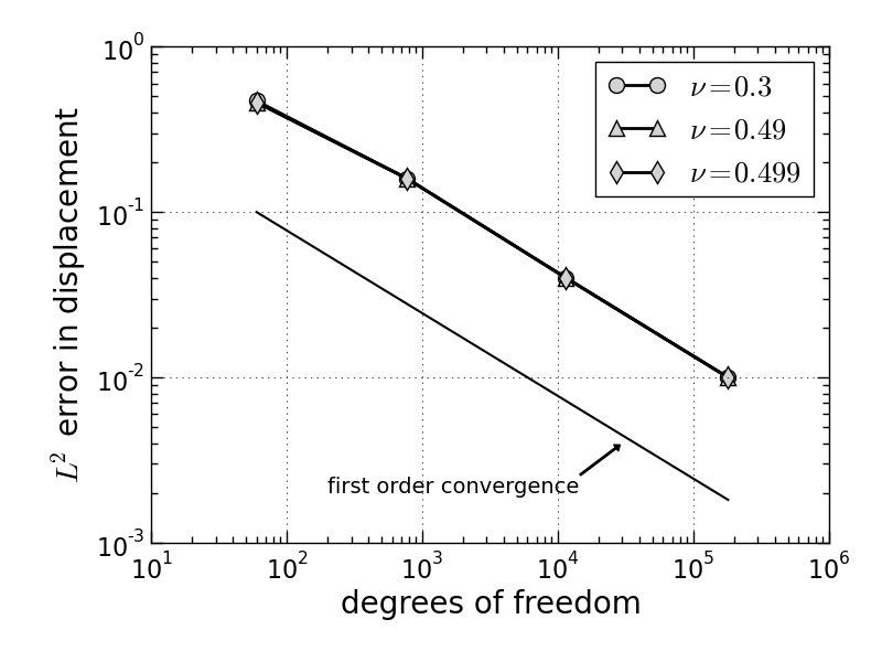
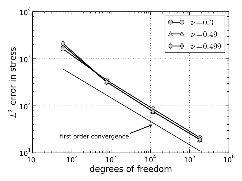
Figure 6. Error of the first order method for several values of the Poisson ratio, displacement on left, stress on the right. The curves nearly coincide, illustrating the absence of locking.

References

- [1] Mohamed Amara and Jean-Marie Thomas, Equilibrium finite elements for the linear elastic problem, Numer. Math. 33 (1979), 367–383.
- [2] Douglas N. Arnold and Gerard Awanou, Rectangular mixed finite elements for elasticity, Math. Models Methods Appl. Sci. 15 (2005), no. 9, 1417–1429.
- [3] Douglas N. Arnold, Daniele Boffi, and Richard S. Falk, Approximation by quadrilateral finite elements, Math. Comp. 71 (2002), no. 239, 909–922 (electronic).
- [4] by same author, Quadrilateral finite elements, SIAM J. Numer. Anal. 42 (2005), no. 6, 2429–2451.
- [5] Douglas N. Arnold, Franco Brezzi, and Jim Douglas, Jr., PEERS: a new mixed finite element for plane elasticity, Japan J. Appl. Math. 1 (1984), no. 2, 347–367.
- [6] Douglas N. Arnold, Richard S. Falk, and Ragnar Winther, Differential complexes and stability of finite element methods II: The elasticity complex, Compatible Spatial Discretizations (D. Arnold, P. Bochev, R. Lehoucq, R. Nicolaides, and M. Shaskov, eds.), IMA Vol. Math. Appl., vol. 142, Springer, Berlin, 2006, pp. 47–68.
- [7] by same author, Finite element exterior calculus, homological techniques, and applications, Acta Numer. 15 (2006), 1–155.
- [8] by same author, Mixed finite element methods for linear elasticity with weakly imposed symmetry, Math. Comput. 76 (2007), 1699–1723.
- [9] Douglas N. Arnold and Ragnar Winther, Mixed finite elements for elasticity, Numer. Math. 92 (2002), 401–419. MR MR1930384 (2003i:65103)
- [10] Gerard Awanou, Rectangular mixed elements for elasticity with weakly imposed symmetry condition, Adv. Comput. Math. 38 (2013), no. 2, 351–367.
- [11] Daniele Boffi, Franco Brezzi, and Michel Fortin, Reduced symmetry elements in linear elasticity, Commun. Pure Appl. Anal. 8 (2009), no. 1, 95–121.
- [12] by same author, Mixed finite element methods and applications, Springer Series in Computational Mathematics, vol. 44, Springer, Heidelberg, 2013. MR 3097958
- [13] Franco Brezzi, On the existence, uniqueness and approximation of saddle-point problems arising from Lagrangian multipliers, Rev. Française Automat. Informat. Recherche Opérationnelle Sér. Rouge 8 (1974), 129–151.
- [14] Bernardo Cockburn, Jayadeep Gopalakrishnan, and Johnny Guzmán, A new elasticity element made for enforcing weak stress symmetry, Math. Comp. 79 (2010), no. 271, 1331–1349.
- [15] Richard S. Falk, Finite element methods for linear elasticity, Mixed finite elements, compatibility conditions, and applications (Daniele Boffi and Lucia Gastaldi, eds.), Lecture Notes in Mathematics, vol. 1939, Springer-Verlag, Berlin, 2008, Lectures given at the C.I.M.E. Summer School held in Cetraro, June 26–July 1, 2006.
- [16] Mohamed Farhloul and Michel Fortin, Dual hybrid methods for the elasticity and the Stokes problems: a unified approach, Numer. Math. 76 (1997), 419–440.
- [17] Michel Fortin, Old and new finite elements for incompressible flows, Internat. J. Numer. Methods Fluids 1 (1981), no. 4, 347–364.
- [18] Badouin M. Fraeijs de Veubeke, Displacement and equilibrium models in the finite element method, Stress Analysis (O. C. Zienkiewicz and G. S. Holister, eds.), Wiley, New York, 1965, pp. 145–197.
- [19] Vivette Girault and Pierre-Arnaud Raviart, Finite element methods for Navier-Stokes equations, Springer Series in Computational Mathematics, vol. 5, Springer, Berlin, 1986.
- [20] Jayadeep Gopalakrishnan and Johnny Guzmán, A second elasticity element using the matrix bubble, IMA J. Numer. Anal. 32 (2012), no. 1, 352–372.
- [21] C. Johnson and B. Mercier, Some equilibrium finite element methods for two-dimensional elasticity problems, Numer. Math. 30 (1978), no. 1, 103–116.
- [22] Mary E. Morley, A family of mixed finite elements for linear elasticity, Numer. Math. 55 (1989), no. 6, 633–666.
- [23] Rolf Stenberg, On the construction of optimal mixed finite element methods for the linear elasticity problem, Numer. Math. 48 (1986), no. 4, 447–462.
- [24] by same author, A family of mixed finite elements for the elasticity problem, Numer. Math. 53 (1988), no. 5, 513–538.
- [25] by same author, Two low-order mixed methods for the elasticity problem, The mathematics of finite elements and applications, VI (Uxbridge, 1987), Academic Press, London, 1988, pp. 271–280.
- [26] V. B. Watwood, Jr. and B. J. Hartz, An equilibrium stress field model for finite element solution of two-dimensional elastostatic problems, Internat. J. Solids Structures 4 (1968), 857–873.