Opinion dynamics model with weighted influence: Exit probability and dynamics

Abstract

We introduce a stochastic model of binary opinion dynamics in which the opinions are determined by the size of the neighbouring domains. The exit probability here shows a step function behaviour indicating the existence of a separatrix distinguishing two different regions of basin of attraction. This behaviour, in one dimension, is in contrast to other well known opinion dynamics models where no such behaviour has been observed so far. The coarsening study of the model also yields novel exponent values. A lower value of persistence exponent is obtained in the present model, which involves stochastic dynamics, when compared to that in a similar type of model with deterministic dynamics. This apparently counter-intuitive result is justified using further analysis. Based on these results it is concluded that the proposed model belongs to a unique dynamical class.

I Introduction

Nonequilibrium dynamics has been a topic of intensive research over the last few decades. The fact that models displaying identical equilibrium behaviour can be differentiated on the basis of critical relaxation, coarsening and persistence behaviour, has enhanced the interest in this field. Traditionally critical and off critical dynamical behaviour were studied for magnetic systems with different dynamical rules and constraints Hoha ; bray . More recently, physicists have been able to construct dynamical models in problems which are interdisciplinary in nature, where one can investigate how such models can be classified into different dynamical classes.

One very popular interdisciplinary topic is opinion dynamics, where a number of models stau ; qvote ; cast_sat ; kszjsz have been proposed and studied by physicists, many of which can also be regarded as spin models. The dynamical rules in all the well studied opinion dynamics models with binary opinions ($\pm 1$) in one dimension lead to the consensus state. The question whether the intrinsic dynamics for ordering are equivalent has been asked in context of the generalised $q$ state voter model qvote , generalised Glauber models cast_sat and Sznajd models kszjsz ; slanina . One of the quantities which is computed to resolve this important question is the exit probability (EP) which denotes the probability $f_{up}(x)$ that one ends up in a configuration with all opinions equal to 1 starting from $x$ fraction of opinions equal to 1. EP has been shown to be identical cast_sat in the generalised Glauber model and the Sznajd model; the latter was originally claimed to have a different dynamical scenario. In the voter model (or Ising Glauber model) in one dimension, $f_{up}(x)$ is simply equal to $x$, corresponding to the conservation in the dynamics cast_review . In the nonlinear voter model, long ranged Sznajd model and long ranged Glauber model, it is a nonlinear continuous function of $x$ cast_sat ; slanina ; lamb-redner2008 . In all these cases, the results are also independent of finite system sizes indicating there is no scaling behaviour. The claim that the exit probability for Sznajd model is a continuous function has been however questioned in galmart . But analytical and numerical study of $q$ state nonlinear voter model (Sznajd model corresponds to nonlinear voter model with $q=2$) show that EP is a continuous function of $x$ przy . Interestingly, the mean field result was shown to be exact in the nonlinear $q$ voter model which includes the Sznajd model and independent of the range cast_sat ; przy . On the other hand, in two dimensions or on networks, the exit probability shows a step function behaviour in many models which has been interpreted as a phase transition. $f_{up}(x)$ also shows finite size dependence in that case staufferetal ; croki . However, strictly speaking, one should interpret this as the existence of a separatrix between two different regions of basin of attraction - where the attractors are the states with all opinions equal to $1$ or $-1$.

In this paper, we have proposed a model (the weighted influence model, WI model hereafter) which shows completely different behaviour as the EP has a step function behaviour even in one dimension. The result also shows clear deviation from mean field theory, although the latter provides a reasonable first order estimate. The model includes one parameter which allows one to obtain a relevant “phase diagram” and also show the presence of universal behaviour.

Apart from studying the exit probability, we also investigate the dynamical behaviour of the WI model by studying the density of domain walls $D(t)$ and persistence probability ${\cal{P}}(t)$ as functions of time $t$ starting from an initial disordered state. The latter is the probability that a spin has not flipped till time $t$ deribray . It is known that in conventional coarsening processes, $D(t)\propto t^{-1/z}$ and ${\cal{P}}(t)$ shows a scaling behaviour ${\cal{P}}(t)\propto t^{-\theta}$ in many systems bray where $z$ and $\theta$ are the dynamic (growth) and persistence exponents respectively. By calculating $z$ and $\theta$, the dynamical class of the model can be identified and compared to models for which these exponents are known, for example, for the zero temperature Ising model in one dimension, $z=2$ and $\theta=0.375$ are exactly known results.

The rest of the paper is arranged as follows: Sec. II describes the model. Sec. III discusses the mean field theory in the context of the present work. Numerical results obtained from extensive simulations are presented in Sec. IV. Dynamical properties of the model are given in Sec. V and finally in Sec. VI, concluding remarks are made.

II Description of the model

The WI model is a stochastic model with opinions taking values $\pm 1$, and there is a bias towards one type of opinion controlled by a relative weight factor. It cannot be true that an initial majority always wins (in that case the same candidate/party will go on winning elections every time) elections and a huge majority of people may give up to an initial minority view minor ; galam_minority . The relative weight factor included in the model takes care of this idea. This weight factor represents the relative strength that may arise due to monetary factors, local factors, muscle power, larger accountability, traditional, religious or cultural influence, recent incidents which has a great impact on the population etc. The model is described in the following way. Let there be two groups of people with opposing opinion in the immediate spatial neighbourhood of an individual. Under the influence of these two groups, she/he will be under pressure to follow one group. The pressure is proportional to the size of the group. Denoting the two neighbouring opposing group sizes as $S_{1}$ and $S_{-1}$ for opinion = $\pm 1$ respectively, an individual takes up opinion $1$ with probability

$$P_{1}=\frac{S_{1}}{S_{1}+\delta S_{-1}},$$ (1)

where $\delta$ is the relative influencing ability of the two groups and can vary from zero to $\infty$. Probability to take opinion value $-1$ is $P_{-1}=1-P_{1}.$ The model is considered in one dimension. In case an individual with opinion $1$ ($-1$) has both nearest neighbours with opinion $-1$ ($+1$), her opinion will change deterministically. The unweighted model corresponds to $\delta=1$ foot .

In this model, the dynamics is completely stochastic. A quasi-deterministic model in which the neighbouring domain sizes determine the state of a spin had been proposed earlier (BS model hereafter) pssb1 . The BS model takes into consideration the sizes of neighbouring domains in the dynamics and the larger neighbouring domain always dictates the opinion, irrespective of its size. Only in the case when the neighbouring domains are of equal size (which occurs rarely) is the dynamical rule stochastic. In the BS model, $z\simeq 1$ and $\theta\simeq 0.235$ (both the exponents are different from the Ising model). We find some interesting effects of the nature of the stochasticity in the WI model, especially regarding the persistence behaviour, which is revealed when compared to the BS model and Ising model dynamical results.

Regarding the binary opinion values as Ising spin states (up/down), the absorbing states are the all up/all down states in the WI model. Probability of attaining these consensus states however depends on the value of $\delta$ instead of being simply 1/2 (as in the Ising or voter model) even when one starts from a completely random initial configuration ($x=1/2$). In the limit $\delta=0$, all spins will be up as $P_{1}=1$ for any initial value of $x$ while for $\delta\to\infty$, the final state will be all down for any value of $x\neq 1$. Thus the threshold values $x_{c}$ for which the final state will be all up is zero for $\delta=0$ and 1 for $\delta\to\infty$. The exit probability is trivially a step function in these extreme limits. The question is what happens for other values of $\delta$, including $\delta=1$.

III Mean field theory

The dynamics can be studied in terms of the motion of domain walls as only the spins adjacent to domain walls can flip. In a Glauber like process, one considers the flipping of a random spin in time $\Delta t$ with the time unit being such that $\Delta tL=1$, where $L$ is the total number of spins. Initially, there will be many domains of size one, but they will quickly vanish as it is a deterministic process. Assuming no domain of size one remains in the system and using a mean field approximation, one can write down a microscopic equation for the (average) fraction of up spins at time $t+\Delta t$ given that there was a fraction $x$ at $t$. It may be noted that in this approximation, the fluctuations in the flipping probabilities $P_{1}$ and $P_{-1}$ can be ignored and they can be taken to be site-independent. The equation for $x(t+\Delta t)$ is then given by

$$x(t+\Delta t) = r(t)[(x(t)-1/L)P_{-1}+x(t)P_{1}]$$ (2)

$$+r(t)[(x(t)+1/L)P_{1}+x(t)P_{-1}]$$

$$+(1-2r(t))x(t).$$

Here $r(t)$ is the density of domain walls, $r(t)\leq 1/2$ when domains have length at least 2. $P_{1},P_{-1}$ are also in general time dependent. The first two terms on the right hand side correspond to cases where the up and down spin at the boundary are chosen for flipping respectively while the last term is for the case when a spin within a domain is selected ($x$ remains same in the last case obviously). Thus one gets

$$\frac{dx}{dt}=r(t)[P_{1}-P_{-1}].$$ (3)

This equation cannot be solved without knowing the dynamical equation for $r(t)$ which is again expected to involve $x(t)$ in a complicated manner. However, the fixed points of the equation, in which we are actually interested, are easily obtained; a trivial fixed point $r(t)=0$ and the other one is $[P_{1}-P_{-1}]=0$. For the Ising or voter model, $P_{1}$ is equal to $P_{-1}$ which corresponds to the result that $dx/dt=0$ independent of $x$. This leads to the known result that the exit probability is simply equal to $x$. All points are fixed points here. In case one gets a single fixed point $x_{c}$ from Eq. (3), it will indicate the existence of the step function like behaviour associated with the exit probability. The mean field approximation of course neglects all correlations and fluctuations. In the WI model, $P_{-1}$ and $P_{1}$ in mean field approximation can be estimated by taking $S_{1}$ and $S_{-1}$ proportional to $x$ and $(1-x)$ respectively (at the fixed point) in Eq. (1). There is no reason to take the constant of proportionality to be different (i.e. there is no bias to either type of domain) such that $P_{1}=x/[x+\delta(1-x)]$ and we get

$$x_{c}=\delta/(1+\delta).$$ (4)

Although the mean field result involves many assumptions it is tempting to accept this result as it coincides with the limiting results that $x_{c}=0$ for $\delta=0$, $x_{c}=1.0$ for $\delta\to\infty$. The mean field result also predicts $x_{c}=1/2$ for $\delta=1$. $\delta=1$ corresponds to the model with unweighted influence, and here if one starts with $x=1/2$ the system will go to $+1$ state with $50\%$ probability (by the argument of symmetry). If there is any initial bias ($x\neq 1/2$) in the system then it will win at the end. EP will be zero for $x<1/2$ and equal to 1 for $x>1/2$. Hence one expects that at $\delta=1$, $x_{c}=1/2$ as given by (4).

Having obtained the evidence of a single value of $x_{c}$ from mean field approximation, our next job is to find out numerically whether there exists a separatrix and and whether finite size effects exist. Also, the deviation from mean field theory, if any, will be investigated in the following section.

IV Exit probability: numerical results

We calculate the exit probability $f_{up}$ for system sizes ranging from $L=5000$ to $L=50000$ and repeat the simulations for over at least $3000$ configurations for each system size. $f_{up}$ against initial concentration $x$ is shown in Fig. 1 for two values of $\delta$. It indeed shows a sharp rise close to a value of $x\simeq x_{c}$, henceforth called the separatrix point. The shape of the exit probability $f_{up}$ plotted against $x$ immediately shows that it is nonlinear, moreover, $f_{up}(x)$ curves show strong system size dependence and intersect at a single point $x_{c}$ for different values of $L$. The behaviour of EP indicates that it shows a step function behaviour in the thermodynamic limit. Finite size scaling analysis can be made using the scaling form (when $\delta$ is constant):

$$f_{up}(x,L)=f_{1}\left(\frac{(x-x_{c})}{x_{c}}{L^{1/\nu}}\right)$$ (5)

where $f_{1}(y)\to 0$ for $y<<0$ and equal to 1 for $y>>0$ (i.e., a step function in the thermodynamic limit). $f^{c}_{up}$ gives the the value of EP at the separatrix point. The data collapse, shown in Fig. 1, takes place with $\nu=2.50\pm 0.02$ for all values of $\delta$.

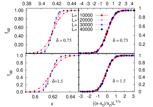
Figure 1: (Color online) The data for the exit probability against initial concentration $x$ (left panel) and the data collapse (right panel) using $\nu=2.50\pm 0.02$ (Eq. (5)) for different system sizes are shown.

For fixed $x$, the finite size scaling form for exit probability can be written as:

$$f_{up}(\delta,L)=f_{2}\left(\frac{(\delta-\delta_{c})}{\delta_{c}}{L^{1/\nu}}\right).$$ (6)

where $f_{2}(y)\to 0$ for $y>>0$, equal to 1 for $y<<0$. Both the scaling forms (Eqs (5) and (6)) give $\nu=2.50\pm 0.02$ independent of the exact location of the separatrix point. $x_{c}$ as a function of $\delta$ denotes the trajectory of the separatrix point as $\delta$ is varied and for convenience we call it the “phase boundary”. So one can conclude that universal behaviour exists along the entire phase boundary.

Estimating $x_{c}$ for different values of $\delta$, we plot the phase boundary in Fig. 3.

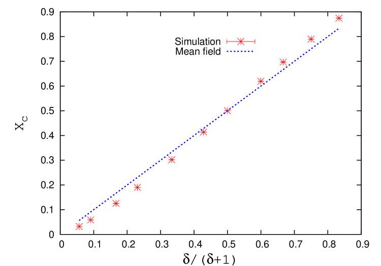
Figure 2: (Color online) The values of $x_{c}$ obtained by simulations and the mean field theory result (dashed line, Eq. (4) are compared. There is appreciable difference away from $\delta=1$; the difference vanishes as $\delta\to 0$ and $\delta\to\infty$.

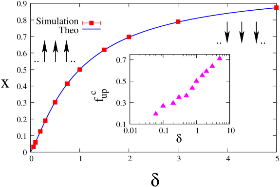
Figure 3: (Color online) Main plot: The phase boundary in the $x-\delta$ plane obtained from simulation and its theoretical fitting (Eq. (7)) separating the all up and all down phases. Inset shows variation of $f^{c}_{up}$ with $\delta$.

The phase boundary is not exactly given by the mean field estimate (4) but shows systematic deviation from this equation (except at $\delta=0,1.0$ and $\delta\to\infty$) as shown in Fig. 2. There is a systematic difference from the mean field results away from $\delta=1$ which vanishes at $\delta=0$ and also as $\delta\to\infty$. However, the difference is mostly less than ten percent for other values of $\delta$ and therefore the mean field result can be taken as a first order estimate. In principle, one may consider an expression of $x_{c}$ given by a polynomial in $\delta/(1+\delta)$ as obviously it deviates from a simple linear form. However, introducing only a second order term is not sufficient and we therefore attempt to fit the numerically obtained values of $x_{c}$ accurately by a single correction term, the form of which is conjectured by the known values of $x_{c}$ at $\delta=0,1$ and $\delta\to\infty$. We assume the following form for $x_{c}$:

$$x_{c}=\delta/(\delta+1)+a\delta(\delta-1)/(\delta+b)^{c}.$$ (7)

Here $\delta(\delta-1)$ in the correction term (second term on right hand side of Eq. (7)) takes care that the term vanishes for $\delta=0,1$. If one compares the numerical data with the mean field result (Fig. 2), the former gives larger values of $x_{c}$ for $\delta>1$ (and lower values of $x_{c}$ for $\delta<1$). So $(\delta-1)$ will be there in the correction term instead of $(1-\delta)$. One also needs a factor proportional to a power of $\delta$ in the denominator of the correction term which should be nonzero for $\delta=0$ and make the term vanish in the limit $\delta\to\infty$. Such a term is chosen as $(\delta+b)^{c}$ where $c$ should be greater than $2$ and $b\neq 0$. We indeed find that Eq. (7) fits the curve quite nicely with $a=0.18\pm 0.02,b=0.67\pm 0.04$ and $c=2.59\pm 0.06$.

We also investigate the behaviour of $f^{c}_{up}$ $\equiv$ $f_{up}(x_{c})$ as a function of $\delta$; although a monotonic increase is found, no obvious functional form appears to fit the data.

V Dynamical properties

Next we consider the dynamical behaviour by studying the density of domain walls $D(t)$ and persistence probability ${\cal{P}}(t)$ as functions of time $t$. In this context, comparison with the zero temperature dynamics in the Ising model and the BS model pssb1 will be interesting.

Coarsening study for $x=0.5$: We start with a completely disordered state where $\delta=1$ is the estimated separatrix point. The scaling behaviour of $D(t)$ is compatible with a value of $z=1$ at $\delta=1$. As $\delta$ deviates from $1$, the coarsening process becomes very fast: obviously, in the extreme limit $\delta=0$ or $\infty$, the system goes to the all up/down configuration almost instantaneously. In fact for any value of $\delta\neq 1$, the power law behaviour for $D(t)$ is no longer valid. This is not surprising, it is known that power law scalings are valid only on the transition point (e.g., in the Ising model, the order parameter shows exponential decay to its equilibrium value away from the critical temperature).

The growth exponent $z$ in coarsening phenomena in spin systems can be found out by studying several quantities apart from the domain density $D(t)$ which varies as $t^{-1/z}$. These include the variations of the absolute magnetisation with time, total time to reach equilibrium as a function of system size and the fraction of spin flips again as a function of time $t$. The last quantity, $P_{f}(t)$, is expected to follow the same behaviour as $D(t)$ since spins at the domain boundary can flip only (it will be less than $D(t)$ in magnitude though). This is true for all models. For $x=1/2$ and $\delta=1$, in the WI model $P_{f}(t)$ thus varies with time as $\sim t^{-1/z}$ with $z\simeq 1$. We have shown in Fig. 4 the scaling behaviour of the flipping probability as this quantity is useful in understanding the persistence behaviour.

Figure 4: (Color online) Decay of average flipping probability $P_{f}(t)$ with time for both the WI model (with $\delta=1$) and the BS model with initial fraction of up spins $x=1/2$. The results are shown for system sizes $L=10000$ and 50000. Finite size effects appear only at very large times where an exponential cutoff appears due to the finite size. Slope of the dashed line is $-1$. Inset shows the decay of $P_{f}(t)$ with time for the nearest neighbour Ising model. Slope of the dashed line is $-0.5$.

The following dynamical scaling form for the persistence probability is used prgm ; annni to obtain both $z$ and $\theta$.

$${\cal{P}}(t,L)\propto t^{-\theta}f(L/t^{1/z}).$$ (8)

The persistence probability saturates at a value $\propto L^{\alpha}$ at large times in finite systems where $\alpha$ is related to the spatial correlation of the persistent spins at $t\to\infty$. So the scaling function $f(y)\sim y^{-\alpha}$ with $\alpha=z\theta$ for $y<<1$ and $f(y)\rightarrow$ constant at large $y$. We have estimated the exponents $\theta$ and $z$ from the above scaling relation for $\delta=1$, giving $\theta=0.20\pm 0.002$ and $z=1.0\pm 0.002$. The raw data as well as the scaled data are shown in Fig. 5.

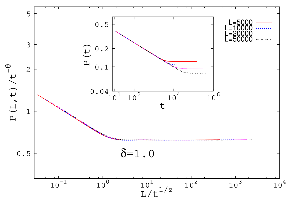
Figure 5: (Color online) The collapse of the scaled persistence probability against scaled time using $\theta=0.20\pm 0.002$ and $z=1.0\pm 0.002$ for different system sizes. Initial fraction of up spin $x=1/2$. Inset shows the unscaled data.

These exponents are universal in the sense that if one starts at any point on the phase boundary (i.e., with the initial fraction of up spins equal to $x_{c}(\delta)$), one gets the same values.

In the WI model, $z\simeq 1$ as in the BS model but the persistence exponent is different (by more than ten percent numerically). In fact, $\theta\sim 0.20$ obtained here is less than the BS model value ($\sim 0.235$), which is a bit counter-intuitive as the WI model is completely stochastic while the BS model is not. In the BS model, there is a ballistic motion of the surviving domain walls, which in the course of their motion will flip all the spins that appear on one of their boundaries. With high probability, these spins will flip once only so that if any flipping occurs it is more likely to affect the persistence probability. In the WI model, there will be motion of the domain walls in both directions (though less in comparison to the Ising model where pure random walk is executed before the domain walls are annihilated), such that the same spin may flip more than once with higher probability and obviously persistence will not be affected when a spin flips more than once. To check this, we have computed the distribution $g(n)$ of the number ($n$) of times a spin flips in both the models.

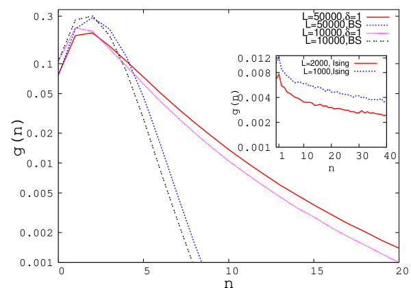
Figure 6: (Color online) The probability $g(n)$ that a spin flips $n$ number of times up to the time of reaching the equilibrium state is plotted against $n$ for both the BS model and the WI model (with $\delta=1$). Inset shows the same for the nearest neighbour Ising model.

The results, shown in Fig. 6, exhibit indeed that in the BS model, $g(1)$ is much higher compared to the WI model while probability that a spin flips a large number of times ($n>4$) is much less. (Roughly, for $n>3$, $\log g(n)\propto{-n}$ for the BS model and $\propto-\sqrt{n}$ for the WI model with $\delta=1$.) We have already seen that the probability of flipping $P_{f}(t)$ shows the same scaling behaviour in the two models and this shows why the persistence decays in a slower manner in the present model.

In comparison, in the Ising model, the persistence probability decays fastest although the domain walls perform pure random walk. Here, $P_{f}(t)\propto t^{-1/2}$ implies that domains survive much longer and as a result a larger number of spins are flipping at every step. So although $g(n)$ has a much slower decay the persistence probability decays much faster showing that the effect of the slower decay in the number of domain walls is more important than the unbiased random walk motion of each.

Stochasticity in the BS model has been introduced in several ways earlier by incorporating a parameter in the model sbpspr ; ps1 . In fact in ps1 , the domain sizes had been considered in the dynamics in a different manner. However, even such stochasticity in the BS model could not lead to any new dynamical behaviour ($z$ and $\theta$ were found to be equal to $\sim 1$ and $\sim 0.235$ respectively). On the other hand, the stochastic model considered here shows a different result for $\theta$ even for the unweighted model ($\delta=1$).

VI Concluding remarks

We have presented a stochastic binary opinion dynamics model with one parameter where the exit probability has a step function like behaviour even in one dimension, in contrast to other familiar models. One obtains a separatrix which is similar to that appearing in magnetic systems at zero field, separating regions of positive and negative magnetisation although in the latter one considers strictly the equilibrium behaviour. The results show finite size scaling where the scaling argument is $|x-x_{c}|L^{1/\nu}$ indicating that the width of the region where $f_{up}$ is not equal to unity or zero decreases as $L^{-1/\nu}$.

The unique behaviour of the exit probability may be present due to the effective long range interactions in the WI model. However it has been shown previously for the generalised voter and Sznajd models that the exit probability does not change its nature even if one makes the range of interaction infinite cast_sat ; przy . This indicates that the dynamical rule of WI model which handles the range of interaction in a subtly different manner could be responsible for the behaviour of the exit probability. A thorough study of similar models with domain size dependent dynamics is in progress to check this soham . One may also attempt to check the dependence of $\nu$ when the problem is considered in higher dimensions. It is also observed that there is a deviation from the mean field result unlike other models in one dimension. This deviation is attributed to the fact that the fluctuations which have been ignored (e.g., by taking $P_{1},P_{-1}$ independent of location and replacing all domain sizes by an average value) are indeed relevant. However, the deviation from mean field estimates is still small such that the mean field result can be considered as a first order calculation.

The other important and interesting result is that the persistence exponent of WI model is not only different but lowest among the well known models, including those where domain size dependent dynamics have been used. Thus the WI model is claimed to belong to a unique dynamical class in opinion dynamics models.

VII Acknowledgement

We are grateful to Deepak Dhar for a critical reading of an earlier version of the manuscript and for some useful discussions. SS acknowledges support from the UGC Dr. D. S. Kothari Postdoctoral Fellowship under grant No. F.4-2/2006(BSR)/13-416/2011(BSR). SB thanks the Department of Theoretical Physics, TIFR, for the use of its computational resources. PS thanks UPE (UGC) project for computational support.

References

- (1) P. C. Hohenberg and B. I. Halperin, Rev. Mod. Phys. 49, 435 (1977).
- (2) A. J. Bray, Adv. Phys. 43, 357 (1994).
- (3) D. Stauffer, in Encyclopedia of Complexity and systems Science edited by R. A. Meyers (Springer, New York, 2009).
- (4) C.Castellano, M.A.Munoz, R.Pastor-Satorras, Phys. Rev. E 80, 041129 (2009).
- (5) C. Castellano and R. P. Satorras Phys. Rev. E 83, 016113 (2011).
- (6) K. Sznajd-Weron and J. Sznajd, Int. J. Mod. Phys. C 11, 1157 (2000).
- (7) F. Slanina, K. Sznajd-Weron and P. Przybyla, Europhys. Lett., 82 18006 (2008).
- (8) C. Castellano, S. Fortunato and V. Loreto, Rev. Mod. Phys 81, 591 (2009).
- (9) R. Lambiotte and S. Redner, Europhys. Lett. 82, 18007 (2008).
- (10) S. Galam and A. C. R. Martins, Europhys. Lett. 48005 95 (2011) and the references therein.
- (11) P. Przybyla, K. Sznajd-Weron, and M. Tabiszewski, Phys. Rev. E 84, 031117 (2011)
- (12) D. Stauffer, A. O. Sousa and S. M. de Oliveira, Int. J. Mod. Phys. C, 11, 1239 (2000).
- (13) N. Crokidakis and P. M. C. de Oliveira, J. Stat. Mech. (2011) P11004 and the references therein.
- (14) B. Derrida, A. J. Bray and C. Godreche, J. Phys. A 27, L357 (1994).
- (15) Available election data do not provide the dynamical evolution of a voters’ decision but mainly the distribution of of votes obtained by the candidates (see e.g. A. Chatterjee, M. Mitrovic and S. Fortunato, Scientific Reports 3, 1049 (2013)). Thus comparing real data directly with our model at present is not possible. However, the fact that a change in government/winner happens quite often in elections implies that the loser in one election can emerge as a winner in the next, and the dynamics must be responsible for this effect.
- (16) S. Moscovici, Silent majorities and loud minorities, Communication Yearbook, 14, J.A. Anderson (Sage Publications Inc., 1990);
- (17) S. Galam, Eur. Phys. J. B, 25, 403 (2002).
- (18) The model was very briefly discussed in ps1 , only the dynamic results were mentioned which are not fully correct.
- (19) S. Biswas and P. Sen, Phys. Rev. E 80, 027101 (2009).
- (20) G. Manoj and P. Ray, Phys. Rev. E 62, 7755 (2000); J. Phys. A 33, 5489 (2000).
- (21) S. Biswas, A. K. Chandra, and P. Sen, Phys. Rev. E 78,041119 (2008).
- (22) P. Sen, Phys. Rev. E 81, 032103 (2010).
- (23) S. Biswas, P. Sen and P. Ray, Journal of Physics : Conf. Series 297, 012003 (2011).
- (24) P. Roy, S. Biswas and P. Sen (to be published).