Involutive Bases Algorithm Incorporating F₅ Criterion

Abstract

Faugère’s F₅ algorithm [13] is the fastest known algorithm to compute Gröbner bases. It has a signature-based and an incremental structure that allow to apply the F₅ criterion for deletion of unnecessary reductions. In this paper, we present an involutive completion algorithm which outputs a minimal involutive basis. Our completion algorithm has a nonincremental structure and in addition to the involutive form of Buchberger’s criteria it applies the F₅ criterion whenever this criterion is applicable in the course of completion to involution. In doing so, we use the G²V form of the F₅ criterion developed by Gao, Guan and Volny IV [14]. To compare the proposed algorithm, via a set of benchmarks, with the Gerdt-Blinkov involutive algorithm [19] (which does not apply the F₅ criterion) we use implementations of both algorithms done on the same platform in Maple.

url]http://compalg.jinr.ru/CAGroup/Gerdt/

url]www.amirhashemi.iut.ac.ir

1 Introduction

The most universal algorithmic tool in commutative algebra and algebraic geometry is Gröbner basis. The notion of Gröbner basis was introduced and an algorithm for its construction was designed in 1965 by Buchberger in his PhD thesis [6]. Later on [7], he discovered two criteria for detecting some unnecessary, and thus useless, reductions that made the Gröbner bases method practical for solving a wide class of problems in commutative algebra, algebraic geometry and in many other research areas of science and engineering (see, for example, [8]). However, that original Buchberger’s algorithm turned out to be too time and space consuming for many polynomial systems of scientific and industrial interest. In 1983, Lazard [26] proposed a new approach based on the linear algebra techniques to compute Gröbner bases. In 1988, Gebauer and Möller [16] reformulated Buchberger’s criteria in an efficient way. In 1999, Faugère [12] designed the F₄ algorithm to compute Gröbner bases. This algorithm stems from Lazard’s approach [26] and exploits fast linear algebra for manipulation with underlying sparse matrices. It has been efficiently implemented in Maple and Magma. In 2002, Faugère designed F₅ algorithm, an incremental algorithm, based on the F₅ criterion [13]. Ars and Hashemi [3] proposed a non-incremental version of F₅ by defining a new ordering on the signatures that made F₅ independent on the order of input polynomials. A correlation between Buchberger’s and Faugère’s approaches and methods was carefully analysed by Mora [28]. Recently Eder and Perry [10] simplified some of the steps in F₅ by constructing the reduced Gröbner basis at each step of the algorithm. Their algorithm called F₅C has been implemented in Singular and somewhat optimizes F₅. Then Gao, Guan and Volny IV in [14] presented G²V; a variant of the F₅ algorithm whose structure is simpler than that of F₅ and F₅C and moreover, according to the benchmarking done by the authors of G²V, the last algorithm may be more efficient than the other two signature-based algorithms. We refer to [33, 34, 11] and references therein for further information on signature-based algorithms.

Another theory which largely parallels the theory of Gröbner bases is the theory of involutive bases. This theory has its origin in the works of the French mathematician Janet. In the $20$s of the last century, he developed [25] a constructive approach to analysis of linear and certain quasi-linear systems of partial differential equations based on their completion to involution (see the recent book [32] and references therein). The Janet approach has been generalized to arbitrary polynomially non-linear differential systems by the American mathematician Thomas [35]. Based on the involutive methods as they have been presented in Pommaret’s book [31], Zharkov and Blinkov introduced in [36] the notion of involutive polynomial bases. The particular form of an involutive basis that they studied is nowadays called Pommaret basis [32].

Gerdt and Blinkov [19] proposed a more general concept of involutive bases for polynomial ideals and designed algorithmic methods to construct these bases. The basic underlying idea of the involutive approach to commutative algebra is to translate the methods originating from Janet’s approach into polynomial ideal theory in order to provide an algorithmic method for construction of polynomial involutive bases by combining algorithmic ideas in the theory of Gröbner bases and constructive ideas in the theory of involutive differential systems. In doing so, Gerdt and Blinkov [19] introduced the concept of involutive monomial division and established two criteria to avoid some useless involutive reductions. This led to a computational tool (see the web pages http://invo.jinr.ru and http://wwwb.math.rwth-aachen.de/Janet/ ) which can be considered as an efficient alternative (http://cag.jinr.ru/wiki/Benchmarking_for_polynomial_ideals) to the conventional Buchberger’s algorithm (note that any involutive basis is also a Gröbner basis). Apel and Hemmecke [2] discovered that there are two more criteria for detecting unnecessary involutive reductions (see also [Gerdt (2002)]) which, in the aggregate with the criteria by Gerdt and Blinkov [19], are equivalent to Buchberger’s criteria. The first author decribed in [18] a computationally efficient algorithm for involutive and Gröbner bases using all these criteria. Different versions of involutive algorithms [18, 19, 36] based on the concept of involutive division by Gerdt and Blinkov have been implemented in Reduce, Singular, Macaulay2, Maple and very recently in CoCoA. The fastest implementation is the one done in GINV [21]. For application of involutive bases to commutative algebra and to algebraic-geometric theory of partial differential equations we refer to Seiler’s book [32].

The conventional and involutive full normal forms modulo an involutive basis are equal [19]. Thereby, a natural question that arises is: How to incorporate the F₅ criterion into an involutive algorithm? In the given paper, we answer this question by proposing a new structure for the algorithm described in [18]. We shall refer to the last as the Gerdt-Blinkov involutive (GBI) algorithm. Our structure allows to exploit the F₅ criterion. For the sake of simplicity, we use here the G²V version of the criterion. Our new algorithm is not incremental since at each step we must consider the set of multiplicative and nonmultiplicative variables for the whole set of polynomials in the intermediate basis including the input ones (see Section 4). However, by using the signature characterization inherent in any version of the F₅ algorithm, we provide an F₅-consistent involutive completion of the input polynomial set. Such a completion applies the F₅ criterion as much as possible and ends up with an involutive basis. Then a minimal involutive basis is constructed from the last basis. We have implemented the new algorithm in Maple for the Janet division [19] and for the $\succ_{\mathop{\mathrm{alex}}\nolimits}$-division [22]. In order to analyse the new algorithm experimentally, via some benchmarks, and to make its comparison with the GBI algorithm at the same implementation platform, we implemented the last algorithm in Maple for both involutive divisions as well.

The paper is organized as follows. Section 2 contains some basic definitions and notations related to the theory of involutive bases, and the algorithm for construction of minimal such bases in its simplest form [18]. In Section 3 we present briefly the F₅ criterion and its G²V modification. Section 4 is devoted to the description of our new involutive algorithm for computing minimal involutive bases. At the end of this section, we give an illustrating example for the proposed algorithm. In Section 5 we present our experimental comparison of the new algorithm with the GBI algorithm.

2 Involutive bases

In this section, we recall some basics from the theory of involutive bases and briefly describe the algorithm for their construction in its simplest form [18].

Let $K$ be a field and $R:=K[x_{1},\ldots,x_{n}]$ be the polynomial ring in the variables $x_{1},\ldots,x_{n}$ over $K$. Below, we denote a monomial $x_{1}^{\alpha_{1}}\cdots x_{n}^{\alpha_{n}}\in R$ by ${\bf x}^{\alpha}$ where $\alpha=(\alpha_{1},\ldots,\alpha_{n})\in\mathbb{N}^{n}$ is a sequence of non-negative integers. We shall use the notations ${\mbox{\rm deg}}_{i}({\bf x}^{\alpha}):=\alpha_{i}$ and ${\mbox{\rm deg}}({\bf x}^{\alpha}):=\sum_{i}\alpha_{i}$. An admissible monomial ordering on $R$ is a total order $\prec$ on the set of all monomials such that
      (i) $1\prec\mathbf{x}^{\alpha}\ \text{for all}\ \mathbf{x}^{\alpha}\neq 1$ ,  (ii) $\mathbf{x}^{\alpha}\prec\mathbf{x}^{\beta}\ \text{implies}\ \mathbf{x}^{\alpha+\gamma}\prec\mathbf{x}^{\beta+\gamma}\ \text{for all}\ \alpha,\beta,\gamma\in\mathbb{N}^{n}$ .

The typical examples of such monomial orderings denoted respectively by $\prec_{\mathop{\mathrm{lex}}\nolimits}$ and $\prec_{\mathop{\mathrm{degrevlex}}\nolimits}$ are lexicographical and degree-reverse-lexicographical. Given monomials ${\bf x}^{\alpha}$ and ${\bf x}^{\beta}$, ${\bf x}^{\alpha}\prec_{\mathop{\mathrm{lex}}\nolimits}{\bf x}^{\beta}$ if the left-most non-zero entry of $\beta-\alpha$ is positive; ${\bf x}^{\alpha}\prec_{\mathop{\mathrm{degrevlex}}\nolimits}{\bf x}^{\beta}$ if ${\mbox{\rm deg}}({\bf x^{\alpha}})>{\mbox{\rm deg}}({\bf x^{\beta}})$ or ${\mbox{\rm deg}}({\bf x^{\alpha}})={\mbox{\rm deg}}({\bf x^{\beta}})$ and the right most non-zero entry of $\beta-\alpha$ is negative.

Let ${{\mathcal{I}}}=\langle f_{1},\ldots,f_{k}\rangle$ be the ideal in $R$ generated by the polynomials $f_{1},\ldots,f_{k}\in R$. Furthermore, let $f\in R$ and $\prec$ be a monomial ordering on $R$. The leading monomial of $f$ is the greatest monomial (with respect to $\prec$) occurring in $f$, and we denote it by ${\mathrm{LM}}(f)$. Respectively, the leading term of $f$ is denoted by ${\mathrm{LT}}(f)$ and the leading coefficient by ${\mathrm{LC}}(f)$. If $F\subset R$ is a set of polynomials, we denote by ${\mathrm{LM}}(F)$ the set $\{{\mathrm{LM}}(f)\ \mid\ f\in F\}$. The leading monomial ideal of ${{\mathcal{I}}}$ is defined to be ${\mathrm{LM}}({{\mathcal{I}}})=\langle{\mathrm{LM}}(f)\ \mid\ f\in{{\mathcal{I}}}\rangle.$ A finite set $G\subset{{\mathcal{I}}}$ is called a Gröbner basis of ${{\mathcal{I}}}$ if ${\mathrm{LM}}({{\mathcal{I}}})=\langle{\mathrm{LM}}(G)\rangle$. We refer to the book by Becker and Weispfenning [4] for more details on Gröbner bases.

We recall below the definition of involutive bases. For this purpose, we describe first the notion of an involutive division [19] which is a restricted monomial division [18] that, together with a monomial ordering, determines properties of an involutive basis. This makes the main difference between involutive bases and Gröbner bases. The idea is to partition the variables into two subsets of multiplicative and nonmultiplicative variables, and only the multiplicative variables can be used in the divisibility relation.

Definition 1.

([19]) An involutive division ${{\mathcal{L}}}$ on the set of monomials of $R$ is given, if for any finite set $U$ of monomials and any $u\in U$, the set of variables is partitioned into the subsets of multiplicative $M_{{\mathcal{L}}}(u,U)$ and nonmultiplicative $NM_{{\mathcal{L}}}(u,U)$ variables such that the following three conditions hold:

• $u,v\in U,\ u\cdot{{{\mathcal{L}}}(u,U)}\cap v\cdot{{{\mathcal{L}}}(v,U)}\neq\emptyset$ implies $u\in v\cdot{{{\mathcal{L}}}(v,U)}$ or $v\in u\cdot{{{\mathcal{L}}}(u,U)}$,

• $u,v\in U,\ v\in u\cdot{{{\mathcal{L}}}(u,U)}$ implies ${{{\mathcal{L}}}(v,U)}\subset{{{\mathcal{L}}}(u,U)}$,

• $u\in V$ and $V\subset U$ implies ${{{\mathcal{L}}}(u,U)}\subset{{{\mathcal{L}}}(u,V)}$,

where ${{\mathcal{L}}}(u,U)$ denotes the monoid generated by the variables in $M_{{\mathcal{L}}}(u,U)$. If $v\in u\cdot{{\mathcal{L}}}(u,U)$ then $u$ is called ${{\mathcal{L}}}$-(involutive) divisor of $v$ and the involutive divisibility relation is denoted by $u\mid_{{\mathcal{L}}}v$. If $v$ has no involutive divisors in a set $U$, then it is called ${{\mathcal{L}}}$-irreducible modulo $U$.

There are involutive divisions based on the classical partitions of variables suggested by Janet [25] and Thomas [35]. In this paper, we are also concerned with the wide class [22] of involutive divisions determined by a total monomial ordering $\sqsupset$ such that it is either admissible or the inverse of an admissible ordering, and by a permutation $\sigma$ on the indices of variables:

$$(\ \forall u\in U\ )\ \ [\ NM_{\sqsupset}(u,U)=\bigcup_{v\in U\setminus\{u\}}NM_{\sqsupset}(u,\{u,v\})\ ]$$ (1)

$$NM_{\sqsupset}(u,\{u,v\}):=\left\{\begin{array}[]{l}\text{ if }u\sqsupset v\text{ or }(u\sqsubset v\wedge v\mid u)\text{ then }\emptyset\\[2.84544pt] \text{ else }\{x_{\sigma(i)}\},\ i=\min\{j\mid{\mbox{\rm deg}}_{\sigma(j)}(u)<{\mbox{\rm deg}}_{\sigma(j)}(v)\}\,.\\ \end{array}\right.$$ (2)

Throughout the given paper, ${{\mathcal{L}}}$ is assumed to be either the division in this class, denoted by $\sqsupset$-division, or the Thomas division. If we consider the monomial ordering $\sqsupset$ to be the lexicographical ordering, then (1)-(2) generates the Janet division. As to the Thomas division (denoted by ${\mathcal{T}}$), it satisfies (1), but unlike (2) this division is not linked to a total monomial ordering. Instead,

$$NM_{{\mathcal{T}}}(u,\{u,v\}):=\{\,x\mid{\mbox{\rm deg}}_{x}(u)<{\mbox{\rm deg}}_{x}(v)\,\}\,.$$ (3)

Now, we define an involutive basis.

Definition 2.

([18]) Let ${{\mathcal{I}}}\subset R$ be an ideal, $\prec$ a monomial ordering on $R$ and ${{\mathcal{L}}}$ an involutive division. A finite set $G\subset{{\mathcal{I}}}$ is an involutive basis (or ${{\mathcal{L}}}$-basis) of ${{\mathcal{I}}}$ if for any $f\in{{\mathcal{I}}}$ there is $g\in G$ such that ${\mathrm{LM}}(g)\mid_{{\mathcal{L}}}{\mathrm{LM}}(f)$. If $U\subset R$ is a finite monomial set, then a monomial set $\bar{U}$ is called ${{\mathcal{L}}}$-completion of $U\subseteq\bar{U}$ if $\bar{U}$ is an ${{\mathcal{L}}}$-basis of $\langle U\rangle$.

From this definition and from that of a Gröbner basis [4, 6] it follows that an involutive basis is a Gröbner basis of the ideal that it generates, but the converse is not always true. Noetherianity of a division ${{\mathcal{L}}}$ [19, 22] guarantees the existence of an ${{\mathcal{L}}}$-basis.

Proposition 3.

([19]) Any ideal has a finite ${{\mathcal{L}}}$-basis.

Remark 4.

By using an involutive division in polynomial rings, we obtain an involutive division algorithm [19]. Given a finite polynomial set $F$ and a monomial ordering, we denote by ${\rm{NF}}_{{\mathcal{L}}}(f,F)$ the remainder in ${{\mathcal{L}}}$-division of $f$ by $F$.

For an involutive division ${{\mathcal{L}}}$, the following theorem provides an algorithmic characterization of involutive basis for a given ideal that is an involutive analogue of the Buchberger characterization of a Gröbner basis.

Theorem 5.

([19]) Let ${{\mathcal{I}}}\subset R$ be an ideal, $\prec$ a monomial ordering on $R$ and ${{\mathcal{L}}}$ an involutive division. Then a finite generating set $G\subset{{\mathcal{I}}}$ is an ${{\mathcal{L}}}$-basis of ${{\mathcal{I}}}$ if for each $f\in G$ and each $x\in NM_{{\mathcal{L}}}({\mathrm{LM}}(f),{\mathrm{LM}}(G))$, we have ${\rm{NF}}_{{\mathcal{L}}}(x\cdot f,G)=0$.

Definition 6.

([19]) An involutive basis $G$ is called minimal if for any other involutive basis $\tilde{G}$ of $\langle G\rangle$ the inclusion ${\mathrm{LM}}(G)\subseteq{\mathrm{LM}}(\tilde{G})$ holds. Similarly, a minimal involutive completion of a monomial set is a subset of any other involutive completion of this set.

A minimal involutive basis being monic and ${{\mathcal{L}}}$-autoreduced, i.e. satisfying

$$(\forall g\in G)\ [\,g={\rm{NF}}_{{\mathcal{L}}}(g,G\setminus\{g\})\,]$$

is unique for a given ideal and a monomial ordering. Similarly, the minimal monomial involutive completion is uniquely defined.

Proposition 7.

For any $\sqsupset$-division and any finite set $U$ of monomials the following inclusion holds

$$(\,\forall u\in U\,)\ [\,NM_{\sqsupset}(u,U)\subseteq NM_{{\mathcal{T}}}(u,U)\,]\,,\quad\bar{U}_{\sqsupset}\subseteq\bar{U}_{{\mathcal{T}}}$$ (4)

where $\bar{U}_{\sqsupset}$ and $\bar{U}_{{\mathcal{T}}}$ denotes the minimal completion of $U$ for the $\sqsupset$-division and for the Thomas division, respectively.

Proof. The first inclusion (for nonmultiplicative variables) is an obvious consequence of (2) and (3). The second inclusion is an immediate consequence of the first one.    $\Box$

Remark 8.

The minimal Thomas completion $\bar{U}_{{\mathcal{T}}}$ of a monomial set $U$ is given [19] by

$$\bar{U}_{{\mathcal{T}}}=\{\,u\in\langle U\rangle\mid deg_{i}(u)\leq\max\{\,{\mbox{\rm deg}}_{i}(v)\mid v\in U\,\}\,,\ i=1,\ldots,n\,\}\,.$$ (5)

Based on Theorem 5, one can design an algorithm to compute involutive bases. We recall here the InvBas (InvolutiveBasis) algorithm from [18]. The algorithm outputs a minimal involutive basis.

As it is emphasized in [18], in comparison to the algorithm of the second paper in [19], another selection strategy is used in InvBas that optimizes the displacement done in the for-loop (lines 8-11). By this strategy, a polynomial is chosen in line 5 whose leading monomial has no proper divisors among the leading monomials in $Q$. However, the below version of the GBI algorithm is still not efficient in practice, since it repeatedly processes the same prolongations and does not apply any criterion to avoid superfluous reductions.

Algorithm InvBas

0:  $F$, a set of polynomials; ${{\mathcal{L}}}$, an involutive division; $\prec$, a monomial ordering 0:  a minimal involutive basis of $\langle F\rangle$ 1:  Select $f\in F$ with no proper divisor of ${\mathrm{LM}}(f)$ in ${\mathrm{LM}}(F)$; 2:  $G:=\{f\}$; 3:  $Q:=F\setminus G$; 4:  while $Q\neq\emptyset$ do 5:     Select and remove $p\in Q$ with no proper divisor of ${\mathrm{LM}}(p)$ in ${\mathrm{LM}}(Q)$; 6:     $h:={\rm{NF}}_{{\mathcal{L}}}(p,G)$; 7:     if $h\neq 0$ then 8:        for $g\in G$ such that ${\mathrm{LM}}(g)$ is properly divisible by ${\mathrm{LM}}(h)$ do 9:           $Q:=Q\cup\{g\}$; 10:           $G:=G\setminus\{g\}$; 11:        end for 12:        $G:=G\cup\{h\}$; 13:        $Q:=Q\cup\{x\cdot g\ |\ g\in G,x\in NM_{{\mathcal{L}}}({\mathrm{LM}}(g),{\mathrm{LM}}(G))\}$; 14:     end if 15:  end while 16:  return ($G$)

The improved version of the algorithm which is also presented in [18] clears away the repeated processing of prolongations and applies the involutive form of Buchberger’s criteria. Below, we suggest one more algorithmic improvement which, in addition to the indicated ones, admits application of the F₅ criterion for deletion of useless reductions.

3 F₅ criterion and G²V algorithm

This section presents the theory behind the F₅ algorithm. After recalling some notations and definitions, we state the main theorem of [13] which is the cornerstone of the F₅ algorithm. To this end, we consider the recent paper [11] due to Eder and Perry. Finally, we present briefly the G²V algorithm [14] further developed in [15].

Let ${{\mathcal{I}}}=\langle f_{1},\ldots,f_{k}\rangle\subset R=K[x_{1},\ldots,x_{n}]$ be the ideal in $R$ generated by the polynomials $f_{1},\ldots,f_{k}$, $R^{k}$ be a free $R$-module of rank $k$ and ${\mathbf{e}_{1}},\ldots,{\mathbf{e}_{k}}$ be its canonical basis. For the sake of simplicity assume that each $f_{i}$ is monic, i.e. ${\mathrm{LC}}(f_{i})=1$. A module monomial is an element in $R^{k}$ of the form $m{\mathbf{e}_{i}}$ where $m\in R$ is a monomial. Let us denote the set of all module monomials by $\mathbf{M}$. A monomial ordering $\prec$ on $R$ can be extended to a module monomial ordering on $\mathbf{M}$, denoted by $<$, as follows

$$\sum^{j}_{i=1}{g_{i}\cdot{\mathbf{e}_{i}}}<\sum^{\ell}_{i=1}{h_{i}\cdot{\mathbf{e}_{i}}}\ \ {\rm if}\ \ \left\{\begin{array}[]{lcl}j>\ell&{\rm and}&h_{\ell}\neq 0\ {\rm or}\\[-5.69046pt] j=\ell&{\rm and}&{\mathrm{LM}}(g_{j})\prec{\mathrm{LM}}(h_{j}),\ g_{j}\cdot h_{j}\neq 0.\end{array}\right.$$

Definition 9.

Let $f\in{\mathcal{I}}$ and $1\leq j\leq k$ be the smallest integer for which $h_{j}\neq 0$ in $f=\sum_{i=1}^{k}h_{i}f_{i}$. Then, the module monomial ${\mathrm{LM}}(h_{j})\,{\mathbf{e}_{j}}$ is called a natural signature of $f$. Under the assumption, ${\mathrm{LM}}(h_{j}){\mathbf{e}_{j}}$ is the greatest module monomial w.r.t. $<$ occurring in $\sum_{i=1}^{k}h_{i}{\mathbf{e}_{i}}\in R^{k}$. Denote by ${\rm{sig}}(f)$ the set of all natural signatures of $f$. As one can easily see, $<$ is a well-ordering on $\mathbf{M}$ and thus ${\rm{sig}}(f)$ has a unique minimal element, which is called the minimal natural signature of $f$.

Let $f\in R$ and $m{\mathbf{e}_{i}}={\rm{sig}}(f)$. Then the pair $(m{\mathbf{e}_{i}},f)\in R^{k}\times R$ is called a labelled polynomial associated to $f$. We shall denote the set of all labelled polynomials by ${\bf L}$, and from this point on we shall write ${\mathcal{S}}(f)$ for the minimal signature associated to $f$ by the signature based algorithm under consideration.

Definition 10.

Let $r=(m{\mathbf{e}_{i}},f)\in{\bf L}$. Then $f$, $m{\mathbf{e}_{i}}$ and $i$ are, respectively, called the polynomial part, signature and index of $r$ and we denote them by ${\rm{poly}}(r)$, ${\mathcal{S}}(r)$ and index$(r)$. We define also ${\mathrm{LM}}(r),{\mathrm{LC}}(r)$ and ${\mathrm{LT}}(r)$ as ${\mathrm{LM}}(f),{\mathrm{LC}}(f)$ and ${\mathrm{LT}}(f)$, respectively. Furthermore, the labelled polynomial $r$ can be multiplied by a monomial $u$ and by an element $c\in K$ of the ground field in accordance to the rules $ur=(um{\mathbf{e}_{i}},uf)$ and $cr=(m{\mathbf{e}_{i}},cf)$.

Denote by $\psi$ the following map:

$$\begin{array}[]{cccl}\psi:&R^{k}&\rightarrow&R\\[-5.69046pt] &(g_{1},\ldots,g_{k})&\mapsto&g_{1}f_{1}+\cdots+g_{k}f_{k}.\end{array}$$

A labelled polynomial $r=({\mathcal{S}}(r),{\rm poly}(r))$ is called admissible if there exists ${\bf g}\in R^{k}$ such that $\psi({\bf g})={\rm poly}(r)$ and the greatest module monomial w.r.t. $<$, occurring in ${\bf g}$ is ${\mathcal{S}}(r)$. It is easy to check that with the above notations, $um{\mathbf{e}_{i}}\in{\rm{sig}}(uf)$, and hence the multiplication rules in Definition 10 preserve the admissibility. Let us explain now the reduction algorithm used in ${\bf L}$. In this case, the reduction is more restrictive than the usual polynomial reduction. If $(m{\mathbf{e}_{i}},f)$ is reducible by $(m^{\prime}{\mathbf{e}_{j}},g)$; i.e. $t{\mathrm{LM}}(g)={\mathrm{LM}}(f)$ for a monomial $t\in R$, then one of the following cases holds.

• (safe reduction): If $tm^{\prime}{\mathbf{e}_{j}}<m{\mathbf{e}_{i}}$, then the reduction is performed as $(m{\mathbf{e}_{i}},f-tg)$.

• (unsafe reduction): If $tm^{\prime}{\mathbf{e}_{j}}\geq m{\mathbf{e}_{i}}$, then the signature is changed at the reduction step, and such a reduction is not performed.

This reduction algorithm provides an alternative definition (cf.  [4], Definition 5.59) of standard representation for labelled polynomials.

Definition 11.

Let $P\subset{\bf L}$ be a finite set, and $r,t\in{\bf L}$ with $f:={\rm{poly}}(r)\neq 0$. We say that $r$ has a $t$-representation w.r.t. $P$ if $f=\sum_{p_{i}\in P}{h_{i}{\rm{poly}}(p_{i})}$ $(h_{i}\in{cR})$ and for all $p_{i}\in P$ with ${\rm{poly}}(p_{i})\neq 0$ the following relations hold:

$${\mathrm{LM}}(h_{i}){\mathrm{LM}}(p_{i})\preceq{\mathrm{LM}}(t)\ \ {\rm and}\ \ {\mathrm{LM}}(h_{i}){\mathcal{S}}(p_{i})\leq{\mathcal{S}}(r).$$

This property is written as $r=\mathcal{O}_{P}(t)$. We shall also write $r=o_{P}(t)$ if there exists a labelled polynomial $t^{\prime}\in A$ satisfying ${\mathcal{S}}(t^{\prime})\leq{\mathcal{S}}(t)$ and ${\mathrm{LM}}(t^{\prime})\prec{\mathrm{LM}}(t)$ such that $r=\mathcal{O}_{P}(t^{\prime})$. A $t$-representation of $r$ is called standard if ${\mathrm{LM}}(t)={\mathrm{LM}}(r)$.

To state a Buchberger-like criterion for labelled polynomials (Theorem 12), we need to define the $S$-polynomial of two labelled polynomials. Suppose that $f,g\in R$ are two polynomials. The conventional $S$-polynomial of $f$ and $g$ is defined to be

$${\mathrm{Spoly}}(f,g)=\frac{{\rm lcm}({\mathrm{LM}}(f),{\mathrm{LM}}(g))}{{\mathrm{LT}}(f)}f-\frac{{\rm lcm}({\mathrm{LM}}(f),{\mathrm{LM}}(g))}{{\mathrm{LT}}(g)}g\,.$$

Let now $r=({\mathcal{S}}(r),f)$ and $s=({\mathcal{S}}(s),g)$ be two admissible labelled polynomials with $u={\rm lcm}({\mathrm{LM}}(f),{\mathrm{LM}}(g))/{\mathrm{LM}}(f),v={\rm lcm}({\mathrm{LM}}(f),{\mathrm{LM}}(g))/{\mathrm{LM}}(g)$. If $v{\mathcal{S}}(s)<u{\mathcal{S}}(r)$, we define the labelled $S$-polynomial of $r$ and $s$ to be ${\mathrm{Spoly}}(r,s)=(u{\mathcal{S}}(r),{\mathrm{Spoly}}(f,g))$. Otherwise, we do not consider such an $S$-polynomial, see [11] for more details.

Theorem 12.

([11]) Let ${{\mathcal{I}}}=\langle f_{1},\ldots,f_{k}\rangle\subset R$ and let $G\subset{\bf L}$ be a finite set of admissible labelled polynomials such that

• for all $1\leq i\leq k$ there exists $r_{i}\in G$ such that $f_{i}={\rm{poly}}(r_{i})$,

• for each pair $(r_{i},r_{j})\in G\times G$ either $u_{i}{\mathcal{S}}(r_{i})=u_{j}{\mathcal{S}}(r_{j})$, ${\mathrm{Spoly}}(r_{i},r_{j})=0$ or ${\mathrm{Spoly}}(r_{i},r_{j})=o_{G}(u_{s}\cdot r_{s})$ where $u_{s}={\rm lcm}({\mathrm{LM}}(r_{i}),{\mathrm{LM}}(r_{j}))/{\mathrm{LM}}(r_{s})$ for $s\in\{i,j\}$.

Then the set $\{{\rm{poly}}(r)\ |\ r\in G\}$ is a Gröbner basis of ${{\mathcal{I}}}$.

All algorithms to compute a Gröbner basis which take “signatures” into account are called signature-based algorithms, see [11]. Most of these algorithms, like Faugère’s F₅ algorithm [13] are described incrementally to apply the F₅ criterion. The F₅ algorithm computes sequentially the Gröbner bases of the ideals

$$\langle f_{k}\rangle,\langle f_{k-1},f_{k}\rangle,\ldots,\langle f_{1},\ldots,f_{k}\rangle.$$

Definition 13.

Let ${{\mathcal{I}}}=\langle f_{1},\ldots,f_{k}\rangle\subset R$. An admissible labelled polynomial $(m{\mathbf{e}_{i}},f)$ is called normalized, if $m\notin{\mathrm{LM}}(\langle f_{i+1},\ldots,f_{k}\rangle)$. A pair $(r_{1},r_{2})$ of admissible labelled polynomials is normalized if $u_{i}r_{i}$ and $u_{j}r_{j}$ are normalized where $u_{s}={\rm lcm}({\mathrm{LM}}(r_{i}),{\mathrm{LM}}(r_{j}))/{\mathrm{LM}}(r_{s})$ for $s\in\{i,j\}$.

Theorem 14.

(F₅ criterion) By the assumptions of Theorem 12, the $S$-polynomial of a non-normalized pair $(r_{i},r_{j})\in G\times G$ has a standard representation w.r.t. $G$, and therefore, it is superfluous.

Proof. See [13], Theorem 1.    $\Box$

The F₅ algorithm, in its original form [13], as the first signature-based algorithm is rather difficult to understand and to implement. Gao, Guan and Volny IV [14] (see also [15]) presented an algorithm called G²V which may be considered as a version of the F₅ algorithm. This version seems to be simpler and more efficient than the original F₅ (cf. the benchmarking in [14]). By this reason, we use G²V to apply the F₅ criterion in construction of involutive bases.

To explain the structure of G²V, assume that $G=\{g_{1},\ldots,g_{s}\}$ is a Gröbner basis of $\langle f_{i+1},\dots,f_{k}\rangle$ where $1\leq i\leq k-1$. Our goal is to compute a Gröbner basis of $\langle f_{i},\dots,f_{k}\rangle$. Much like F₅C [10], G²V uses the reduced Gröbner basis obtained at the preceding step of the algorithm. The structure of polynomials in G²V is slightly different from that mentioned before. As a labelled polynomial, G²V considers a pair $(m,f)\in R^{2}$ where $m$ is a monomial and $f\in R$ is a polynomial. The monomial $m$ is called the signature of the pair. A pair $(m,f)$ is admissible, if there exists $p\in R$ with $pf_{i}\equiv f$ mod $G$ such that ${\mathrm{LM}}(p)=m$. This is consistent with the representation of this labelled polynomial $(m{\mathbf{e}_{i}},f)$ in F₅.

Hereafter, we shall consider only admissible labelled polynomials and omit the term ‘admissible’. Initially, G²V considers the labelled polynomials $(0,g_{1}),\ldots,(0,g_{s})$ and $(1,g)$ where $g$ is the normal form of $f_{i}$ modulo $G$. Then, it creates the J(oint)-pairs of $(1,g)$ and of the other labelled polynomials. By definition, the J-pair of two labelled polynomials $(m,f)$ and $(m^{\prime},f^{\prime})$ is the labelled polynomial of the form $(tm,tf)$ with $t={\rm lcm}({\mathrm{LM}}(f),{\mathrm{LM}}(f^{\prime}))/{\mathrm{LM}}(f)$ and $t^{\prime}={\rm lcm}({\mathrm{LM}}(f),{\mathrm{LM}}(f^{\prime}))/{\mathrm{LM}}(f^{\prime})$ satisfying ${\mathrm{LM}}(t^{\prime}f^{\prime})\preceq{\mathrm{LM}}(tf)$.

G²V takes the J-pair with the smallest signature and repeatedly performs only regular top-reductions of this pair as long as such regular top-reduction is possible. A labelled polynomial $(m,f)$ is top-reducible by another labelled polynomial $(m^{\prime},f^{\prime})$ if there is a monomial $t\in R$ such that ${\mathrm{LM}}(f)=t{\mathrm{LM}}(f^{\prime})$ and $tm^{\prime}\prec m$. The corresponding top-reduction is defined as $(m,f)-t(m^{\prime},f^{\prime})=(m,f/{\mathrm{LC}}(f)-tf^{\prime}/{\mathrm{LC}}(f^{\prime}))$. If $tm^{\prime}=m$, then the reduction is called super, otherwise it is called regular.

Let $(m,f)$ be the result of reduction of a labelled polynomial. If $f\neq 0$, then $(m,f)$ is added to the current Gröbner basis, and the new J-pairs are formed. If $f=0$, then G²V uses $m$ to delete useless J-pairs. Namely, a labelled polynomial $(m^{\prime},f^{\prime})$ can be discarded [14] if $m^{\prime}\neq 0$ and $m\mid m^{\prime}$. In doing so, this kind of reduction is considered in [14] as a super top-reduction too (see also [15]). We shall also say that $(m^{\prime},f^{\prime})$ is super top-reducible by $(m,0)$ when $m\mid m^{\prime}$.

Now, we state and prove the theorem which stems from the results of paper [14] and provides the correctness of the G²V algorithm (cf. [15], Theorem 2.3) and thereby the correctness of applying the F₅ criterion in G²V.

Theorem 15 (G²V form of F₅ criterion).

Let $G$ be a Gröbner basis of $\langle f_{i+1},\dots,f_{k}\rangle$ and $G^{\prime}$ the output of G ²V. Then the set $T=\{f\ |\ (m,f)\in G^{\prime}\}$ is a Gröbner basis of $\langle f_{i},\dots,f_{k}\rangle$, if for each J-pair $(tm,tf)$ of the elements in $G^{\prime}$ one of the following conditions holds:

1. $(tm,tf)$ reduces to zero on the regular top-division by $G^{\prime}$.

2. $tm$ is multiple of an element in ${\mathrm{LM}}(G)$.

3. $(tm,tf)$ reduces to $(tm,g)$ on the regular top-division by $G^{\prime}$ so that $(tm,g)$ is no longer regular top-reducible by $G^{\prime}$, and $(tm,g)$ is super top-reducible by $G^{\prime}$.

4. $m^{\prime}\mid tm$ where $m^{\prime}$ is the signature of a labelled polynomial $(m^{\prime},0)$ obtained during the computation of $G^{\prime}$.

Proof. We must prove that for each J-pair $(tm,tf)$ of the elements in $G^{\prime}$, $tf$ has a standard representation w.r.t. $T$ (see [4], Theorem 5.64). The reducibility of the pair to zero yields immediately the standard representation for $(tm,tf)$. If the second condition holds, the pair is not normalized and we refer to [13], Theorem 1 (see also [28]). To prove the third item, suppose that $(tm,tf)$ reduces to $(tm,g)$ on the regular top-division by $G^{\prime}$, and $(tm,g)$ is super top-reducible by $(m^{\prime},f^{\prime})\in G^{\prime}$, i.e. $tm=sm^{\prime}$ and $t{\mathrm{LM}}(g)=s{\mathrm{LM}}(f^{\prime})$ for some monomial $s\in R$. Note that $(tm,g)$ may be super top-reducible by an element $(m^{\prime},0)$. In this case, which corresponds to the forth condition, we consider $f^{\prime}=0$. From admissibility of $(tm,g)$ and $(m^{\prime},f^{\prime})$ we can write $g=p_{i}f_{i}+\sum_{j=i+1}^{k}p_{j}f_{j}$ and $f^{\prime}=p^{\prime}_{i}f_{i}+\sum_{j=i+1}^{k}p^{\prime}_{j}f_{j}$ where $p_{j},p^{\prime}_{j}\in R$, $p_{i},p^{\prime}_{i}$ are monic, ${\mathrm{LM}}(p_{i})=tm$ and ${\mathrm{LM}}(p^{\prime}_{i})=m^{\prime}$. In that follows we denote $p-{\mathrm{LT}}(p)$ by ${\mathrm{tail}}(p)$ for a polynomial $p$. Thus,

$$g = tmf_{i}+{\mathrm{tail}}(p_{i})f_{i}+\sum_{j=i+1}^{k}p_{j}f_{j}$$

$$= sm^{\prime}f_{i}+{\mathrm{tail}}(p_{i})f_{i}+\sum_{j=i+1}^{k}p_{j}f_{j}$$

$$= sf^{\prime}-s\cdot{\mathrm{tail}}(p^{\prime}_{i})f_{i}-\sum_{j=i+1}^{k}sp^{\prime}_{j}f_{j}+{\mathrm{tail}}(p)f_{i}+\sum_{j=i+1}^{k}p_{j}f_{j}$$

$$= sf^{\prime}+({\mathrm{tail}}(p_{i})-s\cdot{\mathrm{tail}}(p^{\prime}_{i}))f_{i}+\sum_{j=i+1}^{k}(p_{j}-sp^{\prime}_{j})f_{j}\,.$$

This implies that polynomial $g-sf^{\prime}$ can be written as

$$({\mathrm{tail}}(p_{i})-s\cdot{\mathrm{tail}}(p^{\prime}_{i}))f_{i}+\sum_{j=i+1}^{k}(p_{j}-sp^{\prime}_{j})f_{j}\,.$$

In accordance to the choice of monomial ordering made in Section 2, the signature of labelled polynomial with this polynomial part is strictly less than $tm$. Therefore, $tf$ has a standard representation w.r.t. $T$.    $\Box$

Remark 16.

In the G²V algorithm, there are usually many J-pairs with the same signature. In this case Gao, Volny IV and Wang [15] claim that one can just store one J-pair $(m,f)$ whose polynomial part $f$ has the minimal leading monomial and discard all other J-pairs with signature $m$ (see [15], Theorem 2.3 for more details).

Remark 17.

Until recent papers by Huang [24], by Pan, Hu and Wang [29] and by Galkin[30] there has not been strong evidence for termination of the F₅ (and respectively G²V) algorithm. Based on the results of [24], in their preprint [15] Gao, Volny IV and Wang formulated the termination condition as compatibility of the monomial ordering $\succ$ with the module monomial ordering $>$:

$${\mathrm{LM}}(f)\mathbf{e}_{i}>{\mathrm{LM}}(g)\mathbf{e}_{i}\ \ \text{if and only if}\ \ {\mathrm{LM}}(f)\succ{\mathrm{LM}}(g)\,.$$

Note that the orderings we use satisfy this compatibility condition.

4 Involutive completion algorithm

In this section, we present an algorithm which applies the F₅ criterion in computing involutive bases. Let ${{\mathcal{I}}}=\langle f_{1},\ldots,f_{k}\rangle\subset R=K[x_{1},\ldots,x_{n}]$ be an ideal, $\prec$ be a monomial ordering on $R$, and ${{\mathcal{L}}}$ be an involutive division. By an incremental algorithm for construction of an involutive basis for ${{\mathcal{I}}}$, we mean that based on the sequential construction of involutive bases for the ideals $\langle f_{k}\rangle,\langle f_{k-1},f_{k}\rangle,\ldots,\langle f_{1},\ldots,f_{k}\rangle$ and on the use of an involutive basis of $\langle f_{i+1},\ldots,f_{k}\rangle$ for construction of a basis for $\langle f_{i},\ldots,f_{k}\rangle$. The main obstacle to such incremental construction is that at each step we must manipulate with the multiplicative and nonmultiplicative variables for the leading monomials in the whole set of intermediate polynomials. To get over this obstacle we design an algorithm not in the incremental style, i.e. we do not compute completely the involutive basis for the corresponding intermediate ideals $\langle f_{i},\ldots,f_{k}\rangle$ $(1<i<k)$. Instead, having added a new polynomial to the intermediate polynomial set, we use it to update all the previous steps by taking into account the leading monomial of the new polynomial. This provides, after termination of the algorithm, that the obtained basis is an involutive one of the input ideal. We call this process completion of the input polynomial set to involution in accordance to the conventional terminology used in the theory of involution [32]. For this purpose, we use a signature based selection strategy w.r.t. the module monomial ordering defined in Section 3. More precisely, we select a polynomial whose signature is minimal w.r.t. $<$, and therefore a chosen polynomial (from a set of polynomials to process) has the maximal index. We shall call this strategy the G ²V selection strategy.

We describe now the structure of polynomials that is used in our new algorithm. To apply the F₅ criterion, we must rely on the structure of labelled polynomials defined in Section 3. In doing so, we present a labelled polynomial $r$ in the form $r=(m\cdot\mathbf{e}_{i},f)$ where ${\mathcal{S}}(r)=m\cdot\mathbf{e}_{i}$ and ${\rm poly}(r)=f$, whereas in the algorithm implementation (see Section 5) the G ²V form of labelled polynomials is used.

In [19], the involutive form of Buchberger’s criteria were presented to avoid a part of unnecessary reductions (see also [2, 18]). In order to use these criteria in our algorithm and to avoid the repeated prolongations, we add extra information to the labelled structure of polynomials. This extra information is similar to that used in [18]. So, we recall the following definition.

Definition 18.

Let $F\subset R\setminus\{0\}$ be a finite set of polynomials. An ancestor of a polynomial $f\in F$, denoted by ${\rm{anc}}(f)$, is a polynomial $g\in F$ of the smallest ${\mbox{\rm deg}}({\mathrm{LM}}(g))$ among those satisfying ${\mathrm{LM}}(f)=u\cdot{\mathrm{LM}}(g)$ where $u$ is either the unit monomial or a power product of nonmultiplicative variables for ${\mathrm{LM}}(g)$ such that ${\rm{NF}}_{{\mathcal{L}}}(f-u\cdot g,F\setminus\{f\})=0$ if $f\neq u\cdot g$.

This additional information on the history of prolongations allows to avoid some unnecessary reductions by applying the adapted Buchberger’s criteria (below we discuss these criteria after presenting the main algorithm). Now, to each polynomial $f$, we associate a quadruple $p=(m\cdot\mathbf{e}_{i},f,g,V)$ where ${\rm{poly}}(p)=f$ is the polynomial part of $p$, ${\mathcal{S}}(p)=m\cdot\mathbf{e}_{i}$ is its signature part, ${\rm{anc}}(p)=g$ is the ancestor of $f$ (or of $p$) and $NM_{{\mathcal{L}}}(p)=V$ is the set of nonmultiplicative variables of $f$ such that the corresponding prolongations of the polynomial have been already constructed. By keeping this set, one can avoid the repeated treatment of nonmultiplicative prolongations. If $P$ is a set of quadruples, we denote by ${\rm{poly}}(P)$ the polynomial set $\{\,{\rm{poly}}(p)\ \mid\ p\in P\,\}$. Where no confusion can arise, we may refer to a quadruple $p$ instead of ${\rm{poly}}(p)$, and vice versa.

Our main algorithm InvComp, given a finite set $F$ of polynomials, an admissible monomial ordering and an involutive division ${{\mathcal{L}}}$, computes an ${{\mathcal{L}}}$-basis of $\langle F\rangle$ by completion of the input set with non-zero polynomials that are computed in the course of the algorithm.

Algorithm InvComp

0:  $F=\{f_{1},\ldots,f_{k}\}$, a finite set of nonzero polynomials; ${{\mathcal{L}}}$, an involutive division; $\prec$, a monomial ordering such that ${\mathrm{LM}}(f_{1})\succeq{\mathrm{LM}}(f_{2})\succeq\cdots\succeq{\mathrm{LM}}(f_{k})$ 0:  a minimal ${{\mathcal{L}}}$-basis of $\langle F\rangle$ 1:  $ArxivLM:=[[{\mathrm{LM}}(f_{1})],\ldots,[{\mathrm{LM}}(f_{k})]]$; 2:  $T:=\{({\bf e}_{k},f_{k},f_{k},\emptyset)\}$; $Q:=\emptyset$; 3:  if $k>1$ then 4:     $Q:=\{(\mathbf{e}_{i},f_{i},f_{i},\emptyset)\ |\ i=1,\ldots,k-1\}$; 5:  end if 6:  while $Q\neq\emptyset$ do 7:     Select and remove $p=(m\cdot\mathbf{e}_{i},f,g,V)\in Q$ with minimal signature w.r.t. $<$ 8:     $h:=$RegNormalForm$(p,T,{{\mathcal{L}}},\prec)$; 9:     if $h=0$ then 10:        if ${\mathrm{LM}}(f)={\mathrm{LM}}(g)$ then 11:           $T:=T\setminus\{\,t\in T\mid anc(t)=g\,\}$; 12:        end if 13:     else 14:        $ArxivLM[i]:=ArxivLM[i]\cup\{{\mathrm{LM}}(h)\}$; 15:        if ${\mathrm{LM}}(f)\neq{\mathrm{LM}}(h)$ then 16:           $T:=T\cup\{(m\cdot\mathbf{e}_{i},h,h,\emptyset)\};$ 17:        else 18:           $T:=T\cup\{(m\cdot\mathbf{e}_{i},h,g,V)\};$ 19:        end if 20:        for $q\in T$ and $x\in NM_{\mathcal{L}}({\mathrm{LM}}({\rm{poly}}(q)),{\mathrm{LM}}({\rm{poly}}(T)))\setminus NM_{{\mathcal{L}}}(q)$ do 21:           $Q:=Q\cup\{(x\cdot{\mathcal{S}}(q),x\cdot{\rm{poly}}(q),{\rm{anc}}(q),\emptyset)\}$; 22:           $NM_{{\mathcal{L}}}(q):=NM_{{\mathcal{L}}}(q)\cup\{x\}$; 23:           if ${\mathrm{LM}}(h)\mid_{{\mathcal{L}}}{\mathrm{LM}}({\rm{poly}}(q))$ then 24:              $u:=\frac{{\mathrm{LM}}({\rm{poly}}(q))}{{\mathrm{LM}}(h)}$; 25:              if $q-u\cdot h\neq 0$ then 26:                 $Q:=Q\cup\{(u\cdot m\cdot\mathbf{e}_{i},q-u\cdot h,q-u\cdot h,\emptyset)\}$; 27:              end if 28:           end if 29:        end for 30:     end if 31:  end while 32:  $G:=$MinBas$({\rm{poly}}(T),{{\mathcal{L}}},\prec)$; 33:  return ($G$)

The involutive completion is performed in the while-loop (lines 6-31). Noetherianity of the input involutive division ${{\mathcal{L}}}$ and its constructivity [19, 22] provide the existence of an ${{\mathcal{L}}}$-basis by processing only the nonmultiplicative prolongations [18, 19]. In its line 7, the algorithm InvComp uses the G ²V selection strategy for an element in $Q$ to be processed in the while-loop. The ${{\mathcal{L}}}$-reductions of the chosen polynomial are performed by the algorithm RegNormalForm invoked in line 8.

For a constructive involutive division a minimal Gröbner basis is a well-defined subset of any involutive basis [19]. The while-loop outputs an involutive basis ${\rm{poly}}(T)$, and its minimal involutive subset is computed in line 32 by the subalgorithm MinBas.

$ArxivLM$ is a global variable. At the initialization step of InvComp) to the $i$-th element of $ArxivLM$ the leading monomial of the input polynomial $f_{i}$ is assigned. Then this element of $ArxivLM$ collects (line 14 of InvComp) the leading monomials of those computed polynomials which belong to the ideal $\langle f_{i},\ldots,f_{k}\rangle$ and whose signature basis vector is $\mathbf{e}_{i}$. Furthermore, the set $Q$ of the polynomials to process, is another global variable and we update it in RegNormalForm invoked in line 8. This algorithm returns, by performing regular ${{\mathcal{L}}}$-reductions, an ${{\mathcal{L}}}$-regular normal form of the polynomial under processing. Indeed, a labelled polynomial $p_{1}=(m_{1}\cdot{\bf e}_{i_{1}},f_{1},g_{1},V_{1})$ is ${{\mathcal{L}}}$-regular top-reducible by $p_{2}=(m_{2}\cdot{\bf e}_{i_{2}},f_{2},g_{2},V_{2})$ if ${\mathrm{LM}}(f_{1})$ is ${{\mathcal{L}}}$-divisible by ${\mathrm{LM}}(f_{2})$, and for the $t\in R$ such that ${\mathrm{LM}}(f_{1})=t\cdot{\mathrm{LM}}(f_{2})$ the relation $t\cdot m_{2}\cdot{\bf e}_{i_{2}}<m_{1}\cdot{\bf e}_{i_{1}}$ holds. Remark that all polynomials occurring in the computation are assumed to be monic. Thus, the corresponding top-reduction of the leading terms is given by $p_{1}-t\cdot p_{2}$. Recall that if $t\cdot m_{2}\cdot{\bf e}_{i_{2}}=m_{1}\cdot{\bf e}_{i_{1}}$ the ${{\mathcal{L}}}$-reduction is super, otherwise it is regular.

Subalgorithm RegNormalForm

0:  $p$, a quadruple; $T$ a finite set of quadruples; ${{\mathcal{L}}}$, an involutive division; $\prec$, a monomial ordering 0:  ${{\mathcal{L}}}$-regular normal form of ${\rm{poly}}(p)$ modulo $T$ 1:  $h:={\rm{poly}}(p)$; 2:  $r:=0$; 3:  while $h\neq 0$ do 4:     if $(\,\exists q\in T\,)\ [\,{\mathrm{LM}}({\rm{poly}}(q))\mid_{{\mathcal{L}}}{\mathrm{LM}}(h)\,]$ then 5:        Select such $q$; 6:        $u:=\frac{{\mathrm{LM}}(h)}{{\mathrm{LM}}({\rm{poly}}(q))}$; 7:        if  $u{\mathcal{S}}(q)\leq{\mathcal{S}}(p)$ then 8:           if ${\mathrm{LT}}(h)={\mathrm{LT}}({\rm{poly}}(p))$ and Criteria($p,q$) then 9:              return ($0$) 10:           else 11:              $h:=h-{\rm{poly}}(q)\frac{{\mathrm{LT}}(h)}{{\mathrm{LT}}({\rm{poly}}(q))}$; 12:           end if 13:        else 14:           $Q:=Q\cup\{(u\cdot{\mathcal{S}}(q),h-u\ {\rm{poly}}(q),h-u\ {\rm{poly}}(q),\emptyset)\}$; 15:        end if 16:     else 17:        $r:=r+{\mathrm{LT}}(h)$; 18:        $h:=h-{\mathrm{LT}}(h)$; 19:     end if 20:  end while 21:  return ($r$)

The subalgorithm RegNormalForm performs the ${{\mathcal{L}}}$-regular top-reductions and also some involutive tail reductions. Moreover, this subalgorithm detects some unnecessary reductions by applying the F₅ criterion and the involutive form of Buchberger’s criteria.

In [19], the involutive consequences $C_{1}$ and $C_{2}$ of Buchberger’s first and second criteria, respectively, were presented to avoid some unnecessary reductions (see Lemma 19). Then, Apel and Hemmecke in [2] discovered two more criteria (see also [18]) that in the aggregate with $C_{2}$ are equivalent to Buchberger’s chain criterion. The computer experimentation done by the first author and Yanovich [23] revealed that these two criteria, being applied when the criteria $C_{1}$ and $C_{2}$ are not applicable, often (for not very large examples) slowdown computation of involutive bases. That is why, in the given paper we use only the criteria $C_{1}$ and $C_{2}$.

In the subalgorithm Criteria with the input polynomials $p$ and $q$, the Boolean expression Buch($p,q$) is true if at least one of the criteria $C_{1}$ or $C_{2}$ is applicable, and false otherwise. The correctness of applying $C_{1}$ or $C_{2}$ in our algorithm under the G ²V selection strategy is provided by the following lemma (cf. [19, 2]).

Lemma 19.

Let ${{\mathcal{I}}}\subset R$ be an ideal, $\prec$ be a monomial ordering on $R$ and ${{\mathcal{L}}}$ be an involutive division. Let $P:={\rm{poly}}(T)\subset{{\mathcal{I}}}$ be the current polynomial set computed in the course of InvComp, and $f={\rm{poly}}(p)\in{{\mathcal{I}}}$ be the polynomial selected in line 7 of the last algorithm. Then ${\rm{NF}}_{{\mathcal{L}}}(f,P)=0$ if there exists $q\in P$ with ${\mathrm{LM}}(q)\mid_{{\mathcal{L}}}{\mathrm{LM}}(f)$ satisfying one of the following conditions:

1. ${\mathrm{LM}}({\rm{anc}}(f))\cdot{\mathrm{LM}}({\rm{anc}}(q))={\mathrm{LM}}(f)$,

2. ${\rm lcm}({\mathrm{LM}}({\rm{anc}}(f)),{\mathrm{LM}}({\rm{anc}}(q)))$ is a proper divisor of ${\mathrm{LM}}(f)$.

Proof..

Suppose that $f$ and $q$ satisfy $C_{1}$. Then, the following two cases are possible.

1. ${\rm lcm}({\mathrm{LM}}({\rm{anc}}(f)),{\mathrm{LM}}({\rm{anc}}(q)))$ is a proper divisor of ${\mathrm{LM}}(f)$, i.e there is a monomial $s\neq 1$ such that ${\mathrm{LM}}(f)=s\cdot{\rm lcm}({\mathrm{LM}}({\rm{anc}}(f)),{\mathrm{LM}}({\rm{anc}}(q)))$.

2. ${\mathrm{LM}}(f)={\rm lcm}({\mathrm{LM}}({\rm{anc}}(f)),{\mathrm{LM}}({\rm{anc}}(q)))$.

In the case $(i)$ without loss of generality and in accordance to Definition 18 we may let $f=u\cdot{\rm{anc}}(f)$, $q=v\cdot{\rm{anc}}(q)$ and ${\mathrm{LT}}(f)=t\cdot{\mathrm{LT}}(q)$ for some monomials $u$ and $v$ and term $t$. Thus,

$$f-t\cdot q=u\cdot{\rm{anc}}(f)-t\cdot v\cdot{\rm{anc}}(q)=s\cdot(u^{\prime}\cdot{\rm{anc}}(f)-v^{\prime}\cdot{\rm{anc}}(q))$$

where $u=s\cdot u^{\prime}$ and $v\cdot t=s\cdot v^{\prime}$ for some monomials $u^{\prime}$ and $v^{\prime}$. Furthermore, since ${\rm lcm}({\mathrm{LM}}({\rm{anc}}(f)),{\mathrm{LM}}({\rm{anc}}(q)))$ is a proper divisor of ${\mathrm{LM}}(f)$, ${\mathcal{S}}({\rm{anc}}(f))\leq{\mathcal{S}}(f)$ and ${\mathcal{S}}({\rm{anc}}(q))\leq{\mathcal{S}}(q)$, the polynomial $u^{\prime}\cdot{\rm{anc}}(f)-v^{\prime}\cdot{\rm{anc}}(q)$ has a signature strictly less than ${\mathcal{S}}(f)$. Hence, $u^{\prime}\cdot{\rm{anc}}(f)-v^{\prime}\cdot{\rm{anc}}(q)$ has been processed before $f$ (by the G ²V selection strategy). Therefore, $u^{\prime}\cdot{\rm{anc}}(f)-v^{\prime}\cdot{\rm{anc}}(q)$ has a standard representation w.r.t. $P$. This implies that $f-t\cdot q$ has also a standard representation w.r.t. $P$ and thus, the Gröbner normal form of $f$ modulo $P$ is zero. Furthermore, the G ²V selection strategy and the extension of $Q$ done in lines 26 of InvCom and 14 of RegNormalForm guarantee that the Gröbner normal form of $p$ modulo $P$ coincides with the ${{\mathcal{L}}}$-normal form (by the partial involutivity of $P$ up to the monomial ${\mathrm{LM}}(f)={\mathrm{LM}}(t)\cdot{\mathrm{LM}}(q)$ [19]). Therefore, ${\rm{NF}}_{{\mathcal{L}}}(f,P)=0$.

In the case $(ii)$, by Buchberger’s first criterion, the equality

$${\rm lcm}({\mathrm{LM}}({\rm{anc}}(f)),{\mathrm{LM}}({\rm{anc}}(q)))={\mathrm{LM}}({\rm{anc}}(f))\cdot{\mathrm{LM}}({\rm{anc}}(q))$$

implies that $u^{\prime}\cdot{\rm{anc}}(f)-v^{\prime}\cdot{\rm{anc}}(q)$ has a standard representation w.r.t. $P$, and the equality ${\rm{NF}}_{{\mathcal{L}}}(f,P)=0$ is proved by exactly the same reasoning as used above for the case $(i)$.

If $f$ and $q$ satisfy $C_{2}$, then Buchberger’s chain criterion is applicable  [19] to $f-t\cdot q$, and the proof is similar to that done for $C_{1}$.    $\Box$

Subalgorithm Criteria

0:  $p=(m\cdot\mathbf{e}_{i},f,g,V)$ and $q$, quadruples 0:  true if one of the criteria listed in Theorem 15 or Lemma 19 holds, and false otherwise 1:  if $\frac{{\mathrm{LM}}({\rm{poly}}(p))}{{\mathrm{LM}}({\rm{poly}}(q))}{\mathcal{S}}(q)={\mathcal{S}}(p)$ or Buch($p,q$) then 2:     return (true) 3:  end if 4:  for $j$ from $i+1$ to $k$ do 5:     if $t$ divides $m$ for some $t\in ArxivLM[j]$ then 6:        return (true) 7:     end if 8:  end for 9:  return (false)

Remark 20.

Let $p=(m\cdot\mathbf{e}_{i},f,g,V)$ be a quadruple that is selected in line 7 of the main algorithm for its processing in the while-loop. If $m$ is divisible by a monomial in $ArxivLM[j]$ for $j>i$, then we can eliminate $p$ by the F₅ criterion in accordance to the structure of the algorithm and Theorem 15.

The particular type of reduction that we use in the RegNormalForm subalgorithm makes inapplicable the displacement done by the for-loop (lines 8-11) in the algorithm InvBas (see also [18]) to construct a minimal involutive basis. Instead, we use the algorithm MinBas based on the following trivial lemma to extract a minimal involutive basis (see Definition 6) from a given involutive basis (cf. [Gerdt (2002)]).

Lemma 21.

Let $G\subset R$ be an involutive basis, $\prec$ a monomial ordering on $R$ and ${{\mathcal{L}}}$ an involutive division. Then, $G$ is a minimal involutive basis if and only if ${\mathrm{LM}}(G)$ is a minimal monomial involutive basis.

Algorithm MinBas

0:  $H$, an ${{\mathcal{L}}}$-basis of $\langle H\rangle$; ${{\mathcal{L}}}$, an involutive division; $\prec$, a monomial ordering 0:  $G$, a minimal ${{\mathcal{L}}}$-basis of $\langle H\rangle$ 1:  Select and remove a polynomial $p\in H$ with no proper divisor of ${\mathrm{LM}}(p)$ in ${\mathrm{LM}}(H)$ 2:  $G:=\{p\}$; 3:  while  $H\neq\emptyset$  do 4:     Select a polynomial $h\in H$ without proper divisors of ${\mathrm{LM}}(h)$ in ${\mathrm{LM}}(H)$ 5:     $H:=H\setminus\{h\}$; 6:     if  $\not\exists\,g\in G$ s.t. ${\mathrm{LM}}(h)\in{{\mathcal{L}}}({\mathrm{LM}}(g),{\mathrm{LM}}(G))$ then 7:        $G:=G\cup\{h\}$ 8:     end if 9:  end while 10:  return ($G$)

To prove the correctness of the suggested algorithm we discuss first the correctness of the involutive form of Theorem 15. For this purpose, we need the following proposition which is an obvious consequence of Definition 2 and the fact that the involutive divisibility implies the conventional divisibility (cf. [19]).

Proposition 22.

Let $F\subset R$ be a finite set, $\prec$ a monomial ordering on $R$ and ${{\mathcal{L}}}$ an involutive division. If $F$ is an involutive basis, then the equality of the conventional and ${{\mathcal{L}}}$-normal forms modulo $F$ and $\prec$ holds for any normal form algorithm.

This proposition immediately implies that the conditions in Theorem 15 can be rewritten in terms of involutive reductions.

Corollary 23.

Let $G$ be an involutive basis for $\langle f_{i+1},\dots,f_{k}\rangle$ where $1\leq i\leq k-1$. Let $G^{\prime}$ be the set of all labelled polynomials computed by any signature-based algorithm (like InvComp algorithm) for computing an involutive basis for $\langle f_{i},\dots,f_{k}\rangle$. Then $G^{\prime}$ is an involutive basis for $\langle f_{i},\dots,f_{k}\rangle$, if for each $(m\cdot\mathbf{e}_{i},f,g,V)\in G^{\prime}$ and each $x\in NM_{{\mathcal{L}}}({\mathrm{LM}}(f),{\mathrm{LM}}(G^{\prime}))$ one of the following conditions holds:

1. $(x\cdot m\cdot\mathbf{e}_{i},x\cdot f,g,V)$ reduces to zero on ${{\mathcal{L}}}$-regular top-division by $G^{\prime}$.

2. $x\cdot m$ has an ${{\mathcal{L}}}$-divisor in ${\mathrm{LM}}(G)$.

3. $(t\cdot m,t\cdot f)$ reduces to $(t\cdot m,g)$ on the ${{\mathcal{L}}}$-regular top-division by $G^{\prime}$ so that $(t\cdot m,g)$ is no longer ${{\mathcal{L}}}$-regular top-reducible, and $(t\cdot m,g)$ is ${{\mathcal{L}}}$-super top-reducible by $G^{\prime}$.

4. $m^{\prime}\mid_{{\mathcal{L}}}t\cdot m$ where $m^{\prime}$ is the signature of a labelled polynomial $(m^{\prime},0)$ obtained in the computation of $G^{\prime}$.

Theorem 24.

The InvComp algorithm outputs a minimal involutive basis of the polynomial ideal generated by the input polynomial set.

Proof. Correctness. Lemma 19 and Corollary 23 guarantee the correctness of subalgorithm Criteria invoked in line 6 of the subalgorithm RegNormalForm when the condition of the if-statement (line 4) is true. If this condition is false on account of the signature relation, then all possible intermediate results of the ${{\mathcal{L}}}$-reduction chain are inserted into $Q$ (line 14). Thereby, the full involutive normal form of the input polynomial $h$ (line 1) modulo $T$ is to be eventually computed and inserted into $T$ whenever this normal form is non-zero. Apparently, the ideal generated by polynomials in $T\cup Q$ is the loop invariant

$${{\mathcal{I}}}:=\langle F\rangle=\langle\,{\rm{poly}}(T\cup Q)\,\rangle\,.$$ (6)

If the algorithm InvComp terminates, then $Q=\emptyset$ and all the ${{\mathcal{L}}}$-nonmultiplicative prolongations of polynomials in $T$ constructed in line 21 have already been processed. Thus, $U:={\mathrm{LM}}({\rm{poly}}(T))$ is ${{\mathcal{L}}}$-involutive. Moreover, because of the ordering of the input polynomials and the selection strategy for an element in $Q$ to be processed (line 7 of InvComp), the elements in $U$ are distinct monomials. Indeed, this selection and the enlargement of $Q$ done in line 26 of InvComp and in line 14 of RegNormalForm imply

$$(\,\forall q\in Q\,)\ (\,\forall t\in T\,)\ [\,{\mathcal{S}}(q)\geq{\mathcal{S}}(t)\,]\,.$$ (7)

Therefore, if ${\mathrm{LM}}({\rm{poly}}(p))={\mathrm{LM}}({\rm{poly}}(t))$, where $p$ is the quadruple selected in line 7 of InvComp and $t\in T$, the ${{\mathcal{L}}}$-head reduction of ${\rm{poly}}(p)$ by ${\rm{poly}}(t)$ is allowed in RegNormalForm since the if-condition of line 4 in the last subalgorithm is true.

Now we show that $\langle U\rangle$ generates the leading monomial ideal of ${\mathcal{I}}$, i.e.

$$\langle U\rangle={\mathrm{LM}}({\mathcal{I}}).$$ (8)

Let $P:={\rm{poly}}(T)$ be the intermediate polynomial set contained in $T$ directly before a run of the while-loop and let $\tilde{P}$ denotes the polynomial set obtained by the ${{\mathcal{L}}}$-head autoreduction of $P$. We claim that

$${\mathrm{LM}}(\tilde{P})\subseteq{\mathrm{LM}}(P)\,.$$ (9)

To prove it, we note first that, in accordance to the initiation step 2, the inclusion (9) holds trivially before the very first run of the loop. Then, every enlargement of $H:={\rm{poly}}(T)$ with $h$ done in line 16 or in line 18 of InvComp is attended with insertion of every possible non-zero polynomial obtained by the elementary ${{\mathcal{L}}}$-head reduction modulo $h$ of a polynomial in $T$ into the polynomial part of $Q$. This insertion is done in line 26 of the for-loop (lines 20-29). If such a new element added to $Q$ will again ${{\mathcal{L}}}$-reduce a polynomial in $T$ at the stage of its selection in line 8, then this will again lead to an extension of ${{\rm{poly}}(Q)}$ with the result of the corresponding (non-zero) elementary reduction, and so on. Finally, after completion of the while-loop, for every polynomial $h$ in $H$ its ${{\mathcal{L}}}$-head normal form will be an element in $H$. This proves the claim.

Now, by the third condition in Definition 2, a polynomial $f\in\tilde{P}$ cannot give rise to new ${{\mathcal{L}}}$-nonmultiplicative variables as a result of ${{\mathcal{L}}}$-head autoreduction of $P$. Therefore, all nonmultiplicative prolongations of $f$ are ${{\mathcal{L}}}$-reduced to zero modulo $\tilde{P}$. It follows that ${\mathrm{LM}}(\tilde{P})$ is an ${{\mathcal{L}}}$-autoreduced monomial set and $\tilde{P}$ is an involutive basis of (6) (cf. [19]). This implies the equality (8) and shows that $P$ is also an involutive basis of ${\mathcal{I}}$.

Finally, by Lemma 21, the subalgorithm MinBas invoked in line 32 of InvCom returns a minimal involutive basis as a subset of its input involutive basis.

Termination. First, we note that termination of ${{\mathcal{L}}}$-reduction and termination of the subalgorithm Criteria provide termination of the subalgorithm RegNormalForm. Second, in the course of algorithm InvComp the intermediate set $T$ can only be enlarged by the insertion of new elements in line 16 or 18. In doing so, the cardinality of the set $Q$ is obviously bounded at every intermediate step of the algorithm. The repeated processing of nonmultiplicative prolongations is excluded by means of the set $NM_{{\mathcal{L}}}(q)$ associated to every polynomial $q\in{\rm{poly}}(T)$ and used in the for-statement of line 20. Recall that $NM_{{\mathcal{L}}}(q)$ contains all those variables $x\in NM_{{\mathcal{L}}}(q,{\rm{poly}}(T))$ for which $x\cdot q$ has been already processed. Thus, to prove the termination of the algorithm, it suffices to show that the cardinality of $T$ is bounded, that is, the cardinality of the leading monomial set $U:={\mathrm{LM}}(P)$ where $P:={\rm{poly}}(T)$ is bounded.

There are three alternative variants for the completion of $U$ with $u:={\mathrm{LM}}(h)$ where $h:=$RegNormalForm$(p,T,{{\mathcal{L}}},\succ)$ and $p\in Q$ is the quadruple selected in line 7 of InvComp:

1. Either $u$ has no ${{\mathcal{L}}}$-divisors in $U$ or $u$ is ${{\mathcal{L}}}$-reducible modulo $U$ but the reduction is not allowed by the signature condition (line 4 in RegNormalForm).

2. $u$ is ${{\mathcal{L}}}$-reducible modulo $U$ and $h$ is obtained from ${\rm{poly}}(p)$ by its partial ${{\mathcal{L}}}$-head reduction modulo $P$ such that at least one head reduction has been performed. Thus, ${\mathrm{LM}}(h)\prec{\mathrm{LM}}({\rm{poly}}(p)$ and there is $q\in P$ such that ${\mathrm{LM}}(q)\mid_{{\mathcal{L}}}u$ but the ${{\mathcal{L}}}$-head reduction of $h$ by $q$ is not allowed in RegNormalForm by the signature condition.

3. $h$ is the full ${{\mathcal{L}}}$-head normal form of ${\rm{poly}}(p)$ modulo $P$ and $h\neq 0$.

There are finitely many cases to complete $U$ (into a set, say $\bar{U}$) by either the monomials obtained by processing of the input polynomials or by the monomials which are not in $\langle U\rangle$. The number of last monomials is finite by virtue of Dickson’s lemma [4], and they can only occur in the 3rd of the above variants.

Therefore, it remains to show that there cannot be infinitely many completions of $U$ preserving $\langle U\rangle$ in the case when elements in $Q$ are either nonmultiplicative prolongations of the polynomials in $P$ or ${{\mathcal{L}}}$-head reductions of such prolongations or (if ${{\mathcal{L}}}$ is a $\sqsupset$-division with non-admissible $\sqsupset$, e.g. antigraded [9]) ${{\mathcal{L}}}$-head autoreductions of the polynomials in $P$. For the Thomas division, the maximal possible number of completions of $U$ is obviously bounded by the cardinality of $\bar{U}_{{\mathcal{T}}}$, the minimal Thomas completion of $U$ given by (5). If ${{\mathcal{L}}}$ is a $\sqsupset$-division, then, by Proposition 7, the total number of completions also cannot exceed the cardinality of $\bar{U}_{{\mathcal{T}}}$ in (5).    $\Box$

Corollary 25.

If the input involutive division in algorithm InvComp is either Thomas division or $\sqsupset$-division with admissible $\sqsupset$, then the lines 23-28 in the algorithm can be omitted.

Proof. Let $U:={\mathrm{LM}}({\rm{poly}}(T))$ where $T$ is the intermediate set of quadruples in algorithm InvComp and let $u,v\in U$ be two monomials such that $u$ is a proper divisor of $v$. From (1) and (3) it follows immediately that $u$ cannot ${\mathcal{T}}$-divide $v$ since there is a variable $x\mid v$ such that ${\mbox{\rm deg}}_{x}(u)<{\mbox{\rm deg}}_{v}(v)$ and, hence $x$ is ${\mathcal{T}}$-nonmultiplicative for $u$. Consider now $\sqsupset$-division with admissible $\sqsupset$. In this case, $u\sqsubset v$ and the variable $x_{\sigma(i)}$ specified in (2) is nonmultiplicative for $u$. Therefore, for both ${\mathcal{T}}$-and $\sqsupset$-divisions $u$ cannot divide $v$ involutively.    $\Box$

Corollary 26.

If the input involutive division ${{\mathcal{L}}}$ in algorithm InvComp is $\sqsupset$-division generated by the total monomial ordering $\sqsupset$ which is antigraded [9], then to obtain a minimal ${{\mathcal{L}}}$-basis from the output $T$ of the while-loop in the main algorithm InvComp one can perform ${{\mathcal{L}}}$-head autoreduction of ${\rm{poly}}(T)$.

Proof. See the proof in [22] of Theorem 2 and Corollary 2.    $\Box$

We give now a simple example illustrating the behavior of algorithm InvComp for the Janet division.

Example 27.

Let $f_{1}=x^{2}-3/2y^{2},f_{2}=2xy+3y^{2}$, $F=\{f_{1},f_{2}\}\subset K[x,y]$ and $y\prec_{\mathop{\mathrm{lex}}\nolimits}x$. Let $p_{1}=({\bf e}_{1},x^{2}-3/2y^{2},f_{1},\{~{}\})$ and $p_{2}=({\bf e}_{2},2xy+3y^{2},f_{2},\{~{}\})$. Then, ArxivLM$=[[x^{2}],[xy]]$, $T=\{p_{2}\}$ and $Q=\{p_{1}\}$. We select and remove $p_{1}$ from $Q$.
$\Rightarrow$RegNormalForm$(p_{1},T,{{\mathcal{L}}},\prec)=x^{2}-3/2y^{2}$
$\Rightarrow T=\{p_{2},p_{1}\}$
$\Rightarrow p_{3}=(x\cdot{\bf e}_{2},x(2xy+3y^{2}),f_{2},\{~{}\})$
$\Rightarrow Q=\{p_{3}\}$
$\Rightarrow$ we select and remove $p_{3}$ from $Q$, and its normal form modulo $T$ is $2x^{2}y-9/2y^{3}$
$\Rightarrow T=\{p_{2},p_{1},p_{3}\}$ where $p_{3}=(x\cdot{\bf e}_{2},2x^{2}y-9/2y^{3},f_{2},\{~{}\})$
$\Rightarrow$ArxivLM$=[[x^{2}],[xy,x^{2}y]]$
$\Rightarrow p_{4}=(y\cdot{\bf e}_{1},y(x^{2}-3/2y^{2}),f_{1},\{~{}\})$
$\Rightarrow Q=\{p_{4}\}$
$\Rightarrow$ we select and remove $p_{4}$ from $Q$, and its normal form modulo $T$ is $3/4y^{3}$
$\Rightarrow T=\{p_{2},p_{1},p_{3},p_{4}\}$ where $p_{4}=(y\cdot{\bf e}_{1},3/4y^{3},f_{1},\{~{}\})$
$\Rightarrow$ArxivLM$=[[x^{2},y^{3}],[xy,x^{2}y]]$
$\Rightarrow p_{5}=(x\cdot y\cdot{\bf e}_{1},x(3/4y^{3}),f_{4},\{~{}\})$
$\Rightarrow Q=\{p_{5}\}$
$\Rightarrow$ we select and remove $p_{5}$ from $Q$
$\Rightarrow$ Criteria$(p_{5},p_{2})=$true, because $xy\in\langle$ArxixLM$[2]\rangle$, and we remove $p_{5}$ by F₅ criterion
$\Rightarrow Q=\{~{}\}$
$\Rightarrow G=\{p_{2},p_{1}\}$ is a minimal Gröbner basis for $\langle F\rangle$
$\Rightarrow$ MinBas$(G)=\{p_{2},p_{1},p_{4}\}$ is a minimal Janet basis for $\langle F\rangle$.

It is worth noting that in this example, we did not delete any polynomial by super top-reduction criterion (see Theorem 15).

5 Experimental results

We have implemented in Maple 12 the algorithm InvComp and the improved version [18] of GBI algorithm. For an efficient implementation of the last algorithm in Maple we refer to [17]. It is worth noting that, in the given paper, we are willing to compare the structure and behavior of algorithms InvComp and GBI as they are implemented on the same platform. Therefore, we do not compare our implementations with [17]. For experimental comparison of behavior of these algorithms, we used some well-known examples from the collection of benchmarks [5] that has been already widely used for verification and comparison of different software packages created for construction of Gröbner bases.

The results are shown in the following tables. Table 1 compares the algorithms for Janet division, i.e. the $\succ_{\mathop{\mathrm{lex}}\nolimits}$-division defined by (1)-(2) with $\sqsupset$ being the pure lexicographical monomial ordering $\succ_{\mathop{\mathrm{lex}}\nolimits}$ such that $x_{i}\succ_{\mathop{\mathrm{lex}}\nolimits}x_{j}$ for $i>j$ and with $\sigma$ being the identical permutation. Table 2 shows the results of comparison for $\succ_{\mathop{\mathrm{alex}}\nolimits}$-division under the same ordering on the variables as for the Janet division and also for the identical permutation $\sigma$. Here $\succ_{\mathop{\mathrm{alex}}\nolimits}$ is the antigraded lexicographical monomial ordering [9] for which monomials $u$ and $v$ are compared in (2) as follows

$$u\succ_{\mathop{\mathrm{alex}}\nolimits}v\Longleftrightarrow{\mbox{\rm deg}}(u)<deg(v)\ \vee\ deg(u)=deg(v)\ \wedge\ u\succ_{\mathop{\mathrm{lex}}\nolimits}v\,.$$

The involutive bases computation was performed on a personal computer with $3.2$GHz, 2$\times$Intel(R)-Xeon(TM) Quad core, $24$ GB RAM and $64$ bits running under the Linux operating system. All computations were done over $\mathbb{Q}$, and for the input degree-reverse-lexicographical monomial ordering.

The time (resp. memo., reds., $C_{1}$ and $C_{2}$) column shows the consumed CPU time in seconds (resp. the amount of megabytes of memory used, the number of zero ${{\mathcal{L}}}$-normal forms computed, the number of polynomials removed by $C_{1}$ and $C_{2}$ criteria) by the corresponding algorithm. In the seventh column the number of polynomials eliminated by the F₅ criterion is given. The eighth column represents the number of polynomials eliminated by super top-reduction criterion, denoted by $S$ which is applied as follows. Let $p$ be a quadruple. If ${\mathrm{LM}}({\rm{poly}}(p))$ is divisible by the leading monomial of the polynomial part of some quadruple $q$, and ${\mathrm{LM}}({\rm{poly}}(p))/{\mathrm{LM}}({\rm{poly}}(q)){\mathcal{S}}(q)={\mathcal{S}}(p)$, then we can discard $p$ by Theorem 15. The polys. column contains the number of polynomials in the involutive basis computed by the while-loop in InvComp (resp. outputted by GBI). The last column deg. shows the largest degree of polynomials processed during computation of involutive bases.

Table 1. Benchmarking of InvComp and GBI for Janet division

Cyclic$5$	time	memo.	reds.	$C_{1}$	$C_{2}$	F5	S	polys.	deg.
InvComp	3.08	26.3	0	50	3	62	44	52	9
GBI	22.60	164.60	83	40	5	-	-	23	8
Weispfenning	time	memo.	reds.	$C_{1}$	$C_{2}$	F5	S	polys.	deg.
InvComp	7.82	66.8	4	0	6	24	68	67	15
GBI	20.62	161.1	29	0	9	-	-	34	14
Haas$3$	time	memo.	reds.	$C_{1}$	$C_{2}$	F5	S	polys.	deg.
InvComp	18.56	161.9	0	0	25	98	154	150	13
GBI	61.85	475.1	121	0	11	-	-	73	12
Katsura$5$	time	memo.	reds.	$C_{1}$	$C_{2}$	F5	S	polys.	deg.
InvComp	56.00	495.5	0	98	22	138	147	113	8
GBI	25.52	207.1	47	22	1	-	-	23	6
Lichtblau	time	memo.	reds.	$C_{1}$	$C_{2}$	F5	S	polys.	deg.
InvComp	229.87	1892.7	0	0	109	43	296	271	19
GBI	$>8$ hours	?	?	?	?	-	-	?	?
Cyclic$6$	time	memo.	reds.	$C_{1}$	$C_{2}$	F5	S	polys.	deg.
InvComp	405.20	4122.3	13	246	111	361	607	297	11
GBI	5208.32	89559.9	476	152	18	-	-	46	10
Katsura$6$	time	memo.	reds.	$C_{1}$	$C_{2}$	F5	S	polys.	deg.
InvComp	739.80	5471.1	0	165	104	222	274	205	11
GBI	5168.90	205361.4	128	44	3	-	-	43	7
Eco$7$	time	memo.	reds.	$C_{1}$	$C_{2}$	F5	S	polys.	deg.
InvComp	2492.10	24639.4	0	199	936	557	460	459	12
GBI	102.14	947.0	124	46	40	-	-	45	4

As one can see from the column reds., Buchberger’s criteria $C_{1}$, $C_{2}$ together with the F₅ criterion and the super top-reduction criterion $S$ do detect the vast majority of useless zero reductions whereas the criteria $C_{1}$, $C_{2}$ do not. In so doing, for the Janet division (Table 1) only in the two examples of eight there are some undetected zero reductions whereas in the case of $\succ_{\mathop{\mathrm{alex}}\nolimits}$-division (Table 2) there is one half of such examples. The price one has to pay for this extra detection in InvComp in comparison with GBI is a more lengthy intermediate basis $T$ (cf. the numbers in column polys.). For the Janet bases in Table 1, except two examples, this enlargement in combination with the extra detection of useless reductions leads to faster computation (column time) correlated with less memory consumed (column memo.). For the $\succ_{\mathop{\mathrm{alex}}\nolimits}$-division the enlargement of the intermediate set $T$ in InvComp and respectively the maximal total degree of its polynomials (see Table 2, columns polys. and deg.) are substantially larger and, except one example, is not compensated (in comparison with GBI) by the additional detection of zero reductions.

Table 2. Benchmarking of InvComp and GBI for $\succ_{\mathop{\mathrm{alex}}\nolimits}$-division

Wang$89$	time	memo.	reds.	$C_{1}$	$C_{2}$	F5	S	polys.	deg.
InvComp	11.19	90.6	0	0	0	66	67	67	14
GBI	0.71	6.9	12	0	0	-	-	10	7
Cyclic$5$	time	memo.	reds.	$C_{1}$	$C_{2}$	F5	S	polys.	deg.
InvComp	15.14	73.9	0	44	40	57	49	56	16
GBI	26.25	177.9	83	40	3	-	-	23	8
Gerdt$2$	time	memo.	reds.	$C_{1}$	$C_{2}$	F5	S	polys.	deg.
InvComp	20.48	145.8	66	0	2	3	114	55	14
GBI	0.56	4.4	4	0	0	-	-	8	6
Pavelle	time	memo.	reds.	$C_{1}$	$C_{2}$	F5	S	polys.	deg.
InvComp	112.22	804.6	0	0	37	156	252	139	11
GBI	1.88	15.5	18	0	0	-	-	12	4
Trinks	time	memo.	reds.	$C_{1}$	$C_{2}$	F5	S	polys.	deg.
InvComp	372.06	2908.5	3	94	377	139	536	224	13
GBI	28.78	178.5	16	26	112	-	-	38	8
Weispfenning	time	memo.	reds.	$C_{1}$	$C_{2}$	F5	S	polys.	deg.
InvComp	800.16	3898.5	4	0	27	37	900	204	22
GBI	432.76	3112.6	29	0	116	-	-	92	21
Liu	time	memo.	reds.	$C_{1}$	$C_{2}$	F5	S	polys.	deg.
InvComp	4568.69	22815.1	0	6	64	489	1048	451	15
GBI	2.43	17.7	18	0	0	-	-	12	5
Cyclic$6$	time	memo.	reds.	$C_{1}$	$C_{2}$	F5	S	polys.	deg.
InvComp	49301.16	229416.4	76	430	1895	1419	5890	959	22
GBI	5184.06	100458.6	458	147	3	-	-	46	10

Heuristically, as it was shown in [22], the $\succ_{\mathop{\mathrm{alex}}\nolimits}$-division is not worse than the Janet division w.r.t. the number of nonmultiplicative prolongations to be processed in the course of completion to involution. Therefore, the main reason of slowdown of the algorithm InvComp for $\succ_{\mathop{\mathrm{alex}}\nolimits}$-division, as compared with the Janet division, is to be the presence in intermediate basis $T$ of the multiplicative prolongations of its elements caused by the enlargement of $Q$ done in line 26 of InvComp. By Corollary 25, the last enlargement is not done for Janet bases. The data in Tables 1 and 2 for examples Cyclic5 and Cyclic6 nicely illustrate this distinction in behavior of the two divisions. Both minimal Janet and $\succ_{\mathop{\mathrm{alex}}\nolimits}$-bases for every of these examples have the same number of elements. At the same time the while-loop of Invcomp outputs a much larger $\succ_{\mathop{\mathrm{alex}}\nolimits}$-basis than the corresponding Janet basis. In doing so, the cardinality of the $\succ_{\mathop{\mathrm{alex}}\nolimits}$-basis for Cyclic6 is more than three times higher than the cardinality of the Janet basis and the maximal degree of the former is twice higher than that of the latter.

The next two figures illustrate an experimental comparison of the memory used and the time taken by the algorithms InvComp and InvComp for the Janet division (Fig. 1) and the $\succ_{\mathop{\mathrm{alex}}\nolimits}$-division (Fig. 2).

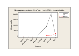
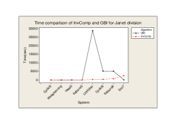
Figure 1: Comparison of InvComp and GBI for Janet division

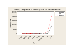
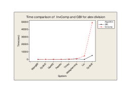
Figure 2: Comparison of InvComp and GBI for $\succ_{\mathop{\mathrm{alex}}\nolimits}$-division

It should be noted that the above presented experimental analysis of our new involutive completion algorithm InvComp is underdrawn. One needs to implement it efficiently either in Maple and compare with implementation of the GBI algorithm done in [17] or in C/C++ and compare with the GINV software [21]. In the last case the choice of heuristically good selection strategy [20] for a nonmultiplicative polongation to be processed (cf. line 5 in algorithm InvBase) and the use of proper data structures for the fast search of an involutive divisor [18] play a key role for the efficiency of involutive bases computation. As it was demonstrated by Faugère [12, 13], another very important source for computational efficiency of Gröbner bases algorithms is a clever use of linear algebra for performing reductions. We believe that this is applies equally to the involutive algorithms. Experimental comparison of GINV and another GBI implementation (JB) with Magma, Singular and accessible implementations of signature-based algorithms which do not exploit linear algebra is given on the Web page http://cag.jinr.ru/wiki/Benchmarking_for_polynomial_ideals.

References

- [1] J. Apel. Theory of involutive divisions and an application to Hilbert function computations. J. Symb. Comput., 25(6), 683–704, 1998.
- [2] J. Apel and R. Hemmecke. Detecting unnecessary reductions in an involutive basis computation. J. Symb. Comput., 40(4-5), 1131–1149, 2005.
- [3] G. Ars and A. Hashemi. Extended F5 criteria. J. Symb. Comput., 45(12), 1330–1340, 2010.
- [4] T. Becker and V. Weispfenning. Gröbner bases: a computational approach to commutative Algebra. Springer-Verlag, New York, 1993.
-
[5]
D. Bini and B. Mourrain.
Polynomial test suite.
http://www-sop.inria.fr/saga/POL/. - [6] B. Buchberger. Ein Algorithms zum Auffinden der Basiselemente des Restklassenrings nach einem nuildimensionalen Polynomideal. PhD Dissertation, Universität Innsbruck, 1965.
- [7] B. Buchberger. A criterion for detecting unnecessary reductions in the construction of Gröbner bases. Lect. Notes Comput. Sci. Springer, Berlin, 72, pp. 3–21, 1979.
- [8] B. Buchberger and F. Winkler, editors. Gröbner bases and applications, London Math. Society Lecture Note Series, 251. Cambridge University Press, Cambridge, 1998.
- [9] D. Cox, J. Little and D. O’Shea. Using algebraic geometry. 2nd Edition. Graduate Texts in Mathematics, 185. Springer, New York, 2005.
- [10] C. Eder and J. Perry. F5C: a variant of Faugère’s F5 algorithm with reduced Gröbner bases. J. Symb. Comput., 45(12), 1442–1458, 2010.
- [11] C. Eder and J. Perry. Signature-based algorithms to compute Gröbner bases. In: Proc. of ISSAC’11. ACM Press, pp. 99–106, 2011.
- [12] J.-C. Faugère. A new efficient algorithm for computing Gröbner bases . J. Pure Appl. Algebra, 139(1-3), 61–88, 1999.
- [13] J.-C. Faugère. A new efficient algorithm for computing Gröbner bases without reduction to zero . In: Proc. ISSAC’02. ACM Press, pp. 75–83, 2002.
- [14] S. Gao, Y. Guan and F. Volny IV. A new incremental algorithm for computing Groebner bases. In: Proc. ISSAC’10. ACM Press, pp. 13–19, 2010.
- [15] S. Gao, F. Volny IV and M. Wang. A new algorithm for computing Gröbner bases. Preprint, 2010. http://www.math.clemson.edu/sgao/pub.html
- [16] R. Gebauer and H. Möller. On an installation of Buchberger’s algorithm. J. Symb. Comput., 6(2-3), 275–286, 1988.
- [17] Y. A. Blinkov, V. P. Gerdt, C. F. Cid, W. Plesken and D. Robertz. The Maple package ”Janet”: I. Polynomial systems and II. Linear partial differential equations. Computer Algebra in Scientific Computing / CASC 2003, V. G. Ganzha, E. W. Mayr, and E. V. Vorozhtsov, eds. Institute of Informatics, Technical University of Munich, Garching, 2003, pp.31–54.
- [18] V. P. Gerdt. Involutive algorithms for computing Gröbner bases. Computational Commutative and Non-Commutative Algebraic Geometry, S. Cojocaru, G. Pfister and V. Ufnarovski, eds. Amstrerdam: IOS, pp. 199–225, 2005. (arXiv:math.AC/0501111)
- [Gerdt (2002)] V. P. Gerdt. On an algorithmic optimization in computation of involutive bases. Program. Comput. Soft., 28(2), 62–65, 2002.
- [19] V. P. Gerdt and Yu. A. Blinkov. Involutive bases of polynomial ideals. Math. Comput. Simulat., 45, 519–542, 1998; Minimal involutive bases. ibid., 543–560.
- [20] V. P. Gerdt and Yu. A. Blinkov. On selection of nonmultiplicative prolongations in computation of Janet bases. Program. Comput. Soft., 33(3), 147–153, 2007.
- [21] V. P. Gerdt and Yu. A. Blinkov. Specialized computer algebra system GINV. Program. Comput. Soft., 34, 112–123, 2008.
- [22] V. P. Gerdt and Yu. A. Blinkov. Involutive Division Generated by an Antigraded Monomial Ordering. Lect. Notes Comput. Sci., 6885. Springer, Berlin, pp.158–174, 2011.
- [23] V. P. Gerdt and D. A. Yanovich. Effectiveness of involutive criteria in computation of polynomial Janet bases. Program. Comput. Soft., 32, 134–138, 2006.
- [24] L. Huang. A new conception for computing Gröbner basis and its applications. arXiv:math.SC/1012.5424, 2010.
-
[25]
M. Janet.
Les systèmes d’équations aux dérivées partielles.
Journal de Mathématique, 3, 65–151, 1920. - [26] D. Lazard. Gröbner bases, Gaussian elimination and resolution of systems of algebraic equations. Lect. Notes Comput. Sci., 162. Springer, Berlin, pp. 146–156, 1983.
- [27] H. M. Möller, F. Mora and C. Traverso. Gröbner bases computation using syzygies. In: Proc.ISSAC’92. ACM Press, pp. 320–328, 1992.
- [28] T. Mora. Solving polynomial equation systems II. Macaulay’s paradigm and Gröbner technology. Encyclopedia of Mathematics and Its Applications, 99. Cambridge University Press, Cambridge, 2005.
- [29] S. Pan, Y. Hu and B. Wang. The termination of algorithms for computing Gröbner Bases. arXiv:math.AC/1202.3524, 2012.
- [30] V. Galkin. Termination of original F5. arXiv:math.AC/1203.2402, 2012.
- [31] J.-F. Pommaret. Systems of partial differential equations and Lie pseudogroups. Mathematics and its Applications, 14. Gordon & Breach Science Publishers, New York, 1978.
- [32] W. M. Seiler. Involution - The formal theory of differential equations and its applications in computer algebra. Springer-Verlag, Berlin Heidelberg, 2010.
- [33] Y. Sun and D. Wang. A generalized criterion for signature related Gröbner basis algorithms In: Proc. of ISSAC’11, ACM Press, pp. 337–344, 2011.
- [34] Y. Sun and D. Wang. The F5 algorithm in Buchberger’s style J. Syst. Sci . Complex., 24(6), 1218–1231, 2011.
- [35] J. Thomas. Differential systems. American Mathematical Society, New York, 1937.
- [36] A. Yu. Zharkov and Yu. A. Blinkov. Involutive approach to investigating polynomial systems. Math. Comput. Simulat., 42, 323–332, 1996.