Simultaneous Discrimination Prevention and Privacy Protection
in Data Publishing and Mining

SIMULTANEOUS DISCRIMINATION PREVENTION AND PRIVACY PROTECTION
IN DATA PUBLISHING AND MINING

A DISSERTATION
SUBMITTED TO THE DEPARTMENT OF COMPUTER ENGINEERING AND MATHEMATICS
OF UNIVERSITAT ROVIRA I VIRGILI
IN PARTIAL FULFILLMENT OF THE REQUIREMENTS
FOR THE DEGREE OF
DOCTOR OF PHILOSOPHY IN COMPUTER SCIENCE

© Copyright by Sara Hajian 2024
All Rights Reserved

I certify that I have read this dissertation and that, in my opinion, it is fully adequate in scope and quality as a dissertation for the degree of Doctor of Philosophy, and that it fulfils all the requirements to be eligible for the European Doctorate Award.

  Prof. Dr. Josep Domingo-Ferrer (Advisor)

I certify that I have read this dissertation and that, in my opinion, it is fully adequate in scope and quality as a dissertation for the degree of Doctor of Philosophy, and that it fulfils all the requirements to be eligible for the European Doctorate Award.

  Prof. Dr. Dino Pedreschi (Co-advisor)

Approved by the University Committee on Graduate Studies:

 

Abstract

Data mining is an increasingly important technology for extracting useful knowledge hidden in large collections of data. There are, however, negative social perceptions about data mining, among which potential privacy violation and potential discrimination. The former is an unintentional or deliberate disclosure of a user profile or activity data as part of the output of a data mining algorithm or as a result of data sharing. For this reason, privacy preserving data mining has been introduced to trade off the utility of the resulting data/models for protecting individual privacy. The latter consists of treating people unfairly on the basis of their belonging to a specific group. Automated data collection and data mining techniques such as classification have paved the way to making automated decisions, like loan granting/denial, insurance premium computation, etc. If the training datasets are biased in what regards discriminatory attributes like gender, race, religion, etc., discriminatory decisions may ensue. For this reason, anti-discrimination techniques including discrimination discovery and prevention have been introduced in data mining. Discrimination can be either direct or indirect. Direct discrimination occurs when decisions are made based on discriminatory attributes. Indirect discrimination occurs when decisions are made based on non-discriminatory attributes which are strongly correlated with biased discriminatory ones.

In the first part of this thesis, we tackle discrimination prevention in data mining and propose new techniques applicable for direct or indirect discrimination prevention individually or both at the same time. We discuss how to clean training datasets and outsourced datasets in such a way that direct and/or indirect discriminatory decision rules are converted to legitimate (non-discriminatory) classification rules. The experimental evaluations demonstrate that the proposed techniques are effective at removing direct and/or indirect discrimination biases in the original dataset while preserving data quality.

In the second part of this thesis, by presenting samples of privacy violation and potential discrimination in data mining, we argue that privacy and discrimination risks should be tackled together. We explore the relationship between privacy preserving data mining and discrimination prevention in data mining to design holistic approaches capable of addressing both threats simultaneously during the knowledge discovery process. As part of this effort, we have investigated for the first time the problem of discrimination and privacy aware frequent pattern discovery, i.e. the sanitization of the collection of patterns mined from a transaction database in such a way that neither privacy-violating nor discriminatory inferences can be inferred on the released patterns. Moreover, we investigate the problem of discrimination and privacy aware data publishing, i.e. transforming the data, instead of patterns, in order to simultaneously fulfill privacy preservation and discrimination prevention. In the above cases, it turns out that the impact of our transformation on the quality of data or patterns is the same or only slightly higher than the impact of achieving just privacy preservation.

To my family, advisors and friends

Contents

1. Abstract
2. 1 Introduction
   1. 1.1 Privacy Challenges of Data Publishing and Mining
   2. 1.2 Discrimination Challenges of Data Publishing and Mining
   3. 1.3 Simultaneous Discrimination Prevention and Privacy Protection in Data Publishing and Mining
      1. 1.3.1 Contributions
      2. 1.3.2 Structure
3. 2 Background on Discrimination-aware Data Mining
   1. 2.1 Related Work
      1. 2.1.1 Discrimination Discovery from Data
      2. 2.1.2 Discrimination Prevention in Data Mining
   2. 2.2 Preliminaries
      1. 2.2.1 Basic Definitions
      2. 2.2.2 Measures of Discrimination
4. 3 Background on Privacy-aware Data Mining
   1. 3.1 Brief Review
   2. 3.2 Preliminaries
      1. 3.2.1 Basic Definitions
      2. 3.2.2 Models of Privacy
      3. 3.2.3 Sanitization Mechanisms
   3. 3.3 Approaches and Algorithms
      1. 3.3.1 Privacy Preserving Data Publishing
      2. 3.3.2 Privacy Preserving Knowledge Publishing
5. 4 A Methodology for Direct and Indirect Discrimination Prevention in Data Mining
   1. 4.1 Contributions
   2. 4.2 Direct and Indirect Discrimination Measurement
   3. 4.3 The Approach
   4. 4.4 Data Transformation for Direct Discrimination
      1. 4.4.1 Direct Rule Protection (DRP)
      2. 4.4.2 Rule Generalization (RG)
      3. 4.4.3 Direct Rule Protection and Rule Generalization
   5. 4.5 Data Transformation for Indirect Discrimination
      1. 4.5.1 Indirect Rule Protection (IRP)
   6. 4.6 Data Transformation for Both Direct and Indirect Discrimination
   7. 4.7 The Algorithms
      1. 4.7.1 Direct Discrimination Prevention Algorithms
      2. 4.7.2 Indirect Discrimination Prevention Algorithms
      3. 4.7.3 Direct and Indirect Discrimination Prevention Algorithms
   8. 4.8 Computational Cost
   9. 4.9 Experiments
      1. 4.9.1 Datasets
      2. 4.9.2 Utility Measures
      3. 4.9.3 Empirical Evaluation
   10. 4.10 Conclusions
6. 5 Discrimination- and Privacy-aware Frequent Pattern Discovery
   1. 5.1 Introduction
      1. 5.1.1 Motivating Example
      2. 5.1.2 Contributions
   2. 5.2 Privacy-aware Frequent Pattern Discovery
      1. 5.2.1 Anonymous Frequent Pattern Set
      2. 5.2.2 Achieving an Anonymous Frequent Pattern Set
   3. 5.3 Discrimination-aware Frequent Pattern Discovery
      1. 5.3.1 Discrimination Protected Frequent Pattern Set
      2. 5.3.2 Unexplainable Discrimination Protected Frequent Pattern Set
      3. 5.3.3 Achieving a Discrimination Protected Frequent Pattern Set
      4. 5.3.4 Achieving an Unexplainable Discrimination Protected Pattern Set
   4. 5.4 Simultaneous Discrimination-Privacy Awareness in Frequent Pattern Discovery
      1. 5.4.1 Achieving a Discrimination and Privacy Protected Frequent Pattern Set
      2. 5.4.2 Achieving an Unexplainable Discrimination and Privacy Protected Pattern Set
   5. 5.5 Experiments
      1. 5.5.1 Utility Measures
      2. 5.5.2 Empirical Evaluation
   6. 5.6 An Extension Based on Differential Privacy
      1. 5.6.1 Differentially Private Frequent Pattern Set
      2. 5.6.2 Achieving an Differentially Private Frequent Pattern Set
      3. 5.6.3 Achieving a Discrimination Protected and Differential Private Frequent Pattern Set
      4. 5.6.4 Discussion
   7. 5.7 Conclusions
7. 6 A Study on the Impact of Data Anonymization on Anti-discrimination
   1. 6.1 Non-discrimination Model
   2. 6.2 Data Anonymization Techniques and Anti-discrimination
      1. 6.2.1 Global Recoding Generalizations and Anti-discrimination
      2. 6.2.2 Local Recoding Generalizations and Anti-discrimination
      3. 6.2.3 Multidimensional Generalizations and Anti-discrimination
      4. 6.2.4 Suppression and Anti-discrimination
   3. 6.3 Conclusion
8. 7 Generalization-based Privacy Preservation and Discrimination Prevention in Data Publishing and Mining
   1. 7.1 Introduction
      1. 7.1.1 Motivating Example
      2. 7.1.2 Contributions
   2. 7.2 Privacy Model
   3. 7.3 Non-discrimination Model
   4. 7.4 Simultaneous Privacy Preservation and Discrimination Prevention
      1. 7.4.1 The Generalization-based Approach
      2. 7.4.2 The Algorithm
   5. 7.5 Experiments
      1. 7.5.1 Dataset
      2. 7.5.2 Performance
      3. 7.5.3 Data Quality
   6. 7.6 Extensions
      1. 7.6.1 Alternative Privacy Models
      2. 7.6.2 Alternative Anti-discrimination Legal Concepts
   7. 7.7 Conclusions
9. 8 Conclusions
   1. 8.1 Contributions
   2. 8.2 Publications
   3. 8.3 Future Work

List of Tables

1. 4.1 Data transformation methods (DTMs) for different measures
2. 4.2 Direct and indirect rule protection methods
3. 4.3 Adult dataset: Utility measures for minimum support 2% and confidence 10% for all the methods. Value “n.a.” denotes that the respective measure is not applicable.
4. 4.4 German Credit dataset: Utility measures for minimum support 5% and confidence 10% for all methods. Value “n.a.” denotes that the respective measure is not applicable.
5. 4.5 Adult dataset: Utility measures for minimum support 2% and confidence 10% for direct and indirect rule protection; columns show the results for different values of $\alpha$. Value “n.a.” denotes that the respective measure is not applicable.
6. 4.6 German Credit dataset: Utility measures for minimum support 5% and confidence 10% for direct and indirect rule protection; columns show the results for different values of $\alpha$. Value “n.a.” denotes that the respective measure is not applicable.
7. 4.7 Adult dataset: number of frequent classification rules and $\alpha-$discriminatory rules found during the tests, for minimum confidence 10% and different values of minimum support (2%, 5% and 10%)
8. 4.8 Adult dataset: utility measures for minimum confidence 10%, $\alpha$=1.2 and $d=0.9$; columns show the results for different values of minimum support (2%, 5% and 10%) and different methods.
9. 5.1 A data table of personal decision records
10. 5.2 Scenario 1: Examples of frequent patterns extracted from Table 5.1
11. 5.3 Scenario 2: Examples of frequent patterns extracted from Table 5.1
12. 5.4 Scenario 3: Examples of frequent patterns extracted from Table 5.1
13. 5.5 Scenario 4: Examples of frequent patterns extracted from Table 5.1
14. 5.6 Adult dataset: accuracy of classifiers
15. 5.7 German dataset: accuracy of classifiers
16. 5.8 Discrimination utility measures after privacy pattern sanitization: Adult (top); German credit (bottom)
17. 5.9 Percentage of $d$-explainable patterns detected in $\mathcal{FP}$ and $\mathcal{FP}^{\prime}$
18. 6.1 Private data table with biased decision records
19. 6.2 Different types of cell generalization
20. 6.3 Different types of record suppression
21. 6.4 Summary of results
22. 7.1 Private data set with biased decision records
23. 7.2 Description of the Adult data set

List of Figures

1. 2.1 Discrimination measures
2. 3.1 Generalization taxonomy tree for Sex, Job and Age attributes
3. 4.1 The process of extracting biased and unbiased decision rules
4. 4.2 Information loss (left) and discrimination removal degree (right) for direct discrimination prevention methods for $\alpha\in[1.2,1.7]$. DRP(Method $i$): Method $i$ for DRP; RG: Rule Generalization.
5. 4.3 Information loss (left) and discrimination removal (right) degree for direct discrimination prevention methods for $d\in[0.8,0.95]$. DRP(Method$i$): Method $i$ for DRP; RG: Rule Generalization.
6. 4.4 Execution times (left) and Information loss degree (right) of Method 1 for DRP for $\alpha\in[1.2,1.7]$ with and without impact minimization.
7. 4.5 Adult dataset: Information loss (left) and discrimination removal degree (right) for discrimination prevention methods for minimum support=2%, $\alpha=1.2$, $p=0.9$ and minimum confidence in $[10,90]$. DRP(Method $i$): Method $i$ for DRP; RG: Rule Generalization.
8. 5.1 Pattern distortion scores to make the Adult dataset $k$-anonymous
9. 5.2 Pattern distortion scores to make the German credit dataset $k$-anonymous
10. 5.3 Pattern distortion scores to make the Adult dataset $\alpha$-protective
11. 5.4 Pattern distortion scores to make the German dataset $\alpha$-protective
12. 5.5 Pattern distortion scores to make the Adult dataset $\alpha$-protective $k$-anonymous
13. 5.6 Pattern distortion scores to make the German dataset $\alpha$-protective $k$-anonymous
14. 7.1 An example of domain (left) and value (right) generalization hierarchies of Race, Sex and Hours attributes
15. 7.2 Generalization lattice for the Race and Sex attributes
16. 7.3 The candidate 1- and 2-attribute generalization of Table 7.1 by Incognito(left) and $\alpha$-protective Incognito (right)
17. 7.4 Performance of Incognito and $\alpha$-protective Incognito for several values of $k$, $\tau$, $f$ and $DA$. Unless otherwise specified, $f=slift$ , $DA=DA_{1}$ and $\tau=4$.
18. 7.5 General data quality metrics. Left, generalization height (GH). Right, discernibility ratio (DR). Results are given for $k$-anonymity (I); and $\alpha$-protection $k$-anonymity with $DA_{3}$, $\alpha=1.2$ (II); $DA_{3}$, $\alpha=1.6$ (III); $DA_{1}$, $\alpha=1.2$ (IV); $DA_{1}$, $\alpha=1.6$ (V). In all cases $f=slift$.
19. 7.6 Data quality for classification analysis Left, classification metric (CM). Right, classification accuracy, in percentage (CA). Results are given for the original data (0); $k$-anonymity (I); and $\alpha$-protection $k$-anonymity with $DA_{3}$, $\alpha=1.2$ (II); $DA_{3}$, $\alpha=1.6$ (III); $DA_{1}$, $\alpha=1.2$ (IV); $DA_{1}$, $\alpha=1.6$ (V). In all cases $f=slift$.

Chapter 1 Introduction

Data mining is an increasingly important technology for extracting useful knowledge hidden in large collections of data, especially human and social data sensed by the ubiquitous technologies that support most human activities in our age. As a matter of fact, the new opportunities to extract knowledge and understand human and social complex phenomena increase hand in hand with the risks of violation of fundamental human rights, such as privacy and non-discrimination. Privacy refers to the individual right to choose freely what to do with one’s own personal information, while discrimination refers to unfair or unequal treatment of people based on membership to a category, group or minority, without regard to individual merit. Human rights laws not only have concern about data protection [21] but also prohibit discrimination [6, 22] against protected groups on the grounds of race, color, religion, nationality, sex, marital status, age and pregnancy; and in a number of settings, like credit and insurance, personnel selection and wages, and access to public services. Clearly, preserving the great benefits of data mining within a privacy-aware and discrimination-aware technical ecosystem would lead to a wider social acceptance of a multitude of new services and applications based on the knowledge discovery process.

1.1 Privacy Challenges of Data Publishing and Mining

We live in times of unprecedented opportunities of sensing, storing and analyzing micro-data on human activities at extreme detail and resolution, at society level [67]. Wireless networks and mobile devices record the traces of our movements. Search engines record the logs of our queries for finding information on the web. Automated payment systems record the tracks of our purchases. Social networking services record our connections to friends, colleagues, collaborators.

Ultimately, these big data of human activity are at the heart of the very idea of a knowledge society [67]: a society where small or big decisions made by businesses or policy makers or ordinary citizens – can be informed by reliable knowledge, distilled from the ubiquitous digital traces generated as a side effect of our living. Although increasingly sophisticated data analysis and data mining techniques support knowledge discovery from human activity data to improve the quality of on-line and off-line services for users, they are increasingly raising user privacy concerns on the other side.

From the users’ perspective, insufficient privacy protections on the part of a service they use and entrust with their activity, personal or sensitive information could lead to significant emotional, financial, and physical harm. An unintentional or deliberate disclosure of a user profile or activity data as part of the output of an internal data mining algorithm or as a result of data sharing may potentially lead to embarrassment, identity theft and discrimination [48]. It is hard to foresee all the privacy risks that a digital dossier consisting of detailed profile and activity data could pose in the future, but it is not inconceivable that it could harm users’ lives. In general, during knowledge discovery, privacy violation is an unintentional or deliberate intrusion into the personal data of the data subjects, namely, of the (possibly unaware) people whose data are being collected, analyzed and mined [67].

Thus, although users appreciate the continual innovation and improvement in the quality of on-line and off-line services using sophisticated data analysis and mining techniques, they are also becoming increasingly concerned about their privacy, and about the ways their personal and activity data are compiled, mined, and shared [72]. On the other hand, for institutions and companies such as banks, insurance companies and search engines that offer different kinds of online and/or off-line services, the trust of users in their privacy practices is a strategic product and business advantage. Therefore, it is in the interest of these organizations to strike a balance between mining and sharing user data in order to improve their services and protecting user privacy to retain the trust of users [86].

In order to respond to the above challenges, data protection technology needs to be developed in tandem with data mining and publishing techniques [87]. The framework to advance is thinking of privacy by design. The basic idea is to inscribe privacy protection into the analytical technology by design and construction, so that the analysis takes the privacy requirements in consideration from the very start. Privacy by design, in the research field of privacy preserving data mining (PPDM), is a recent paradigm that promises a quality leap in the conflict between data protection and data utility. PPDM has become increasingly popular because it allows sharing and using sensitive data for analysis purposes. Different PPDM methods have been developed for different purposes, such as data hiding, knowledge (rule) hiding, distributed PPDM and privacy-aware knowledge sharing in different data mining tasks.

1.2 Discrimination Challenges of Data Publishing and Mining

Discrimination refers to an unjustified difference in treatment on the basis of any physical or cultural trait, such as sex, ethnic origin, religion or political opinions. From the legal perspective, privacy violation is not the only risk which threatens fundamental human rights; discrimination risks are also concerned when mining and sharing personal data. In most European and North-American countries, it is forbidden by law to discriminate against certain protected groups [11]. The European Union has one of the strongest anti-discrimination legislations (See, e.g., Directive 2000/43/EC, Directive 2000/78/EC/ Directive 2002/73/EC, Article 21 of the Charter of Fundamental Rights and Protocol 12/Article 14 of the European Convention on Human Rights), describing discrimination on the basis of race, ethnicity, religion, nationality, gender, sexuality, disability, marital status, genetic features, language and age. It does so in a number of settings, such as employment and training, access to housing, public services, education and health care; credit and insurance; and adoption. European efforts on the non-discrimination front make clear the fundamental importance of the effective implementation and enforcement of non-discrimination norms [11] for Europe’s citizens.

From the user’s perspective, many people may not mind other people knowing about their ethnic origins, but they would strenuously object to be denied a credit or a grant if their ethnicities were part of that decision. As mentioned above, nowadays socially sensitive decisions may be taken by automatic systems, e.g., for screening or ranking applicants to a job position, to a loan, to school admission and so on. For instance, data mining and machine learning classification models are constructed on the basis of historical data exactly with the purpose of learning the distinctive elements of different classes or profiles, such as good/bad debtor in credit/insurance scoring systems. Automatically generated decision support models may exhibit discriminatory behavior toward certain groups based upon, e.g. gender or ethnicity. In general, during knowledge discovery, discrimination risk is the unfair use of the discovered knowledge in making discriminatory decisions about the (possibly unaware) people who are classified, or profiled [67]. Therefore, it is in the interest of banks, insurance companies, employment agencies, the police and other institutions that employ data mining models for decision making upon individuals, to ensure that these computational models are free from discrimination [11].

Then, data mining and data analytics on data about people need to incorporate many ethical values by design, not only data protection but also non-discrimination. We need novel, disruptive technologies for the construction of human knowledge discovery systems that, by design, offer native technological safeguards against discrimination. Anti-discrimination by design, in the research field of discrimination prevention in data mining (DPDM), is a more recent paradigm that promises a quality leap in the conflict between non-discrimination and data/model utility. More specifically, discrimination has been recently considered from a data mining perspective. Some proposals are oriented to the discovery and measurement of discrimination, while others deal with preventing data mining from becoming itself a source of discrimination, due to automated decision making based on discriminatory models extracted from biased datasets. In fact, DPDM consists of extracting models (typically, classifiers) that trade off utility of the resulting data/model with non-discrimination.

1.3 Simultaneous Discrimination Prevention and Privacy Protection in Data Publishing and Mining

In this thesis, by exploring samples of privacy violation and discrimination risks in contexts of data and knowledge publishing, we realize that privacy and anti-discrimination are two intimately intertwined concepts: they share common challenges, common methodological problems to be solved and, in certain contexts, directly interact with each other. Despite this striking commonality, there is an evident gap between the large body of research in data privacy technologies and the recent early results in anti-discrimination technologies. This thesis aims to answer the following research questions:

• What is the relationship between PPDM and DPDM? Can privacy protection achieve anti-discrimination (or the other way round)?

• Can we adapt and use some of the existing approaches from the PPDM literature for DPDM?

• Is it enough to tackle only privacy or discrimination risks to make a truly trustworthy technology for knowledge discovery? If not, how can we design a holistic method capable of addressing both threats together in significant data mining processes?

This thesis aims to find ways to mine and share personal data while protecting users’ privacy and preventing discrimination against protected groups of users, and to motivate companies, institutions and the research community to consider a need for simultaneous privacy and anti-discrimination by design. This thesis is the first work inscribing simultaneously privacy and anti-discrimination with a by design approach in data publishing and mining. It is a first example of a more comprehensive set of ethical values that is inscribed into the analytical process.

1.3.1 Contributions

Specifically, this thesis makes the following concrete contributions to answer the above questions:

1. A methodology for direct and indirect discrimination prevention in data mining. We tackle discrimination prevention in data mining and propose new techniques applicable for direct or indirect discrimination prevention individually or both at the same time. Inspired by the data transformation methods for knowledge (rule) hiding in PPDM, we devise new data transformation methods (i.e. direct and indirect rule protection, rule generalization) for converting direct and/or indirect discriminatory decision rules to legitimate (non-discriminatory) classification rules. We also propose new metrics to evaluate the utility of the proposed approaches and we compare these approaches. The experimental evaluations demonstrate that the proposed techniques are effective at removing direct and/or indirect discrimination biases in the original dataset while preserving data quality.

2. Discrimination- and privacy-aware frequent pattern discovery. Consider the case when a set of patterns extracted from the personal data of a population of individual persons is released for a subsequent use into a decision making process, such as granting or denying credit. First, the set of patterns may reveal sensitive information about individual persons in the training population and, second, decision rules based on such patterns may lead to unfair discrimination, depending on what is represented in the training cases. We argue that privacy and discrimination risks should be tackled together, and we present a methodology for doing so while publishing frequent pattern mining results. We describe a set of pattern sanitization methods, one for each discrimination measure used in the legal literature, to achieve a fair publishing of frequent patterns in combination with a privacy transformation based on $k$-anonymity. Our proposed pattern sanitization methods yield both privacy- and discrimination-protected patterns, while introducing reasonable (controlled) pattern distortion. We also explore the possibility to combine anti-discrimination with differential privacy.

3. Generalization-based privacy preservation and discrimination prevention in data publishing. We investigate the problem of discrimination and privacy aware data publishing, i.e. transforming the data, instead of patterns, in order to simultaneously fulfill privacy preservation and discrimination prevention. Our approach falls into the pre-processing category: it sanitizes the data before they are used in data mining tasks rather than sanitizing the knowledge patterns extracted by data mining tasks (post-processing). Very often, knowledge publishing (publishing the sanitized patterns) is not enough for the users or researchers, who want to be able to mine the data themselves. This gives researchers greater flexibility in performing the required data analyses. We observe that published data must be both privacy-preserving and unbiased regarding discrimination. We present the first generalization-based approach to simultaneously offer privacy preservation and discrimination prevention. We formally define the problem, give an optimal algorithm to tackle it and evaluate the algorithm in terms of both general and specific data analysis metrics. It turns out that the impact of our transformation on the quality of data is the same or only slightly higher than the impact of achieving just privacy preservation. In addition, we show how to extend our approach to different privacy models and anti-discrimination legal concepts.

The presentation of this thesis is divided into eight chapters according to the contributions.

1.3.2 Structure

This thesis is organized as follows. In Chapter 2, we review the related works on discrimination discovery and prevention in data mining (Section 2.1). Moreover, we introduce some basic definitions and concepts that are used throughout this thesis related to data mining (Section 2.2.1) and measures of discrimination (Section 2.2.2). In Chapter 3, we first present a brief review on PPDM in Section 3.1. After that, we introduce some basic definitions and concepts that are used throughout the thesis related to data privacy (Section 3.2.1), and we elaborate on models (measures) of privacy (Section 3.2.2) and samples of anonymization techniques (Section 3.2.3). Finally, we review the approaches and algorithms of PPDM in Section 3.3.

In Chapter 4, we propose a methodology for direct and indirect discrimination prevention in data mining. Our contributions on discrimination prevention are presented in Section 4.1. Section 4.2 introduces direct and indirect discrimination measurement. Section 4.3 describes our proposal for direct and indirect discrimination prevention. The proposed data transformation methods for direct and indirect discrimination prevention are presented in Section 4.4 and Section 4.5, respectively. Section 4.6 introduces the proposed data transformation methods for simultaneous direct and indirect discrimination prevention. We describe our algorithms and their computational cost based on the proposed direct and indirect discrimination prevention methods in Section 4.7 and Section 4.8, respectively. Section 4.9 shows the tests we have performed to assess the validity and quality of our proposal and we compare different methods. Finally, Section 4.10 summarizes conclusions.

In Chapter  5, we propose the first approach for achieving simultaneous discrimination and privacy awareness in frequent pattern discovery. Section 5.1 presents the motivation example (Section 5.1.1) and our contributions (Section 5.1.2) in frequent pattern discovery. Section 5.2 presents the method that we use for obtaining an anonymous version of an original pattern set. Section 5.3 describes the notion of discrimination protected (Section 5.3.1) and unexplainable discrimination protected (Section 5.3.2) frequent patterns. Then, our proposed methods and algorithms to obtain these pattern sets are presented in Sections 5.3.3 and 5.3.4, respectively. In Section 5.4, we formally define the problem of simultaneous privacy and anti-discrimination pattern protection, and we introduce our solution. Section 5.5 reports the evaluation of our sanitization methods. In Section 5.6, we study and discuss the use of a privacy protection method based on differential privacy and its implications. Finally, Section 5.7 concludes the chapter.

In Chapter 6, we present a study on the impact of well-known data anonymization techniques on anti-discrimination. Our proposal for releasing discrimination-free version of original data is presented in Section 6.1. In Section 6.2, we study the impact of different generalization and suppression schemes on discrimination prevention. Finally, Section 6.3 summarizes conclusions. In Chapter 7, we present a generalization-based approach for privacy preservation and discrimination prevention in data publishing. Privacy and anti-discrimination models are presented in Section 7.2 and 7.3, respectively. In Section 7.4, we formally define the problem of simultaneous privacy and anti-discrimination data protection. Our proposed approach and an algorithm for discrimination- and privacy-aware data publishing are presented in Sections 7.4.1 and 7.4.2. Section 7.5 reports experimental work. An extension of the approach to alternative privacy-preserving requirements and anti-discrimination legal constraints is presented in Section 7.6. Finally, Section 7.7 summarizes conclusions.

Finally, Chapter 8 is the closing chapter. It briefly recaps the thesis contributions, it lists the publications that have resulted from our work, it states some conclusions and it identifies open issues for future work.

Chapter 2 Background on Discrimination-aware Data Mining

In sociology, discrimination is the prejudicial treatment of an individual based on their membership in a certain group or category. It involves denying to members of one group opportunities that are available to other groups. There is a list of anti-discrimination acts, which are laws designed to prevent discrimination on the basis of a number of attributes (e.g. race, religion, gender, nationality, disability, marital status and age) in various settings (e.g. employment and training, access to public services, credit and insurance, etc.). For example, the European Union implements in [23] the principle of equal treatment between men and women in the access to and supply of goods and services; also, it implements equal treatment in matters of employment and occupation in [24]. Although there are some laws against discrimination, all of them are reactive, not proactive. Technology can add proactivity to legislation by contributing discrimination discovery and prevention techniques.

2.1 Related Work

The collection and analysis of observational and experimental data are the main tools for assessing the presence, the extent, the nature, and the trend of discrimination phenomena. Data analysis techniques have been proposed in the last fifty years in the economic, legal, statistical, and, recently, in data mining literature. This is not surprising, since discrimination analysis is a multi-disciplinary problem, involving sociological causes, legal argumentations, economic models, statistical techniques, and computational issues. For a multidisciplinary survey on discrimination analysis see [75]. In this thesis, we focus on a knowledge discovery (or data mining) perspective of discrimination analysis.

Recently, the issue of anti-discrimination has been considered from a data mining perspective [68], under the name of discrimination-aware data analysis. A substantial part of the existing literature on anti-discrimination in data mining is oriented to discovering and measuring discrimination. Other contributions deal with preventing discrimination. Summaries of contributions in discrimination-aware data analysis are collected in [14].

2.1.1 Discrimination Discovery from Data

Unfortunately, the actual discovery of discriminatory situations and practices, hidden in a dataset of historical decision records, is an extremely difficult task. The reason is twofold:

• First, personal data in decision records are typically highly dimensional: as a consequence, a huge number of possible contexts may, or may not, be the theater for discrimination. To see this point, consider the case of gender discrimination in credit approval: although an analyst may observe that no discrimination occurs in general, it may turn out that older women obtain car loans only rarely. Many small or large niches that conceal discrimination may exist, and therefore all possible specific situations should be considered as candidates, consisting of all possible combinations of variables and variable values: personal data, demographics, social, economic and cultural indicators, etc. The anti-discrimination analyst is thus faced with a combinatorial explosion of possibilities, which make her work hard: albeit the task of checking some known suspicious situations can be conducted using available statistical methods and known stigmatized groups, the task of discovering niches of discrimination in the data is unsupported.

• The second source of complexity is indirect discrimination: the feature that may be the object of discrimination, e.g., the race or ethnicity, is not directly recorded in the data. Nevertheless, racial discrimination may be hidden in the data, for instance in the case where a redlining practice is adopted: people living in a certain neighborhood are frequently denied credit, but from demographic data we can learn that most people living in that neighborhood belong to the same ethnic minority. Once again, the anti-discrimination analyst is faced with a large space of possibly discriminatory situations: all interesting discriminatory situations that emerge from the data, both directly and in combination with further background knowledge need to be discovered (e.g., census data).

Pedreschi et al. [68, 69, 77, 70] have introduced the first data mining approaches for discrimination discovery. The approaches have followed the legal principle of under-representation to unveil contexts of possible discrimination against protected-by-law groups (e.g., women). This is done by extracting classification rules from a dataset of historical decision records (inductive part); then, rules are ranked according to some legally grounded measures of discrimination (deductive part). The approach has been implemented on top of an Oracle database [76] by relying on tools for frequent itemset mining. A GUI for visual exploratory analysis has been developed by Gao and Berendt in [30].

This discrimination discovery approach opens a promising avenue for research, based on an apparently paradoxical idea: data mining, that has a clear potential to create discriminatory profiles and classifications, can also be used the other way round, as a powerful aid to the anti-discrimination analyst, capable of automatically discovering the patterns of discrimination that emerge from the available data with strongest evidence.

The result of the above knowledge discovery process is a (possibly large) set of classification rules, which provide local and overlapping niches of possible discrimination: a global description is lacking of who is and is not discriminated against. Luong et al. [60] exploit the idea of situation-testing. For each member of the protected group with a negative decision outcome, testers with similar characteristics are searched for in a dataset of historical decision records. If there are significantly different decision outcomes between the testers of the protected group and the testers of the unprotected group, the negative decision can be ascribed to a bias against the protected group, thus labeling the individual as discriminated against. Similarity is modeled via a distance function. Testers are searched for among the $k$-nearest neighbors, and the difference is measured by some legally grounded measures of discrimination calculated over the two sets of testers. After this kind of labeling, a global description of those labeled as discriminated against can be extracted as a standard classification task. A real case study in the context of the evaluation of scientific projects for funding is presented by Romei et al. [74].

The approaches described so far assume that the dataset under analysis contains attributes that denote protected groups (i.e., case of direct discrimination). This may not be the case when such attributes are not available, or not even collectable at a micro-data level (i.e., case of indirect discrimination), as in the case of the loan applicant’s race. Ruggieri et al. [70, 77] adopt a form of rule inference to cope with the indirect discovery of discrimination. The correlation information is called background knowledge, and is itself coded as an association rule.

The above results do not yet explain how to build a discrimination-free knowledge discovery and deployment (KDD) technology for decision making. This is crucial as we are increasingly surrounded by automatic decision making software that makes decisions on people based on profiles and categorizations. We need novel, disruptive technologies for the construction of human knowledge discovery systems that, by design, offer native technological safeguards against discrimination. Here we evoke the concept of “Privacy by Design” coined in the ‟90s by Ann Cavoukian, the Information and Privacy Commissioner of Ontario, Canada. In brief, Privacy by Design refers to the philosophy and approach of embedding privacy into the design, operation and management of information processing technologies and systems.

In different contexts, adopting different techniques for inscribing discrimination protection within the KDD process will be needed, in order to go beyond the discovery of unfair discrimination, and achieve the much more challenging goal of preventing discrimination, before it takes place.

2.1.2 Discrimination Prevention in Data Mining

With the advent of data mining, decision support systems become increasingly intelligent and versatile, since effective decision models can be constructed on the basis of historical decision records by means of machine learning and data mining methods, up to the point that decision making is sometimes fully automated, e.g., in credit scoring procedures and in credit card fraud detection systems. However, there is no guarantee that the deployment of the extracted knowledge does not incur discrimination against minorities and disadvantaged groups, e.g., because the data from which the knowledge is extracted contain patterns with implicit discriminatory bias. Such patterns will then be replicated in the decision rules derived from the data by mining and learning algorithms. Hence, learning from historical data may lead to the discovery of traditional prejudices that are endemic in reality, and to assigning the status of general rules to such practices (maybe unconsciously, as these rules can end up deeply hidden within a piece of software).

Thus, beyond discrimination discovery, preventing knowledge-based decision support systems from making discriminatory decisions is a more challenging issue. A straightforward approach to avoid that the classifier’s prediction be based on the discriminatory attribute would be to remove that attribute from the training dataset. This approach, however, does not work [43, 11]. The reason is that there may be other attributes that are highly correlated with the discriminatory one. In such a situation the classifier will use these correlated attributes to indirectly discriminate. In the banking example, e.g., postal code may be highly correlated with ethnicity. Removing ethnicity would not solve much, as postal code is an excellent predictor for this attribute. Obviously, one could decide to also remove the highly correlated attributes from the dataset as well. Although this would resolve the discrimination problem, in this process much useful information will get lost, leading to suboptimal predictors [43, 11]. Hence, there are two important challenges regarding discrimination prevention: one challenge is to consider both direct and indirect discrimination instead of only direct discrimination; the other challenge is to find a good trade off between discrimination removal and the utility of the data/models for data mining. In such a context, the challenging problem of discrimination prevention consists of re-designing existing data publishing and knowledge discovery techniques in order to incorporate a legally grounded notion of non-discrimination in the extracted knowledge, with the objective that the deployment phase leads to non-discriminatory decisions. Up to now, four non mutually-exclusive strategies have been proposed to prevent discrimination in the data mining and knowledge discovery process.

The first strategy consists of a controlled distortion of the training set (a pre-processing approach). Kamiran and Calders [43] compare sanitization techniques such as changing class labels based on prediction confidence, instance re-weighting, and sampling. Zliobaitye et al. [97] prevent excessive sanitization by taking into account legitimate explanatory variables that are correlated with grounds of discrimination, i.e., genuine occupational requirement. The approach of Luong et al. [60] extends to discrimination prevention by changing the class label of individuals that are labeled as discriminated. The advantage of the pre-processing approach is that it does not require changing the standard data mining algorithms, unlike the in-processing approach, and it allows data publishing (rather than just knowledge publishing), unlike the post-processing approach.

The second strategy is to modify the classification learning algorithm (an in-processing approach), by integrating it with anti-discrimination criteria. Calders and Verwer [12] consider three approaches to deal with naive Bayes models, two of which consist in modifying the learning algorithm: training a separate model for each protected group; and adding a latent variable to model the class value in the absence of discrimination. Kamiran et al. [44] modify the entropy-based splitting criterion in decision tree induction to account for attributes denoting protected groups. Kamishima et al. [46] measure the indirect causal effect of variables modeling grounds of discrimination on the independent variable in a classification model by their mutual information. Then, they apply a regularization (i.e., a change in the objective minimization function) to probabilistic discriminative models, such as logistic regression.

The third strategy is to post-process the classification model once it has been extracted. Pedreschi et al. [69] alter the confidence of classification rules inferred by the CPAR algorithm. Calders and Verwer [12] act on the probabilities of a naive Bayes model. Kamiran et al. [44] re-label the class predicted at the leaves of a decision tree induced by C4.5. Finally, the fourth strategy assumes no change in the construction of a classifier. At the time of application, instead, predictions are corrected to keep proportionality of decisions among protected and unprotected groups. Kamiran et al. [45] propose correcting predictions of probabilistic classifiers that are close to the decision boundary, given that (statistical) discrimination may occur when there is no clear feature supporting a positive or a negative decision.

Moreover, on the relationship between privacy and anti-discrimination from legal perspective, the chapter by Gellert et al. [32] reports a comparative analysis of data protection and anti-discrimination legislations. And from the technology perspective, Dwork et al. [20] propose a model of fairness of classifiers and relate it to differential privacy in databases. The model imposes that the predictions over two similar cases be also similar. The similarity of cases is formalized by a distance measure between tuples. The similarity of predictions is formalized by the distance between the distributions of probability assigned to class values.

2.2 Preliminaries

In this section, we briefly review the background knowledge required in the remainder of this thesis. First, we recall some basic definitions related to data mining [84]. After that, we elaborate on measuring and discovering discrimination.

2.2.1 Basic Definitions

Let $\mathcal{I}=\{i_{1},\ldots,i_{n}\}$ be a set of items, where each item $i_{j}$ has the form attribute=value (e.g., Sex=female). An itemset $X\subseteq\mathcal{I}$ is a collection of one or more items, e.g. {Sex=female, Credit_history=no-taken}. A database is a collection of data objects (records) and their attributes; more formally, a (transaction) database $\mathcal{D}=\{r_{1},\ldots,r_{m}\}$ is a set of data records or transactions where each $r_{i}\subseteq\mathcal{I}$. Civil rights laws [6, 22] explicitly identify the groups to be protected against discrimination, such as minorities and disadvantaged people, e.g., women. In our context, these groups can be represented as items, e.g., Sex=female, which we call potentially discriminatory (PD) items; a collection of PD items can be represented as an itemset, e.g., {Sex=female, Foreign_worker=yes}, which we call PD itemset or protected-by-law (or protected for short) groups, denoted by $DI_{b}$. An itemset $X$ is potentially non-discriminatory (PND) if $X\cap DI_{b}=\emptyset$, e.g., {credit_history=no-taken} is a PND itemset where $DI_{b}$:{Sex=female}. PD attributes are those that can take PD items as values; for instance, Race and Gender where $DI_{b}$:{Sex=female, Race=black}. A decision (class) attribute is one taking as values yes or no to report the outcome of a decision made on an individual; an example is the attribute credit_approved, which can be yes or no. A class item is an item of class attribute, e.g., Credit_approved=no. The support of an itemset $X$ in a database $\mathcal{D}$ is the number of records that contain $X$, i.e. $supp_{\mathcal{D}}(X)=|\{r_{i}\in\mathcal{D}|X\subseteq r_{i}\}|$, where $|\ .\ |$ is the cardinality operator. From patterns, it is possible to derive association rules. An association rule is an expression $X\rightarrow Y$, where X and Y are itemsets. We say that $X\rightarrow Y$ is a classification rule if $Y$ is a class item and $X$ is an itemset containing no class item, e.g. Sex=female, Cedit_history=no-taken $\rightarrow$ Credit_approved=no. The itemset $X$ is called the premise of the rule. We say that a rule $X\rightarrow C$ is completely supported by a record if both $X$ and $C$ appear in the record. The confidence of a classification rule, $conf_{\mathcal{D}}(X\rightarrow C)$, measures how often the class item $C$ appears in records that contain $X$. Hence, if $supp_{\mathcal{D}}(X)>0$ then

$$conf_{\mathcal{D}}(X\rightarrow C)=\frac{supp_{\mathcal{D}}(X,C)}{supp_{\mathcal{D}}(X)}$$ (2.1)

Confidence ranges over $[0,1]$. We omit the subscripts in $supp_{\mathcal{D}}(\cdot)$ and $conf_{\mathcal{D}}(\cdot)$ when there is no ambiguity. A frequent classification rule is a classification rule with support and confidence greater than respective specified lower bounds. The negated itemset, i.e. $\neg X$ is an itemset with the same attributes as $X$, but the attributes in $\neg X$ take any value except those taken by attributes in $X$. In this chapter, we use the $\neg$ notation for itemsets with binary or non-binary categorical attributes. For a binary attribute, e.g. {Foreign worker=Yes/No}, if $X$ is {Foreign worker=Yes}, then $\neg X$ is {Foreign worker=No}. If $X$ is binary, it can be converted to $\neg X$ and vice versa, that is, the negation works in both senses. In the previous example, we can select the records in $\mathcal{DB}$ so that the value of the Foreign worker attribute is “Yes” and change that attribute’s value to “No”, and conversely. However, for a non-binary categorical attribute, e.g. {Race=Black/White/Indian}, if $X$ is {Race=Black}, then $\neg X$ is {Race=White} or {Race=Indian}. In this case, $\neg X$ can be converted to $X$ without ambiguity, but the conversion of $X$ into $\neg X$ is not uniquely defined. In the previous example, we can select the records in $\mathcal{DB}$ such that the Race attribute is “White” or “Indian” and change that attribute’s value to “Black”; but if we want to negate {Race=Black}, we do not know whether to change it to {Race=White} or {Race=Indian}. In this thesis, we use only non-ambiguous negations.

2.2.2 Measures of Discrimination

The legal principle of under-representation has inspired existing approaches for discrimination discovery based on rule/pattern mining.

Given $DI_{b}$ and starting from a dataset $\mathcal{D}$ of historical decision records, the authors of [68] propose to extract frequent classification rules of the form $A,B\rightarrow C$, called PD rules, to unveil contexts $B$ of possible discrimination, where the non-empty protected group $A\subseteq DI_{b}$ suffers from over-representation with respect to the negative decision $C$ ($C$ is a class item reporting a negative decision, such as credit denial, application rejection, job firing, and so on). In other words, $A$ is under-represented w.r.t. the corresponding positive decision $\neg C$. As an example, rule Sex=female, Job=veterinarian $\rightarrow$ Credit_approved=no is a PD rule about denying credit (the decision $C$) to women (the protected group $A$) among those who are veterinarians (the context B), where $DI_{b}$:{Sex=female}. And a classification rule of the form $X\rightarrow C$ is called PND rule if $X$ is a PND itemset. As an example, rule Credit_history=paid-delay, Job=veterinarian $\rightarrow$ Credit_approved=no is a PND rule, where $DI_{b}$:{Sex=female}.

Then, the degree of under-representation should be measured over each PD rule by one of the legally grounded measures introduced in Pedreschi et al. [69].

Definition 1.

Let $A,B\rightarrow C$ be a PD classification rule extracted from $\mathcal{D}$ with $conf(\neg A,B\rightarrow C)>0$. The selection lift (slift) of the rule is

$$slift(A,B\rightarrow C)=\frac{conf(A,B\rightarrow C)}{conf(\neg A,B\rightarrow C)}$$ (2.2)

In fact, $slift$ is the ratio of the proportions of benefit denial, e.g., credit denial, between the protected and unprotected groups, e.g. women and men resp., in the given context, e.g. new applicants. A special case of slift occurs when we deal with non-binary attributes, for instance, when comparing the credit denial ratio of blacks with the ratio for other groups of the population. This yields a third measure called contrasted lift (clift) which, given $A$ as a single item $a=v_{1}$ (e.g. black race), compares it with the most favored item $a=v_{2}$ (e.g. white race).

Definition 2.

Let $a=v_{1},B\rightarrow C$ be a PD classification rule extracted from $\mathcal{D}$, and $v_{2}\in dom(a)$ with $conf(a=v_{2},B\rightarrow C)$ minimal and non-zero. The contrasted lift (clift) of the rule is

$$clift(a=v_{1},B\rightarrow C)=\frac{conf(a=v_{1},B\rightarrow C)}{conf(a=v_{2},B\rightarrow C)}$$ (2.3)

Definition 3.

Let $A,B\rightarrow C$ be a PD classification rule extracted from $\mathcal{D}$ with $conf(B\rightarrow C)>0$. The extended lift (elift) of the rule is

$$elift(A,B\rightarrow C)=\frac{conf(A,B\rightarrow C)}{conf(B\rightarrow C)}$$ (2.4)

In fact, elift is the ratio of the proportions of benefit denial, e.g. credit denial, between the protected groups and all people who were not granted the benefit in the given context, e.g. women versus all men and women who were denied credit, in the given context, e.g. those who live in NYC.

The last ratio measure is the odds lift (olift), the ratio between the odds of the proportions of benefit denial between the protected and unprotected groups.

Definition 4.

Let $A,B\rightarrow C$ be a PD classification rule extracted from $\mathcal{D}$ with $conf(\neg A,B\rightarrow C)>0$ and $conf(A,B\rightarrow C)<1$. The odds lift (olift) of the rule is

$$olift(A,B\rightarrow C)=\frac{odds(A,B\rightarrow C)}{odds(\neg A,B\rightarrow C)}$$ (2.5)

where

$$odds(A,B\rightarrow C)=\frac{conf(A,B\rightarrow C)}{conf(A,B\rightarrow\neg C)}$$ (2.6)

Although the measures introduced so far are defined in terms of ratios, measures based on the difference of confidences have been considered on the legal side as well.

Definition 5.

Let $A,B\rightarrow C$ be a PD classification rule extracted from $\mathcal{D}$. The difference measures are defined as

$$slift_{d}(A,B\rightarrow C)=conf(A,B\rightarrow C)-conf(\neg A,B\rightarrow C)$$ (2.7)

$$elift_{d}(A,B\rightarrow C)=conf(A,B\rightarrow C)-conf(B\rightarrow C)$$ (2.8)

Difference-based measures range over $[-1,1]$. Lastly, the following measures are also defined in terms of ratios and known as chance measures.

Definition 6.

Let $A,B\rightarrow C$ be a PD classification rule extracted from $\mathcal{D}$.The chance measures are defined as

$$slift_{c}(A,B\rightarrow C)=\frac{1-conf(A,B\rightarrow C)}{1-conf(\neg A,B\rightarrow C)}$$ (2.9)

$$elift_{c}(A,B\rightarrow C)=\frac{1-conf(A,B\rightarrow C)}{1-conf(B\rightarrow C)}$$ (2.10)

For $slift$, $elift$ and $olift$, the values of interest (potentially indicating discrimination) are those greater than 1; for $slift_{d}$ and $elift_{d}$, they are those greater than 0; and for $slift_{c}$ and $elift_{c}$, they are those less than 1. On the legal side, different measures are adopted worldwide. For example, UK law mentions mostly $slift_{d}$. The EU court of justice has made more emphasis in $slift$, and US laws courts mainly refer to $slift_{c}$.

Classification rule: $c=A,B\rightarrow C$

$$\begin{array}[]{r|c|c|c}B&C&\neg C\\ \hline\cr A&a_{1}&n_{1}-a_{1}&n_{1}\\ \neg A&a_{2}&n_{2}-a_{2}&n_{2}\end{array}$$

$$p_{1}=a_{1}/n_{1}\quad p_{2}=a_{2}/n_{2}\quad p=(a_{1}+a_{2})/(n_{1}+n_{2})$$

$$elift(c)=\frac{p_{1}}{p},\quad slift(c)=\frac{p_{1}}{p_{2}},\quad olift(c)=\frac{p_{1}(1-p_{2})}{p_{2}(1-p_{1})}$$

$$elift_{d}(c)=p_{1}-p,\quad slift_{d}(c)=p_{1}-p_{2}$$

$$elift_{c}(c)=\frac{1-p_{1}}{1-p},\quad slift_{c}(c)=\frac{1-p_{1}}{1-p_{2}}$$

Figure 2.1: Discrimination measures

An alternative view of the measures introduced so far can be given starting from the contingency table of $c:A,B\rightarrow C$ shown in Fig. 2.1. Each cell in the table is filled in with the number of records in the data table $\mathcal{D}$ satisfying B and the coordinates (i.e., their absolute support). Using the notation of the figure, confidence of $c:A,B\rightarrow C$ is $p_{1}=a_{1}/n_{1}$. Similarly, other measures can be defined as shown in Fig. 2.1. Confidence intervals and tests of statistical significant of the above measures are discussed in [69]. Here, we only mention that statistical tests will rank the rules according to how unlikely it is that they would be observed if there was equal treatment, not according to the severity of discrimination. The rankings imposed by the discrimination measures in Fig. 2.1 are investigated by Pedreschi et al. [71]: the choice of the reference measure critically affects the rankings of PD rules, with the $slift_{c}$ and the $slift$ measures exhibiting the largest differences.

Chapter 3 Background on Privacy-aware Data Mining

Privacy protection is a basic right, stated in Article 12 of the Universal Declaration of Human Rights. It is also an important concern in today’s digital world. Data security and privacy are two concepts that are often used in conjunction; however, they represent two different facets of data protection and various techniques have been developed for them [33]. Privacy is not just a goal or service like security, but it is the people’s expectation to reach a protected and controllable situation, possibly without having to actively look for it by themselves. Therefore, privacy is defined as ”the rights of individuals to determine for themselves when, how, and what information about them is used for different purposes” [4]. In information technology, the protection of sensitive data is a crucial issue, which has attracted many researchers. In knowledge discovery, efforts at guaranteeing privacy when mining and sharing personal data have led to developing privacy preserving data mining (PPDM) techniques. PPDM have become increasingly popular because they allow publishing and sharing sensitive data for secondary analysis. Different PPDM methods and models (measures) have been proposed to trade off the utility of the resulting data/models for protecting individual privacy against different kinds of privacy attacks.

3.1 Brief Review

The problem of protecting privacy within data mining has been extensively studied since the 1970s, when Dalenius was the first to formulate the statistical disclosure control problem [15]. Research on data anonymization has carried on ever since in the official statistics community, and several computational procedures were proposed during the 1980s and 1990s, based on random noise addition, generalization, suppression, microaggregation, bucketization, etc. (see [40, 28] for a compendium). In that literature, the approach was first to anonymize and then measure how much anonymity had been achieved, by either computing the probability of re-identification or performing record linkage experiments. In the late 1990s, researchers in the database community stated the $k$-anonymity model [78, 81]: a data set is $k$-anonymous if its records are indistinguishable by an intruder within groups of $k$. The novelty of this approach was that the anonymity target was established ex ante and then computational procedures were used to reach that target. The computational procedures initially proposed for $k$-anonymity were generalization and suppression; microaggregation was proposed later as a natural alternative [16]. In 2000, the database community re-discovered anonymization via random noise addition, proposed in the statistical community as far back as 1986 [50], and coined the new term privacy-preserving data mining (PPDM,[3, 59]). Differential privacy [17] is a more recent anonymity model that holds much promise: it seeks to render the influence of the presence/absence of any individual on the released outcome negligible. The computational approach initially proposed to achieve differential privacy was Laplace noise addition, although other approaches have recently been proposed [80]. SDC and PPDM have become increasingly popular because they allow publishing and sharing sensitive data for secondary analysis. Detailed descriptions of different PPDM models and methods can be found in [1, 28, 33].

3.2 Preliminaries

In this section, we briefly review the background knowledge required in the remainder of this thesis from data privacy technologies. First, we recall some basic definitions. After that, we elaborate on privacy measures (models) and samples of anonymization techniques.

3.2.1 Basic Definitions

Given the data table $\mathcal{D}(A_{1},\cdots,A_{n})$, a set of attributes $\mathcal{A}=\{A_{1},\cdots,A_{n}\}$, and a record/tuple $t\in\mathcal{D}$, $t[A_{i},\cdots,A_{j}]$ denotes the sequence of the values of $A_{i},\cdots,A_{j}$ in $t$, where $\{A_{i},\cdots,A_{j}\}\subseteq\{A_{1},\cdots,A_{n}\}$. Let $\mathcal{D}[A_{i},\cdots,A_{j}]$ be the projection, maintaining duplicate records, of attributes $A_{i},\cdots,A_{j}$ in $\mathcal{D}$. Let $|\mathcal{D}|$ be the cardinality of $\mathcal{D}$, that is, the number of records it contains. The attributes $\mathcal{A}$ in a database $\mathcal{D}$ can be classified into several categories. Identifiers are attributes that uniquely identify individuals in the database, like Passport number. A quasi-identifier (QI) is a set of attributes that, in combination, can be linked to external identified information for re-identifying an individual; for example, Zipcode, Birthdate and Gender. Sensitive attributes (S) are those that contain sensitive information, such as Disease or Salary. Let $S$ be a set of sensitive attributes in $\mathcal{D}$.

3.2.2 Models of Privacy

As mentioned in the beginning of this chapter, in the last fifteen years plenty of privacy models have been proposed to trade off the utility of the resulting data/models for protecting individual privacy against different kinds of privacy attacks. Defining privacy is a difficult task. One of the key challenges is how to model the background knowledge of an adversary. Simply removing explicit identifiers (e.g., name, passport number) does not preserve privacy, given that the adversary has some background knowledge about the victim. Sweeney [81] illustrates that 87% of the U.S. population can be uniquely identified based on 5-digit zip code, gender, and date of birth. These attributes are QI and the adversary may know these values from publicly available sources such as a voter list. An individual can be identified from published data by simply joining the QI attributes with an external data source (i.e., record linkage).

In order to prevent record linkage attacks between the released data and external identified data sources through quasi-identifiers, Samarati and Sweeney [79, 83] proposed the notion of $k$-anonymity.

Definition 7 ($k$-anonymity).

Let $\mathcal{D}(A_{1},\cdots,A_{n})$ be a data table and $QI=\{Q_{1},\cdots,$$Q_{m}\}\subseteq\{A_{1},\cdots,A_{n}\}$ be a quasi-identifier. $\mathcal{D}$ is said to satisfy $k$-anonymity w.r.t. $QI$ if each combination of values of attributes in $QI$ is shared by at least $k$ tuples (records) in $\mathcal{D}$.

Consequently, the probability of linking a victim to a specific record through QI is at most $1/k$. A data table satisfying this requirement is called $k$-anonymous. Other privacy measures to prevent record linkage include $(X,Y)$-anonymity [89] and multi-relational $k$-anonymity [66].

$k$-Anonymity can protect the original data against record linkage attacks, but it cannot protect the data against attribute linkage (disclosure). In the attack of attribute linkage, the attacker may not precisely identify the record of the specific individual, but could infer his/her sensitive values (e.g., salary, disease) from the published data table $\mathcal{D}$. Some models have been proposed to address this type of threat. The most popular ones are $l$-diversity [61] and $t$-closeness [56]. The general idea of these models is to diminish the correlation between QI and sensitive attributes.

$l$-Diversity requires at least $l$ distinct values for the sensitive attribute in each group of QI. Let $q^{*}$-block be the set of records in $\mathcal{D}$ whose QI attribute values generalize to $q$.

Definition 8 ($l$-diversity).

A $q^{*}$-block is $l$-diverse if it contains at least $l$ “well-represented” values for the sensitive attribute $S$. A data table $\mathcal{D}$ is $l$-diverse if every $q^{*}$-block is $l$-diverse.

$t$-Closeness requires the distribution of a sensitive attribute in any group on QI to be close to the distribution of the attribute in the overall table.

Definition 9 ($t$-closeness).

A $q^{*}$-block is said to have $t$-closeness if the distance between the distribution of a sensitive attribute in this $q^{*}$-block and the distribution of the attribute in the whole table is no more than a threshold $t$. A data table $\mathcal{D}$ is said to have $t$-closeness if all $q^{*}$-blocks have $t$-closeness.

Other privacy models for attribute disclosure protection include $(\alpha,k)$-anonymity [93], $(k,e)$-anonymity [49], $(c,k)$-safety [63], privacy skyline [13], $m$-confidentiality [94] and $(\epsilon,m)$-anonymity [58].

Differential privacy is a privacy model that provides a worst-case privacy guarantee in the presence of arbitrary external information. It protects against any privacy breaches resulting from joining different databases. It guarantees that an adversary learns nothing about an individual, regardless of whether the individual’s record is present or absent in the data. Informally, differential privacy [17] requires that the output of a data analysis mechanism be approximately the same, even if any single record in the input database is arbitrarily added or removed.

Definition 10 (Differential privacy).

A randomized algorithm $\mathcal{ALG}$ is $\epsilon$-differentially private if for all datasets $\mathcal{D}$, $\mathcal{D}^{\prime}$ that differ in one individual (i.e. data of one person), and for all $S\subseteq Range(\mathcal{ALG})$, it holds that $Pr[\mathcal{ALG}(\mathcal{D})\in S]\leq e^{\epsilon}Pr[\mathcal{ALG}(\mathcal{D}^{\prime})\in S]$.

There are alternative privacy measures which are extensions of $\epsilon$-differentially privacy including $(\epsilon,\delta)$-differentially privacy [19] and the crowd-blending privacy model [31].

3.2.3 Sanitization Mechanisms

Typically, the original data or data mining results do not satisfy a specified privacy model and, before being published, they must be modified through an anonymization method, also called sanitization mechanism in the literature.

3.2.3.1 Generalization and Suppression

Samarati and Sweeney [79, 78, 81] gave methods for $k$-anonymization based on generalization and suppression. Computational procedures alternative to generalization have thereafter been proposed to attain $k$-anonymity, like microaggregation [16]. Nonetheless, generalization remains not only the main method for $k$-anonymity, but it can also be used to satisfy other privacy models (e.g., $l$-diversity in [61], $t$-closeness in [56] and differential privacy in [65]).

A generalization replaces QI attribute values with a generalized version of them using the generalization taxonomy tree of QI attributes, e.g. Figure 3.1. Five possible generalization schemes [28] are summarized below.

In full-domain generalization, all values in an attribute are generalized to the same level of the taxonomy tree. For example, consider Figure 3.1; if Lawyer and Engineer are generalized to Professional, then it also requires generalizing Dancer and Writer to Artist. In subtree generalization, at a nonleaf node, either all child values or none are generalized. For example, consider Figure 3.1; if Engineer is generalized to Professional, it also requires generalizing Lawyer to Professional, but Dancer and Writer can remain ungeneralized.

Figure 3.1: Generalization taxonomy tree for Sex, Job and Age attributes

Sibling generalization is similar to the subtree generalization, except for the fact that some siblings may remain ungeneralized. For example, consider Figure 3.1; if Engineer is generalized to Professional, Lawyer can remain ungeneralized. In all of the above schemes, if a value is generalized, all its instances are generalized. Such schemes are called global recoding. In cell generalization, also known as local recoding, some instances of a value may remain ungeneralized while other instances are generalized. For example, consider Figure 3.1; Female in one record in a data table is generalized to Any-sex, while Female in another record can remain ungeneralized. Multidimensional generalization flexibly allows two QI groups, even having the same value, to be independently generalized into different parent groups. For example, consider Figure 3.1; $\langle$Engineer, Male$\rangle$ can be generalized to $\langle$Engineer, Any-sex$\rangle$ while $\langle$Engineer, Female$\rangle$ can be generalized to $\langle$Professional, Female$\rangle$. Although algorithms using multi-dimensional or cell generalizations cause less information loss than algorithms using full-domain generalization, the former suffer from the problem of data exploration [28]. This problem is caused by the co-existence of specific and generalized values in the generalized data set, which make data exploration and interpretation difficult for the data analyst.

A suppression consists in suppressing some values of the QI attributes for some (or all) records. Three possible suppression schemes are record suppression, value suppression and cell suppression. Record suppression refers to suppressing an entire record. Value suppression refers to suppressing every instance of a given value in a table. Cell suppression refers to suppressing some instances of a given value in a table.

3.2.3.2 Laplacian and Exponential Mechanisms

To satisfy $\epsilon$-differential privacy, several randomized mechanisms have been proposed. Here, we mention the ones which are mostly used in literature. The first approach is the Laplacian mechanism. It computes a function $F$ on the dataset $\mathcal{D}$ in a differentially private way, by adding to $F(\mathcal{D})$ Laplace-distributed random noise. The magnitude of the noise depends on the sensitivity $S_{F}$ of $F$:

$$S_{F}=\max_{(\mathcal{D},\mathcal{D}^{\prime})}|F(\mathcal{D})-F(\mathcal{D}^{\prime})|$$

where $(\mathcal{D},\mathcal{D}^{\prime})$ is any pair of datasets that differ in one individual and belong to the domain of $F$. Formally, the Laplacian mechanism $\mathcal{ALG}_{F}$ can be written as

$$\mathcal{ALG}_{F}(\mathcal{D})=F(\mathcal{D})+Lap(\frac{S_{F}}{\epsilon})$$

where $Lap(\beta)$ denotes a random variable sampled from the Laplace distribution with scale parameter $\beta$. The second approach is the exponential mechanism proposed by McSherry and Talwar in [64], which can work on any kind of data. It computes a function $F$ on a dataset $\mathcal{D}$ by sampling from the set of all possible outputs in the range of $F$ according to an exponential distribution, with outputs that are “more accurate” being sampled with higher probability. This approach requires specifying a utility function $u:\mathcal{D}\times\mathcal{R}\rightarrow\mathbb{R}$, where the real valued score $u(\mathcal{D},t)$ indicates how accurate it is to return $t$ when the input dataset is $\mathcal{D}$. Higher scores mean better utility outputs which should be returned with higher probabilities. For any function $u$, an algorithm $\mathcal{ALG}_{F}$ that chooses an output $t$ with probability proportional to $exp(\frac{\epsilon u(\mathcal{D},t)}{2S_{u}})$ satisfies $\epsilon$-differential privacy, where $S_{u}$ is the sensitivity of utility function.

3.3 Approaches and Algorithms

As mentioned in Chapter 2, privacy by design refers to the philosophy and approach of embedding privacy into the design, operation and management of information processing technologies and systems. Privacy by design, in the research field of privacy preserving data mining and publishing, is a recent paradigm that promises a quality leap in the conflict between data protection and data utility.

The development of a theory for privacy by design will be needed to adopt different techniques for inscribing privacy protection within the KDD process. As in the case of anti-discrimination, there are three non mutually-exclusive strategies to protect privacy in the KDD process, according to the phase of the data mining process in which they operate.

The first strategy is a pre-processing approach. It sanitizes the original data before they are used in data mining tasks. The goal of this strategy can be the safe disclosure of transformed data under suitable formal safeguards (e.g., $k$-anonymity) to protect sensitive information in the original data set, or the safe disclosure of transformed data to protect certain specified secret patterns, hidden in the original data. The PPDM methods which aim to achieve the first goal are known as privacy preserving data publishing (PPDP) and the ones which aim to achieve the second goal are known as knowledge hiding [88]. It is clear that these methods allow the execution of data mining algorithms by parties other than the data holder.

The second strategy is an in-processing approach. It modifies the data mining algorithms by integrating them with privacy protection constraints. The goal of this strategy is the safe disclosure of mined models under suitable formal safeguards (e.g., $k$-anonymity). It is due to the fact that the disclosure of data mining results themselves can violate individual privacy [47]. The PPDM methods which aim to achieve this goal are known as privacy preserving knowledge publishing or privacy-aware data analysis. It is clear that these methods require the execution of data mining algorithms only by the data holder.

The third strategy is a post-processing approach. It takes into consideration the privacy model constraints after data mining is complete by sanitizing (transforming) data mining results. Similar to the second strategy, the goal is the disclosure of mined models while protecting individual privacy. These methods are also known as privacy preserving knowledge publishing methods and require the execution of data mining algorithms only by the data holder. The difference between post-processing and in-processing is that the former does not require any modification of the mining process and therefore it can use any data mining tool available. However, the latter requires instead to redesign data mining algorithms and tools to directly enforce privacy protection criteria.

In this thesis, we concentrate on privacy preserving data publishing and privacy preserving knowledge publishing.

3.3.1 Privacy Preserving Data Publishing

There are many works available on this problem that focus on the privacy of the individuals whose data is collected in the database. They study the problem of how to transform the original data while satisfying the requirement of a particular privacy model. Almost all privacy models have been studied in PPDP. Note that measuring data quality loss as a side effect of data distortion can be general or tailored to specific data mining tasks.

3.3.1.1 $k$-Anonymity and its Extensions

The following algorithms adopt $k$-anonymity or its extensions as the underlying privacy principle to prevent record linkage attacks. These algorithms are minimal or optimal [28]. A data table is optimally anonymous if it satisfies the given privacy requirement and contains most information according to the chosen information metric among all satisfying tables. Sweeney’s [81] MinGen algorithm exhaustively examines all potential full-domain generalizations to identify the optimal generalization measured by a general information metric (e.g., similarity between the original data and the anonymous data). Samarati [78] proposed a binary search algorithm that first identifies all minimal generalizations, and then finds the optimal generalization measured by a general metric. Enumerating all minimal generalizations is an expensive operation, and hence not scalable for large data sets. LeFevre et al. [51] presented a suite of optimal bottom-up generalization algorithms, called Incognito, to generate all possible $k$-anonymous full-domain generalizations. Another algorithm called $K$-Optimize [8] effectively prunes non-optimal anonymous tables by modeling the search space using a set enumeration tree.

The second family of algorithms produces a minimal $k$-anonymous table by employing a greedy search guided by a search metric. A data table is minimally anonymous if it satisfies the given privacy requirement and its sequence of anonymization operations cannot be reduced without violating the requirement. Being heuristic in nature, these algorithms find a minimally anonymous solution, but are more scalable than optimal algorithms. The $\mu$-Argus algorithm [41] computes the frequency of all 3-value combinations of domain values, then greedily applies subtree generalizations and cell suppressions to achieve $k$-anonymity. Since the method limits the size of attribute combination, the resulting data may not be $k$-anonymous when more than 3 attributes are considered. Sweeney’s [83] Datafly system was the first $k$-anonymization algorithm scalable to handle real-life large data sets. It achieves $k$-anonymization by generating an array of QI group sizes and greedily generalizing those combinations with less than $k$ occurrences based on a heuristic search metric that selects the attribute with the largest number of distinct values. Datafly employs full-domain generalization and record suppression schemes. Iyengar [42] was among the first to aim at preserving classification information in $k$-anonymous data by employing a genetic algorithm with an incomplete stochastic search based on a classification metric and a subtree generalization scheme. To address the efficiency issue in $k$-anonymization, a Bottom-Up Generalization algorithm was proposed in Wang et al. [90] to find a minimal $k$-anonymization for classification. The algorithm starts from the original data that violate $k$-anonymity and greedily selects a generalization operation at each step according to a search metric. The generalization process is terminated as soon as all groups have the minimum size $k$. Wang et al. [90] showed that this heuristic significantly reduces the search space. Instead of bottom-up, the Top-Down Specialization (TDS) method [29] generalizes a table by specializing it from the most general state in which all values are generalized to the most general values of their taxonomy trees. At each step, TDS selects the specialization according to a search metric. The specialization process terminates if no specialization can be performed without violating $k$-anonymity. LeFevre et al. [52] presented a greedy top-down specialization algorithm Mondrian for finding a minimal $k$-anonymization in the case of the multidimensional generalization scheme. This algorithm is very similar to TDS. Xu et al. [96] showed that employing cell generalization could further improve the data quality. Although the multidimensional and cell generalization schemes cause less information loss, they suffer from the data exploration problem discussed in Section 3.2.3.

3.3.1.2 $l$-Diversity and its Extensions

The following algorithms adopt $l$-diversity or its extensions as the underlying privacy principle to prevent attribute disclosure. Though their privacy models are different from those of record linkage, many algorithms for attribute linkage are simple extensions from algorithms for record linkage. Machanavajjhala et al. [61] modified the bottom-up Incognito [51] to identify optimal $l$-diverse full-domain generalizations with which original data are $l$-diverse; the modified algorithm is called $l$-Diversity Incognito. In other words, generalizations help to achieve $l$-diversity, just as generalizations help to achieve $k$-anonymity. Therefore, $k$-anonymization algorithms that employ full-domain and subtree generalization can also be extended into $l$-diversity algorithms. LeFevre et al. [53] proposed a suite of greedy algorithms InfoGain Mondrian to identify a minimally anonymous table satisfying $k$-anonymity and/or entropy $l$-diversity with the consideration of a specific data analysis task such as classification modeling multiple target attributes and query answering with minimal imprecision.

3.3.1.3 $\epsilon$-Differential privacy and its Extensions

Differential privacy has recently received much attention in data privacy, especially for interactive databases [18]. There are also some works available in literature studying the problem of differentially private data release. Rastogi et al. [73] design the $\alpha\beta$ algorithm for data perturbation that satisfies differential privacy. Machanavajjhala et al. [62] apply the notion of differential privacy for synthetic data generation. Barak et al. [7] address the problem of releasing a set of consistent marginals of a contingency table. Their method ensures that each count of the marginals is non-negative and their sum is consistent for a set of marginals. Xiao et al. [95] propose Privelet, a wavelet-transformation-based approach that lowers the magnitude of noise needed to ensure differential privacy to publish a multidimensional frequency matrix. Hay et al. [39] propose a method to publish differentially private histograms for a one-dimensional data set. Although Privelet and Hay et al.’s approach can achieve differential privacy by adding polylogarithmic noise variance, the latter is only limited to a one-dimensional data set. In [65], a generalization-based algorithm for differentially private data release is presented. They show that differentially private data can be released by adding uncertainty in the generalization procedure. It first probabilistically generates a generalized contingency table and then adds noise to the counts.

3.3.2 Privacy Preserving Knowledge Publishing

One key challenge in PPDM originates from the following privacy question [47]: do the data mining results themselves violate privacy? In other words, may the disclosure of extracted patterns reveal sensitive information? Some works on this problem are available, under the name of privacy-aware data analysis, that focus on the privacy of the individuals whose data is collected in the database [26, 5, 10, 27, 55, 54]. They study the problem of how to run a particular data mining algorithm on databases while satisfying the requirement of a particular privacy model. Among the above-mentioned privacy models, $k$-anonymity and differential privacy have been studied in privacy-aware data analysis. In [26] the problem of sanitizing decision trees is studied and a method is given for directly building a $k$-anonymous decision tree from a private data set. The proposed algorithm is basically an improvement of the classical decision tree building algorithm, combining mining and anonymization in a single process (in-processing approach). In [5] the anonymity problem is addressed in the setting of frequent patterns. The authors define the notion of $k$-anonymous patterns and propose a methodology to guarantee the $k$-anonymity property in a collection of published frequent patterns (post-processing approach). In [27], an algorithm is proposed for building a classifier while guaranteeing differential privacy (in-processing approach). In [10] and [55], post-processing and in-processing approaches, respectively, are used to perform frequent pattern mining in a transactional database while satisfying differential privacy.

Chapter 4 A Methodology for Direct and Indirect Discrimination Prevention in Data Mining

Automated data collection and data mining techniques such as classification rule mining have paved the way to making automated decisions, like loan granting/denial, insurance premium computation, etc. If the training datasets are biased in what regards discriminatory attributes like gender, race, religion, etc., discriminatory decisions may ensue. Discrimination can be either direct or indirect. Direct discrimination occurs when decisions are made based on discriminatory attributes. Indirect discrimination occurs when decisions are made based on non-discriminatory attributes which are strongly correlated with biased sensitive ones. In this chapter, we tackle discrimination prevention in data mining and propose new techniques applicable for direct or indirect discrimination prevention individually or both at the same time. We discuss how to clean training datasets and outsourced datasets in such a way that direct and/or indirect discriminatory decision rules are converted to legitimate (non-discriminatory) classification rules. We also propose new metrics to evaluate the utility of the proposed approaches and we compare these approaches. The experimental evaluations demonstrate that the proposed techniques are effective at removing direct and/or indirect discrimination biases in the original dataset while preserving data quality.

4.1 Contributions

Discrimination prevention methods based on pre-processing published so far [43] present some limitations, which we next highlight:

• They attempt to detect discrimination in the original data only for one discriminatory item and based on a single measure. This approach cannot guarantee that the transformed dataset is really discrimination-free, because it is known that discriminatory behaviors can often be hidden behind several discriminatory items, and even behind combinations of them.

• They only consider direct discrimination.

• They do not include any measure to evaluate how much discrimination has been removed and how much information loss has been incurred.

In this chapter, we propose pre-processing methods which overcome the above limitations. Our new data transformation methods (i.e. rule protection and rule generalization) are based on measures for both direct and indirect discrimination and can deal with several discriminatory items. Also, we provide utility measures. Hence, our approach to discrimination prevention is broader than in previous work.

In our earlier work [34], we introduced the initial idea of using rule protection and rule generalization for direct discrimination prevention, but we gave no experimental results. In  [35], we introduced the use of rule protection in a different way for indirect discrimination prevention and we gave some preliminary experimental results. In this thesis, we present a unified approach to direct and indirect discrimination prevention, with finalized algorithms and all possible data transformation methods based on rule protection and/or rule generalization that could be applied for direct or indirect discrimination prevention. We specify the different features of each method.

As part of this effort, we have developed metrics that specify which records should be changed, how many records should be changed and how those records should be changed during data transformation. In addition, we propose new utility measures to evaluate the different proposed discrimination prevention methods in terms of data quality and discrimination removal for both direct and indirect discrimination. Based on the proposed measures, we present extensive experimental results for two well-known datasets and compare the different possible methods for direct or indirect discrimination prevention to find out which methods could be more successful in terms of low information loss and high discrimination removal.

4.2 Direct and Indirect Discrimination Measurement

Let $\mathcal{FR}$ be the database of frequent classification rules extracted from $\mathcal{D}$. Whether a PD rule in $\mathcal{FR}$ has to be considered discriminatory or not can be assessed by thresholding one of the measures in Fig. 2.1.

Definition 11.

Let $f$ be one of the measures in Fig. 2.1. Given protected groups $DI_{b}$ and $\alpha\in R$, a fixed threshold, a PD classification rule $r:A,B\rightarrow C$, where $C$ denies some benefit and $A\subseteq DI_{b}$, is $\alpha$-protective w.r.t. $f$ if $f(r)<\alpha$. Otherwise, $c$ is $\alpha$-discriminatory.

The purpose of direct discrimination discovery is to identify $\alpha$-discriminatory rules. In fact, $\alpha$-discriminatory rules indicate biased rules that are directly inferred from discriminatory items (e.g. Foreign worker = Yes). We call these rules direct $\alpha$-discriminatory rules.

The purpose of indirect discrimination discovery is to identify redlining rules. In fact, redlining rules indicate biased rules that are indirectly inferred from non-discriminatory items (e.g. Zip = 10451) because of their correlation with discriminatory ones. To determine the redlining rules, Pedreschi et al. in [68] stated the theorem below which gives a lower bound for $\alpha$-discrimination of PD classification rules, given information available in PND rules ($\gamma$, $\delta$) and information available from background rules ($\beta_{1}$, $\beta_{2}$). They assume that background knowledge takes the form of association rules relating a PND itemset $D$ to a PD itemset $A$ within the context $B$.

Theorem 1.

Let $r:D,B\rightarrow C$ be a PND classification rule, and let

$$\gamma=conf(r:D,B\rightarrow C)\hskip 14.22636pt\delta=conf(B\rightarrow C)>0.$$

Let $A$ be a PD itemset, and let $\beta_{1}$, $\beta_{2}$ such that

$$conf(r_{b1}:A,B\rightarrow D)\geq\beta_{1}$$

$$conf(r_{b2}:D,B\rightarrow A)\geq\beta_{2}>0.$$

Call

$$f(x)=\frac{\beta_{1}}{\beta_{2}}(\beta_{2}+x-1)$$

$$elb(x,y)=\left\{\begin{array}[]{l}f(x)/y\;\;\mbox{if f(x) \textgreater 0}\\ 0\;\;\mbox{otherwise}\end{array}\right.$$

It holds that, for $\alpha\geq 0$, if $elb(\gamma,\delta)\geq\alpha$, the PD classification rule $r^{\prime}:A,B\rightarrow C$ is $\alpha$-discriminatory.

Based on the above theorem, the following formal definitions of redlining and non-redlining rules are presented:

Definition 12.

A PND classification rule $r:D,B\rightarrow C$ is a redlining rule if it could yield an $\alpha$-discriminatory rule $r^{\prime}:A,B\rightarrow C$ in combination with currently available background knowledge rules of the form $r_{b1}:A,B\rightarrow D$ and $r_{b2}:D,B\rightarrow A$, where $A$ is a PD itemset. For example $\{\mbox{Zip=10451},\mbox{City=NYC}\}\rightarrow\mbox{Hire=No}$.

Definition 13.

A PND classification rule $r:D,B\rightarrow C$ is a non-redlining or legitimate rule if it cannot yield any $\alpha$-discriminatory rule $r^{\prime}:A,B\rightarrow C$ in combination with currently available background knowledge rules of the form $r_{b1}:A,B\rightarrow D$ and $r_{b2}:D,B\rightarrow A$, where $A$ is a PD itemset. For example $\{\mbox{Experience=Low},\mbox{City=NYC}\}\rightarrow\mbox{Hire=No}$.

We call $\alpha$-discriminatory rules that ensue from redlining rules indirect $\alpha$-discriminatory rules.

4.3 The Approach

In this section, we present our approach, including the data transformation methods that can be used for direct and/or indirect discrimination prevention. For each method, its algorithm and its computational cost are specified. Our approach for direct and indirect discrimination prevention can be described in terms of two phases:

• Discrimination Measurement.

  Direct and indirect discrimination discovery includes identifying $\alpha$-discriminatory rules and redlining rules. To this end, first, based on predetermined discriminatory items in $\mathcal{D}$, frequent classification rules in $\mathcal{FR}$ are divided in two groups: PD and PND rules. Second, direct discrimination is measured by identifying $\alpha$-discriminatory rules among the PD rules using a direct discrimination measure (e.g., $elift$) and a discriminatory threshold ($\alpha$). Third, indirect discrimination is measured by identifying redlining rules among the PND rules combined with background knowledge, using an indirect discriminatory measure ($elb$) and a discriminatory threshold ($\alpha$). Let $\mathcal{MR}$ be the database of direct $\alpha$-discriminatory rules obtained with the above process. In addition, let $\mathcal{RR}$ be the database of redlining rules and their respective indirect $\alpha$-discriminatory rules obtained with the above process.

• Data Transformation. Transform the original data $\mathcal{D}$ in such a way to remove direct and/or indirect discriminatory biases, with minimum impact on the data and on legitimate decision rules, so that no unfair decision rule can be mined from the transformed data. In the following subsections, we present the data transformation methods that can be used for this purpose.

Figure 4.1 illustrates that if the original biased dataset $\mathcal{D}$ goes through an anti-discrimination process including discrimination measurement and data transformation, the rules extracted from transformed dataset $\mathcal{D^{\prime}}$ could lead to automated unfair decisions.

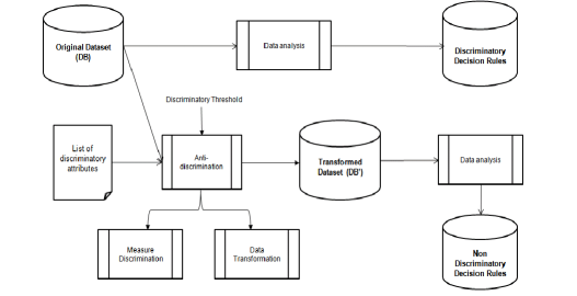
Figure 4.1: The process of extracting biased and unbiased decision rules

As mentioned before, background knowledge might be obtained from the original dataset itself because of the existence of PND attributes that are highly correlated with the PD ones in the original dataset. Let $BK$ be a database of background rules that is defined as

$$\mathcal{BK}=\{r_{b2}:D,B\rightarrow A|A\mbox{ discriminatory itemset and }supp(D,B\rightarrow A)\geq ms\}$$

In fact, $\mathcal{BK}$ is the set of classification rules $D,B\rightarrow A$ with a given minimum support $ms$ that shows the correlation between the PD itemset $A$ and the PND itemset $D$ with context $B$. Although rules of the form $r_{b1}:A,B\rightarrow D$ (in Theorem 1) are not included in $\mathcal{BK}$, $conf(r_{b1}:A,B\rightarrow D)$ could be obtained as $supp(r_{b2}:D,B\rightarrow A)/supp(B\rightarrow A)$.

4.4 Data Transformation for Direct Discrimination

The proposed solution to prevent direct discrimination is based on the fact that the dataset of decision rules would be free of direct discrimination if it only contained PD rules that are $\alpha$-protective or are instances of at least one non-redlining PND rule. Therefore, a suitable data transformation with minimum information loss should be applied in such a way that each $\alpha$-discriminatory rule either becomes $\alpha$-protective or an instance of a non-redlining PND rule. We call the first procedure direct rule protection and the second one rule generalization.

4.4.1 Direct Rule Protection (DRP)

In order to convert each $\alpha$-discriminatory rule into an $\alpha$-protective rule, based on the direct discriminatory measure $elift$ (i.e. Definition 3), we should enforce the following inequality for each $\alpha$-discriminatory rule $r^{\prime}:A,B\rightarrow C$ in $\mathcal{MR}$, where $A$ is a PD itemset:

$$elift(r^{\prime})<\alpha$$ (4.1)

By using the statement of the $elift$ Definition, Inequality (4.1) can be rewritten as

$$\frac{conf(r^{\prime}:A,B\rightarrow C)}{conf(B\rightarrow C)}<\alpha$$ (4.2)

Let us rewrite Inequality (4.2) in the following way

$$conf(r^{\prime}:A,B\rightarrow C)<\alpha\cdot conf(B\rightarrow C)$$ (4.3)

So, it is clear that Inequality (4.1) can be satisfied by decreasing the confidence of the $\alpha$-discriminatory rule $r^{\prime}:A,B\rightarrow C$ to a value less than the right-hand side of Inequality (4.3), without affecting the confidence of its base rule $B\rightarrow C$. A possible solution for decreasing

$$conf(r^{\prime}:A,B\rightarrow C)=\frac{supp(A,B,C)}{supp(A,B)}$$ (4.4)

is to perturb the discriminatory itemset from $\neg A$ to $A$ in the subset $\mathcal{D}_{c}$ of all records of the original dataset which completely support the rule $\neg A,B\rightarrow\neg C$ and have minimum impact on other rules; doing so increases the denominator of Expression (4.4) while keeping the numerator and $conf(B\rightarrow C$) unaltered.

There is also another way to provide direct rule protection. Let us rewrite Inequality (4.2) in the following different way

$$conf(B\rightarrow C)>\frac{conf(r^{\prime}:A,B\rightarrow C)}{\alpha}$$ (4.5)

It is clear that Inequality (4.1) can be satisfied by increasing the confidence of the base rule ($B\rightarrow C$) of the $\alpha$-discriminatory rule $r^{\prime}:A,B\rightarrow C$ to a value higher than the right-hand side of Inequality (4.5), without affecting the value of $conf(r^{\prime}:A,B\rightarrow C)$. A possible solution for increasing Expression

$$conf(B\rightarrow C)=\frac{supp(B,C)}{supp(B)}$$ (4.6)

is to perturb the class item from $\neg C$ to $C$ in the subset $\mathcal{DB}_{c}$ of all records of the original dataset which completely support the rule $\neg A,B\rightarrow\neg C$ and have minimum impact on other rules; doing so increases the numerator of Expression (4.6) while keeping the denominator and $conf(r^{\prime}:A,B\rightarrow C)$ unaltered.

Therefore, there are two methods that could be applied for direct rule protection. One method (Method 1) changes the PD itemset in some records (e.g. gender changed from male to female in the records with granted credits) and the other method (Method 2) changes the class item in some records (e.g. from grant credit to deny credit in the records with male gender). Thus, a suitable data transformation with minimum information loss should be applied in such a way that each $\alpha$-discriminatory rule $r$ becomes $\alpha$-protective by ensuring that $f(r)<\alpha$, where $f(r)$ could be one of the measures in Fig. 2.1. Then the general idea of our proposed method DRP for all these measures is the same. However, in the details (i.e. which records should be changed, how many records should be changed and how those records should be changed during data transformation), there could be some differences because of the different definition of these measures. For instance, in Table 4.1 we present all the possible data transformation methods for measures $elift$, $slift$ and $olift$ based on our proposed direct rule protection method.

Table 4.1: Data transformation methods (DTMs) for different measures

Measures	DTMs for DRP	Transformation requirement
$elift$	$\neg A,B\rightarrow\neg C\Rightarrow A,B\rightarrow\neg C$	$elift(A,B\rightarrow C)<\alpha$
	$\neg A,B\rightarrow\neg C\Rightarrow\neg A,B\rightarrow C$
$slift$	$A,B\rightarrow C\Rightarrow A,B\rightarrow\neg C$	$slift(A,B\rightarrow C)<\alpha$
	$\neg A,B\rightarrow\neg C\Rightarrow\neg A,B\rightarrow C$
$olift$	$\neg A,B\rightarrow\neg C\Rightarrow A,B\rightarrow\neg C$	$olift(A,B\rightarrow C)<\alpha$
	$\neg A,B\rightarrow\neg C\Rightarrow\neg A,B\rightarrow C$
	$A,B\rightarrow C\Rightarrow A,B\rightarrow\neg C$
	$A,B\rightarrow C\Rightarrow\neg A,B\rightarrow C$

As shown in Table 4.1, two possible data transformation methods for $elift$ are the same as two possible ones for $olift$ and one of them is the same as the possible ones for $slift$. Another point is that there is a method (the second one for each measure) that is the same for all three measures. Then we can conclude that for DRP not only the general idea is the same for different measures, but also in the details, there is a data transformation method applicable for all the measures.

4.4.2 Rule Generalization (RG)

Rule generalization is another data transformation method for direct discrimination prevention. It is based on the fact that if each $\alpha$-discriminatory rule $r^{\prime}:A,B\rightarrow C$ in the database of decision rules was an instance of at least one non-redlining (legitimate) PND rule $r:D,B\rightarrow C$, the dataset would be free of direct discrimination.

In rule generalization, we consider the relation between rules instead of discrimination measures. The following example illustrates this principle. Assume that a complainant claims discrimination against foreign workers among applicants for a job position. A classification rule $\{\mbox{Foreign worker=Yes},\mbox{City=NYC}\}\rightarrow\mbox{Hire=No}$ with high $elift$ supports the complainant’s claim. However, the decision maker could argue that this rule is an instance of a more general rule $\{\mbox{Experience=Low},\mbox{City=NYC}\}\rightarrow\mbox{Hire=No}$. In other words, foreign workers are rejected because of their low experience, not just because they are foreign. The general rule rejecting low-experienced applicants is a legitimate one, because experience can be considered a genuine/legitimate requirement for some jobs. To formalize this dependency among rules (i.e. $r^{\prime}$ is an instance of $r$), Pedreschi et al. in [70] say that a PD classification rule $r^{\prime}:A,B\rightarrow C$ is an instance of a PND rule $r:D,B\rightarrow C$ if rule $r$ holds with the same or higher confidence, namely $conf(r:D,B\rightarrow C)\geq conf(r^{\prime}:A,B\rightarrow C)$, and a case (record) satisfying discriminatory itemset $A$ in context $B$ satisfies legitimate itemset $D$ as well, namely $conf(A,B\rightarrow D)=1$. The two conditions can be relaxed as follows:

Definition 14.

Let $d\in[0,1]$. A classification rule $r^{\prime}:A,B\rightarrow C$ is a $d$-instance of $r:D,B\rightarrow C$ if both conditions below are true:

• Condition 1: $conf(r)\geq d\cdot conf(r^{\prime})$

• Condition 2: $conf(r^{\prime\prime}:A,B\rightarrow D)\geq d$.

Then, if $r^{\prime}$ is a $d$-instance of $r$ (where $d$ is 1 or a value near 1), $r^{\prime}$ is free of direct discrimination. Based on this concept, we propose a data transformation method (i.e. rule generalization) to transform each $\alpha$-discriminatory $r^{\prime}$ in $\mathcal{MR}$ into a $d$-instance of a legitimate rule. An important issue to perform rule generalization is to find a suitable PND rule ($r:D,B\rightarrow C$) or, equivalently, to find a suitable $D$ (e.g. Experience=Low). Although choosing non-redlining rules, as done in this chapter, is a way to obtain legitimate PND rules, sometimes it is not enough and a semantic hierarchy is needed to find the most suitable legitimate itemset.

At any rate, rule generalization can be attempted for $\alpha$-discriminatory rules $r^{\prime}$ for which there is at least one non-redlining PND rule $r$ satisfying at least one of the two conditions of Definition 14. If any of the two conditions does not hold, the original data should be transformed for it to hold. Let us assume that Condition (2) is satisfied but Condition (1) is not. Based on the definition of $d$-instance, to satisfy the first condition of Definition 14, we should enforce for each $\alpha$-discriminatory rule $r^{\prime}:A,B\rightarrow C$ in $\mathcal{MR}$ the following inequality, with respect to its PND rule $r:D,B\rightarrow C$:

$$conf(r:D,B\rightarrow C)\geq d\cdot conf(r^{\prime}:A,B\rightarrow C)$$ (4.7)

Let us rewrite Inequality (4.7) in the following way

$$conf(r^{\prime}:A,B\rightarrow C)\leq\frac{conf(r:D,B\rightarrow C)}{d}$$ (4.8)

So, it is clear that Inequality (4.7) can be satisfied by decreasing the confidence of the $\alpha$-discriminatory rule ($r^{\prime}:A,B\rightarrow C$) to values less than the right-hand side of Inequality (4.8), without affecting the confidence of rule $r:D,B\rightarrow C$ or the satisfaction of Condition (2) of Definition 14. The confidence of $r^{\prime}$ was previously specified in Expression (4.4). A possible solution to decrease this confidence is to perturb the class item from $C$ to $\neg C$ in the subset $\mathcal{D}_{c}$ of all records in the original dataset which completely support the rule $A,B,\neg D\rightarrow C$ and have minimum impact on other rules; doing so decreases the numerator of Expression (4.4) while keeping its denominator, $conf(r:D,B\rightarrow C)$ and also $conf(r":A,B\rightarrow D)$ (Condition (2) for rule generalization) unaltered.

Let us see what happens if if Condition (1) of Definition 14 is satisfied but Condition (2) is not. In this case, based on the definition of $d$-instance, to satisfy Condition (2) we should enforce the following inequality for each $\alpha$-discriminatory rule $r^{\prime}:A,B\rightarrow C$ in $\mathcal{MR}$ with respect to its PND rule $r:D,B\rightarrow C$:

$$conf(r":A,B\rightarrow D)\geq d$$ (4.9)

Inequality (4.9) must be satisfied by increasing the confidence of rule $r":A,B\rightarrow D$ to a value higher than $d$, without affecting the satisfaction of Condition (1). However, any effort at increasing the confidence of $r"$ impacts on the confidence of the $r$ or $r^{\prime}$ rules and might threaten the satisfaction of Condition (1) of Definition 14; indeed, in order to increase the confidence of $r"$ we must either decrease $supp(A,B)$ (which increases $conf(r^{\prime})$) or change $\neg D$ to $D$ for those records satisfying $A$ and $B$ (which decreases $conf(r)$). Hence, rule generalization can only be applied if Condition (2) is satisfied without any data transformation.

To recap, we see that rule generalization can be achieved provided that Condition (2) is satisfied, because Condition (1) can be reached by changing the class item in some records (e.g. from “Hire no” to “Hire yes” in the records of foreign and high-experienced people in NYC city).

4.4.3 Direct Rule Protection and Rule Generalization

Since rule generalization might not be applicable for all $\alpha$-discriminatory rules in $\mathcal{MR}$, rule generalization cannot be used alone for direct discrimination prevention and must be combined with direct rule protection. When applying both rule generalization and direct rule protection, $\alpha$-discriminatory rules are divided into two groups:

• $\alpha$-discriminatory rules $r^{\prime}$ for which there is at least one non-redlining PND rule $r$ satisfying Condition (2) of Definition 14. For these rules, rule generalization is performed unless direct rule protection requires less data transformation (in which case direct rule protection is used).

• $\alpha$-discriminatory rules such that there is no such PND rule. For these rules, direct rule protection is performed.

We propose Algorithm 1 to select the most appropriate discrimination prevention approach for each $\alpha$-discriminatory rule. First, for each $\alpha$-discriminatory rule in $\mathcal{MR}$ of type $r^{\prime}:A,B\rightarrow C$, a collection $D_{pn}$ of non-redlining PND rules of type $r:D,B\rightarrow C$ is found (Step 2). Then, the conditions of Definition 14 are checked for each rule in $D_{pn}$, for $d\geq 0.8$ (Steps 4-18). Three cases arise depending on whether Conditions (1) and (2) hold:

• Case 1: There is at least one rule $r\in D_{pn}$ such that both Conditions (1) and (2) of Definition 14 hold. In this case $r^{\prime}$ is a $d$-instance of $r$ for $d\geq 0.8$ and no transformation is required (Steps 19-20).

• Case 2: There is no rule in $D_{pn}$ satisfying both Conditions (1) and (2) of Definition 14, but there is at least one rule satisfying Condition (2). In this case (Step 23), the PND rule $r_{b}$ in $D_{pn}$ should be selected (Step 24) which requires the minimum data transformation to fulfill Condition (1). A smaller difference between the values of the two sides of Condition (1) for each $r$ in $D_{pn}$ indicates a smaller required data transformation. In this case the $\alpha$-discriminatory rule is transformed by rule generalization (Step 25).

• Case 3: No rule in $D_{pn}$ satisfies Condition (2) of Definition 14. In this case (Step 21), rule generalization is not possible and direct rule protection should be performed (Step 22).

Algorithm 1 Determining Discrimination Prevention Approaches

0: $\mathcal{DB}$, $\mathcal{MR}$, $\mathcal{FR}$, $d\geq 0.8$, $\alpha$

1: for each $r^{\prime}:A,B\rightarrow C\in\mathcal{MR}$ do

2:    $D_{pn}\leftarrow\mbox{Collection of non-redlining PND rules }r:D,B\rightarrow C$ from $FR$

3:    if $|D_{pn}|\neq 0$ then

4:       for each $r\in D_{pn}$ do

5:          // Assess conditions of $p$-instance

6:          Compute $conf(r")\mbox{, where }r":A,B\in D$

7:          if $conf(r)\geq d\cdot conf(r^{\prime})$ then

8:             $C1_{r}\leftarrow true$

9:          else

10:             $C1_{r}\leftarrow false$

11:             $dif1_{r}\leftarrow d\cdot conf(r^{\prime})-conf(r)$

12:          end if

13:          if $conf(r")\geq d$ then

14:             $C2_{r}\leftarrow true$

15:          else

16:             $C2_{r}\leftarrow false$

17:          end if

18:       end for

19:       if $\exists r\in D_{pn}\mbox{ s.t. }C1_{r}=true\wedge C2_{r}=true$ then

20:          $TR_{r^{\prime}}\leftarrow Nt$ // No transformation needed

21:       else if for all $r\in D_{pn}\mbox{, }C2_{r}=false$ then

22:          $TR_{r^{\prime}}\leftarrow DRP$ // Direct Rule Protection

23:       else if $\exists r\in D_{pn}\mbox{ s.t. }C2_{r}=true$ then

24:          $r_{b}\leftarrow r\in D_{pn}\mbox{ with minimum }dif1_{r}$

25:          $TR_{r^{\prime}}\leftarrow RG$ // Rule Generalization

26:       end if

27:    else

28:       // $|D_{pn}|=0$

29:       $TR_{r^{\prime}}\leftarrow DRP$ // Direct Rule Protection

30:    end if

31:    if $TR_{r^{\prime}}=RG$ then

32:       $dif_{r}^{\prime}\leftarrow conf(r^{\prime})-\alpha\cdot conf(B\rightarrow C$)

33:       if $dif_{r}^{\prime}<dif1_{r}$ then

34:          $TR_{r^{\prime}}\leftarrow DRP$

35:       end if

36:    end if

37: end for

37: $\mathcal{TR}$ containing all $r^{\prime}\in\mathcal{MR}$ and their respective $TR_{r^{\prime}}$ and $r_{b}$

For the $\alpha$-discriminatory rules to which rule generalization can be applied, it is possible that direct rule protection can be achieved with a smaller data transformation. For these rules the algorithm should select the approach with minimum transformation (Steps 31-36). The algorithm yields as output a database $\mathcal{TR}$ with all $r^{\prime}\in\mathcal{MR}$, their respective rule $r_{b}$ and their respective discrimination prevention approaches ($TR_{r^{\prime}}$).

4.5 Data Transformation for Indirect Discrimination

The proposed solution to prevent indirect discrimination is based on the fact that the dataset of decision rules would be free of indirect discrimination if it contained no redlining rules. To achieve this, a suitable data transformation with minimum information loss should be applied in such a way that redlining rules are converted to non-redlining rules. We call this procedure indirect rule protection.

4.5.1 Indirect Rule Protection (IRP)

In order to turn a redlining rule into an non-redlining rule, based on the indirect discriminatory measure (i.e. $elb$ in Theorem 1), we should enforce the following inequality for each redlining rule $r:D,B\rightarrow C$ in $\mathcal{RR}$:

$$elb(\gamma,\delta)<\alpha$$ (4.10)

By using the definitions stated when introducing $elb$ in Theorem 1, Inequality (4.10) can be rewritten as

$$\frac{\frac{conf(r_{b1})}{conf(r_{b2})}(conf(r_{b2})+conf(r:D,B\rightarrow C)-1)}{conf(B\rightarrow C)}<\alpha$$ (4.11)

Note that the discriminatory itemset (i.e. $A$) is not removed from the original database $\mathcal{D}$ and the rules $r_{b1}:A,B\rightarrow D$ and $r_{b2}:D,B\rightarrow A$ are obtained from $\mathcal{D}$, so that their confidences might change as a result of data transformation for indirect discrimination prevention. Let us rewrite Inequality (4.11) in the following way

$$conf(r_{b1}:A,B\rightarrow D)<\frac{\alpha\cdot conf(B\rightarrow C)\cdot conf(r_{b2})}{conf(r_{b2})+conf(r:D,B\rightarrow C)-1}$$ (4.12)

Clearly, in this case Inequality (4.10) can be satisfied by decreasing the confidence of rule $r_{b1}:A,B\rightarrow D$ to values less than the right-hand side of Inequality (4.12) without affecting either the confidence of the redlining rule or the confidence of the $B\rightarrow C$ and $r_{b2}$ rules. Since the values of both inequality sides are dependent, a transformation is required that decreases the left-hand side of the inequality without any impact on the right-hand side. A possible solution for decreasing

$$conf(A,B\rightarrow D)=\frac{supp(A,B,D)}{supp(A,B)}$$ (4.13)

in Inequality (4.12) to the target value is to perturb the discriminatory itemset from $\neg A$ to $A$ in the subset $\mathcal{D}_{c}$ of all records of the original dataset which completely support the rule $\neg A,B,\neg D\rightarrow\neg C$ and have minimum impact on other rules; this increases the denominator of Expression (4.13) while keeping the numerator and $conf(B\rightarrow C)$, $conf(r_{b2}:D,B\rightarrow A$), and $conf(r:D,B\rightarrow C$) unaltered.

There is another way to provide indirect rule protection. Let us rewrite Inequality (4.11) as Inequality (4.14), where the confidences of $r_{b1}$ and $r_{b2}$ rules are not constant.

$$conf(B\rightarrow C)>\frac{\frac{conf(r_{b1})}{conf(r_{b2})}(conf(r_{b2})+conf(r:D,B\rightarrow C)-1)}{\alpha}$$ (4.14)

Clearly, in this case Inequality (4.10) can be satisfied by increasing the confidence of the base rule ($B\rightarrow C$) of the redlining rule $r:D,B\rightarrow C$ to values greater than the right-hand side of Inequality (4.14) without affecting either the confidence of the redlining rule or the confidence of the $r_{b1}$ and $r_{b2}$ rules. A possible solution for increasing Expression (4.6) in Inequality (4.14) to the target value is to perturb the class item from $\neg C$ to $C$ in the subset $\mathcal{D}_{c}$ of all records of the original dataset which completely support the rule $\neg A,B,\neg D\rightarrow\neg C$ and have minimum impact on other rules; this increases the numerator of Expression (4.6) while keeping the denominator and $conf(r_{b1}:A,B\rightarrow D$), $conf(r_{b2}:D,B\rightarrow A$), and $conf(r:D,B\rightarrow C$) unaltered.

Hence, like in direct rule protection, there are also two methods that could be applied for indirect rule protection. One method (Method 1) changes the discriminatory itemset in some records (e.g. from non-foreign worker to foreign worker in the records of hired people in NYC city with Zip$\neq$10451) and the other method (Method 2) changes the class item in some records (e.g. from “Hire yes” to “Hire no” in the records of non-foreign worker of people in NYC city with Zip$\neq$10451).

4.6 Data Transformation for Both Direct and Indirect Discrimination

We deal here with the key problem of transforming data with minimum information loss to prevent at the same time both direct and indirect discrimination. We will give a pre-processing solution to simultaneous direct and indirect discrimination prevention. First, we explain when direct and indirect discrimination could simultaneously occur. This depends on whether the original dataset ($\mathcal{D}$) contains discriminatory itemsets or not. Two cases arise:

• PD itemsets (i.e. $A$) did not exist in the original database $\mathcal{D}$ or have previously been removed from it due to privacy constraints or for preventing discrimination. However, if background knowledge from publicly available data (e.g. census data) is available, indirect discrimination remains possible. In fact, in this case, only PND rules are extracted from $\mathcal{D}$ so only indirect discrimination could happen.

• At least one PD itemset (i.e. $A$) is not removed from the original database ($\mathcal{D}$). So it is clear that PD rules could be extracted from $\mathcal{D}$ and direct discrimination could happen. However, in addition to direct discrimination, indirect discrimination might occur because of background knowledge obtained from $\mathcal{D}$ itself due to the existence of PND items that are highly correlated with the sensitive (discriminatory) ones. Hence, in this case both direct and indirect discrimination could happen.

To provide both direct rule protection (DRP) and indirect rule protection (IRP) at the same time, an important point is the relation between the data transformation methods. Any data transformation to eliminate direct $\alpha$-discriminatory rules should not produce new redlining rules or prevent the existing ones from being removed. Also

Table 4.2: Direct and indirect rule protection methods

	Method 1	Method 2
Direct Rule Protection	$\neg A,B\rightarrow\neg C\Rightarrow A,B\rightarrow\neg C$	$\neg A,B\rightarrow\neg C\Rightarrow\neg A,B\rightarrow C$
Indirect Rule Protection	$\neg A,B,\neg D\rightarrow\neg C\Rightarrow A,B,\neg D\rightarrow\neg C$	$\neg A,B,\neg D\rightarrow\neg C\Rightarrow\neg A,B,\neg D\rightarrow C$

any data transformation to eliminate redlining rules should not produce new direct $\alpha$-discriminatory rules or prevent the existing ones from being removed.

For subsequent use in this section, we summarize in Table 4.2 the methods for DRP and IRP described in Sections 4.4.1 and 4.5.1 above. We can see in Table 4.2 that DRP and IRP operate the same kind of data transformation: in both cases Method 1 changes the PD itemset, whereas Method 2 changes the class item. Therefore, in principle any data transformation for DRP (resp. IRP) not only does not need to have a negative impact on IRP (resp. DRP), but both kinds of protection could even be beneficial to each other.

However, there is a difference between DRP and IRP: the set of records chosen for transformation. As shown in Table 4.2, in IRP the chosen records should not satisfy the $D$ itemset (chosen records are those with $\neg A,B,\neg D\rightarrow\neg C$), whereas DRP does not care about $D$ at all (chosen records are those with $\neg A,B\rightarrow\neg C$). The following interactions between direct and indirect rule protection become apparent.

Lemma 1.

Method 1 for DRP cannot be used if simultaneous DRP and IRP are desired.

Proof: Method 1 for DRP might undo the protection provided by Method 1 for IRP, as we next justify. Method 1 for DRP decreases $conf(A,B\rightarrow C)$ until the direct rule protection requirement (Inequality (4.3)) is met and Method 1 for IRP needs to decrease $conf(A,B\rightarrow D)$ until the indirect rule protection requirement is met (Inequality (4.12)). Assume that decreasing $conf(A,B\rightarrow C)$ to meet the direct rule protection requirement is achieved by changing $y$ (how $y$ is obtained will be discussed in Section 4.8) number of records with $\neg A,B,\neg C$ to records with $A,B,\neg C$ (as done by Method 1 for DRP). This actually could increase $conf(A,B\rightarrow D)$ if $z$ among the changed records, with $z\leq y$, turn out to satisfy $D$. This increase can undo the protection provided by Method 1 for IRP (i.e. $conf(A,B\rightarrow D)<IRP_{req1}$, where $IRP_{req1}=\frac{\alpha\cdot conf(B\rightarrow C)\cdot conf(r_{b2})}{conf(r_{b2})+conf(r:D,B\rightarrow C)-1}$) if the new value $conf(A,B\rightarrow D)=\frac{supp(A,B,D)+z}{supp(A,B)+y}$ is greater than or equal to $IRP_{req1}$, which happens if $z\geq IRP_{req1}\cdot(supp(A,B)+Y)-supp(A,B,D)$. $\Box$

Lemma 2.

Method 2 for IRP is beneficial for Method 2 for DRP. On the other hand, Method 2 for DRP is at worst neutral for Method 2 for IRP.

Proof: Method 2 for DRP and Method 2 for IRP are both aimed at increasing $conf(B\rightarrow C)$. In fact, Method 2 for IRP changes a subset of the records changed by Method 2 for DRP. This proves that Method 2 for IRP is beneficial for Method 2 for DRP. On the other hand, let us check that, in the worst case, Method 2 for DRP is neutral for Method 2 for IRP: such a worst case is the one in which all changed records satisfy $D$, which could result in increasing both sides of Inequality (4.14) by an equal amount (due to increasing $conf(B\rightarrow C)$ and $conf(D,B\rightarrow C)$); even in this case, there is no change in whatever protection is achieved by Method 2 for IRP. $\Box$

Thus, we conclude that Method 2 for DRP and Method 2 for IRP are the only methods among those described that can be applied to achieve simultaneous direct and indirect discrimination prevention. In addition, in the cases where either only direct or only indirect discrimination exist, there is no interference between the described methods: Method 1 for DRP, Method 2 for DRP and Rule Generalization can be used to prevent direct discrimination; Method 1 for IRP and Method 2 for IRP can be used to prevent indirect discrimination. In what follows, we propose algorithms based on the described methods that cover direct and/or indirect discrimination prevention.

4.7 The Algorithms

We describe in this section our algorithms based on the direct and indirect discrimination prevention methods proposed in Sections 4.4,  4.5 and 4.6. There are some assumptions common to all algorithms in this section. First, we assume the class attribute in the original dataset $\mathcal{D}$ to be binary (e.g. denying or granting credit). Second, we consider classification rules with negative decision (e.g. denying credit) to be in $\mathcal{FR}$. Third, we assume the PD itemsets (i.e. $A$) and the PND itemsets (i.e. $D$) to be binary or non-binary categorical.

4.7.1 Direct Discrimination Prevention Algorithms

We start with direct rule protection. Algorithm 2 details Method 1 for DRP. For each direct $\alpha$-discriminatory rule $r^{\prime}$ in $\mathcal{MR}$ (Step 3), after finding the subset $\mathcal{D}_{c}$ (Step 5), records in $\mathcal{D}_{c}$ should be changed until the direct rule protection requirement (Step 10) is met for each respective rule (Steps 10-14).

Among the records of $\mathcal{D}_{c}$, one should change those with lowest impact on the other ($\alpha$-protective or non-redlining) rules. Hence, for each record $db_{c}\in\mathcal{D}_{c}$, the number of rules whose premise is supported by $db_{c}$ is taken as the impact of $db_{c}$ (Step 7), that is $impact(db_{c})$; the rationale is that changing $db_{c}$ impacts on the confidence of those rules. Then the records $db_{c}$ with minimum $impact(db_{c})$ are selected for change (Step 9), with the aim of scoring well in terms of the utility measures proposed in the next section. We call this procedure (Steps 6-9) impact minimization and we re-use it in the pseudocodes of the rest of algorithms specified in this chapter.

Algorithm 2 Direct Rule Protection (Method 1)

1:  Inputs: $\mathcal{D}$, $\mathcal{FR}$, $\mathcal{MR}$, $\alpha$, $DI_{b}$

2:  Output: $\mathcal{D^{\prime}}$ (transformed dataset)

3:  for each $r^{\prime}:A,B\rightarrow C\in\mathcal{MR}$ do

4:     $\mathcal{FR}\leftarrow\mathcal{FR}-\{r^{\prime}\}$

5:     $\mathcal{D}_{c}\leftarrow\mbox{All records completely supporting }\neg A,B\rightarrow\neg C$

6:     for each $db_{c}\in\mathcal{D}_{c}$ do

7:        Compute $impact(db_{c})=|\{r_{a}\in\mathcal{FR}|db_{c}$ supports the premise of $r_{a}\}|$

8:     end for

9:     Sort $\mathcal{D}_{c}$ by ascending impact

10:     while $conf(r^{\prime})\geq\alpha\cdot conf(B\rightarrow C)$ do

11:        Select first record in $\mathcal{D}_{c}$

12:        Modify PD itemset of $db_{c}$ from $\neg A$ to $A$ in $\mathcal{D}$

13:        Recompute $conf(r^{\prime})$

14:     end while

15:  end for

16:  Output: $\mathcal{D^{\prime}}=\mathcal{D}$

Algorithm 3 details Method 2 for DRP. The parts of Algorithm 3 to find subset $\mathcal{D}_{c}$ and perform impact minimization (Step 4) are the same as in Algorithm 2. However, the transformation requirement that should be met for each $\alpha$-discriminatory rule in $\mathcal{MR}$ (Step 5) and the kind of data transformation are different (Steps 5-9).

Algorithm 3 Direct Rule Protection (Method 2)

1:  Inputs: $\mathcal{D}$, $\mathcal{FR}$, $\mathcal{MR}$, $\alpha$, $DI_{b}$

2:  Output: $\mathcal{D^{\prime}}$ (transformed dataset)

3:  for each $r^{\prime}:A,B\rightarrow C\in\mathcal{MR}$ do

4:     Steps 4-9 Algorithm 2

5:     while $conf(B\rightarrow C)\leq\frac{conf(r^{\prime})}{\alpha}$ do

6:        Select first record in $\mathcal{D}_{c}$

7:        Modify the class item of $db_{c}$ from $\neg C$ to $C$ in $\mathcal{D}$

8:        Recompute $conf(B\rightarrow C)$

9:     end while

10:  end for

11:  Output: $\mathcal{D^{\prime}}=\mathcal{D}$

As mentioned in Section 4.4.3, rule generalization cannot be applied alone for solving direct discrimination prevention, but it can be used in combination with Method 1 or Method 2 for DRP. In this case, after specifying the discrimination prevention method (i.e. direct rule protection or rule generalization) to be applied for each $\alpha$-discriminatory rule based on the algorithm in Section 4.4.3, Algorithm 4 should be run to combine rule generalization and one of the two direct rule protection methods.

Algorithm 4 Direct Rule Protection and Rule Generalization

1:  Inputs: $\mathcal{D}$, $\mathcal{FR}$, $\mathcal{TR}$, $p\geq 0.8$, $\alpha$, $DI_{b}$

2:  Output: $\mathcal{D^{\prime}}$ (transformed dataset)

3:  for each $r^{\prime}:A,B\rightarrow C\in\mathcal{TR}$ do

4:     $\mathcal{FR}\leftarrow\mathcal{FR}-\{r^{\prime}\}$

5:     if $TR_{r^{\prime}}$ = RG then

6:        // Rule Generalization

7:        $\mathcal{D}_{c}\leftarrow\mbox{All records completely supporting }A,B,\neg D\rightarrow C$

8:        Steps 6-9 Algorithm 2

9:        while $conf(r^{\prime})>\frac{conf(r_{b}:D,B\rightarrow C)}{p}$ do

10:           Select first record in $\mathcal{D}_{c}$

11:           Modify class item of $db_{c}$ from $C$ to $\neg C$ in $\mathcal{D}$

12:           Recompute $conf(r^{\prime})$

13:        end while

14:     end if

15:     if $TR_{r^{\prime}}$ = DRP then

16:        // Direct Rule Protection

17:        Steps 5-14 Algorithm 2 or Steps 4-9 Algorithm 3

18:     end if

19:  end for

20:  Output: $\mathcal{D^{\prime}}=\mathcal{D}$

Algorithm 4 takes as input $\mathcal{TR}$, which is the output of the algorithm in Section 4.4.3, containing all $r^{\prime}\in\mathcal{MR}$ and their respective $TR_{r^{\prime}}$ and $r_{b}$. For each $\alpha$-discriminatory rule $r^{\prime}$ in $\mathcal{TR}$, if $TR_{r^{\prime}}$ shows that rule generalization should be performed (Step 5), after determining the records that should be changed for impact minimization (Steps 7-8), these records should be changed until the rule generalization requirement is met (Steps 9-13). Also, if $TR_{r^{\prime}}$ shows that direct rule protection should be performed (Step 15), based on either Method 1 or Method 2, the relevant sections of Algorithm 2 or  3 are called, respectively (Step 17).

4.7.2 Indirect Discrimination Prevention Algorithms

A detailed algorithm implementing Method 2 for IRP is provided in [35], from which an algorithm implementing Method 1 for IRP can be easily derived. Due to similarity with the previous algorithms, we do not recall those two algorithms for IRP here.

4.7.3 Direct and Indirect Discrimination Prevention Algorithms

Algorithm 5 details our proposed data transformation method for simultaneous direct and indirect discrimination prevention. The algorithm starts with redlining rules. From each redlining rule ($r:X\rightarrow C$), more than one indirect $\alpha$-discriminatory rule ($r^{\prime}:A,B\rightarrow C$) might be generated because of two reasons: 1) existence of different ways to group the items in $X$ into a context itemset $B$ and a PND itemset $D$ correlated to some PD itemset $A$; and 2) existence of more than one item in $DI_{b}$. Hence, as shown in Algorithm 5 (Step 5), given a redlining rule $r$, proper data transformation should be conducted for all indirect $\alpha$-discriminatory rules $r^{\prime}:(A\subseteq DI_{b}),(B\subseteq X)\rightarrow C$ ensuing from $r$.

Algorithm 5 Direct and Indirect Discrimination Prevention

1: Inputs: $\mathcal{D}$, $\mathcal{FR}$, $\mathcal{RR}$, $\mathcal{MR}$, $\alpha$, $DI_{b}$

2: Output: $\mathcal{D^{\prime}}$ (transformed dataset)

3: for each $r:X\rightarrow C\in\mathcal{RR}$, where $D,B\subseteq X$ do

4:    $\gamma=conf(r)$

5:    for each $r^{\prime}:(A\subseteq DI_{b}),(B\subseteq X)\rightarrow C\in\mathcal{RR}$ do

6:       $\beta_{2}=conf(r_{b2}:X\rightarrow A)$

7:       $\Delta_{1}=supp(r_{b2}:X\rightarrow A)$

8:       $\delta=conf(B\rightarrow C)$

9:       $\Delta_{2}=supp(B\rightarrow A)$

10:       $\beta_{1}=\frac{\Delta_{1}}{\Delta_{2}}$              //$conf(r_{b1}:A,B\rightarrow D)$

11:       Find $\mathcal{D}_{c}$: all records in $\mathcal{D}$ that completely support $\neg A,B,\neg D\rightarrow\neg C$

12:       Steps 6-9 Algorithm 2

13:       if $r^{\prime}\in\mathcal{MR}$ then

14:          while $(\delta\leq\frac{\beta_{1}(\beta_{2}+\gamma-1)}{\beta_{2}\cdot\alpha})$ and $(\delta\leq\frac{conf(r^{\prime})}{\alpha})$ do

15:             Select first record $db_{c}$ in $\mathcal{D}_{c}$

16:             Modify the class item of $db_{c}$ from $\neg C$ to $C$ in $\mathcal{D}$

17:             Recompute $\delta=conf(B\rightarrow C)$

18:          end while

19:       else

20:          while $\delta\leq\frac{\beta_{1}(\beta_{2}+\gamma-1)}{\beta_{2}\cdot\alpha}$ do

21:             Steps 15-17 Algorithm 5

22:          end while

23:       end if

24:    end for

25: end for

26: for each $r^{\prime}:(A,B\rightarrow C)\in\mathcal{MR}\setminus\mathcal{RR}$ do

27:    $\delta=conf(B\rightarrow C)$

28:    Find $\mathcal{D}_{c}$: all records in $\mathcal{D}$ that completely support $\neg A,B\rightarrow\neg C$

29:    Step 12

30:    while $(\delta\leq\frac{conf(r^{\prime})}{\alpha})$ do

31:       Steps 15-17 Algorithm 5

32:    end while

33: end for

34: Output: $\mathcal{D^{\prime}}=\mathcal{D}$

If some rules can be extracted from $\mathcal{D}$ as both direct and indirect $\alpha$-discriminatory rules, it means that there is overlap between $\mathcal{MR}$ and $\mathcal{RR}$; in such case, data transformation is performed until both the direct and the indirect rule protection requirements are satisfied (Steps 13-18). This is possible because, as we showed in Section 4.6, the same data transformation method (Method 2 consisting of changing the class item) can provide both DRP and IRP. However, if there is no overlap between $\mathcal{MR}$ and $\mathcal{RR}$, the data transformation is performed according to Method 2 for IRP, until the indirect discrimination prevention requirement is satisfied (Steps 19-23) for each indirect $\alpha$-discriminatory rule ensuing from each redlining rule in $\mathcal{RR}$; this can be done without any negative impact on direct discrimination prevention, as justified in Section 4.6. Then, for each direct $\alpha$-discriminatory rule $r^{\prime}\in\mathcal{MR}\setminus\mathcal{RR}$ (that is only directly extracted from $\mathcal{D}$), data transformation for satisfying the direct discrimination prevention requirement is performed (Steps 26-33), based on Method 2 for DRP; this can be done without any negative impact on indirect discrimination prevention, as justified in Section 4.6. Performing rule protection or generalization for each rule in $\mathcal{MR}$ by each of Algorithms 2- 5 has no adverse effect on protection for other rules (i.e. rule protection at Step $i+x$ to make $r^{\prime}$ protective cannot turn into discriminatory a rule $r$ made protective at Step $i$) because of the two following reasons: the kind of data transformation for each rule is the same (change the PD itemset or the class item of records) and there are no two $\alpha$-discriminatory rules $r$ and $r^{\prime}$ in $\mathcal{MR}$ such that $r=r^{\prime}$.

4.8 Computational Cost

The computational cost of Algorithm 2 can be broken down as follows:

• Let $m$ be the number of records in $\mathcal{D}$. The cost of finding subset $\mathcal{D}_{c}$ (Step 5) is $O(m)$.

• Let $k$ be the number of rules in $\mathcal{FR}$ and $h$ the number of records in subset $\mathcal{D}_{c}$. The cost of computing $impact(db_{c})$ for all records in $\mathcal{D}_{c}$ (Steps 6-8) is $O(hk)$.

• The cost of sorting $\mathcal{D}_{c}$ by ascending impact (Step 9) is $O(h\log h)$. Then, the cost of the impact minimization procedure (Steps 6-9) in all algorithms is $O(hk+h\log h)$.

• During each iteration of the inner loop (Step 10), the number of records supporting the premise of rule $r^{\prime}:A,B\rightarrow C$ is increased by one. After $i$ iterations, the confidence of $r^{\prime}:A,B\rightarrow C$ will be $conf(r^{\prime}:A,B\rightarrow C)^{(i)}=\frac{N_{ABC}}{N_{AB}+i}$, where $N_{ABC}$ is the number of records supporting rule $r^{\prime}$ and $N_{AB}$ is the number of records supporting the premise of rule $r^{\prime}$. If we let $DRP_{req1}=\alpha\cdot conf(B\rightarrow C)$, the inner loop (Step 10) is iterated until $conf(r^{\prime}:A,B\rightarrow C)^{(i)}<DRP_{req1}$ or equivalently $\frac{N_{ABC}}{N_{AB}+i}<DRP_{req1}$. This inequality can be rewritten as $i>(\frac{N_{ABC}}{DRP_{req1}}-N_{BC})$. From this last inequality we can derive that $i=\lceil\frac{N_{ABC}}{DRP_{req1}}-N_{BC}\rceil$. Hence, iterations in the inner loop (Step 10) will stop as soon as the first integer value greater than (or equal) $\frac{N_{ABC}}{DRP_{req1}}-N_{BC}$ is reached. Then, the cost spent on the inner loop to satisfy the direct rule protection requirement (Steps 10-14) will be $O(m*\lceil\frac{N_{ABC}}{DRP_{req1}}-N_{BC}\rceil)$.

Therefore, assuming $n$ is the number of $\alpha$-discriminatory rules in $\mathcal{MR}$ (Step 3), the total computational time of Algorithm 2 is bounded by $O(n*\{m+hk+h\log h+im\})$, where $i=\lceil\frac{N_{ABC}}{DRP_{req1}}-N_{BC}\rceil$.

The impact minimization procedure substantially increases the complexity. Without computing the impact, the time complexity of Algorithm 2 decreases to $O(n*\{m+im\})$. In addition, it is clear that the execution time of Algorithm 2 increases linearly with the number $m$ of original data records as well as the number $k$ of frequent classification rules and the number $n$ of $\alpha$-discriminatory rules.

The computational cost of the other algorithms can be computed similarly, with some small differences. In summary, the total computational time of Algorithm 3 is also bounded by $O(n*\{m+hk+h\log h+im\})$, where $i=\lceil({N_{B}}*DRP_{req2})-N_{BC}\rceil$, $N_{BC}$ is the number of records supporting rule $B\rightarrow C$, $N_{B}$ is the number of records supporting itemset $B$ and $DRP_{req2}=\frac{conf(r^{\prime})}{\alpha}$. The computational cost of Algorithm 4 is the same as the last ones with the difference that $i=\lceil{N_{ABC}-(RG_{req}*N_{AB})}\rceil$, where $RG_{req}=\frac{conf(r_{b})}{d}$, or $i=\lceil({N_{B}}*DRP_{req2})-N_{BC}\rceil$, depending on whether rule generalization or direct rule protection is performed.

Finally, assuming $f$ is the number of indirect $\alpha$-discriminatory rules in $\mathcal{RR}$ and $n$ is the number of direct $\alpha$-discriminatory rules in $\mathcal{MR}$ that no longer exist in $\mathcal{RR}$, the total computational time of Algorithm 5 is bounded by $O((f+n)*\{m+hk+h\log h+im\})$, where $i=\lceil({N_{B}}*max_{req})-N_{BC}\rceil$ and $max_{req}=\max(\frac{\beta_{1}(\beta_{2}+\gamma-1)}{\beta_{2}\cdot\alpha},\frac{conf(r^{\prime})}{\alpha})$.

4.9 Experiments

This section presents the experimental evaluation of the proposed direct and/or indirect discrimination prevention approaches and algorithms. To obtain $\mathcal{FR}$ and $\mathcal{BK}$ we used the Apriori algorithm [2], which is a common algorithm to extract frequent rules. All algorithms and utility measures were implemented using the C# programming language. The tests were performed on an 2.27 GHz Intel® Core™i3 machine, equipped with 4 GB of RAM, and running under Windows 7 Professional.

First, we describe the datasets used in our experiments. Then, we introduce the new utility measures we propose to evaluate direct and indirect discrimination prevention methods in terms of their success at discrimination removal and impact on data quality. Finally, we present the evaluation results of the different methods and also the comparison between them.

4.9.1 Datasets

Adult dataset: We used the Adult dataset from  [25], also known as Census Income, in our experiments. This dataset consists of 48,842 records, split into a “train” part with 32,561 records and a “test” part with 16,281 records. The dataset has 14 attributes (without class attribute). We used the “train” part in our experiments. The prediction task associated to the Adult dataset is to determine whether a person makes more than 50K$ a year based on census and demographic information about people. The dataset contains both categorical and numerical attributes.

For our experiments with the Adult dataset, we set $DI_{b}$={Sex=Female, Age=Young}. Although the Age attribute in the Adult dataset is numerical, we converted it to categorical by partitioning its domain into two fixed intervals: Age $\leq$ 30 was renamed as Young and Age $>$ 30 was renamed as old.

German Credit dataset: We also used the German Credit dataset from [25]. This dataset consists of 1,000 records and 20 attributes (without class attribute) of bank account holders. This is a well-known real-life dataset, containing both numerical and categorical attributes. It has been frequently used in the anti-discrimination literature  [68, 43]. The class attribute in the German Credit dataset takes values representing good or bad classification of the bank account holders. For our experiments with this dataset, we set $DI_{b}$= {Foreign worker=Yes, Personal Status=Female and not Single, Age=Old} (cut-off for Age=Old: 50 years old).

4.9.2 Utility Measures

Our proposed techniques should be evaluated based on two aspects. On the one hand, we need to measure the success of the method in removing all evidence of direct and/or indirect discrimination from the original dataset; on the other hand, we need to measure the impact of the method in terms of information loss (i.e. data quality loss). To measure discrimination removal, four metrics were used:

• Direct Discrimination Prevention Degree (DDPD). This measure quantifies the percentage of $\alpha$-discriminatory rules that are no longer $\alpha$-discriminatory in the transformed dataset. We define DDPD as

  $$DDPD=\frac{|\mathcal{MR}|-|\mathcal{MR}^{\prime}|}{|\mathcal{MR}|}$$

  where $\mathcal{MR}$ is the database of $\alpha$-discriminatory rules extracted from $\mathcal{D}$ and $\mathcal{MR}^{\prime}$ is the database of $\alpha$-discriminatory rules extracted from the transformed dataset $\mathcal{D}^{\prime}$. Note that $|\cdot|$ is the cardinality operator.

• Direct Discrimination Protection Preservation (DDPP). This measure quantifies the percentage of the $\alpha$-protective rules in the original dataset that remain $\alpha$-protective in the transformed dataset. It is defined as

  $$DDPP=\frac{|\mathcal{PR}\bigcap\mathcal{PR}^{\prime}|}{|\mathcal{PR}|}$$

  where $\mathcal{PR}$ is the database of $\alpha$-protective rules extracted from the original dataset $\mathcal{D}$ and $\mathcal{PR}^{\prime}$ is the database of $\alpha$-protective rules extracted from the transformed dataset $\mathcal{D}^{\prime}$.

• Indirect Discrimination Prevention Degree (IDPD) This measure quantifies the percentage of redlining rules that are no longer redlining in the transformed dataset. It is defined like DDPD but substituting $\mathcal{MR}$ and $\mathcal{MR}^{\prime}$ with the database of redlining rules extracted from $\mathcal{D}$ and $\mathcal{D}^{\prime}$, respectively.

• Indirect Discrimination Protection Preservation (IDPP) This measure quantifies the percentage of non-redlining rules in the original dataset that remain non-redlining in the transformed dataset. It is defined like DDPP but substituting $\mathcal{PR}$ and $\mathcal{PR}^{\prime}$ with the database of non-redlining extracted from $\mathcal{D}$ and $\mathcal{D}^{\prime}$, respectively.

Since the above measures are used to evaluate the success of the proposed method in direct and indirect discrimination prevention, ideally their value should be 100%. To measure data quality, we use two metrics proposed in the literature as information loss measures in the context of rule hiding for privacy-preserving data mining (PPDM) [88].

• Misses Cost (MC). This measure quantifies the percentage of rules among those extractable from the original dataset that cannot be extracted from the transformed dataset (side-effect of the transformation process).

• Ghost Cost (GC). This measure quantifies the percentage of the rules among those extractable from the transformed dataset that were not extractable from the original dataset (side-effect of the transformation process).

MC and GC should ideally be 0%. However, MC and GC may not be 0% as a side-effect of the transformation process.

4.9.3 Empirical Evaluation

We implemented the algorithms for all proposed methods for direct and/or indirect discrimination prevention, and we evaluated them in terms of the proposed utility measures. We report the performance results in this section.

Tables 4.3 and  4.4 show the utility scores obtained by our methods on the Adult dataset and the German Credit dataset, respectively. Within each table, the first row relates to the simple approach of deleting discriminatory attributes, the next four rows relate to direct discrimination prevention methods, the next two ones relate to indirect discrimination prevention methods and the last one relates to the combination of direct and indirect discrimination.

Table 4.3: Adult dataset: Utility measures for minimum support 2% and confidence 10% for all the methods. Value “n.a.” denotes that the respective measure is not applicable.

Methods	$\alpha$	$p$	No.	No. Indirect	No. Direct	Disc. Removal				Data Quality
			Redlining	$\alpha$-Disc.	$\alpha$-Disc.	Direct		Indirect
			Rules	Rules	Rules	DDPD	DDPP	IDPD	IDPP	MC	GC
Removing. Disc. Attributes	n.a.	n.a	n.a.	n.a	n.a.	n.a.	n.a.	n.a.	n.a.	66.08	0
DRP (Method 1)	1.2	n.a	n.a.	n.a	274	100	100	n.a.	n.a.	4.16	4.13
DRP (Method 2)	1.2	n.a.	n.a.	n.a.	274	100	100	n.a.	n.a.	0	0
DRP (Method 1) + RG	1.2	0.9	n.a.	n.a.	274	100	100	n.a.	n.a.	4.1	4.1
DRP (Method 2) + RG	1.2	0.9	n.a.	n.a.	274	91.58	100	n.a.	n.a.	0	0
IRP (Method 1)	1.1	n.a.	21	30	n.a.	n.a.	n.a.	100	100	0.54	0.38
IRP (Method 2)	1.1	n.a.	21	30	n.a.	n.a.	n.a.	100	100	0	0
DRP(Method 2) + IRP(Method 2)	1.1	n.a.	21	30	280	100	100	100	100	0	0
No of Freq. Class. Rules: 5,092						No. of Back. Know. Rules: 2089

Table 4.4: German Credit dataset: Utility measures for minimum support 5% and confidence 10% for all methods. Value “n.a.” denotes that the respective measure is not applicable.

Methods	$\alpha$	$p$	No.	No. Indirect	No. Direct	Discrimination Removal				Data Quality
			Redlining	$\alpha$-Disc.	$\alpha$-Disc.	Direct		Indirect
			Rules	Rules	Rules	DDPD	DDPP	IDPD	IDPP	MC	GC
Removing. Disc. Attributes	n.a.	n.a	n.a.	n.a	n.a.	n.a.	n.a.	n.a.	n.a.	64.35	0
DRP (Method 1)	1.2	n.a	n.a.	n.a	991	100	100	n.a.	n.a.	15.44	13.52
DRP (Method 2)	1.2	n.a.	n.a.	n.a.	991	100	100	n.a.	n.a.	0	4.06
DRP (Method 1) + RG	1.2	0.9	n.a.	n.a.	991	100	100	n.a.	n.a.	13.34	12.01
DRP (Method 2) + RG	1.2	0.9	n.a.	n.a.	991	100	100	n.a.	n.a.	0.01	4.06
IRP (Method 1)	1	n.a.	37	42	n.a.	n.a.	n.a.	100	100	1.62	1.47
IRP (Method 2)	1	n.a.	37	42	n.a.	n.a.	n.a.	100	100	0	0.96
DRP(Method 2) + IRP(Method 2)	1	n.a.	37	42	499	99.97	100	100	100	0	2.07
No of Freq. Class. Rules: 32,340						No. of Back. Know. Rules: 22,763

Table 4.3 shows the results for minimum support 2% and minimum confidence 10%. Table 4.4 shows the results for minimum support 5% and minimum confidence 10%. In Tables 4.3 and  4.4, the results of direct discrimination prevention methods are reported for discriminatory threshold $\alpha=1.2$ and, in the cases where direct rule protection is applied in combination with rule generalization, we used $d=0.9$, and $DI_{b}$={Sex=Female, Age=Young} in the Adult dataset, and $DI_{b}$= {Foreign worker=Yes, Personal Status=Female and not Single, Age=Old} in the German Credit dataset. In addition, in Table 4.3, the results of the indirect discrimination prevention methods and both direct and indirect discrimination prevention are reported for discriminatory threshold $\alpha=1.1$ and $DI_{b}$={Sex=Female, Age=Young}; in Table 4.4, these results are reported for $\alpha=1$ and $DI_{b}$= {Foreign worker=Yes}).

We selected the discriminatory threshold values and $DI_{b}$ for each dataset in such a way that the number of redlining rules and $\alpha$-discriminatory rules extracted from $\mathcal{D}$ could be suitable to test all our methods. In addition to the scores of utility measures, the number of redlining rules, the number of indirect $\alpha$-discriminatory rules and the number of direct $\alpha$-discriminatory rules are also reported in Tables 4.3 and  4.4. These tables also show the number of frequent classification rules found, as well as the number of background knowledge rules related to this experiment.

As shown in Tables 4.3 and  4.4, we get very good results for all methods in terms of discrimination removal: DDPD, DDPP, IDPD, IDPP are near 100% for both datasets. In terms of data quality, the best results for direct discrimination prevention are obtained with Method 2 for DRP or Method 2 for DRP combined with Rule Generalization. The best results for indirect discrimination prevention are obtained with Method 2 for IRP. This shows that lower information loss is obtained with the methods changing the class item (i.e. Method 2) than with those changing the discriminatory itemset (i.e. Method 1). As mentioned above, in direct discrimination prevention, rule generalization cannot be applied alone and must be applied in combination with direct rule protection; however, direct rule protection can be applied alone. The results in the last row of the above tables (i.e. Method 2 for DRP + Method 2 for IRP) based on Algorithm 5 for the case of simultaneous direct and indirect discrimination demonstrate that the proposed solution achieves a high degree of simultaneous direct and indirect discrimination removal with very little information loss.

For all methods, Tables 4.3 and 4.4 show that we obtained lower information loss in terms of MC and GC in the Adult dataset than in the German Credit dataset. In terms of discrimination removal, results on both datasets were almost the same. In addition, the highest value of information loss is obtained by the simple approach of removing discriminatory attributes (first row of each table): as it could be expected, entirely suppressing the PD attributes is much more information-damaging than modifying the values of these attributes in a few records.

Figure 4.2: Information loss (left) and discrimination removal degree (right) for direct discrimination prevention methods for $\alpha\in[1.2,1.7]$. DRP(Method $i$): Method $i$ for DRP; RG: Rule Generalization.

After the above general results and comparison between methods, we now present more specific results on each method for different parameters $\alpha$ and $d$. Figure 4.2 shows on the left the degree of information loss (as average of MC and GC) and on the right the degree of discrimination removal (as average of DDPD and DDPP) of direct discrimination prevention methods for the German Credit dataset when the value of the discriminatory threshold $\alpha$ varies from 1.2 to 1.7, $d$ is 0.9, the minimum support is 5% and the minimum confidence is 10%. The number of direct $\alpha$-discriminatory rules extracted from the dataset is 991 for $\alpha=1.2$, 415 for $\alpha=1.3$, 207 for $\alpha=1.4$, 120 for $\alpha=1.5$, 63 for $\alpha=1.6$ and 30 for $\alpha=1.7$, respectively. As shown in Figure 4.2, the degree of discrimination removal provided by all methods for different values of $\alpha$ is also 100%. However, the degree of information loss decreases substantially as $\alpha$ increases; the reason is that, as $\alpha$ increases, the number of $\alpha$-discriminatory rules to be dealt with decreases. In addition, as shown in Figure  4.2, the lowest information loss for most values of $\alpha$ is obtained by Method 2 for DRP.

In addition, to demonstrate the impact of varying $d$ on the utility measures in the methods using Rule Generalization, Figure 4.3 (left) shows the degree of information loss and Figure 4.3 (right) shows the degree of discrimination removal for different values of $d$ (0.8, 0.85, 0.9, 0.95) and $\alpha$=1.2 for the German Credit dataset. Although the values of DDPD and DDPP achieved for different values of $p$ remain almost the same, increasing the value of $d$ leads to an increase of MC and GC because, to cope with the rule generalization requirements, more data records must be changed.

Figure 4.3: Information loss (left) and discrimination removal (right) degree for direct discrimination prevention methods for $d\in[0.8,0.95]$. DRP(Method$i$): Method $i$ for DRP; RG: Rule Generalization.

Table 4.5: Adult dataset: Utility measures for minimum support 2% and confidence 10% for direct and indirect rule protection; columns show the results for different values of $\alpha$. Value “n.a.” denotes that the respective measure is not applicable.

$\alpha$	No. of	No. of Indirect	No. of Direct	Discrimination Removal				Data Quality
	redlining	$\alpha$-Disc.	$\alpha$-Disc.	Direct		Indirect
	rules	Rules	rules	DDPD	DDPP	IDPD	IDPP	MC	GC
$\alpha$=1	43	71	804	89.45	100	95.35	100	0	0.03
$\alpha$=1.1	21	30	280	100	100	100	100	0	0
$\alpha$=1.2	9	14	140	100	100	100	100	0	0
$\alpha$=1.3	0	0	67	100	100	n.a.	100	0	0.01
$\alpha$=1.4	0	0	32	100	100	n.a.	100	0	0
$\alpha$=1.5	0	0	7	100	100	n.a.	100	0	0
No of Freq. Class. Rules: 5,092				No. of Back. Know. Rules: 2,089

Table 4.6: German Credit dataset: Utility measures for minimum support 5% and confidence 10% for direct and indirect rule protection; columns show the results for different values of $\alpha$. Value “n.a.” denotes that the respective measure is not applicable.

$\alpha$	No. of	No. of Indirect	No. of Direct	Discrimination Removal				Data Quality
	redlining	$\alpha$-Disc.	$\alpha$-Disc.	Direct		Indirect
	rules	Rules	rules	DDPD	DDPP	IDPD	IDPP	MC	GC
$\alpha$=1	37	42	499	99.97	100	100	100	0	2.07
$\alpha$=1.1	0	0	312	100	100	n.a.	100	0	2.07
$\alpha$=1.2	0	0	26	100	100	n.a.	100	0	1.01
$\alpha$=1.3	0	0	14	100	100	n.a.	100	0	1.01
$\alpha$=1.4	0	0	9	100	100	n.a.	100	0	0.69
No of Freq. Class. Rules: 32,340				No. of Back. Know. Rules: 22,763

Tables 4.5 and  4.6 show the utility measures obtained by running Algorithm 5 to achieve simultaneous direct and indirect discrimination prevention (i.e. Method 2 for DRP+ Method 2 for IRP) on the Adult and German credit datasets, respectively. In Table 4.5 the results are reported for different values of $\alpha\in[1,1.5]$; in Table 4.6 different values of $\alpha\in[1,1.4]$ are considered. We selected these $\alpha$ intervals in such a way that, with respect to the predetermined discriminatory items in this experiment for the Adult dataset (i.e. $DI_{b}$={Sex=Female, Age=Young}) and the German Credit dataset (i.e. $DI_{b}$= {Foreign worker=Yes}), both direct $\alpha$-discriminatory and redlining rules could be extracted. The reason is that we need to detect some cases with both direct and indirect discrimination to be able to test our method. Moreover, we restricted the lower bound to limit the number of direct $\alpha$-discriminatory and redlining rules. In addition to utility measures, the number of redlining rules, the number of indirect $\alpha$-discriminatory rules and the number of direct $\alpha$-discriminatory rules are also reported for different values of $\alpha$.

The values of both direct discrimination removal measures (i.e. DDPD and DDPP) and indirect discrimination removal measures (i.e. IDPD and IDPP) shown in Tables 4.5 and  4.6 demonstrate that the proposed solution achieves a high degree of both direct and indirect discrimination prevention for different values of the discriminatory threshold. The important point is that, by applying the proposed method, we get good results for both direct and indirect discrimination prevention at the same time. In addition, the values of MC and GC demonstrate that the proposed solution incurs low information loss.

Tables 4.5 and  4.6 show that we obtained lower information loss in terms of the GC measure in the Adult dataset than in the German Credit dataset. Another remark on these tables is that, although no redlining rules are detected in the Adult dataset for $\alpha\geq 1.3$ and in the German Credit dataset for $\alpha\geq 1.1$, the IDPP measure is computed and reported to show that in the cases where only direct discrimination exists, the elimination of direct discrimination by Algorithm 5 does not have a negative impact on indirect discrimination (i.e. non-redlining rules do not become redlining rules).

Figure 4.4: Execution times (left) and Information loss degree (right) of Method 1 for DRP for $\alpha\in[1.2,1.7]$ with and without impact minimization.

Figure 4.4 illustrates the effect of the impact minimization procedure, described in Section 4.7.1, on execution times and information loss of Method 1 for DRP, respectively. As shown in this figure (right) impact minimization has a noticeable effect on information loss (decreasing MC and GC). However, as discussed in Section 4.8 and shown in Figure 4.4 (left), impact minimization substantially increases the execution time of the algorithm. For other methods, the same happens. Figure 4.4 (left) also shows that, by increasing $\alpha$, the number of $\alpha$-discriminatory rules and hence the execution time are decreased. Additional experiments are presented in the Appendix to show the effect of varying the minimum support and the minimum confidence on the proposed techniques.

Table 4.7: Adult dataset: number of frequent classification rules and $\alpha-$discriminatory rules found during the tests, for minimum confidence 10% and different values of minimum support (2%, 5% and 10%)

	No. of $\alpha$-disc. rules
$\alpha$	2%	5%	10%
1.2	274	46	27
No. of Freq. Class. Rules	5,092	1,646	545

Table 4.8: Adult dataset: utility measures for minimum confidence 10%, $\alpha$=1.2 and $d=0.9$; columns show the results for different values of minimum support (2%, 5% and 10%) and different methods.

	MC			GC			DDPD			DDPP
Methods	2%	5%	10%	2%	5%	10%	2%	5%	10%	2%	5%	10%
DRP (Method 1)	4.16	2.91	1.61	4.13	3.21	0.39	100	100	100	100	100	100
DRP (Method 2)	0	0	0	0	0	0	100	100	100	100	100	100
DRP (Method 1) + RG	4.1	2.67	1.61	4.1	3.26	0.39	100	100	100	100	100	100
DRP (Method 2) + RG	0	0	0	0	0	0	91.58	100	100	100	100	100

As shown in Table 4.7, different values of the minimum support have an impact on the number of frequent rules and hence on the number of $\alpha$-discriminatory rules. As shown in Table 4.8, by increasing the value of the minimum support the information loss degrees (MC and GC) achieved by the different techniques decrease. Meanwhile, as shown in Table 4.8, the discrimination removal degrees (DDPD and DDPP) achieved by the different techniques remain the same (discrimination removal is maximum) for different values of the minimum support.

Figure 4.5: Adult dataset: Information loss (left) and discrimination removal degree (right) for discrimination prevention methods for minimum support=2%, $\alpha=1.2$, $p=0.9$ and minimum confidence in $[10,90]$. DRP(Method $i$): Method $i$ for DRP; RG: Rule Generalization.

As shown in the left-hand side graph of Figure 4.5, different values of minimum confidence have a non-uniform impact on the information loss degree (average of MC and MC): sometimes increasing the minimum confidence can decrease the information loss degree and sometimes it can increase the information loss degree. On the other hand, the right-hand side graph of Figure 4.5 shows that the average of the discrimination removal degrees DDPD and DDPP achieved by different techniques remains the same (discrimination removal is maximum) for different values of the minimum confidence.

4.10 Conclusions

Along with privacy, discrimination is a very important issue when considering the legal and ethical aspects of data mining. It is more than obvious that most people do not want to be discriminated because of their gender, religion, nationality, age and so on, especially when those attributes are used for making decisions about them like giving them a job, loan, insurance, etc. The perception of discrimination, just like the perception of privacy, strongly depends on the legal and cultural conventions of a society.

The purpose of this chapter was to develop a new pre-processing discrimination prevention methodology including different data transformation methods that can prevent direct discrimination, indirect discrimination or both of them at the same time. To attain this objective, the first step is to measure discrimination and identify categories and groups of individuals that have been directly and/or indirectly discriminated in the decision-making processes; the second step is to transform data in the proper way to remove all those discriminatory biases. Finally, discrimination-free data models can be produced from the transformed dataset without seriously damaging data quality. The experimental results reported demonstrate that the proposed techniques are quite successful in both goals of removing discrimination and preserving data quality. We show that indirect discrimination removal can help direct discrimination removal.

Chapter 5 Discrimination- and Privacy-aware Frequent Pattern Discovery

Although methods independently addressing privacy or discrimination in data mining have been proposed in the literature, in this thesis we argue that privacy and discrimination risks should be tackled together, and we present a methodology for doing so while publishing frequent pattern mining results. We describe a set of pattern sanitization methods, one for each discrimination measure used in the legal literature, to achieve a fair publishing of frequent patterns in combination with a privacy transformation based on $k$-anonymity. Our proposed pattern sanitization methods yield both privacy- and discrimination-protected patterns, while introducing reasonable (controlled) pattern distortion. We also explore the possibility to combine anti-discrimination with differential privacy instead of $k$-anonymity. Finally, the effectiveness of our proposals is assessed by extensive experiments.

5.1 Introduction

Up to now, PPDM and DPDM have been studied in isolation. We argue in this thesis that, in significant data mining processes, privacy and anti-discrimination protection should be addressed together. Consider the case in which a set of patterns extracted (mined) from the personal data of a population of individual persons is released for subsequent use in a decision making process, such as, e.g., granting or denying credit. First, the set of patterns may reveal sensitive information about individual persons in the training population. Second, decision rules based on such patterns may lead to unfair discrimination, depending on what is represented in the training cases. The following example illustrates this point.

5.1.1 Motivating Example

Assume a credit institution, e.g., a bank, wants to release among its employees the rules to grant/deny credit, for the purpose of supporting future decision making. Assume that such rules have been mined from decision records accumulated during the past year in a certain city, such as those illustrated in Table 5.1. Consider two options:

• Protection against the privacy threat only. Only rules used in at least $k$ different credit applications are published, in order to protect applicants’ privacy according to $k$-anonymity. This would allow releasing a rule such that Sex = female $\rightarrow$ Credit_approved = no if $k$ or more female applicants have been denied credit. Clearly, using such a rule for credit scoring is discriminatory against women.

• Protection against the discrimination threat only. Discriminatory rules are sanitized, in order to prevent discrimination against female applicants. However, one could publish high-support high-confidence rules such as Job = veterinarian, salary $>15000$ $\rightarrow$ Credit_approved = yes and Job = veterinarian $\rightarrow$ Credit_approved = yes. Assuming that the first rule holds for 40 people and the second one for 41, their release would reveal that there is only one veterinarian in the city that has been granted credit even if s/he makes no more than €15000 a year. This is a potential privacy violation, that is, a probable disclosure of the applicant’s identity, and therefore of his/her income level.

Table 5.1: A data table of personal decision records

Sex	Job	Credit_history	Salary	Credit_approved
Male	Writer	No-taken	… €	Yes
Female	Lawyer	Paid-duly	… €	No
Male	Veterinary	Paid-delay	…€	Yes
…	…	…	…	…

This simple example shows that protecting both privacy and non-discrimination is needed when disclosing a set of patterns. The next question is: why not simply apply known techniques for PPDM and DPDM one after the other? We show in this chapter that this straightforward sequential approach does not work in general: we have no guarantee that applying a DPDM method after a PPDM one preserves the desired privacy guarantee, because the DPDM sanitization of a set of patterns may destroy the effect of the earlier PPDM sanitization (and the other way round). We therefore need a combined, holistic method capable of addressing the two goals together, so that we can safely publish the patterns resulting from a data mining process over a dataset of personal information, while keeping the distortion of the extracted patterns as low as possible. A truly trustworthy technology for knowledge discovery should face both privacy and discrimination threats as two sides of the same coin. This line of reasoning also permeates the comprehensive reform of the data protection law proposed in 2012 by the European Commission, currently under approval by the European Parliament, which introduces measures based on profiling and discrimination within a broader concept of privacy and personal data.

5.1.2 Contributions

The contributions of this chapter, towards the above stated aim, are summarized as follows. First, we define a natural scenario of pattern mining from personal data records containing sensitive attributes, potentially discriminatory attributes and decision attributes, and characterize the problem statement of publishing a collection of patterns which is at the same time both privacy-protected and discrimination-free. Second, we propose new pattern sanitization methods for discrimination prevention when publishing frequent patterns. Moreover, we take into consideration the so-called genuine occupational requirement, i.e., the fact that some apparent discriminatory rule may be actually explained by other admissible factors that are not specified explicitly in the rule. We propose an algorithm to make the frequent pattern protected against unexplainable discrimination only. Third, we propose the notion of $\alpha$-protective $k$-anonymous (i.e., discrimination- and privacy-protected) patterns to thwart both privacy and discrimination threats in a collection of published frequent patterns. Fourth, we present a combined pattern sanitization algorithm to obtain an $\alpha$-protective $k$-anonymous version of the original pattern sets. In addition, we show how simultaneous anti-discrimination and privacy can be achieved in frequent pattern discovery while satisfying differential privacy, as an alternative. Fifth, we theoretically and empirically show that the proposed algorithm is effective at protecting against both privacy and discrimination threats while introducing reasonable (controlled) pattern distortion.

5.2 Privacy-aware Frequent Pattern Discovery

In this section, we first describe the notion of $k$-anonymous frequent patterns and then we present a method to obtain a $k$-anonymous version of an original pattern set.

5.2.1 Anonymous Frequent Pattern Set

Given a support threshold $\sigma$, an itemset $X$ is called $\sigma$-frequent in a database $\mathcal{D}$ if $supp_{\mathcal{D}}(X)\geq\sigma$. A $\sigma$-frequent itemset is also called $\sigma$-frequent pattern. The collection of all $\sigma$-frequent patterns in $\mathcal{D}$ is denoted by $\mathcal{F}(\mathcal{D},\sigma)$. The frequent pattern mining problem is formulated as follows: given a database $\mathcal{D}$ and a support threshold $\sigma$, find all $\sigma$-frequent patterns, i.e. the collection $\mathcal{F}(\mathcal{D},\sigma)$. Several algorithms have been proposed for finding $\mathcal{F}(\mathcal{D},\sigma)$. In this chapter we use the Apriori algorithm [2], which is a very common choice.

In [5], the notion of $k$-anonymous patterns is defined as follows: a collection of patterns is $k$-anonymous if each pattern $p$ in it is $k$-anonymous (i.e. $supp(p)=0$ or $supp(p)\geq k$) as well as any further pattern whose support can be inferred from the collection. The authors introduce a possible attack that exploits non $k$-anonymous patterns whose support can be inferred from the collection. Then they propose a framework for sanitizing patterns and block this kind of attacks.

Example 1.

Consider again the motivating example and take $k=8$. The two patterns $p_{1}$:{Job=veterinarian, Credit_approved=yes} and $p_{2}$: {Job=veterinarian, Salary $>$ 15000, Credit_approved=yes} are $8$-anonymous because $supp(p_{2})=40>8$ and $supp(p_{1})=41>8$. However, an attacker can exploit a non-8-anonymous pattern {Job = veterinarian, $\neg$ (Salary $>$ 15000), Credit_approved=yes}, whose support he infers from $supp(p_{1})-supp(p_{2})=41-40=1$. $\Box$

In order to check whether a collection of patterns is $k$-anonymous, in [5] the inference channel concept is introduced. Informally, an inference channel is any collection of patterns (with their respective supports) from which it is possible to infer non-$k$-anonymous patterns.

Definition 15.

Given a database $\mathcal{D}$ and two patterns $I$ and $J$, with $I=\{i_{1},\ldots,i_{m}\}$ and $J=I\cup\{a_{1},\ldots,a_{n}\}$, the set $C^{J}_{I}$$=$$\{\langle X,supp_{\mathcal{D}}(X)\rangle|I\subseteq X\subseteq J\}$ constitutes an inference channel for the non $k$-anonymous pattern $p=I\cup\{\neg a_{1},\dots,\neg a_{n}\}$ if $0<supp_{\mathcal{D}}(C^{J}_{I})<k$ where

$$supp_{\mathcal{D}}(C^{J}_{I})=\sum_{I\subseteq X\subseteq J}(-1)^{|X\backslash I|}supp_{\mathcal{D}}(X).$$ (5.1)

See [5] for details. An example of inference channel is given by any pattern such as $p:\{b\}$ which has a superset $p_{s}:\{b,d,e\}$ such that $0<C^{p_{s}}_{p}<k$. In this case the pair $\langle p,supp(p)\rangle,\langle p_{s},supp(p_{s})\rangle$ constitutes an inference channel for the non-$k$-anonymous pattern $\{a,\neg b,\neg c\}$, whose support is given by $supp(b)-supp(b,d)-supp(b,e)+supp(b,d,e)$. Then, we can formally define the collection of $k$-anonymous pattern set as follows.

Definition 16 ($k$-Anonymous pattern set).

Given a collection of frequent patterns $\mathcal{F(D,\sigma)}$ and an anonymity threshold $k$, $\mathcal{F(D,\sigma)}$ is $k$-anonymous if (1) $\nexists p\in\mathcal{F(D,\sigma)}$ s.t. $0<supp(p)<k$, and (2) $\nexists p_{1}$ and $p_{2}\in\mathcal{F(D,\sigma)}$ s.t. $0<supp_{\mathcal{D}}(C^{p_{2}}_{p_{1}})<k$, where $p_{1}\subset p_{2}$.

5.2.2 Achieving an Anonymous Frequent Pattern Set

To generate a $k$-anonymous version of $\mathcal{F}(\mathcal{D},\sigma)$, Atzori et al. [5] proposed to first detect inference channels violating $k$-anonymity in $\mathcal{F}(\mathcal{D},\sigma)$ (Definition 15) and then block them in a second step. The pattern sanitization method blocks an inference channel $C^{J}_{I}$ due to a pair of patterns $I=\{i_{1},\ldots,i_{m}\}$ and $J=\{i_{1},\ldots,i_{m},$ $a_{1},\ldots,a_{n}\}$ in $\mathcal{F}(\mathcal{D},\sigma)$ by increasing the support of $I$ by $k$ to achieve $supp(C^{I}_{J})\geq k$. In addition, to avoid contradictions among the released patterns, the support of all subsets of $I$ is also increased by $k$.

Example 2.

Let us resume Example 1 and take $k=8$. An inference channel due to patterns $p_{1}$ and $p_{2}$ can be blocked by increasing the support of pattern $p_{1}$:{Job=veterinarian, Credit_approved=yes} and all its subsets by 8. In this way, the non-8-anonymous pattern {Job=veterinarian, $\neg$(Salary $>$ 15000), Credit_approved=yes} is 8-anonymous. $\Box$

The privacy pattern sanitization method can avoid generating new inference channels as a result of its transformation. In this way, we can obtain a $k$-anonymous version of $\mathcal{F}(\mathcal{D},\sigma)$.

5.3 Discrimination-aware Frequent Pattern Discovery

In this section, we first describe the notion of discrimination protected and unexplainable discrimination protected frequent patterns. Then, we present our proposed methods and algorithms to obtain these pattern sets, respectively.

5.3.1 Discrimination Protected Frequent Pattern Set

Starting from the definition of PD and PND classification rule in Section 2.2.2, we define when a frequent pattern is PD.

Definition 17.

Given protected groups $DI_{b}$, a frequent pattern $p\in\mathcal{F}(\mathcal{D},\sigma)$ is said to be a PD if: (1) $p$ contains a class item $C$ denying some benefit, i.e., $C\subset p$, and (2) $\exists p^{\prime}\subset p$ s.t. $\ p^{\prime}\subseteq DI_{b}$.

In other words, a frequent pattern $p:\{A,B,C\}$ is a PD pattern if a PD classification rule $A,B\rightarrow C$ can be derived from it. As an example, pattern {Sex=female, Job=veterinarian, Credit_approved=no} is a PD pattern, where $DI_{b}:${Sex=female}.

Example 3.

Let $f=slift$, $\alpha=1.25$ and $DI_{b}:${Sex=female}. Assume that, in the data set of Table 5.1, the total number of veterinarian women applicants and the number of veterinarian women applicants who are denied credit are 34 and 20, respectively, and the total number of veterinarian men applicants and the number of veterinarian men applicants who are denied credit are 47 and 19, respectively. The PD classification rule $r:$Sex=female, Job=veterinarian $\rightarrow$ Credit_approved=no extracted from Table 5.1 is 1.25-discriminatory, because $slift(r)=\frac{20/34}{19/47}=1.45$. $\Box$

Based on Definitions 17 and 11, we introduce the notions of $\alpha$-protective and $\alpha$-discriminatory patterns.

Definition 18.

Let $f$ be one of the measures in Fig. 2.1. Given protected groups $DI_{b}$ and $\alpha\in R$ a fixed threshold, a PD pattern $p:\{A,B,C\}$, where $C$ denies some benefit and $A\subseteq DI_{b}$, is $\alpha$-protective w.r.t. $f$ if the classification rule $r:A,B\rightarrow C$ is $\alpha$-protective. Otherwise, $p$ is $\alpha$-discriminatory.

Example 4.

Continuing Example 3, a PD pattern $p:${Sex = female, Job = veterinarian, Credit_approved = no} extracted from Table 5.1, is 1.25-discriminatory because rule $r$ is 1.25-discriminatory, where $r$ is Sex = female, Job = veterinarian $\rightarrow$ Credit_approved = no. $\Box$

Based on Definition 18, we introduce the notion of discrimination protected pattern set.

Definition 19 ($\alpha$-protective pattern set).

Given a collection of frequent patterns $\mathcal{F(D,\sigma)}$, discrimination measure $f$, a discrimination threshold $\alpha$, and protected groups $DI_{b}$, $\mathcal{F(D,\sigma)}$ is $\alpha$-protective w.r.t. $DI_{b}$ and $f$ if $\nexists p\in\mathcal{F(D,\sigma)}$ s.t. $p$ is an $\alpha$-discriminatory pattern.

5.3.2 Unexplainable Discrimination Protected Frequent Pattern Set

Another legal concept we take into account in this chapter is the genuine occupational requirement. This requirement refers to discrimination that may be partly explained by attributes not in $DI_{b}$ ([97]), e.g., denying credit to women may be explainable by the fact that most of them have low salary or delay in returning previous credits. Whether low salary or delay in returning previous credits is an acceptable (legitimate) argument to deny credit is for lawyers (law) to be determined. We define them as legally-grounded groups, denoted by $DI_{e}$. In our context, $DI_{e}$ is a PND itemset which is legally admissible in a discrimination litigation, e.g., {Credit_history=paid-delay}. Given $DI_{e}$ and $DI_{b}$, discrimination against protected groups is explained if there is a high correlation between $DI_{b}$ and $DI_{e}$ and also between $DI_{e}$ and class item $C$. As an example, discrimination against women in a given context is explainable by their delay in paying previous credits, first, if the majority of women in the given context have delay in paying previous credits and, second, if the delay in paying previous credit gives some objective information about the credit rejection. To determine which $\alpha$-discriminatory patters are explainable and which ones are not we use the notion of $d$-instance (see Definition 14). For high values of $d$ (i.e. 1 or near 1) Condition 1 of Definition 14 shows high correlation between the class item (i.e. credit denial) and the legally-grounded group (i.e. delay in paying previous credits) and Condition 2 of Definition 14 shows high correlation between the legally-grounded group (i.e. delay in paying previous credits) and the protected group (i.e. women) in a given context.

Example 5.

Continuing Examples 3 and 4, let $DI_{e}:$ { Credit_history = paid-delay} and $d=0.9$. Assume that in the dataset of Table 5.1, the total number of veterinarian applicants who are delayed in paying previous credits and the total number of veterinarian applicants who are delayed in paying previous credits and are denied credit are 64 and 52, respectively, and the total number of women applicants who are veterinarian and are delayed in paying previous credits is 31. A PD classification rule $r^{\prime}:$Sex=female, Job=veterinarian $\rightarrow$ Credit_approved=no extracted from Table 5.1 is 0.9-instance of a PND classification rule $r:$Credit_history=paid-delay, Job=veterinarian $\rightarrow$ Credit_approved=no because (1) $\frac{52}{64}\geq 0.9\cdot\frac{20}{34}$ and (2) $\frac{31}{34}\geq 0.9$. Thus, both conditions of Definition 14 are satisfied. $\Box$

Based on Definitions 14 and 17, we introduce the notions of $d$-explainable and $d$-unexplainable frequent patterns.

Definition 20 (d-(un)explainable pattern).

Let $d\in[0,1]$. An $\alpha$-discriminatory pattern $p^{\prime}:\{A,B,C\}$, where $C$ denies some benefit and $A\subseteq DI_{b}$, is a $d$-explainable pattern if a PD classification rule $r^{\prime}:A,B\rightarrow C$ is a $d$-instance of a PND classification rule $r:D,B\rightarrow C$, where $D\subseteq DI_{e}$. Otherwise $p^{\prime}$ is a $d$-unexplainable pattern.

Example 6.

Continuing Examples 3-5, the 1.25-discriminatory pattern $p:$ {Sex = female, Job = veterinarian, Credit_approved = no} extracted from Table 5.1 is a 0.9-explainable pattern because rule $r^{\prime}$ is 0.9-instance of rule $r$ where $r$ is Credit_history = paid-delay, Job = veterinarian $\rightarrow$ Credit_approved = no and $r^{\prime}$ is Sex = female, Job = veterinarian $\rightarrow$ Credit_approved = no. $\Box$

From Definition 20, we introduce the notion of unexplainable discrimination protected pattern set.

Definition 21 ($d$-explainable $\alpha$-protective pattern set).

Given a collection of frequent patterns $\mathcal{F(D,\sigma)}$, a discrimination measure $f$, a discrimination threshold $\alpha$, an explainable discrimination threshold $d$, protected groups $DI_{b}$ and legally-grounded groups $DI_{e}$, $\mathcal{F(D,\sigma)}$ is $d$-explainable $\alpha$-protective w.r.t. $DI_{b}$, $DI_{e}$ and $f$ if there is no $\alpha$-discriminatory pattern $p\in\mathcal{F(D,\sigma)}$ s.t. $p$ is a $d$-unexplainable pattern.

5.3.3 Achieving a Discrimination Protected Frequent Pattern Set

In order to generate a discrimination protected (i.e. an $\alpha$-protective) version of $\mathcal{F}(\mathcal{D},\sigma)$, we propose an approach including two steps. First, detecting $\alpha$-discriminatory patterns in $\mathcal{F}(\mathcal{D},\sigma)$ w.r.t. discriminatory measure $f$, $DI_{b}$ and $\alpha$ as discussed in Section 5.3.1. We propose Algorithm 6 for detecting $\alpha$-discriminatory patterns in $\mathcal{F}(\mathcal{D},\sigma)$. The algorithm starts by obtaining the subset $\mathcal{D}_{PD}$ which contains the PD patterns in $\mathcal{F}(\mathcal{D},\sigma)$ found according to $C$ and $DI_{b}$ (Line 4). For each pattern $p:\{A,B,C\}$ in $\mathcal{D}_{PD}$, where $A\subseteq DI_{b}$, the value of $f$ (one of the measures in Definitions 3-5) regarding its PD rule $r:X\rightarrow C$, where $X=A,B$, is computed to determine the subset $\mathcal{D}_{D}$ which contains the $\alpha$-discriminatory patterns in $\mathcal{F}(\mathcal{D},\sigma)$ (Lines 5-13). After obtaining $\mathcal{D}_{D}$, the second step of our approach is sanitization for each pattern in $\mathcal{D}_{D}$, in order to make it $\alpha$-protective.

Algorithm 6 Detecting $\alpha$-discriminatory patterns

1:  Inputs: Database $\mathcal{D}$, $\mathcal{FP}:=\mathcal{F}(D,\sigma)$, $DI_{b}$, discrimination measure $f$, $\alpha$, $C=$class item with a negative decision value

2:  Output: $\mathcal{D}_{D}$: $\alpha$-discriminatory patterns in $\mathcal{FP}$

3:  Function DetDiscPatt($\mathcal{FP}$, $\mathcal{D}$, $DI_{b}$, $f$, $\alpha$, $C$)

4:  $\mathcal{D}_{PD}\leftarrow$ All patterns $\langle p:A,B,C,supp(p)\rangle\in\mathcal{FP}$ with $p\cap C\neq\emptyset$ and $p\cap DI_{b}\neq\emptyset$

5:  for all $p\in\mathcal{D}_{PD}$ do

6:     $X=p\backslash C$

7:     $r=X\rightarrow C$

8:     Compute $f(r)$ using $\mathcal{FP}$ and $\mathcal{D}$ where $f$ is one of the measures from Fig. 2.1

9:     if $f(r)\geq\alpha$ then

10:        Add $p$ in $\mathcal{D}_{D}$

11:     end if

12:  end for

13:  return  $\mathcal{D}_{D}$

14:  End Function

In the sequel, we study and propose a pattern sanitization solution for each possible measure of discrimination $f$.

5.3.3.1 Anti-discrimination Pattern Sanitization for $slift$ and its Variants

According to Definition 18, to make an $\alpha$-discriminatory pattern $p:\{A,B,C\}$ $\alpha$-protective where $f=slift$, we should enforce the following inequality

$$slift(A,B\rightarrow C)<\alpha$$ (5.2)

where $A\subseteq DI_{b}$ and $C$ denies some benefit. By using the definitions of confidence and $slift$ (Expressions (2.1) and (2.2), resp.), Inequality (5.2) can be rewritten as

$$\frac{\frac{supp(A,B,C)}{supp(A,B)}}{\frac{supp(\neg A,B,C)}{supp(\neg A,B)}}<\alpha.$$ (5.3)

Then, it is clear that Inequality (5.2) can be satisfied by decreasing the left-hand side of Inequality (5.3) to a value less than the discriminatory threshold $\alpha$, which can be done in the following way:

• Anti-discrimination pattern sanitization where $f=slift$. Increase the support of the pattern $\{A,B\}$ and all its subsets by a specific value $\Delta_{slift}$ to satisfy Inequality (5.3). This increment decreases the numerator of equation $\frac{\frac{supp(A,B,C)}{supp(A,B)}}{\frac{supp(\neg A,B,C)}{supp(\neg A,B)}}$ while keeping the denominator unaltered.

Modifying the support of the subsets of respective patterns accordingly is needed to avoid contradictions (maintain compatibility) among the released patterns. In fact, anti-discrimination pattern sanitization makes pattern $p$ $\alpha$-protective by decreasing the proportion of people in the protected group and given context who were not granted the benefit (e.g. decreasing the proportion of veterinarian women applicants who were denied credit). Let us compute the value $\Delta_{slift}$ to be used in anti-discrimination pattern sanitization where $f=slift$. The support of the pattern $\{A,B\}$ should be increased to satisfy Inequality (5.3):

$$slift(A,B\rightarrow C)=\frac{\frac{supp(A,B,C)}{supp(A,B)+\Delta_{slift}}}{\frac{supp(\neg A,B,C)}{supp(\neg A,B)}}<\alpha.$$

The above equality can be rewritten as

$$\Delta_{slift}>\frac{supp(A,B,C)\times supp(\neg A,B)}{supp(\neg A,B,C)\times\alpha}-supp(A,B).$$ (5.4)

Hence, taking $\Delta_{slift}$ equal to the ceiling of the right-hand side of Equation (5.4) suffices to make $p:\{A,B,C\}$ $\alpha$-protective w.r.t. $f=slift$. Considering the definitions of $slift_{d}$ and $slift_{c}$ (Expressions (2.7) and (2.9), resp.), a similar method can make pattern $p$ $\alpha$-protective w.r.t. $f=slift_{d}$ and $f=slift_{c}$. The value of $\Delta_{slift_{d}}$ and $\Delta_{slift_{c}}$ can be computed in the same way as we compute $\Delta_{slift}$.

Example 7.

Continuing Examples 3 and 4, pattern $p:$ {Sex = female, Job = veterinarian, Credit_approved = no} can be made $1.25$-protective by increasing the support of pattern {Sex=female, Job=veterinarian} and all its subsets by $\Delta_{slift}=6$, which is the value resulting from Inequality (5.4). $\Box$

As we define in Section 5.3.1, $clift$ is a special case of $slift$ and it has the same formula (see Definitions 1 and 2). Then, a similar anti-discrimination pattern sanitization can make an $\alpha$-discriminatory $p:\{a=v_{1},B,C\}$ $\alpha$-protective where $f=clift$. The value of $\Delta_{clift}$ is computed in the following way

$$\Delta_{clift}=\lceil\frac{supp(a=v_{1},B,C)\times supp(a=v_{2},B)}{supp(a=v_{2},B,C)\times\alpha}-supp(a=v_{1},B)\rceil.$$ (5.5)

5.3.3.2 Anti-discrimination Pattern Sanitization for $elift$ and its Variants

According to Definition 18, to make an $\alpha$-discriminatory pattern $p:\{A,B,C\}$ $\alpha$-protective where $f=elift$, we should enforce the following inequality

$$elift(A,B\rightarrow C)<\alpha$$ (5.6)

where $A\subseteq DI_{b}$ and $C$ denies some benefit. By using the definitions of confidence and $elift$ (Expressions (2.1) and (2.4), resp.), Inequality (5.6) can be rewritten as

$$\frac{\frac{supp(A,B,C)}{supp(A,B)}}{\frac{supp(B,C)}{supp(B)}}<\alpha.$$ (5.7)

Then, it is clear that Inequality (5.6) can be satisfied by decreasing the left-hand side of Inequality (5.7) to a value less than the discriminatory threshold $\alpha$. A similar anti-discrimination pattern sanitization proposed for $f=slift$ cannot make pattern $p$ $\alpha$-protective w.r.t. $f=elift$ because increasing the support of pattern $\{A,B\}$ and all its subsets by a specific value can decrease the numerator of equation $\frac{\frac{supp(A,B,C)}{supp(A,B)}}{\frac{supp(B,C)}{supp(B)}}$ and decrease the denominator of it as well. Then, making pattern $p:\{A,B,C\}$ $\alpha$-protective w.r.t. $f=elift$ is possible using an alternative pattern sanitization method:

• Anti-discrimination pattern sanitization where $f=elift$. Increase the support of the pattern $\{B,C\}$ and all its subsets by a specific value $\Delta_{elift}$ to satisfy Inequality (5.7). This increment increases the denominator of equation $\frac{\frac{supp(A,B,C)}{supp(A,B)}}{\frac{supp(B,C)}{supp(B)}}$ while keeping the numerator unaltered.

In fact, the above method makes pattern $p$ $\alpha$-protective w.r.t. $elift$ by increasing the proportion of people in the given context who were not granted the benefit (e.g. increasing the proportion of veterinarian applicants who were denied credit while the proportion of veterinarian women applicants who were denied credit is unaltered). Let us compute the value $\Delta_{elift}$ to be used in anti-discrimination pattern sanitization where $f=elift$. The support of the pattern $\{B,C\}$ should be increased to satisfy Inequality (5.7):

$$elift(A,B\rightarrow C)=\frac{\frac{supp(A,B,C)}{supp(A,B)}}{\frac{supp(B,C)+\Delta_{elift}}{supp(B)+\Delta_{elift}}}<\alpha.$$

Since the value of $\alpha$ is higher than 1 and $\frac{supp(A,B,C)}{supp(A,B)}\leq\alpha$, from the above equality we obtain

$$\Delta_{elift}>\frac{\alpha\times supp(A,B)\times supp(B,C)-supp(A,B,C)\times supp(B)}{supp(A,B,C)-\alpha\times supp(A,B)}.$$ (5.8)

Hence, taking $\Delta_{elift}$ equal to the ceiling of the right-hand side of Equation (5.8) suffices to make $p:\{A,B,C\}$ $\alpha$-protective w.r.t. $f=elift$. Considering the definitions of $elift_{d}$ and $elift_{c}$ (Expressions (2.7) and (2.9), resp.), a similar method can make pattern $p$ $\alpha$-protective w.r.t. $f=elift_{d}$ and $f=elift_{c}$. The values of $\Delta_{elift_{d}}$ and $\Delta_{elift_{c}}$ can be computed in the same way as $\Delta_{elift}$.

5.3.3.3 Discrimination Analysis

An essential property of a valid anti-discrimination pattern sanitization method is not to produce new discrimination as a result of the transformations it performs. The following theorem shows that all the methods described above satisfy this property.

Theorem 2.

Anti-discrimination pattern sanitization methods for making $\mathcal{F}(\mathcal{D},\sigma)$ $\alpha$-protective w.r.t. $f$ do not generate new discrimination as a result of their transformations, where $f$ is one of the measures from Fig. 2.1.

Proof.

It is enough to show that anti-discrimination pattern sanitization methods to make each $\alpha$-discriminatory pattern in $\mathcal{F}(\mathcal{D},\sigma)$ $\alpha$-protective w.r.t. $f$ cannot make $\alpha$-protective patterns in $\mathcal{F}(\mathcal{D},\sigma)$ $\alpha$-discriminatory. Consider two PD patterns $p_{1}:\{A,B,C\}$ and $p_{2}:\{A^{\prime},B^{\prime},C\}$, where $A,A^{\prime}\subseteq DI_{b}$ and $p_{1}\neq p_{2}$. The following possible relations between $p_{1}$ and $p_{2}$ are conceivable:

• $A=A^{\prime}$ and $B\neq B^{\prime}$, special case: $B^{\prime}\subset B$

• $A\neq A^{\prime}$ and $B=B^{\prime}$, special case: $A^{\prime}\subset A$

• $A\neq A^{\prime}$ and $B\neq B^{\prime}$, special case: $A^{\prime}\subset A$ and $B^{\prime}\subset B$

In all the above special cases (i.e. $p_{2}\subset p_{1}$), making $p_{1}$ $\alpha$-protective w.r.t. $f$ involves increasing $supp(A^{\prime},B^{\prime})$ by $\Delta_{slift}$, $\Delta_{clift}$ or $\Delta_{slift_{d}}$ where $f=slift$, $f=clift$ or $f=slift_{d}$, resp., and involves increasing $supp(B^{\prime},C)$ and $supp(B^{\prime})$ by $\Delta_{elift}$, $\Delta_{elift_{d}}$ where $f=elift$ or $f=elift_{d}$, respectively. This cannot make $p_{2}$ less $\alpha$-protective w.r.t. $f$; actually, it can even make $p_{2}$ more protective because increasing $supp(A^{\prime},B^{\prime})$ can decrease $slift(A^{\prime},B^{\prime}\rightarrow C)$ and $slift_{d}(A^{\prime},B^{\prime}\rightarrow C)$ and increasing $supp(B^{\prime},C)$ and $supp(B^{\prime})$ can decrease $elift(A^{\prime},B^{\prime}\rightarrow C)$ and $elift_{d}(A^{\prime},B^{\prime}\rightarrow C)$. On the other hand, making $p_{2}$ $\alpha$-protective w.r.t. $f$ cannot make $p_{1}$ less or more protective since there is no overlap between the modified patterns to make $p_{2}$ $\alpha$-protective and the patterns whose changing support can change $f(A,B\rightarrow C)$. Otherwise (no special cases), making $p_{1}$ (resp. $p_{2}$) $\alpha$-protective w.r.t. $f$ cannot make $p_{2}$ (resp. $p_{1}$) less or more protective since there is no overlap between the modified patterns to make $p_{1}$ (resp. $p_{2}$) $\alpha$-protective w.r.t. $f$ and the patterns whose changing support can change $f(A^{\prime},B^{\prime}\rightarrow C)$ (resp. $f(A,B\rightarrow C)$). Hence, the theorem holds. ∎

Therefore, using the proposed anti-discrimination pattern sanitization methods, we can obtain an $\alpha$-protecti ve version of $\mathcal{F}(\mathcal{D},\sigma)$ w.r.t. $f$. We propose Algorithm 7 for doing so. The algorithm performs anti-discrimination pattern sanitization to make each $\alpha$-discriminatory pattern $p$ in $\mathcal{F}(D,\sigma)$ $\alpha$-protective w.r.t. $f$. The value of $\Delta_{f}$ is computed for each $\alpha$-discriminatory pattern w.r.t. the value of $f$.

Algorithm 7 Anti-discrimination pattern sanitization

1:  Inputs: Database $\mathcal{D}$, $\mathcal{FP}:=\mathcal{F}(D,\sigma)$, $\mathcal{D}_{D}$, $DI_{b}$, discrimination measure $f$, $\alpha$, $C=$ class item with negative decision value

2:  Output: $\mathcal{FP}^{*}$: $\alpha$-protective version of $\mathcal{FP}$

3:  Function AntiDiscPattSanit($\mathcal{FP}$, $\mathcal{D}$, $\mathcal{D}_{D}$, $DI_{b}$, $f$, $\alpha$, $C$)

4:  for all $p:\{A,B,C\}\in\mathcal{D}_{D}$ do

5:     $X=p\backslash C$

6:     Compute $\Delta_{f}$ for pattern $p$ w.r.t. the value of $f$ using $\mathcal{D}$, $\mathcal{FP}$ and $\alpha$

7:     if $\Delta_{f}\geq 1$ then

8:        if $f=slift$ or $f=clift$ or $f=slift_{d}$ then

9:           $p_{t}=X$

10:        else if $f=elift$ or $elift_{d}$ then

11:           $Y=p\cap DI_{b}$

12:           $p_{t}=p\backslash Y$

13:        end if

14:     end if

15:     $\mathcal{D}_{s}=\{p_{s}\in\mathcal{FP}|p_{s}\subseteq p_{t}\}$

16:     for all $\langle p_{s},supp(p_{s})\rangle\in\mathcal{D}_{s}$ do

17:        $supp(p_{s})=supp(p_{s})+\Delta_{f}$

18:     end for

19:  end for

20:  return  $\mathcal{FP}^{*}=\mathcal{FP}$

21:  End Function

5.3.4 Achieving an Unexplainable Discrimination Protected Pattern Set

In order to make $\mathcal{F}(D,\sigma)$ protected against only unexplainable discrimination (i.e. generating a $d$-explainable $\alpha$-protective version of $\mathcal{F}(\mathcal{D},\sigma)$), we propose an approach including three steps. First, detecting $\alpha$-discriminatory patterns in $\mathcal{F}(\mathcal{D},\sigma)$ w.r.t. discriminatory measure $f$, $DI_{b}$ and $\alpha$. Second, detecting $d$-unexplainable patterns among $\alpha$-discriminatory patterns obtained in the first step. Third, sanitizing each $d$-unexplainable pattern to make it $\alpha$-protective. We propose Algorithm 8 for detecting $d$-unexplainable patterns in $\mathcal{F}(\mathcal{D},\sigma)$. The algorithm starts by obtaining the subset $\mathcal{D}_{PND}$ containing the PND patterns in $\mathcal{F}(\mathcal{D},\sigma)$ found according to $C$ and $DI_{b}$ (Line 4). Then, the algorithm computes the subset $\mathcal{D}_{instance}$ containing the PND patterns which are legally-grounded according to $DI_{e}$ (Line 5). Then, the algorithm uses the DetDiscPatt function in Algorithm 6 to determine the subset $\mathcal{D}_{D}$ which contains $\alpha$-discriminatory patterns in $\mathcal{F}(\mathcal{D},\sigma)$ (Line 6). Finally, the algorithm computes the subset $\mathcal{D}_{bad}$ containing patterns in $\mathcal{D}_{D}$ which are $d$-unexplainable according to $\mathcal{D}_{instance}$ and $d$ (Lines 7-19).

Algorithm 8 Detecting $d$-unexplainable patterns

1:  Inputs: Database $\mathcal{D}$,$\mathcal{FP}:=\mathcal{F}(D,\sigma)$, $DI_{b}$, $DI_{e}$, explainable discrimination threshold $d$, discrimination measure $f$, $\alpha$, $C=$class item with negative decision value

2:  Output: $\mathcal{D}_{bad}$: $d$-unexplainable patterns in $\mathcal{FP}$

3:  Function DetUnExplainPatt($\mathcal{FP}$, $\mathcal{D}$, $DI_{e}$, $DI_{b}$, $f$, $\alpha$, $d$, $C$)

4:  $\mathcal{D}_{PND}\leftarrow$ All patterns $\langle p:A,B,C,supp(p)\rangle\in\mathcal{FP}$ with $p\cap C\neq\emptyset$ and $p\cap DI_{b}=\emptyset$

5:  $\mathcal{D}_{instance}\leftarrow$ All patterns $\langle p:D,B,C,supp(p)\rangle\in\mathcal{D}_{PND}$ with $p\cap DI_{e}\neq\emptyset$

6:  $\mathcal{D}_{D}\leftarrow$ Function DetDiscPatt($\mathcal{FP}$, $\mathcal{D}$, $DI_{b}$, $f$, $\alpha$, $C$)

7:  for all $p:\{A,B,C\}\in\mathcal{D}_{D}$ do

8:     $X=p\backslash C$

9:     $r=X\rightarrow C$

10:     for each $p_{d}\in\mathcal{D}_{instance}$ do

11:        $X_{d}=p_{d}\backslash C$

12:        $r_{d}=X_{d}\rightarrow C$

13:        if $r$ is a $d$-instance of $r_{d}$ then

14:           Add $p$ in $\mathcal{D}_{legal}$

15:        end if

16:     end for

17:  end for

18:  $\mathcal{D}_{bad}=\mathcal{D}_{D}\backslash\mathcal{D}_{legal}$

19:  return  $\mathcal{D}_{bad}$

20:  End Function

After obtaining $\mathcal{D}_{bad}$, the third step is sanitizing each $d$-unexplainable pattern to make it $\alpha$-protective. In order to do this, we need to examine the impact of this transformation on $d$-explainable patterns in $\mathcal{F}(\mathcal{D},\sigma)$.

Theorem 3.

Anti-discrimination pattern sanitization methods for making $\mathcal{F}(\mathcal{D},\sigma)$ $d$-explainable $\alpha$-protective w.r.t. $f$ do not generate any new $d$-unexplainable pattern as a result of their transformations, where $f=elift$, $f=elift_{d}$, and $f=elift_{c}$.

Proof.

It is enough to show that anti-discrimination pattern sanitization methods to make each $d$-unexplainable pattern in $\mathcal{F}(\mathcal{D},\sigma)$ $\alpha$-protective w.r.t. $f$ cannot make $d$-explainable patterns in $\mathcal{F}(\mathcal{D},\sigma)$ $d$-unexplainable , where $f=elift$, $f=elift_{d}$ and $f=elift_{c}$. Consider two PD patterns $p_{1}:\{A,B,C\}$ and $p_{2}:\{A^{\prime},B^{\prime},C\}$, where $A,A^{\prime}\subseteq DI_{b}$ and $p_{1}\neq p_{2}$. The following possible relations between $p_{1}$ and $p_{2}$ are conceivable:

• $A=A^{\prime}$ and $B\neq B^{\prime}$, special case: $B^{\prime}\subset B$

• $A\neq A^{\prime}$ and $B=B^{\prime}$, special case: $A^{\prime}\subset A$

• $A\neq A^{\prime}$ and $B\neq B^{\prime}$, special case: $A^{\prime}\subset A$ and $B^{\prime}\subset B$

In all the above cases (i.e. special and non-special cases), making $d$-unexplainable pattern $p_{1}$ $\alpha$-protective w.r.t. $f$ involves increasing $supp(B^{\prime},C)$ and $supp(B^{\prime})$ by $\Delta_{elift}$, $\Delta_{elift_{d}}$, or $\Delta_{elift_{c}}$ where $f=elift$, $f=elift_{d}$ or $f=elift_{c}$, respectively. This cannot make $d$-explainable pattern $p_{2}$ $d$-unexplainable w.r.t. $f$ because there is no overlap between the modified patterns to make $p_{1}$ $\alpha$-protective and the patterns whose changing support can make $p_{2}$ $d$-unexplainable. On the other hand, making $d$-unexplainable pattern $p_{2}$ $\alpha$-protective cannot make $d$-explainable pattern $p_{1}$ $d$-unexplainable for the same reason above. Hence, the theorem holds. ∎

Theorem 4.

Anti-discrimination pattern sanitization methods for making $\mathcal{F}(\mathcal{D},\sigma)$ $d$-explainable $\alpha$-protective w.r.t. $f$ might generate new $d$-unexplainable patterns as a result of their transformations, where $f=slift$, $f=slift_{d}$, $f=clift$ and $f=slift_{c}$.

Proof.

It is enough to show that anti-discrimination pattern sanitization methods to make each $d$-unexplainable pattern in $\mathcal{F}(\mathcal{D},\sigma)$ $\alpha$-protective w.r.t. $f$ can make a $d$-explainable in $\mathcal{F}(\mathcal{D},\sigma)$ $d$-unexplainable, where $f=slift$, $f=slift_{d}$, $f=slift_{c}$ and $f=elift$. Consider two PD patterns $p_{1}:\{A,B,C\}$ and $p_{2}:\{A^{\prime},B^{\prime},C\}$, where $A,A^{\prime}\subseteq DI_{b}$ and $p_{1}\neq p_{2}$. The following possible relations between $p_{1}$ and $p_{2}$ are conceivable:

• $A=A^{\prime}$ and $B\neq B^{\prime}$, special case: $B^{\prime}\subset B$

• $A\neq A^{\prime}$ and $B=B^{\prime}$, special case: $A^{\prime}\subset A$

• $A\neq A^{\prime}$ and $B\neq B^{\prime}$, special case: $A^{\prime}\subset A$ and $B^{\prime}\subset B$

In all the above special cases (i.e. $p_{2}\subset p_{1}$), making $d$-unexplainable pattern $p_{1}$ $\alpha$-protective w.r.t. $f$ involves increasing the support of pattern $\{A^{\prime},B^{\prime}\}$ and all its subsets by $\Delta_{slift}$, $\Delta_{clift}$, $\Delta_{slift_{d}}$, or $\Delta_{slift_{c}}$ where $f=slift$, $f=clift$ $f=slift_{d}$ or $f=clift_{c}$, respectively. This can make $d$-explainable pattern $p_{2}$ $d$-unexplainable because this transformation can cause Condition 2 of Definition 14 to be non-satisfied. This is because there is overlap between the modified patterns to make $p_{1}$ $\alpha$-protective and the patterns whose changing support can change the satisfaction of Condition 2 of Definition 14 w.r.t. pattern $p_{2}$. On the other hand, making $d$-unexplainable pattern $p_{2}$ $\alpha$-protective cannot make $d$-explainable pattern $p_{1}$ $d$-unexplainable since there is no overlap between the modified patterns to make $p_{2}$ $\alpha$-protective and the patterns whose changing support can change the satisfaction of Conditions 1 and 2 of Definition 14 w.r.t. pattern $p_{1}$. Otherwise (no special cases), making $p_{1}$ (resp. $p_{2}$) $\alpha$-protective w.r.t. $f$ cannot make $p_{2}$ (resp. $p_{1}$) $d$-unexplainable since there is no overlap between the modified patterns to make $p_{1}$ (resp. $p_{2}$) $\alpha$-protective w.r.t. $f$ and the patterns whose changing support can make $p_{2}$ (resp. $p_{1}$) $d$-unexplainable by changing the satisfaction of Conditions (1) and (2) in Definition 14. Hence, the theorem holds. ∎

Thus, according to the above theorems, Algorithm 7 cannot make $\mathcal{F}(\mathcal{D},\sigma)$ $d$-explainable $\alpha$-protective w.r.t all possible values of $f$. To attain this desirable goal, we propose Algorithm 9. Algorithm 9 performs anti-discrimination pattern sanitization to make each $d$-unexplainable pattern $p$ in $\mathcal{D}_{bad}$ $\alpha$-protective by calling function AntiDiscPattSanit in Algorithm 7, where $f=elift$, $f=elift_{d}$ or $f=elift_{c}$ (Line 6). As shown in Theorem 4, given $d$-unexplainable pattern $p:\{A,B,C\}$ and $d$-explainable pattern $p_{x}:\{A^{\prime},B^{\prime},C\}$, where $p_{x}\subset p$, making $p$ $\alpha$-protective w.r.t. $f$ might make $p_{x}$ $d$-unexplainable, where $f$ is $slift$, $slift_{d}$, $f=clift$ or $f=slift_{c}$. For this reason and because pattern $p$ becomes $\alpha$-protective first (see Algorithm 10 in Section 5.4.1), the algorithm checks whether making pattern $p$ $\alpha$-protective makes $p_{x}$ $d$-unexplainable. If yes, algorithm adds $p_{x}$ to $\mathcal{D}_{bad}$ (Lines 7-14).

Algorithm 9 Unexplainable anti-discrimination pattern sanitization

1:  Inputs: Database $\mathcal{D}$, $\mathcal{FP}:=\mathcal{F}(D,\sigma)$, $\mathcal{D}_{bad}$, $DI_{b}$, $d$, $\alpha$, discrimination measure $f$, $C=$class item with negative decision value

2:  Output: $\mathcal{FP}^{*}$: $d$-explainable $\alpha$-protective version of $\mathcal{FP}$

3:  Function UnExplainAntiDiscPattSanit($\mathcal{FP}$, $\mathcal{D}$, $\mathcal{D}_{bad}$, $DI_{b}$, $f$, $\alpha$, $C$)

4:  if $\mathcal{D}_{bad}\neq\emptyset$ then

5:     if $f=elift$ or $f=elift_{d}$ or $f=elift_{c}$ then

6:        $\mathcal{FP}^{*}\leftarrow$ Function AntiDiscPattSanit($\mathcal{FP}$, $\mathcal{D}$, $\mathcal{D}_{bad}$, $DI_{b}$, $f$, $\alpha$, $C$)

7:     else if $f=slift$ or $f=slift_{d}$ or $f=clift$ or $f=slift_{c}$ then

8:        for all $p:\{A,B,C\}\in\mathcal{D}_{bad}$ do

9:           Lines 5-18 of Algorithm 7

10:           if $\exists p_{x}\subset p$ in $\mathcal{FP}$ s.t. $p_{x}\notin\mathcal{D}_{bad}$ and $p_{x}$ is $d$-unexplainable then

11:              Add $p_{x}$ in $\mathcal{D}_{bad}$

12:           end if

13:        end for

14:     end if

15:  end if

16:  return  $\mathcal{FP}^{*}=\mathcal{FP}$

17:  End Function

5.4 Simultaneous Discrimination-Privacy Awareness in Frequent Pattern Discovery

In this section, we present how simultaneous anti-discrimination and privacy can be achieved in frequent pattern discovery while satisfying $k$-anonymity and $\alpha$-protection. We first present our approach to obtain a discrimination-privacy protected version of an original pattern set. Then, we present our approach to obtain an unexplainable discrimination and privacy protected version of an original pattern set.

5.4.1 Achieving a Discrimination and Privacy Protected Frequent Pattern Set

In order to simultaneously achieve anti-discrimination and privacy in $\mathcal{F(D,\sigma)}$, we need to generate discrimination and privacy protected version of $\mathcal{F(D,\sigma)}$:

Definition 22 ($\alpha$-protective $k$-anonymous pattern set).

Given a collection of frequent patterns $\mathcal{F(D,\sigma)}$, anonymity threshold $k$, discrimination threshold $\alpha$, protected groups $DI_{b}$, and discrimination measure $f$, $\mathcal{F(D,\sigma)}$ is $\alpha$-protective $k$-anonymous if it is both $k$-anonymous and $\alpha$-protective w.r.t. $DI_{b}$ and $f$.

We focus on the problem of producing a version of $\mathcal{F(D,\sigma)}$ that is $\alpha$-protective $k$-anonymous w.r.t. $DI_{b}$ and $f$. Like most works in $k$-anonymity [28], we consider a single QI containing all attributes that can be potentially used in the quasi-identifier. The more attributes included in QI, the more protection $k$-anonymity provides (and usually the more information loss). Moreover, each QI attribute (unless it is the class/decision attribute) can be a PD attribute or not depend on $DI_{b}$. To obtain $\alpha$-protective $k$-anonymous version of $\mathcal{F(D,\sigma)}$, we should first examine the following issues: (1) how making $\mathcal{F(D,\sigma)}$ $k$-anonymous impacts the $\alpha$-protectiveness of $\mathcal{F(D,\sigma)}$ w.r.t. $f$; (2) how making $\mathcal{F(D,\sigma)}$ $\alpha$-protective w.r.t $f$ impacts the $k$-anonymity of $\mathcal{F(D,\sigma)}$. Regarding the first issue, by presenting two scenarios we will show that privacy pattern sanitization to achieve $k$-anonymity in $\mathcal{F(D,\sigma)}$ can lead to different situations regarding the $\alpha$-protectiveness of $\mathcal{F(D,\sigma)}$.

Table 5.2: Scenario 1: Examples of frequent patterns extracted from Table 5.1

Patterns	Support
$p_{s}$:{female, veterinarian}	45
$p_{2}:${female, veterinarian, salary $>$ 15000}	42
$p_{1}:${female, veterinarian, No}	32
$p_{n}:${male, veterinarian, No}	16
$p_{ns}:${male, veterinarian}	58

Scenario 1.

Table 5.2 illustrates an example of frequent patterns that come from the data set in Table 5.1 with $\sigma=15$. Let $DI_{b}:${Sex=female}, $\alpha=1.25$, $k=8$ and $f=slift$. The PD pattern $p_{1}$ in Table 5.2 is 1.25-discriminatory since the value of $slift$ w.r.t. its PD rule is $\frac{32/45}{16/58}=2.58$ (i.e. this is inferred discrimination against veterinarian women applicants). On the other hand, although the support of each pattern in the collection is higher than $k$, there is an inference channel between patterns $p_{s}$ and $p_{2}$; note that $supp(p_{s})-supp(p_{2})=3$ is smaller than 8 (i.e. one can infer the existence of only three veterinarian women in the city with salary no more than 15000 €). To block the inference channel between $p_{s}$ and $p_{2}$, the following privacy pattern sanitization is performed:

$$supp(p_{s})+k,\forall p\subseteq p_{s}$$ (5.9)

After this transformation, the new support of pattern $p_{s}$ is 53. However, the supports of $p_{ns}$ and $p_{n}$ remain unaltered since there is no inference channels between $p_{ns}$ and $p_{n}$ ($supp(p_{ns})-supp(p_{n})=42$). Hence, the new value of $slift$ for the PD rule of pattern $p_{1}$ is $\frac{\frac{supp(p_{1})}{supp(p_{s})+k}}{\frac{supp(p_{n})}{supp(p_{ns})}}$ which in this example is $\frac{32/(45+8)}{16/58}=2.19$. That is, the overall value of $slift$ is decreased. Thus, in this scenario, making the collection of patterns in Table 5.2 $k$-anonymous can decrease discrimination; if the value of $slift$ became less than $\alpha$, pattern $p_{1}$ would even become $\alpha$-protective. $\Box$

Table 5.3: Scenario 2: Examples of frequent patterns extracted from Table 5.1

Patterns	$Support$
$p_{s}:${male, veterinarian}	58
$p_{2}:${male, veterinarian, salary $>$ 15000}	56
$p_{1}:${female, veterinarian, No}	23
$p_{n}:${male, veterinarian, No}	26
$p_{ns}:${female, veterinarian}	45

Scenario 2.

Table 5.3 illustrates an example of frequent patterns that could come from the data set in Table 5.1 with $\sigma=20$. Let $DI_{s}$:{Sex=female}, $\alpha=1.25$, $k=8$, $f=slift$. A PD pattern $p_{1}$ in Table 5.3 is not 1.25-discriminatory since the value of $slift$ w.r.t. its PD rule is $\frac{23/45}{26/58}=1.14$. On the other hand, although the support of each pattern in the collection is higher than $k$, there is an inference channel between $p_{s}$ and $p_{2}$; note that $supp(p_{s})-supp(p_{2})=2$ is less than 8 (i.e. one can infer the existence of only two veterinarian men in the city with salary no more than 15000 €). To block the inference channel between $p_{s}$ and $p_{2}$, pattern sanitization is performed according to Expression (5.9). After this transformation, the new support of pattern $p_{s}$ is 66 and the supports of $p_{1}$ and $p_{ns}$ stay unaltered since there is no inference channel between $p_{1}$ and $p_{ns}$ ($supp(p_{ns})-supp(p_{1})=22$). Hence, the new value of $slift$ for the PD rule of pattern $p_{1}$ is $\frac{\frac{supp(p_{1})}{supp(p_{ns})}}{\frac{supp(p_{n})}{supp(p_{s})+k}}$ which is in this example $\frac{23/45}{26/(58+8)}=1.3$. That is, the overall value of $slift$ is increased. Thus, in this scenario, making the collection of patterns in Table 5.3 $k$-anonymous can increase discrimination; in fact, with the numerical values we have used, $p_{1}$ stops being $1.25$-protective and becomes $1.25$-discriminatory. $\Box$

To summarize, using privacy pattern sanitization for making $\mathcal{F(D,\sigma)}$ $k$-anonymous can make $\mathcal{F(D,\sigma)}$ more or less $\alpha$-protective w.r.t. $slift$. We also observe a similar behavior for alternative discrimination measures. Then, achieving $k$-anonymity in frequent pattern discovery can achieve anti-discrimination or work against anti-discrimination. Hence, detecting $\alpha$-discriminatory patterns in a $k$-anonymous version of $\mathcal{F(D,\sigma)}$ makes sense. Regarding the second issue mentioned at the beginning of this section, we will prove that if $\mathcal{F(D,\sigma)}$ is $k$-anonymous, anti-discrimination pattern sanitization methods proposed in Section 5.3.3 to make it $\alpha$-protective w.r.t. $f$ cannot make $\mathcal{F(D,\sigma)}$ non-$k$-anonymous, i.e. they cannot violate $k$-anonymity. Since the proposed anti-discrimination pattern sanitization methods are based on adding support, they cannot make a $k$-anonymous pattern non-$k$-anonymous; hence, we only need to prove that they cannot generate new inference channels.

Theorem 5.

Anti-discrimination pattern sanitization for making $\mathcal{F(D,\sigma)}$ $\alpha$-protective w.r.t. $f$ does not generate inference channels, where $f$ is one of the measures from Fig. 2.1.

Proof.

For any $\alpha$-discriminatory pattern $p_{a}:\{A,B,C\}$, where $A\subseteq DI_{b}$ and $C$ denies some benefit, anti-discrimination pattern sanitization is performed in one of the following ways w.r.t. the value of $f$:

$$supp(p_{s}:\{A,B\})+\Delta_{f},\forall p\subset p_{s}$$ (5.10)

where $f=slift$, $f=clift$, $f=slift_{d}$ or $f=slift_{c}$.

$$supp(p_{s}:\{B,C\})+\Delta_{f},\forall p\subset p_{s}$$ (5.11)

where $f=elift$, $f=elift_{d}$ or $f=elift_{c}$. Inference channels could appear in two different cases: (a) between the pattern $p_{s}$ or one of its supersets ($p_{x}$ s.t. $p_{s}\subset p_{x}$), and (b) between the pattern $p_{s}$ and one of its subsets ($p_{x}$ s.t. $p_{x}\subset p_{s}$). Case (a). Since $\mathcal{F(D,\sigma)}$ is $k$-anonymous, we have $supp(C^{p_{x}}_{p_{s}})\geq k$. Increasing the support of $p_{s}$ and its subsets by $\Delta_{f}$ as in Expressions (5.10-5.11) causes the value of $supp(C^{p_{x}}_{p_{s}})$ to increase by $\Delta_{f}$, because only the first term of the sum in Expression (5.1) used to compute $supp(C^{p_{x}}_{p_{s}})$ is increased (the support of $p_{s}$). Hence, the support of $C^{p_{x}}_{p_{s}}$ stays above $k$. Case (b). Since $\mathcal{F(D,\sigma)}$ is $k$-anonymous, we have $supp(C^{p_{s}}_{p_{x}})$ $\geq k$. Increasing the support of $p_{s}$ and its subsets by $\Delta_{f}$ as in Expressions (5.10-5.11) means adding the same value $\Delta_{f}$ to each term of the sum in Expression (5.1) used to compute $supp(C^{p_{s}}_{p_{x}})$. Hence, this support of $C^{p_{s}}_{p_{x}}$ does not change. Thus, the theorem holds. ∎

Since using our anti-discrimination pattern sanitization methods for making $\mathcal{F(D,\sigma)}$ $\alpha$-protective w.r.t. $f$ cannot make $\mathcal{F(D,\sigma)}$ non-$k$-anonymous, a safe way to obtain an $\alpha$-protective $k$-anonymous $\mathcal{F(D,\sigma)}$ w.r.t. $f$ is to apply anti-discrimination pattern sanitization methods to a $k$-anonymous version of $\mathcal{F(D,\sigma)}$, in order to turn $\alpha$-discriminatory patterns detected in that $k$-anonymous version into $\alpha$-protective patterns w.r.t $f$. We propose Algorithm 10 to obtain an $\alpha$-protective $k$-anonymous version of an original frequent pattern set w.r.t. to a discrimination measure $f$. There are two assumptions in this algorithm: first, the class attribute is binary; second, protected groups $DI_{b}$ correspond to nominal attributes. Given an original pattern set $\mathcal{F}(\mathcal{D},\sigma)$, denoted by $\mathcal{FP}$ for short, a discriminatory threshold $\alpha$, an anonymity threshold $k$, a discrimination measure $f$, protected groups $DI_{b}$ and a class item $C$ which denies some benefit, Algorithm 10 starts by obtaining $\mathcal{FP}^{\prime}$, which is a $k$-anonymous version of $FP$ (Line 3). It uses Algorithm 3 in [5] to do this. Then, the algorithm uses the DetDiscPatt function in Algorithm 6 to determine the subset $\mathcal{D}_{D}$ which contains $\alpha$-discriminatory patterns in $\mathcal{FP}^{\prime}$ (Line 4).

Algorithm 10 Anti-discrimination $k$-anonymous pattern sanitization

1:  Inputs: Database $\mathcal{D}$, $\mathcal{FP}:=\mathcal{F}(D,\sigma)$, $k$, $DI_{b}$, discrimination measure $f$, $\alpha$, $C=$class item with negative decision value

2:  Output: $\mathcal{FP}^{\prime\prime}$: $\alpha$-protective $k$-anonymous frequent pattern set

3:  $\mathcal{FP}^{\prime}\leftarrow PrivacyAdditiveSanitization(\mathcal{FP},k)$    //Algorithm 3 in [5]

4:  $\mathcal{D}_{D}\leftarrow$ Function DetDiscPatt($\mathcal{FP}^{\prime}$, $\mathcal{D}$, $DI_{b}$, $f$, $\alpha$, $C$)

5:  for all $p\in\mathcal{D}_{D}$ do

6:     Compute $impact(p)=|\{p^{\prime}:A^{\prime},B^{\prime},C\}\in\mathcal{D}_{D}$ s.t. $p^{\prime}\subset p|$

7:  end for

8:  Sort $\mathcal{D}_{D}$ by descending $impact$

9:  $\mathcal{FP}^{\prime\prime}\leftarrow$ Function AntiDiscPattSanit($\mathcal{FP}^{\prime}$, $\mathcal{D}$, $\mathcal{D}_{D}$, $DI_{b}$, $f$, $\alpha$, $C$)

10:  Output: $\mathcal{FP}^{\prime\prime}$

As we showed in Theorem 2, given two $\alpha$-discriminatory patterns $p_{1}:\{A,B,C\}$ and $p_{2}:\{A^{\prime},B^{\prime},C\}$, where $p_{2}\subset p_{1}$, making $p_{1}$ $\alpha$-protective w.r.t. $f$ can make also $p_{2}$ less discriminatory or even $\alpha$-protective, depending on the value of $\alpha$ and the support of patterns. This justifies why, among the patterns in $\mathcal{D}_{D}$, Algorithm 10 transforms first those with maximum impact on making other patterns $\alpha$-protective w.r.t. $f$. For each pattern $p\in\mathcal{D}_{D}$, the number of patterns in $\mathcal{D}_{D}$ which are subsets of $p$ is taken as the impact of $p$ (Lines 4-7), that is $impact(p)$. Then, the patterns in $\mathcal{D}_{D}$ will be made $\alpha$-protective w.r.t. $f$ by descending order of $impact$ (Line 8). Thus, the patterns with maximum $impact(p)$ will be made $\alpha$-protective first, with the aim of minimizing the pattern distortion. Finally, the algorithm uses the function AntiDiscPattSanit in Algorithm 7 to make each pattern $p$ in $\mathcal{D}_{D}$ $\alpha$-protective using anti-discrmination pattern sanitization methods w.r.t. $f$ (Line 9).

5.4.2 Achieving an Unexplainable Discrimination and Privacy Protected Pattern Set

In order to simultaneously achieve unexplainable discrimination and privacy awareness in $\mathcal{F(D,\sigma)}$, we need to generate an unexplainable discrimination and privacy protected version of $\mathcal{F(D,\sigma)}$:

Definition 23 ($d$-explainable $\alpha$-protective $k$-anonymous pattern set).

Given a collection of frequent patterns $\mathcal{F(D,\sigma)}$, an anonymity threshold $k$, an explainable discrimination threshold $d$, a discrimination threshold $\alpha$, protected groups $DI_{b}$, legally-grounded groups $DI_{e}$, and a discrimination measure $f$, $\mathcal{F(D,\sigma)}$ is $d$-explainable $\alpha$-protective $k$-anonymous if it is both $k$-anonymous and $d$-explainable $\alpha$-protective w.r.t. $DI_{b}$, $DI_{e}$ and $f$.

In order to generate a $d$-explainable $\alpha$-protective $k$-anonymous version of $\mathcal{F}(D,\sigma)$, we need to examine the following issues: (1) how making $\mathcal{F}(D,\sigma)$ $k$-anonymous impacts $d$-explainable and $d$-unexplainable patterns in $\mathcal{F}(D,\sigma)$; (2) how making $\mathcal{F}(D,\sigma)$ $d$-explainable $\alpha$-protective w.r.t. $f$ impacts the $k$-anonymity of $\mathcal{F}(D,\sigma)$. We study the first issue by presenting two scenarios.

Table 5.4: Scenario 3: Examples of frequent patterns extracted from Table 5.1

Patterns	Support
$p_{s}$:{female, veterinarian}	34
$p_{2}:${paid-delay, veterinarian, salary $>$ 15000}	59
$p_{1}:${female, veterinarian, No}	20
$p_{n}:${paid-delay, veterinarian, No}	37
$p_{ns}:${paid-delay, veterinarian}	64
$p_{d}:${female, veterinarian, paid-delay}	31

Scenario 3.

Table 5.4 illustrates an example of frequent patterns that come from the data set in Table 5.1 with $\sigma=15$. Let $DI_{b}:${Sex = female}, $DI_{e}:${Credit_history = paid-delay}, $f=slift$, $\alpha=1.25$, $k=8$ and $d=0.9$. Suppose the PD pattern $p_{1}$ in Table 5.4 is 1.25-discriminatory (i.e. there is inferred discrimination against veterinarian women applicants). However, pattern $p_{1}$ is a 0.9-explainable pattern because both conditions of Definition 14 are satisfied ($\frac{supp(p_{n})}{supp(p_{ns})}=\frac{37}{64}=0.57$ is higher than $0.9\cdot\frac{supp(p_{1})}{p_{s}}=0.9\cdot\frac{20}{34}=0.53$ and $\frac{supp(p_{d})}{supp(p_{s})}=\frac{31}{34}=0.91$ is higher than 0.9). Then, $p_{1}$ is a $d$-explainable pattern w.r.t. pattern $p_{n}$ (i.e. the inferred discrimination against veterinarian women applicants is explainable by their delay in returning previous credits). On the other hand, although the support of each pattern in the collection is higher than $k$, there is an inference channel between patterns $p_{ns}$ and $p_{2}$; note that $supp(p_{ns})-supp(p_{2})=64-59=5$ is smaller than 8 (i.e. one can infer the existence of only 5 veterinarians who are delayed in returning previous credits and with salary no more than 15000 €). To block the inference channel between $p_{ns}$ and $p_{2}$, the following privacy additive sanitization is performed:

$$supp(p_{ns})+k,\forall p\subseteq p_{ns}$$ (5.12)

After this transformation, the new support of pattern $p_{ns}$ is 72. The new support value of pattern $p_{ns}$ changes the satisfaction of Condition 1 in Definition 14 in the following way: $\frac{supp(p_{n})}{supp(p_{ns})+k}=\frac{37}{64+8}=0.513$ is less than $0.9\cdot\frac{supp(p_{1})}{p_{s}}=0.9\cdot\frac{20}{34}=0.53$. Then, in this scenario, making the collection of patterns in Table 5.4 $k$-anonymous makes $d$-explainable pattern $p_{1}$ $d$-unexplainable.

Table 5.5: Scenario 4: Examples of frequent patterns extracted from Table 5.1

Patterns	Support
$p_{s}$:{female, veterinarian}	30
$p_{2}:${female, veterinarian, salary $>$ 15000}	29
$p_{1}:${female, veterinarian, No}	29
$p_{n}:${paid-delay, veterinarian, No}	23
$p_{ns}:${paid-delay, veterinarian}	27
$p_{d}:${female, veterinarian, paid-delay}	30

Scenario 4.

Table 5.5 illustrates an example of frequent patterns that come from the data set in Table 5.1 with $\sigma=15$. Let $DI_{b}:$ {Sex = female}, $DI_{e}:${Credit_history = paid-delay}, $f=slift$, $\alpha=1.25$, $k=2$ and $p=0.9$. Suppose the PD pattern $p_{1}$ in Table 5.5 is 1.25-discriminatory (i.e. there is inferred discrimination against veterinarian women applicants). Pattern $p_{1}$ is $d$-unexplainable pattern w.r.t. pattern $p_{n}$ because Condition 1 of Definition 14 does not satisfy ($\frac{supp(p_{n})}{supp(p_{ns})}=\frac{23}{27}=0.85$ is less than $0.9\cdot\frac{supp(p_{1})}{supp(p_{s})}=0.87$) while Condition 2 of Definition 14 is satisfied (i.e. $\frac{supp(p_{d})}{supp(p_{s})}=\frac{30}{30}=1$ is higher than 0.9). Then, $p_{1}$ is a $d$-unexplainable pattern (i.e. the inferred discrimination against veterinarian women applicants is not explainable by their delay in returning previous credits). On the other hand, although the support of each pattern in the collection is higher than $k$, there is an inference channel between patterns $p_{s}$ and $p_{2}$; note that $supp(p_{s})-supp(p_{2})=30-29=1$ is smaller than 2. To block the inference channel between $p_{s}$ and $p_{2}$, privacy pattern sanitization is performed according to Expression (5.9). After this transformation, the new support value of pattern $p_{s}$ is 32. The new support value of pattern $p_{ns}$ satisfies Condition 1 of Definition 14 ($\frac{supp(p_{n})}{supp(p_{ns})}=\frac{23}{27}=0.85$ is higher than $0.9\cdot\frac{supp(p_{1})}{supp(p_{s})+k}=0.815$) while it does not change the satisfaction of Condition 2 of Definition 14 ($\frac{supp(p_{d})}{supp(p_{s})+k}=\frac{30}{32}=0.93$ is higher than 0.9). Thus, in this scenario, making the collection of patterns in Table 5.4 $k$-anonymous turns $d$-unexplainable pattern $p_{1}$ into a $d$-explainable pattern.

To summarize, using a privacy pattern sanitization method for making $\mathcal{F}(D,\sigma)$ $k$-anonymous can make $\mathcal{F}(D,\sigma)$ more or less $d$-explainable $\alpha$-protective w.r.t. $slift$. We also observe a similar behavior for alternative discrimination measures. Hence, what makes sense is first to obtain a $k$-anonymous version of $\mathcal{F}(D,\sigma)$ and then look for $d$-unexplainable patterns in it. After that, we use anti-discrimination pattern sanitization methods proposed in Section 5.3.3 for making $\mathcal{F}(D,\sigma)$ $d$-explainable $\alpha$-protective. According to Theorem 5, these methods cannot make $\mathcal{F}(D,\sigma)$ non-$k$-anonymous as a result of their transformation. The above procedure (first dealing with $k$-anonymity and then with $d$-explainability and $\alpha$-protectiveness) is encoded in Algorithm 11. Given an original pattern set $\mathcal{F}(\mathcal{D},\sigma)$, denoted by $\mathcal{FP}$ for short, a discriminatory threshold $\alpha$, an anonymity threshold $k$, a discrimination measure $f$, an explainable discrimination threshold $d$, protected groups $DI_{b}$, legally-grounded groups $DI_{e}$, and a class item $C$ which denies some benefit, Algorithm 11 starts by obtaining $\mathcal{FP}^{\prime}$, which is a $k$-anonymous version of $\mathcal{FP}$ (Step 3). It calls Algorithm 3 in [5] to do this. Then, the algorithm uses the function DetUnExplainPatt in Algorithm 8 to determine the subset $\mathcal{D}_{bad}$ which contains $d$-unexplainable patterns in $\mathcal{FP}^{\prime}$ (Line 4). Then, the algorithm sorts $\mathcal{D}_{bad}$ by descending order of $impact$ to transform first those patterns in $\mathcal{D}_{bad}$ with maximum impact on making other patterns $\alpha$-protective (Lines 4-8). Finally, the algorithm uses the function UnExplainAntiDiscPattSanit in Algorithm 9 to make each $d$-unexplainable pattern in $\mathcal{FP}^{\prime}$ $\alpha$-protective using anti-discrimination pattern sanitization w.r.t. $f$ (Line 9).

Algorithm 11 Unexplainable discrimination protected and anonymous pattern sanitization

1:  Inputs: $\mathcal{FP}:=\mathcal{F}(D,\sigma)$, $k$, $DI_{b}$, $DI_{e}$, explainable discrimination threshold $d$, discrimination measure $f$, $\alpha$, $C=$class item with negative decision value

2:  Output: $\mathcal{FP}^{\prime\prime}$: $d$-explainable $\alpha$-protective $k$-anonymous frequent pattern set

3:  $\mathcal{FP}^{\prime}=PrivacyAdditiveSanitization(FP,k)$    //Algorithm 3 in [5]

4:  $\mathcal{D}_{bad}\rightarrow$ Function DetUnExplainPatt($\mathcal{FP}^{\prime}$, $DI_{e}$, $DI_{b}$, $f$, $\alpha$, $C$)

5:  for all $p\in\mathcal{D}_{bad}$ do

6:     Compute $impact(p)=|\{p^{\prime}:A^{\prime},B^{\prime},C\}\in\mathcal{D}_{bad}$ s.t. $p^{\prime}\subset p|$

7:  end for

8:  Sort $\mathcal{D}_{bad}$ by descending $impact$

9:  $\mathcal{FP}^{\prime\prime}\leftarrow$ Function UnExplainAntiDiscPattSanit($\mathcal{FP}^{\prime}$, $\mathcal{D}_{bad}$, $DI_{b}$, $f$, $\alpha$, $C$)

10:  Output: $\mathcal{FP}^{\prime\prime}$

5.5 Experiments

This section presents the experimental evaluation of the approaches we proposed in this chapter. First, we describe the utility measures and then the empirical results. In the sequel, $\mathcal{FP}$ denotes the set of frequent patterns extracted from database $\mathcal{D}$ by the Apriori algorithm [2]; $\mathcal{FP}^{\prime}$ denotes the $k$-anonymous version of $\mathcal{FP}$ obtained by the privacy pattern sanitization method; $\mathcal{FP}^{\prime\prime}$ denotes the $\alpha$-protective $k$-anonymous version of $\mathcal{FP}$ obtained by Algorithm 10, and $\mathcal{FP}^{*}$ denotes the $\alpha$-protective version of $\mathcal{FP}$ obtained by Algorithm 7. We also denote by $\mathcal{TP}$ any transformed pattern set, i.e., either $\mathcal{FP}^{\prime}$, $\mathcal{FP}^{\prime\prime}$ or $\mathcal{FP}^{*}$. We used the Adult and German credit datasets introduced in Section 4.9.1. We used the “train” part of Adult dataset to obtain $\mathcal{FP}$ and any transformed pattern set $\mathcal{TP}$ For our experiments with the Adult dataset, we set $DI_{b}:$ {Sex = female, Age = young} (cut-off for Age = young: 30 years old). For our experiments with German credit dataset, we set $DI_{b}:$ {Age = old, Foreign worker = yes} (cut-off for Age = old: 50 years old).

5.5.1 Utility Measures

To assess the information loss incurred to achieve privacy and anti-discrimination in frequent pattern discovery, we use the following measures.

• Patterns with changed support. Fraction of original frequent patterns in $\mathcal{FP}$ which have their support changed in any transformed pattern set $\mathcal{TP}$:

  $$\frac{|\{\langle I,supp(I)\rangle\in\mathcal{FP}:supp_{\mathcal{FP}}(I)\neq supp_{\mathcal{TP}}(I)\}|}{|\mathcal{FP}|}$$

• Pattern distortion error. Average distortion w.r.t. the original support of frequent patterns:

  $$\frac{1}{|\mathcal{FP}|}\cdot\sum_{I\in\mathcal{FP}}(\frac{supp_{\mathcal{TP}}(I)-supp_{\mathcal{FP}}(I)}{supp_{\mathcal{FP}}(I)})$$

The purpose of these measures is assessing the distortion introduced when making $\mathcal{FP}$ $\alpha$-protective $k$-anonymous, in comparison with the distortion introduced by either making $\mathcal{FP}$ $\alpha$-protective or making $\mathcal{FP}$ $k$-anonymous, separately. The above measures are evaluated considering $\mathcal{TP}=\mathcal{FP}^{\prime\prime}$, $\mathcal{TP}=\mathcal{FP}^{\prime}$ and $\mathcal{TP}=\mathcal{FP}^{*}$. In addition, we measure the impact of our pattern sanitization methods for making $\mathcal{FP}$ $k$-anonymous, $\alpha$-protective and $\alpha$-protective $k$-anonymous on the accuracy of a classifier using the CMAR (i.e. classification based on multiple association rules) approach [57]. Below, we describe the process of our evaluation:

1. The original data are first divided into training and testing sets, $\mathcal{D}_{train}$ and $\mathcal{D}_{test}$.

2. The original frequent patterns $\mathcal{FP}$ are extracted from the training set $\mathcal{D}_{train}$ by the Apriori algorithm [2].

3. Patterns in $\mathcal{TP}$ which contain the class item are selected as a candidate patterns for classification. They are donated by $\mathcal{TP}_{s}$. Note that, $\mathcal{TP}$ can be $\mathcal{FP}$, $\mathcal{FP}^{\prime}$, $\mathcal{FP}^{*}$ or $\mathcal{FP}^{\prime\prime}$.

4. To classify each new object (record) in $\mathcal{D}_{test}$, the subset of patterns matching the new record in $\mathcal{TP}_{s}$ is found.

5. If all the patterns matching the new object have the same class item, then that class value is assigned to the new record. If the patterns are not consistent in terms of class items, the patterns are divided into groups according to class item values (e.g. denying credit and accepting credit). Then, the effects of the groups should be compared to yield the strongest group. A strongest group is composed of a set of patterns highly positively correlated and that have good support. To determine this, for each pattern $p:\{X,C\}$, the value of $\max\chi^{2}$ is computed as follows:

   $$\max\chi^{2}=(\min\{supp(X),supp(C)\}-\frac{supp(X)\times supp(C)}{|\mathcal{D}_{train}|})^{2}\times|\mathcal{D}_{train}|\times e$$ (5.13)

   where

   $$\begin{split}e=\frac{1}{supp(X)\times supp(C)}+\frac{1}{supp(X)\times(|\mathcal{D}_{train}|-supp(C))}+\\ \frac{1}{(|\mathcal{D}_{train}|-supp(X))\times supp(C)}+{\frac{1}{(|\mathcal{D}_{train}|-supp(X))(|\mathcal{D}_{train}|-supp(C))}}\end{split}$$ (5.14)

   Then, for each group of patterns, the $weighted\chi^{2}$ measure of the group is computed as $\sum{\frac{\chi^{2}\times\chi^{2}}{max\chi^{2}}}$. The class item of the group with maximum $weighted\chi^{2}$ is assigned to the new record.

6. After obtaining the predicted class item of each record in $\mathcal{D}_{test}$, the accuracy of the classifier can be simply computed w.r.t. observed and predicted class items (i.e. contingency table).

To measure the accuracy of a classifier based on a collection of frequent patterns, we perform the above process considering $\mathcal{TP}=\mathcal{FP}$, $\mathcal{TP}=\mathcal{FP}^{\prime\prime}$, $\mathcal{TP}=\mathcal{FP}^{\prime}$ and $\mathcal{TP}=\mathcal{FP}^{*}$. Finally, to measure the impact of making $\mathcal{FP}$ $k$-anonymous on discrimination, we use the following measures, which are evaluated considering $\mathcal{TP}=\mathcal{FP}^{\prime}$. Discrimination prevention degree (DPD). Percentage of $\alpha$-discriminatory patterns obtained from $\mathcal{FP}$ that are no longer $\alpha$-discriminatory in the transformed patterns ($\mathcal{TP}$). New (ghost) discrimination degree (NDD). Percentage of $\alpha$-discriminatory patterns obtained from transformed patterns ($\mathcal{TP}$) that were $\alpha$-protective in $\mathcal{FP}$.

5.5.2 Empirical Evaluation

We now discuss the experiments conducted on the Adult and German credit datasets, for different values of $\alpha$, $k$ and $\sigma$, in terms of the defined utility measures. Note that all the empirical results presented in the sequel are related to the worst-case scenario in which the original patterns are made protected against both explainable and unexplainable discrimination. In other words, we generate $\alpha$-protective or $\alpha$-protective $k$-anonymous versions of the original pattern set.

5.5.2.1 Pattern Distortion

Fig. 5.1 and Fig. 5.2 show pattern distortion scores observed after making $\mathcal{FP}$ $k$-anonymous in Adult and German credit, respectively. We show the results for varying values of $k$ and the support $\sigma$. It can be seen that the percentage of patterns whose support has changed (left charts of Fig. 5.1 and 5.2) and the average distortion introduced (right charts of Fig. 5.1 and 5.2) increase with larger $k$ and with smaller support $\sigma$, due to the increasing number of inference channels. Comparing the two datasets, pattern distortion scores in German credit are higher than those in Adult, even taking the same values of $k$ and $\sigma$. This is mainly due to the substantial difference in the number of inference channels detected in the two datasets: the maximum number of inference channels detected in Adult is 500, while in German credit it is 2164.

Figure 5.1: Pattern distortion scores to make the Adult dataset $k$-anonymous

Figure 5.2: Pattern distortion scores to make the German credit dataset $k$-anonymous

Fig. 5.3 and Fig. 5.4 show pattern distortion scores observed after making $\mathcal{FP}$ $\alpha$-protective in Adult and German credit, respectively. We take $f=slift$ and we show the results for varying values of $\alpha$ and support $\sigma$. It can be seen that distortion scores increase with smaller $\alpha$ and smaller $\sigma$, because the number of $\alpha$-discriminatory patterns increases. Also in this case the values of the distortion scores for Adult are less than for German credit. We performed the same experiments for discrimination measures other than $slift$ and we observed a similar behavior. When comparing Figs. 5.1-5.2 and Figs. 5.3-5.4, we observe that the percentage of patterns with changed support and the average distortion introduced are higher after the application of privacy pattern sanitization in both datasets. In other words, we observe that guaranteeing privacy produces more distortion than guaranteeing anti-discrimination. This is due to the number of inference channels detected in our experiment (for different values of $k$), which is higher than the number of $\alpha$-discriminatory patterns detected (for different values of $\alpha$.) Fig. 5.5 and Fig. 5.6 show the pattern distortion scores observed after making $\mathcal{FP}$ $\alpha$-protective $k$-anonymous in the Adult and German credit datasets, respectively. We take $f=slift$ and we show the results for varying values of $k$, $\alpha$ and $\sigma$. Since the number of inference channels increases with $k$, the number of $\alpha$-discriminatory patterns increases as $\alpha$ becomes smaller, and both numbers increase as $\sigma$ becomes smaller, the percentage of patterns with modified support (left charts of Fig. 5.5 and Fig. 5.6) and the average distortion introduced (right charts of Fig. 5.5 and Fig. 5.6) have the same dependencies w.r.t. $k$, $\alpha$ and $\sigma$. We performed the same experiments for other discrimination measures and we observed a similar behavior. Comparing the two datasets, here we also observe that the values of the distortion scores for the Adult dataset are less than for the German credit dataset.

Figure 5.3: Pattern distortion scores to make the Adult dataset $\alpha$-protective

Figure 5.4: Pattern distortion scores to make the German dataset $\alpha$-protective

Figure 5.5: Pattern distortion scores to make the Adult dataset $\alpha$-protective $k$-anonymous

Figure 5.6: Pattern distortion scores to make the German dataset $\alpha$-protective $k$-anonymous

If we compare Figs. 5.1-5.2 and Fig. 5.5-5.6, we observe only a marginal difference between the distortion introduced when making $\mathcal{FP}$ $\alpha$-protective $k$-anonymous, and the distortion introduced when making it only $k$-anonymous. For instance, in the experiment where we make Adult $\alpha$-protective $k$-anonymous (left chart of Fig. 5.5) with minimum support 10% and $k=5$, the percentage of patterns with changed support is 42.1% (in the worst case $\alpha=1.2$), while when making the pattern set $k$-anonymous (left chart of Fig. 5.1) we get a value of 39.48%. In addition, the average distortion introduced (right chart of Fig. 5.5) is 1.04% (in the worst case $\alpha=1.2$) to obtain an $\alpha$-protective $k$-anonymous version of original patterns, while it is 0.15% to obtain a $k$-anonymous version of it (right chart of Fig. 5.1). As a consequence, we can (empirically) conclude that we provide protection against both the privacy and discrimination threats with a marginally higher distortion w.r.t. providing protection against the privacy threat only.

5.5.2.2 Preservation of the Classification Task

Tables 5.6 and 5.7 show the accuracy of classifiers obtained from $\mathcal{FP}$, $\mathcal{FP}^{\prime}$, $\mathcal{FP}^{\prime\prime}$ and $\mathcal{FP}^{*}$ in the Adult and German credit datasets for $f=slift$, $\sigma=10\%$ and different values of $\alpha$ and $k$. We do not observe a significant difference between the accuracy of the classifier obtained from an $\alpha$-protective $k$-anonymous version of the original pattern set and the accuracy of the classifier obtained from either a $k$-anonymous or an $\alpha$-protective version. In addition, the accuracy of the classifier decreases with larger $k$ and with smaller $\alpha$. When comparing the two datasets, we observe less accuracy for the German credit dataset; this is consistent with the higher distortion observed above for this dataset. Note that the low values of accuracy in Tables 5.6 and 5.7 are related to worst-case scenario (i.e. maximum value of $k$ and minimum value of $\alpha$).

Table 5.6: Adult dataset: accuracy of classifiers

$k$	$\alpha$	$\mathcal{FP}$	$\mathcal{FP}^{\prime}$	$\mathcal{FP}^{\prime\prime}$	$\mathcal{FP}^{*}$
5	1.2	0.744	0.763	0.724	0.691
5	1.5	0.744	0.763	0.752	0.739
50	1.2	0.744	0.751	0.682	0.691
50	1.5	0.744	0.751	0.746	0.739

Table 5.7: German dataset: accuracy of classifiers

$k$	$\alpha$	$\mathcal{FP}$	$\mathcal{FP}^{\prime}$	$\mathcal{FP}^{\prime\prime}$	$\mathcal{FP}^{*}$
3	1.2	0.7	0.645	0.582	0.572
3	1.8	0.7	0.645	0.624	0.615
10	1.2	0.7	0.583	0.561	0.572
10	1.8	0.7	0.583	0.605	0.615

5.5.2.3 Degree of Discrimination

Finally, Tables 5.8 show the discrimination degree measures (DPD and NDD) obtained after applying privacy pattern sanitization to frequent patterns extracted from Adult and German credit, respectively, for $f=slift$ and different values of $\alpha$, $k$ and $\sigma$. As stated in Section 5.4.1, applying privacy pattern sanitization can eliminate or create discrimination. Tables 5.8 clearly highlight this fact: the values of DPD and NDP increase with $k$. This is because more inference channels are detected for larger values of $k$ and our method perturbs the support of more patterns. As a consequence, the impact on anti-discrimination may increase.

Table 5.8: Discrimination utility measures after privacy pattern sanitization: Adult (top); German credit (bottom)

Comparing the results obtained in the two datasets, we observe that in Adult usually the value of NDD is higher than DPD, while in German credit it is the other way round. This shows that in the Adult dataset the privacy pattern sanitization tends to make $\mathcal{FP}$ less $\alpha$-protective; in German credit the situation is reversed: the privacy pattern sanitization tends to make $\mathcal{FP}$ more $\alpha$-protective (NDD = 0%). All empirical results presented above are related to the worst-case scenario, i.e., we compared the utility of the original pattern set with the utility of the patterns protected against both explainable and unexplainable discrimination (that is, the $\alpha$-protective or $\alpha$-protective $k$-anonymous versions of the original pattern set). However, protecting the original pattern set against only unexplainable discrimination (that is, generating $d$-explainable $\alpha$-protective or $d$-explainable $\alpha$-protective $k$-anonymous versions) can lead to less or equal information loss and pattern distortion. This is because pattern sanitization methods transform a smaller number of patterns if the number of $d$-explainable patternsis greater than zero. Table 5.9 clearly highlights this fact. It shows the percentage of $d$-explainable patterns among $\alpha$-discriminatory ones obtained from the original pattern set and a $k$-anonymous version of it, for the Adult and German credit datasets, $\alpha=1.2$, $\sigma=10\%$, $f=slift$ and several values of $d$ and $k$. In this experiment, we assume that all the itemsets excluding the ones belonging to PD attributes are legally grounded.

Table 5.9: Percentage of $d$-explainable patterns detected in $\mathcal{FP}$ and $\mathcal{FP}^{\prime}$

We can observe that the percentage of $d$-explainable patterns decreases with larger $d$. In addition, as stated in Section 5.4.2, applying privacy pattern transformation to make $\mathcal{FP}$ $k$-anonymous can make $\mathcal{FP}$ more or less $d$-explainable $\alpha$-protective.

5.6 An Extension Based on Differential Privacy

In this section, we present how simultaneous anti-discrimination and privacy can be achieved in frequent pattern discovery while satisfying differential privacy (instead of $k$-anonymity) and $\alpha$-protection. Differential privacy (see Definition 10) is composable according to the following lemma.

Lemma 3 (Sequential composition, [17]).

If there are $M$ randomized algorithms $\mathcal{A}_{1},\cdots,\mathcal{A}_{M}$, whose privacy guarantees are $\epsilon_{1},\cdots,\epsilon_{M}$-differential privacy, respectively, then any function $g$ of them, $g(\mathcal{A}_{1},\cdots,\mathcal{A}_{M})$, is $\sum_{i=1}^{M}$-differentially private.

We refer to $\epsilon$ as the privacy budget of a privacy-aware data analysis algorithm. When an algorithm involves multiple steps, each step uses a portion of $\epsilon$ so that the sum of these portions is no more than $\epsilon$.

5.6.1 Differentially Private Frequent Pattern Set

As mentioned in Section 3.3.2, the authors in [55, 10] propose algorithms for publishing frequent patterns while satisfying differential privacy. The notion of $\epsilon$-differentially private frequent pattern set can be defined as follows.

Definition 24 ($\epsilon$-differentially private frequent pattern set).

Given a collection of frequent patterns $\mathcal{F}(\mathcal{D},\sigma)$ and a differential privacy budget $\epsilon$, $\mathcal{F}(\mathcal{D},\sigma$) is $\epsilon$-differentially private if it can be obtained using a randomized algorithm $\mathcal{ALG}$ satisfying $\epsilon$-differential privacy.

Bhaskar et al. in [10] propose two algorithms for publishing differentially private frequent patterns. Their approach falls in the post-processing category and it has two steps. In the first step, one selects the $K$ patterns to be released. In the second step, one releases the support values of these patterns after adding noise to them. The privacy budget $\epsilon$ is evenly divided between the two steps. As explained in detail in [55], this approach works reasonably well for small values of $K$; however, for larger values of $K$, the accuracy is poor. In the sequel, we use the approach proposed in [55], called PrivBasis, which greatly outperforms the proposal of Bhaskar et al.

5.6.2 Achieving an Differentially Private Frequent Pattern Set

Li et al. in [55] recently have proposed the PrivBasis algorithm for publishing a differentially private version the top $K$ frequent patterns. If one desires to publish all patterns with support above a given threshold $\sigma$, i.e. $\mathcal{F}(\mathcal{D},\sigma)$, one can first compute the value $K$ such that the $K$-th most frequent pattern has a support value $\geq\sigma$ and the $K+1$-th pattern has support $<\sigma$, and then use PrivBasis with parameter $K$. The approach falls in the in-processing category and it uses a novel notion of basis sets. A $\sigma$-basis set $B=\{B_{1},B_{2},...,B_{w}\}$, where each $B_{i}$ is a set of items, has the property that any pattern with support value higher than $\sigma$ is a subset of some basis $B_{i}$. The algorithm constructs a basis set while satisfying differential privacy and uses this set to find the most frequent patterns. The PrivBasis algorithm consists of the following steps:

1. Obtain $\lambda$, the number of unique items that are involved in the $K$ most frequent patterns.

2. Obtain $F$, the $\lambda$ most frequent items among the set $I$ of all items in $\mathcal{D}$.

3. Obtain $P$, a set of the most frequent pairs of items among $F$.

4. Construct $\sigma$-basis set $B=\{B_{1},B_{2},...,B_{w}\}$, using $F$ and $P$.

5. Obtain noisy support values of patterns in candidate set $C(B)=\bigcup_{i=1}^{w}\{p|p\subseteq B_{i}\}$; one can then select the top $K$ patterns from $C(B)$.

The privacy budget $\epsilon$ is divided among Steps 1, 2, 3, 5 above. Step 4 does not access the dataset $\mathcal{D}$, and only uses the outputs of earlier steps. Step 1 uses the exponential mechanism to sample $j$ from $\{1,2,\cdots,K\}$ with the utility function $u(\mathcal{D},j)=(1-|f_{K}-fitem_{j}|)|\mathcal{D}|$ where $f_{K}=\sigma$ is the support value of $K$-th most frequent pattern and $fitem_{j}$ is the support value of the $j$-th most frequent item. That is, Step 1 chooses $j$ such that the $j$-th most frequent item has frequency closest to that of the $K$-th most frequent pattern. The sensitivity of the above utility function is 1, because adding or removing a record can affect $f_{K}$ by at most $1/|\mathcal{D}|$ and $fitem_{j}$ by at most $1/|\mathcal{D}|$. Step 2 differentially privately selects the $\lambda$ most frequent items among the $|I|$ items and Step 3 differentially privately selects a set of the most frequent pairs of items among $\lambda^{2}$ patterns. Both steps use repeated sampling without replacement, where each sampling step uses the exponential mechanism with the support value of each pattern as its utility. Step 4 constructs $B$ that covers all maximal cliques in $(F,P)$ (see [55] for details). Step 5 computes the noisy support values of all patterns in $C(B)$ as follows. Each basis $B_{i}$ algorithm divides all possible records into $2^{|B_{i}|}$ mutually disjoint bins, one corresponding to each subset of $B_{i}$. For each pattern $p\subseteq B_{i}$, the bin corresponding to $p$ consists of all records that contain all items in $p$, but no item in $B_{i}\backslash p$. Given a basis set $B$, adding noise $Lap(w/\epsilon)$ to each bin count and outputting these noisy counts satisfies $\epsilon$-differential privacy. The array element $b[i][p]$ stores the noisy count of the bin corresponding to pattern $p$ and basis $B_{i}$. For each basis $B_{i}$, adding or removing a single record can affect the count of exactly one bin by exactly 1. Hence the sensitivity of publishing all bin counts for one basis is 1; and the sensitivity of publishing counts for all bases is $w$. From these noisy bin counts, one can recover the noisy support values of all patterns in $C(B)$ by summing up the respective noisy bin counts in $b[i][p]$.

We note that due to the possibility of drawing a negative noise from the Laplace distribution, PrivBasis can obtain noisy bin counts in $b[i][p]$ which are negative. This can lead to two problems: 1) some patterns could have negative support values; and 2) we can obtain a collection of frequent patterns with contradictions among them. More specifically, a pattern could have a noisy support value which is smaller than the noisy support values of its superset patterns. In order to avoid the contradictions among the released patterns published by PrivBasis, it is enough to post-process the noisy bin counts in $b[i][p]$ by rounding each count to nearest non-negative integer. This should be done after Line 11 of Algorithm 1 in [55]. Note that, as proven by Hay et al. [39], a post-processing of differentially private results does non change the privacy guarantee. Hence, the algorithm PrivBasis will remain differentially private by the above changes. In the following we use PrivBasis with the above update. The problem of achieving consistency constraints among the noisy count values has been also addressed in [39].

5.6.3 Achieving a Discrimination Protected and Differential Private Frequent Pattern Set

Definition 25 ($\alpha$-protective $\epsilon$-differentially private frequent pattern set).

Given a collection of frequent patterns $\mathcal{F}(\mathcal{D},\sigma)$, a differential privacy budget $\epsilon$, a discriminatory threshold $\alpha$, protected groups $DI_{b}$, and a discrimination measure $f$, $\mathcal{F}(\mathcal{D},\sigma)$ is $\alpha$-protective $\epsilon$-differentially private if it is both $\epsilon$-differentially private and $\alpha$-protective w.r.t. $f$ and $DI_{b}$.

To simultaneously achieve anti-discrimination and differential privacy in frequent pattern discovery, we need to generate an $\alpha$-protective $\epsilon$-differentially private version of $\mathcal{F}(\mathcal{D},\sigma)$. To do so, first we need to examine how making $\mathcal{F}(\mathcal{D},\sigma)$ $\epsilon$-differentially private impacts the $\alpha$-protectiveness of $\mathcal{F}(\mathcal{D},\sigma)$ w.r.t. $f$, where $f$ is one of the measures from Definitions 3-5.

Theorem 6.

The PrivBasis approach for making $\mathcal{F}(\mathcal{D},\sigma)$ $\epsilon$-differential private can make $\mathcal{F}(\mathcal{D},\sigma)$ more or less $\alpha$-protective w.r.t. $f$ and $DI_{b}$.

Proof.

The $\epsilon$-differentially private version of $\mathcal{F}(\mathcal{D},\sigma)$, denoted by $\mathcal{FP}_{d}$ for short, generated by PrivBasis is an approximation of $\mathcal{F}(\mathcal{D},\sigma)$. As a side effect of this transformation due to Laplacian or exponential mechanisms, $\mathcal{FP}_{d}$ might contain patterns that are not in $\mathcal{F}(\mathcal{D},\sigma)$ (i.e. ghost patterns) and might not contain patterns that are in $\mathcal{F}(\mathcal{D},\sigma)$ (i.e. missing patterns). Moreover, for patterns that are in both $\mathcal{F}(\mathcal{D},\sigma)$ and $\mathcal{FP}_{d}$, $\mathcal{FP}_{d}$ contains the noisy new support values of original patterns in $\mathcal{F}(\mathcal{D},\sigma)$. Hence, making $\mathcal{F}(\mathcal{D},\sigma)$ $\epsilon$-differentially private can lead to different situations regarding the $\alpha$-protectiveness of $\mathcal{FP}_{d}$ w.r.t. $f$ and $DI_{b}$. We list such situations below:

• There are $\alpha$-discriminatory patterns in $\mathcal{F}(\mathcal{D},\sigma)$ w.r.t. $f$ and $DI_{b}$ which are not in $\mathcal{FP}_{d}$ (i.e. missing patterns). In this situation, making $\mathcal{F}(\mathcal{D},\sigma)$ $\epsilon$-differentially private makes $\mathcal{F}(\mathcal{D},\sigma)$ more $\alpha$-protective.

• There are $\alpha$-discriminatory patterns in $\mathcal{FP}_{d}$ w.r.t. $f$ and $DI_{b}$ which are not in $\mathcal{F}(\mathcal{D},\sigma)$ (i.e. ghost patterns). In this situation, making $\mathcal{F}(\mathcal{D},\sigma)$ $\epsilon$-differentially private makes $\mathcal{F}(\mathcal{D},\sigma)$ less $\alpha$-protective.

• There are PD patterns (e.g. $p:\{A,B,C\}$) in both $\mathcal{F}(\mathcal{D},\sigma)$ and $\mathcal{FP}_{d}$ that are $\alpha$-protective (resp. $\alpha$-discriminatory) w.r.t. $f$ and $DI_{b}$ in $\mathcal{F}(\mathcal{D},\sigma)$ and $\alpha$-discriminatory (resp. $\alpha$-protective) in $\mathcal{FP}_{d}$. It is because the new noisy support values of patterns in $\mathcal{FP}_{d}$ can increase (resp. decrease) the values of $f(A,B\rightarrow C)$. In this situation, making $\mathcal{F}(\mathcal{D},\sigma)$ $\epsilon$-differentially private makes $\mathcal{F}(\mathcal{D},\sigma)$ less (resp. more) $\alpha$-protective.

Hence, the theorem holds. ∎

Thus, similar to $k$-anonymity, achieving differential privacy in frequent pattern discovery can achieve anti-discrimination or work against anti-discrimination. Hence, what makes sense is first to obtain a $\varepsilon$-differentially private version of $\mathcal{F}(D,\sigma)$ and then deal with discrimination. An interesting point is that, regardless of whether $k$-anonymity or $\varepsilon$-differential privacy is used, achieving privacy impacts anti-discrimination similarly. Based on this observation, we present Algorithm 12 to generate an $\alpha$-protective $\epsilon$-differentially private version of an original pattern set w.r.t. $f$ and $DI_{b}$.

Algorithm 12 Anti-discrimination differentially private pattern sanitization

1:  Inputs: Database $\mathcal{D}$, $K$, items $I$, differential privacy budget $\epsilon$, $DI_{b}$, discrimination measure $f$, $\alpha$, $C=$class item with negative decision value

2:  Output: $\mathcal{FP}^{\prime\prime}$: $\alpha$-protective $\epsilon$-differential private frequent pattern set

3:  $(\mathcal{FP}_{d},b[i][p])\leftarrow$ PrivBasis($\mathcal{D}$,$I$,$K$,$\epsilon$)    //Algorithm 3 in [55]

4:  $\mathcal{D}_{D}\leftarrow$ Function DetDiscPatt($\mathcal{FP}_{d}$, $b[i][p]$, $DI_{b}$, $f$, $\alpha$, $C$)

5:  Lines 5-8 of Algorithm 10 to sort $\mathcal{D}_{D}$

6:  $\mathcal{FP}^{\prime\prime}\leftarrow$ Function AntiDiscPattSanit($\mathcal{FP}_{d}$, $b[i][p]$, $\mathcal{D}_{D}$, $DI_{b}$, $f$, $\alpha$, $C$)

7:  Output: $\mathcal{FP}^{\prime\prime}$

Theorem 7.

Algorithm 12 is $\epsilon$-differentially private.

Proof.

The only part in Algorithm 12 that depends on the dataset is Step 3, which is $\epsilon$-differentially private because it uses PrivBasis. Starting from Step 4, the algorithm only performs post-processing, and does not access $\mathcal{D}$ again. Indeed, in Step 4 the value of $f$ w.r.t. each PD pattern in $\mathcal{FP}_{d}$; in Step 6 the value of $\Delta_{f}$ can be computed using the noisy support values of patterns in $\mathcal{FP}_{d}$ and the noisy bin counts in array $b[i][p]$ (array $b[i][p]$ replaces parameter $\mathcal{D}$ in functions DetDiscPatt and AntiDiscPattSanit). Adding $\Delta_{f}$ to the noisy support values of respective patterns in Step 6 is post-processing of differentially private results which remain private as proven in [39].∎

Thus, $\alpha$-protection in $\mathcal{F}(\mathcal{D},\sigma)$ can be achieved by anti-discrimination pattern sanitization methods proposed in Section 5.3.3 without violating differential privacy, just as we could do it without violating $k$-anonymity.

5.6.4 Discussion

In the previous sections, we showed that we can achieve simultaneous discrimination and privacy protection in frequent pattern discovery satisfying differential privacy instead of $k$-anonymity. Indeed, it turns out that $k$-anonymity and differential privacy are similarly related to $\alpha$-protection. In terms of privacy, using differential privacy seems preferable because it provides a worst-case privacy guarantee. In terms of data utility, the situation is different. As we discussed in Section 5.6.2, if the approach proposed in [55] does not control the generation of negative bin counts, it may result in negative support values and collections of frequent patterns with contradictions among them. These two problems, which are avoided in the approach based on $k$-anonymity presented in Section 5.4, clearly have a negative impact on the utility of the published patterns. In Section 5.6.2 we propose a solution to avoid these problems. Even if this solution avoids contradiction among the released patterns, it does not eliminate the information loss. In fact, we observe that forcing negative bin counts to zero could lead to suppressing some frequent patterns that without any sanitization would belong to the mining result. As a consequence, if we compare the approach based on $k$-anonymity to the approach based on differential privacy in terms of Misses Cost (MC), (i.e., the fraction of original frequent patterns which do not appear in the published result), and Ghost Cost (GC) (i.e., the fraction of frequent patterns appearing in the published result that are not in the original pattern set), we can argue that with $k$-anonymity the values of MC and GC are zero, while with differential privacy they could be more than zero. We can compare also the two methods in terms of pattern distortion (Section 5.5.1). Our preliminary experiments seem to indicate that the value of pattern distortion scores for the approach based on $k$-anonymity is less than for the approach based on differential privacy; this is not surprising, because with the former approach only the support values of subsets of original patterns are changed while with the latter approach, the support values of all the patterns are changed. From the above preliminary considerations obtained by analyzing the behavior of the two approaches and their properties, we can conclude that, as far as privacy is concerned, the differentially private approach is better than the approach based on $k$-anonymity. On the other side, the method based on differential privacy seems to preserve less data utility. Clearly, more extensive empirical work is needed that takes into account other data utility measures (i.e. the accuracy of a classifier).

5.7 Conclusions

In this chapter, we have investigated the problem of discrimination and privacy aware frequent pattern discovery, i.e. the sanitization of the collection of patterns mined from a transaction database in such a way that neither privacy-violating nor discriminatory inferences can be inferred on the released patterns. In particular, for each measure of discrimination used in the legal literature we proposed a solution for obtaining a discrimination-free collection of patterns. We also proposed an algorithm to take into account the legal concept of genuine occupational requirement for making an original pattern set protected only against unexplainable discrimination. We also found that our discrimination preventing transformations do not interfere with a privacy preserving sanitization based on $k$-anonymity, thus accomplishing the task of combining the two and achieving a robust (and formal) notion of fairness in the resulting pattern collection. Further, we have presented extensive empirical results on the utility of the protected data. Specifically, we evaluate the distortion introduced by our methods and its effects on classification. It turns out that the utility loss caused by simultaneous anti-discrimination and privacy protection is only marginally higher than the loss caused by each of those protections separately. This result supports the practical deployment of our methods. Finally, we have discussed the possibility of using our proposed framework while replacing $k$-anonymity with differential privacy. Although our discrimination prevention method can be combined with the differentially private transformations, we have argued that doing so can lead to more information loss in comparison with the $k$-anonymity based approach.

Chapter 6 A Study on the Impact of Data Anonymization on Anti-discrimination

In the previous chapter, we studied the relation of PPDM and DPDM in the context of knowledge publishing (post-processing approach). In this chapter, we study the relation between data anonymization and anti-discrimination (pre-processing approach). We analyze how different data anonymization techniques (e.g., generalization) have an impact on anti-discrimination (e.g., discrimination prevention). When we anonymize the original data to achieve the requirement of the privacy model (e.g., $k$-anonymity), what will happen to the discriminatory bias contained in the original data? Our main motivation to do this study is finding an answer for three important questions. First, can providing protection against privacy attacks also achieve anti-discrimination in data publishing? Second, can we adapt and use some of the data anonymization techniques (e.g., generalization) for discrimination prevention? Third, can we design methods based on data anonymization to make the original data protected against both privacy and discrimination risks?

6.1 Non-discrimination Model

As mentioned in Chapter 2, civil rights laws [6, 22, 85] explicitly identify the attributes to be protected against discrimination. For instance, U.S. federal laws [85] prohibit discrimination on the basis of race, color, religion, nationality, sex, marital status, age and pregnancy. In our context, we consider these attributes as potentially discriminatory (PD) attributes. Let $DA$ be a set of PD attributes in data table $\mathcal{D}(A_{1},\cdots,A_{n})$ specified by law. Comparing privacy legislation [21] and anti-discrimination legislation [22, 85], PD attributes can overlap with QI attributes (e.g. Sex, Age, Marital_status) and/or sensitive attributes (e.g. Religion in some applications). A domain $D_{A_{i}}$ is associated with each attribute $A_{i}$ to indicate the set of values that the attribute can assume. In previous works on anti-discrimination [68, 69, 77, 43, 35, 36, 44, 97], as we consider in previous chapters, the authors propose discrimination discovery and prevention techniques w.r.t. specific protected groups, e.g. black and/or female poeple. However, this assumption fails to capture the various nuances of discrimination since minority or disadvantaged groups can be different in different contexts. For instance, in a neighborhood with almost all black people, whites are a minority and may be discriminated. Then we consider $A_{i}=q$ to be a PD item, for every $q\in D_{A_{i}}$, where $A_{i}\in DA$, e.g. $Race=q$ is a PD item for any race $q$, where $DA=\{Race\}$. This definition is also compatible with the law. For instance, the U.S. Equal Pay Act [85] states that: “a selection rate for any race, sex, or ethnic group which is less than four-fifths of the rate for the group with the highest rate will generally be regarded as evidence of adverse impact”. An item $A_{i}=q$ with $q\in D_{A_{i}}$ is a PND item if $A_{i}\notin DA$, e.g. $Hours=35$ where $DA=\{Race\}$.

Building on Definition 11 and considering the above fact, we introduce the notion of $\alpha$-protection for a data table.

Definition 26 ($\alpha$-protective data table).

Let $\mathcal{D}(A_{1},\cdots,A_{n})$ be a data table, $DA$ a set of PD attributes associated with it, and $f$ be one of the measures from Fig. 2.1. $\mathcal{D}$ is said to satisfy $\alpha$-protection or to be $\alpha$-protective w.r.t. $DA$ and $f$ if each PD frequent classification rule $c:A,B\rightarrow C$ extracted from $\mathcal{D}$ is $\alpha$-protective, where $A$ is a PD itemset and $B$ is a PND itemset.

Note that $\alpha$-protection in $\mathcal{D}$ not only can prevent discrimination against the main protected groups w.r.t. $DA$ (e.g., women) but also against any subsets of protected groups w.r.t. $\mathcal{A}\backslash DA$ (e.g., women who have a medium salary and/or work 36 hours per week). Releasing an $\alpha$-protective (unbiased) version of an original data table is desirable to prevent discrimination with respect to $DA$. If the original data table is biased w.r.t. $DA$, it must be modified before being published (i.e. pre-processed). The existing pre-processing discrimination prevention methods are based on data perturbation, either by modifying class attribute values [43, 35, 36, 60] or by modifying PD attribute values [35, 36] of the training data. One of the drawbacks of these techniques is that they cannot be applied (are not preferred) in countries where data perturbation is not legally accepted (preferred), while generalization is allowed; e.g. this is the case in Sweden and other Nordic countries (see p. 24 of [82]). Hence, we focus here on generalization and suppression.

6.2 Data Anonymization Techniques and Anti-discrimination

In this section, we study how different generalization and suppression schemes have impact on anti-discrimination. In other words, when we anonymize $\mathcal{D}$ to achieve the requirement of the privacy model, e.g. $k$-anonymity, w.r.t. QI, what will happen to $\alpha$-protection of $\mathcal{D}$ w.r.t. $DA$? The problem could be investigated with respect to different possible relations between PD attributes and other attributes (i.e. QI and sensitive attributes) in $\mathcal{D}$. In this context, we consider the general case where all attributes are QI expect for the class/decision attribute. Then, each QI attribute can be PD or not. In summary, the following relations are assumed: (1) $QI\cap C=\emptyset$, (2) $DA\subseteq QI$. As mentioned in Section 6.1, PD attributes can overlap with QI and/or sensitive and/or non-sensitive attributes. Considering all attributes as QI such that $DA\subseteq QI$ can cover all the above cases.

Example 8.

Table 6.1 presents raw customer credit data, where each record represents a customer’s specific information. Sex, Job, and Age can be taken as QI attributes. The class attribute has two values, Yes and No, to indicate whether the customer has received credit or not. Suppose the privacy model is $k$-anonymity and $k=2$. Table 6.1 does not satisfy 2-anonymity w.r.t. $QI=\{Sex,Job,Age\}$.

Example 9.

Continuing Example 8, suppose $DA=\{Sex\}$, $\alpha=1.2$ and $f=slift$. Table  6.1 does not satisfy 1.2-protection w.r.t. $f$ and $DA$ since for frequent PD rule $c$ equal to $\{Sex=female\}\rightarrow\ Credit\_approved=no$ we have $slift(c)=\frac{2/3}{1/4}=2.66$. Then Table  6.1 is biased w.r.t. women.

Table 6.1: Private data table with biased decision records

ID	Sex	Job	Age	Credit_approved
1	Male	Engineer	35	Yes
2	Male	Engineer	38	Yes
3	Male	Lawyer	38	No
4	Female	Writer	30	No
5	Male	Writer	30	Yes
6	Female	Dancer	31	No
7	Female	Dancer	32	Yes

6.2.1 Global Recoding Generalizations and Anti-discrimination

In this section, by presenting different scenarios, we will show that using global recoding generalizations (i.e. full-domain generalization, subtree generalization and sibling generalization) to achieve $k$-anonymity w.r.t. QI in $\mathcal{DB}$ can lead to different situations regarding the $\alpha$-protection of $\mathcal{D}$ w.r.t. $DA$.

Global recoding generalizations not offering $\alpha$-protection. It can happen in different scenarios. First, consider a data table $\mathcal{D}$ with the same attributes as the one in Table 6.1, but many more records, and let $DA=\{Job\}$ and $QI=\{Sex,Job,Age\}$. Suppose $\mathcal{D}$ is biased with respect to dancers or a subgroup of dancers, e.g. dancers who are women (i.e. $\mathcal{D}$ does not satisfy $\alpha$-protection w.r.t. $DA=\{Job\}$). Generalizing all instances of 30, 31 and 32 values to the the same generalized value $[30,35)$ to achieve $k$-anonymity w.r.t. QI in $\mathcal{D}$ using full-domain generalization, subtree or sibling generalization cannot achieve $\alpha$-protection w.r.t. $DA=\{Job\}$, based on Definition 26. Second, consider a data table $\mathcal{D}$ with the same attributes as the one in Table 6.1, but many more records, and let $DA=\{Job\}$ and $QI=\{Sex,Job,Age\}$. Suppose $\mathcal{DB}$ is biased with respect to dancers. Generalizing all instances of Dancer and Writer values to the same generalized value Artist to achieve $k$-anonymity in $\mathcal{D}$ w.r.t. QI using full-domain generalization or subtree generalization, might cause the Artist node to inherit the biased nature of Dancer. Then, this generalization cannot achieve $\alpha$-protection w.r.t. $DA=\{Job\}$. Third, consider a data table $\mathcal{D}$ with the same attributes as the one in Table 6.1, but many more records, and let $DA=\{Age\}$ and $QI=\{Sex,Job,Age\}$. Suppose $\mathcal{D}$ is not biased (i.e. $\mathcal{D}$ is $\alpha$-protective) with respect to $DA$. It means that all PD frequent rules w.r.t. $DA$ extracted from it are not $\alpha$-discriminatory. However, $\mathcal{D}$ might contain PD rules which are $\alpha$-discriminatory and not frequent, e.g. $\{Age=30,Sex=Male\}\rightarrow Credit\_approved=no$, $\{Age=31,Sex=Male\}\rightarrow Credit\_approved=no$, $\{Age=32,Sex=Male\}\rightarrow Credit\_approved=no$. Generalizing all instances of 30, 31 and 32 values to the same generalized value $[30,35)$ to achieve $k$-anonymity w.r.t. QI in $\mathcal{D}$ using full-domain generalization, subtree or sibling generalization, can cause new frequent PD rules to appear, which might be $\alpha$-discriminatory and discrimination will show up after generalization, e.g. $\{Age=[30-35),Sex=Male\}\rightarrow Credit\_approved=no$.

Global recoding generalizations offering $\alpha$-protection. Consider Table 6.1 and let $DA=\{Sex\}$ and $QI=\{Sex,Job,Age\}$. Suppose that Table 6.1 is biased with respect to women or any subgroup of women, e.g. women who are 30 years old and/or who are dancers (i.e. Table 6.1 does not satisfy $\alpha$-protection w.r.t. $DA=\{Sex\}$). Generalizing all instances of Female values to the same generalized value Any-sex to achieve $k$-anonymity w.r.t QI in Table 6.1 can also achieve $\alpha$-protection w.r.t. $DA=\{Sex\}$, based on Definition 26.

To Summarize, using global recoding generalizations to achieve the requirement of the privacy model (i.e. $k$-anonymity), depending on the generalization, can make original data less more or less protected against discrimination.

6.2.2 Local Recoding Generalizations and Anti-discrimination

In this section, by analyzing different scenarios, we will show how using local recoding generalization, i.e. cell generalization, to achieve $k$-anonymity w.r.t. QI in $\mathcal{D}$, has an impact on $\alpha$-protection of $\mathcal{D}$ w.r.t. $DA$. As mentioned in Section 5.2, in contrast to global recoding generalizations, in cell generalization some instances of a value may remain ungeneralized while other instances are generalized.

Consider Table 6.1 and let $DA=\{Sex\}$ and $\alpha=1.2$. Table 6.1 does not satisfy 1.2-protection w.r.t. $f=slift$ and $DA$, since for frequent PD rule $c$ equal to $\{Sex=female\}\rightarrow credit\_approved=no$, by using the definitions of confidence and $slift$ (Expressions (2.1) and (2.2), resp.), we have $slift(c)=\frac{supp(A,C)/supp(A)}{supp(\neg A,C)/supp(\neg A)}=\frac{2/3}{1/4}=2.66$. Table 6.1 neither satisfies 1.2-protection w.r.t. $f=elift$ and $DA$, since for PD rule $c$, by using the definitions of confidence and $elift$ (Expressions (2.1) and (2.4), resp.), we have $elift(c)=\frac{supp(A,C)/supp(A)}{supp(C)/|\mathcal{DB}|}=\frac{2/3}{3/7}=1.55$.

Table 6.2: Different types of cell generalization

ID	Sex	Job	Age	Credit_approved
1	(1) Male $\Rightarrow$ any-sex	Engineer	35	Yes
2	Male	Engineer	38	Yes
3	(2) Male $\Rightarrow$ any-sex	Lawyer	38	No
4	Female	Writer	30	No
5	Male	Writer	30	Yes
6	(3) Female $\Rightarrow$ any-sex	Dancer	31	No
7	(4) Female $\Rightarrow$ any-sex	Dancer	32	Yes

Generalizing some instances of Male and/or Female values to the same generalized value Any-sex to achieve $k$-anonymity w.r.t. $QI=\{Job,Sex,Age\}$ in Table 6.1 using cell generalization can lead to different impacts on 1.2-protection of Table 6.1 w.r.t. $DA=\{Sex\}$. The impact depends on the value of class attribute (e.g. Yes or No) of each record in which the value of PD attribute (e.g. Female or Male) is generalized. Table 6.2 shows four types of cell generalization that can happen to achieve $k$-anonymity in Table 6.1 with numbers (1), (2), (3) and (4). Below, we analyze the impact of each type on 1.2-protection of Table 6.1 w.r.t. $DA$.

• Type (1). Generalizing an instance of Male value to the generalized value Any-sex while the value of Credit_approved attribute in the record is Yes cannot make Table 6.1 more or less 1.2-protective w.r.t. $f=elift$ but it can make Table 6.1 more 1.2-protective w.r.t. $f=slift$. It is because this type of cell generalization cannot change the value of $elift(c)$ but it can decease the value of $slift(c)$, which is in this example $slift(c)=\frac{2/3}{1/3}=2$. This type of cell generalization increases the denominator of equation $\frac{supp(A,C)/supp(A)}{supp(\neg A,C)/supp(\neg A)}$ while keeping the numerator unaltered.

• Type (2). Generalizing an instance of Male value to the generalized value Any-sex while the value of Credit_approved attribute in the record is No cannot make Table 6.1 more or less 1.2-protective w.r.t. $f=elift$ but it can make Table 6.1 less 1.2-protective w.r.t. $f=slift$. It is because this type of cell generalization cannot change the value of $elift(c)$ but it can increase the value of $slift(c)$. This type of cell generalization decreases the denominator of equation $\frac{supp(A,C)/supp(A)}{supp(\neg A,C)/supp(\neg A)}$ while keeping the numerator unaltered.

• Type (3). Generalizing an instance of Female value to the generalized value Any-sex while the value of Credit_approved attribute for the record is No can make Table 6.1 more 1.2-protective w.r.t. $f=elift$ since it can decrease the value of $elift(c)$, which is in this example $elift(c)=\frac{1/2}{3/7}=1.16$. This type of cell generalization decreases the numerator of equation $\frac{supp(A,C)/supp(A)}{supp(C)/|\mathcal{DB}|}$ while keeping the denominator unaltered. In addition, this generalization can also make Table 6.1 more 1.2-protective w.r.t. $f=slift$ since it can decrease the value of $slift(c)$, which is in this example $slift(c)=\frac{1/2}{1/4}=2$. This type of cell generalization decreases the numerator of equation $\frac{supp(A,C)/supp(A)}{supp(\neg A,C)/supp(\neg A)}$ while keeping the denominator unaltered.

• Type (4). Generalizing an instance of Female value to the generalized value Any-sex while the value of Credit_approved attribute for the record is Yes can make Table 6.1 less 1.2-protective w.r.t. both $f=elift$ and $f=slift$ since it can increase the values of $elift(c)$ and $slift(c)$, which are in this example $elift(c)=\frac{2/2}{3/7}=2.33$ and $slift(c)=\frac{2/2}{1/4}=4$, respectively. This type of cell generalization increases the numerator of equations $\frac{supp(A,C)/supp(A)}{supp(C)/|\mathcal{DB}|}$ and $\frac{supp(A,C)/supp(A)}{supp(\neg A,C)/supp(\neg A)}$, respectively, while keeping the denominators unaltered.

Summarizing, using cell generalization to achieve the requirement of privacy model (e.g. $k$-anonymity), depend on how many records in each above types modified, can make original data table less or more protected against discrimination. In addition, only the generalization of type (3) can make the original data table $\alpha$-protective w.r.t. both $f=elift$ and $f=slift$ if enough number of records are modified. We can conclude that although cell generalization leads to less data distortion than global recoding generalizations, it can have less positive impact on discrimination removal than global recoding generalizations.

6.2.3 Multidimensional Generalizations and Anti-discrimination

By presenting different scenarios, we also study the impact of using multidimensional generalizations to achieve $k$-anonymity w.r.t. QI in $\mathcal{D}$ on $\alpha$-protection of $\mathcal{D}$ w.r.t. $DA$ and we observe the similar trend as cell generalization. For the sake of brevity and due to similarity with Section 6.2.2, we do not recall the details here.

6.2.4 Suppression and Anti-discrimination

In this section, by presenting different scenarios, we will show that using suppression techniques (i.e. record suppression, value suppression and cell suppression) to achieve $k$-anonymity w.r.t. QI in $\mathcal{D}$ can lead to different situations regarding the $\alpha$-protection of $\mathcal{D}$ w.r.t. $DA$. As shown in Section 6.2.2, Table 6.1 does not satisfy 1.2-protection w.r.t. $DA=\{Sex\}$ and both $f=slift$ and $f=elift$, since for PD rule $c$ equal to $\{Sex=female\}\rightarrow credit\_approved=no$ we have $slift(c)=2.66$ and $elift(c)=1.55$.

Suppressing an entire record to achieve $k$-anonymity in Table 6.1 w.r.t. $QI=\{Job,Sex,Age\}$ using record suppression can lead to different impacts on the 1.2-protection of Table 6.1 w.r.t. $DA=\{Sex\}$. The impact depends on the value of PD attribute (e.g. Female or Male) and the value of class attribute (e.g. Yes or No) in the suppressed record. Table 6.3 shows four types of record suppression which can happen to achieve $k$-anonymity w.r.t. QI in Table 6.1 with numbers (1), (2), (3) and (4). Below, we analyze the impact of each type on $\alpha$-protection of Table 6.1 w.r.t. $DA$.

• Type (1). Suppressing an entire record with the value of Male in Sex attribute and the value of Yes in Credit_approved attribute can make Table 6.1 more 1.2-protective w.r.t. $f=elift$ since it can decrease the value of $elift(c)$, which is in this example $elift(c)=\frac{2/3}{3/6}=1.33$. This type of record suppression increases the denominator of equation $\frac{supp(A,C)/supp(A)}{supp(C)/|\mathcal{D}|}$ while keeping the numerator unaltered. In addition, this suppression can also make Table 6.1 more 1.2-protective w.r.t. $f=slift$ since it can decease the value of $slift(c)$, which is in this example $slift(c)=\frac{2/3}{1/3}=2$. This type of record suppression increases the denominator of equation $\frac{supp(A,C)/supp(A)}{supp(\neg A,C)/supp(\neg A)}$ while keeping the numerator unaltered.

• Type (2). Suppressing an entire record with the value of Male in Sex attribute and the value of No in Credit_approved attribute can make Table 6.1 less 1.2-protective w.r.t. both $f=elift$ and $f=slift$ since it can increase the values of $elift(c)$ and $slift(c)$. This type of record suppression decreases the denominator of equations $\frac{supp(A,C)/supp(A)}{supp(C)/|\mathcal{D}|}$ and $\frac{supp(A,C)/supp(A)}{supp(\neg A,C)/supp(\neg A)}$, respectively, while keeping the numerators unaltered.

• Type (3). Suppressing an entire record with the value of Female in Sex attribute and the value of No in Credit_approved attribute cannot make Table 6.1 more or less 1.2-protective w.r.t. $f=elift$ since it cannot change the value of $elift(c)$ substantially, which is in this example $elift(c)=\frac{1/2}{2/6}=1.5$. This happen because this type of record suppression decreases the numerator of equation $\frac{supp(A,C)/supp(A)}{supp(C)/|\mathcal{D}|}$ while also decreasing its denominator. However, this type of record suppression can make Table 6.1 more 1.2-protective w.r.t. $f=slift$ since it can decrease the value of $slift(c)$, which is in this example $slift(c)=\frac{1/2}{1/4}=2$. This suppression decreases the numerator of $\frac{supp(A,C)/supp(A)}{supp(\neg A,C)/supp(\neg A)}$ while keeping the denominator unaltered.

• Type (4). Suppressing an entire record with the value of Female in Sex attribute and the value of Yes in Credit_approved attribute can make Table 6.1 less 1.2-protective w.r.t. both $f=elift$ and $f=slift$ since it can increase the value of $elift(c)$ and $slift(c)$, which are in this example $elift(c)=\frac{2/2}{3/6}=2$ and $slift(c)=\frac{2/2}{1/4}=4$, respectively.

Table 6.3: Different types of record suppression

ID	Sex	Job	Age	Credit_approved
1	(1) Male	Engineer	35	Yes
2	Male	Engineer	38	Yes
3	(2) Male	Lawyer	38	No
4	Female	Writer	30	No
5	Male	Writer	30	Yes
6	(3) Female	Dancer	31	No
7	(4) Female	Dancer	32	Yes

To summarize, using record suppression depending on how many records in each of the above types suppressed can make original data table more or less protected against discrimination after achieving privacy protection. In addition, only record suppression of type (1) can make original data table $\alpha$-protective w.r.t. both $f=elift$ and $f=slift$ if a sufficient number of records are suppressed.

As mentioned in Section 5.2, value suppression refers to suppressing every instance of a given value in a data table. Then, depending on which attribute values are suppressed after achieving privacy protection, value suppression can offer $\alpha$-protection or not. Cell suppression refers to suppressing some instances of a given value in a data table. Then, similarly to cell generalization, depending on the values of suppressed cells and the class values of respective records, cell suppression can make original data more or less protected against discrimination. Thus, similarly to cell generalization, suppression techniques have less positive impact on discrimination removal than global recoding generalizations. Finally, Table 6.4 summarizes the results we obtained in this chapter.

Table 6.4: Summary of results

Data Anonymization techniques	Achieve $\alpha$-protection	Against $\alpha$-protection	No impact
Global recoding generalizations	✓	✓	✓
Cell generalization/Cell suppression Type (1)	✓		✓
Cell generalization/Cell suppression Type (2)		✓	✓
Cell generalization/Cell suppression Type (3)	✓
Cell generalization/Cell suppression Type (4)		✓
Multidimensional generalization	✓	✓	✓
Record suppression Type (1)	✓
Record suppression Type (2)		✓
Record suppression Type (3)	✓		✓
Record suppression Type (4)		✓
Value suppression	✓		✓

6.3 Conclusion

In this chapter, we have investigated the relation between data anonymization techniques and anti-discrimination to answer an important question: how privacy protection via data anonymization impacts the discriminatory bias contained in the original data. By presenting and analyzing different scenarios, we learn that we cannot protect original data against privacy attacks without taking into account anti-discrimination requirements (i.e. $\alpha$-protection). This happens because data anonymization techniques can work against anti-discrimination. In addition, we exploit the fact that some data anonymization techniques (e.g. specific full-domain generalization) can also protect data against discrimination. Thus, we can adapt and use some of these techniques for discrimination prevention. Moreover, by considering anti-discrimination requirements during anonymization, we can present solutions to generate privacy- and discrimination-protected datasets. We also find that global recoding generalizations have a more positive impact on discrimination removal than other data anonymization techniques.

Chapter 7 Generalization-based Privacy Preservation and Discrimination Prevention in Data Publishing and Mining

We observe that published data must be both privacy-preserving and unbiased regarding discrimination. We present the first generalization-based approach to simultaneously offer privacy preservation and discrimination prevention. We formally define the problem, give an optimal algorithm to tackle it and evaluate the algorithm in terms of both general and specific data analysis metrics. It turns out that the impact of our transformation on the quality of data is the same or only slightly higher than the impact of achieving just privacy preservation. In addition, we show how to extend our approach to different privacy models and anti-discrimination legal concepts.

7.1 Introduction

Although PPDM and DPDM have different goals, they have some technical similarities. Necessary steps of PPDM are: i) define the privacy model (e.g. $k$-anonymity); ii) apply a proper anonymization technique (e.g. generalization) to satisfy the requirements of the privacy model; iii) measure data quality loss as a side effect of data distortion (the measure can be general or tailored to specific data mining tasks). Similarly, necessary steps for DPDM include: i) define the non-discrimination model according to the respective legal concept (i.e. $\alpha$-protection according to the legal concept of direct discrimination); ii) apply a suitable data distortion method to satisfy the requirements of the non-discrimination model; iii) measure data quality loss as in the case of DPDM.

7.1.1 Motivating Example

Table 7.1 presents raw customer credit data, where each record represents a customer’s specific information. Sex, Race, and working hours named Hours can be taken as QI attributes. The class attribute has two values, Yes and No, to indicate whether the customer has received credit. Assume that Salary is a sensitive/private attribute and groups of Sex and Race attributes are protected. The credit giver wants to publish a privacy-preserving and non-discriminating version of Table 7.1. To do that, she needs to eliminate two types of threats against her customers:

• Privacy threat, e.g., record linkage: If a record in the table is so specific that only a few customers match it, releasing the data may allow determining the customer’s identity (record linkage attack) and hence the salary of that identified customer. Suppose that the adversary knows that the target identified customer is white and his working hours are 40. In Table 7.1, record $ID=1$ is the only one matching that customer, so the customer’s salary becomes known.

  Table 7.1: Private data set with biased decision records

  ID	Sex	Race	Hours	Salary	Credit_ approved
  1	Male	White	40	High	Yes
  2	Male	Asian-Pac	50	Medium	Yes
  3	Male	Black	35	Medium	No
  4	Female	Black	35	Medium	No
  5	Male	White	37	Medium	Yes
  6	Female	Amer-Indian	37	Medium	Yes
  7	Female	White	35	Medium	No
  8	Male	Black	35	High	Yes
  9	Female	White	35	Low	No
  10	Male	White	50	High	Yes

• Discrimination threat: If credit has been denied to most female customers, releasing the data may lead to making biased decisions against them when these data are used for extracting decision patterns/rules as part of the automated decision making. Suppose that the minimum support ($ms$) required to extract a classification rule from the data set in Table 7.1 is that the rule be satisfied by at least 30% of the records. This would allow extracting the classification rule $r:Sex=female\rightarrow Credit\_approved=no$ from these data. Clearly, using such a rule for credit scoring is discriminatory against female customers.

7.1.2 Contributions

We argue that both threats above must be addressed at the same time, since providing protection against only one of them might not guarantee protection against the other. An important question is how we can provide protection against both privacy and discrimination risks without one type of protection working against the other and with minimum impact on data quality. In this chapter, we investigate for the first time the problem of discrimination- and privacy-aware data publishing, i.e. transforming the data, instead of patterns, in order to simultaneously fulfill privacy preservation and discrimination prevention. Our approach falls into the pre-processing category: it sanitizes the data before they are used in data mining tasks rather than sanitizing the knowledge patterns extracted by data mining tasks (post-processing). Very often, knowledge publishing (publishing the sanitized patterns) is not enough for the users or researchers, who want to be able to mine the data themselves. This gives researchers greater flexibility in performing the required data analyses. We introduce an anti-discrimination model that can cover every possible nuance of discrimination w.r.t. multiple attributes, not only for specific protected groups within one attribute. We show that generalization can be used for discrimination prevention. Moreover, generalization not only can make the original data privacy protected but can also simultaneously make the original data both discrimination and privacy protected. We present an optimal algorithm that can cover different legally grounded measures of discrimination to obtain all full-domain generalizations whereby the data is discrimination and privacy protected. The “minimal” generalization (i.e., the one incurring the least information loss according to some criterion) can then be chosen. In addition, we evaluate the performance of the proposed approach and the data quality loss incurred as a side effect of the data generalization needed to achieve both discrimination and privacy protection. We compare this quality loss with the one incurred to achieve privacy protection only. Finally, we present how our approach can be extended to satisfy different privacy models and anti-discrimination legal concepts.

7.2 Privacy Model

As described in Chapter 3.2.2, to prevent record linkage attacks through quasi-identifiers, Samarati and Sweeney [79, 83] proposed the notion of $k$-anonymity. A data table satisfying this requirement is called $k$-anonymous. The total number of tuples in $\mathcal{D}$ for each sequence of values in $\mathcal{D}[QI]$ is called frequency set. Let $D_{i}$ and $D_{j}$ be two domains. If the values of $D_{j}$ are the generalization of the values in domain $D_{i}$, we denote $D_{i}\leq_{D}D_{j}$. A many-to-one value generalization function $\gamma:D_{i}\rightarrow D_{j}$ is associated with every $D_{i}$, $D_{j}$ with $D_{i}\leq_{D}D_{j}$. Generalization is based on a domain generalization hierarchy and a corresponding value generalization hierarchy on the values in the domains. A domain generalization hierarchy is defined to be a set of domains that is totally ordered by the relationship $\leq_{D}$. We can consider the hierarchy as a chain of nodes, and if there is an edge from $D_{i}$ to $D_{j}$, it means that $D_{j}$ is the direct generalization of $D_{i}$. Let $Dom_{i}$ be a set of domains in a domain generalization hierarchy of a quasi-identifier attribute $Q_{i}\in QI$. For every $D_{i},D_{j},D_{k}\in Dom_{i}$ if $D_{i}\leq_{D}D_{j}$ and $D_{j}\leq_{D}D_{k}$, then $D_{i}\leq_{D}D_{k}$. In this case, domain $D_{k}$ is an implied generalization of $D_{i}$. The maximal element of $Dom_{i}$ is a singleton, which means that all values in each domain can be eventually generalized to a single value. Figure 7.1 left shows possible domain generalization hierarchies for the Race, Sex and Hours attributes in Table 7.1. Value generalization functions associated with the domain generalization hierarchy induce a corresponding value-level tree, in which edges are denoted by $\gamma$, i.e direct value generalization, and paths are denoted by $\gamma^{+}$, i.e. implied value generalization. Figure 7.1 right shows a value generalization hierarchy with each value in the Race, Sex and Hours domains, e.g. Colored = $\gamma$(black) and Any-race $\in\gamma^{+}$(black).

Figure 7.1: An example of domain (left) and value (right) generalization hierarchies of Race, Sex and Hours attributes

Figure 7.2: Generalization lattice for the Race and Sex attributes

For a $QI=\{Q_{1},\cdots,Q_{n}\}$ consisting of multiple attributes, each with its own domain, the domain generalization hierarchies of the individual attributes $Dom_{1},\cdots,$$Dom_{n}$ can be combined to form a multi-attribute generalization lattice. Each vertex of a lattice is a domain tuple $DT=\langle N_{1},\cdots,\allowbreak N_{n}\rangle$ such that $N_{i}\in Dom_{i}$, for $i=1,\cdots,n$, representing a multi-attribute domain generalization. An example for Sex and Race attributes is presented in Figure 7.2.

Definition 27 (Full-domain generalization).

Let $\mathcal{D}$ be a data table having a quasi-identifier $QI=\{Q_{1},\cdots,Q_{n}\}$ with corresponding domain generalization hierarchies $Dom_{1},\cdots,$$Dom_{n}$. A full-domain generalization can be defined by a domain tuple $DT=\langle N_{1},\cdots,N_{n}\rangle$ with $N_{i}\in Dom_{i}$, for every $i=1,\cdots,n$. A full-domain generalization with respect to $DT$ maps each value $q\in D_{Q_{i}}$ to some $a\in D_{N_{i}}$ such that $a=q$, $a=\gamma(q)$ or $a\in\gamma^{+}(q)$.

For example, consider Figure 7.1 right and assume that values 40 and 50 of Hours are generalized to $[40-100)$; then 35 and 37 must be generalized to $[1,40)$. A full-domain generalization w.r.t. domain tuple $DT$ is $k$-anonymous if it yields $k$-anonymity for $\mathcal{D}$ with respect to $QI$. As introduced in Section 3.3.1, in the literature, different generalization-based algorithms have been proposed to $k$-anonymize a data table. They are optimal [78, 51, 8] or minimal [42, 29, 90]. Although minimal algorithms are in general more efficient than optimal ones, we choose an optimal algorithm (i.e. Incognito [51]) because, in this first work about combining privacy preservation and discrimination prevention in data publishing, it allows us to study the worst-case toll on efficiency of achieving both properties. Incognito is a well-known suite of optimal bottom-up generalization algorithms to generate all possible $k$-anonymous full-domain generalizations . In comparison with other optimal algorithms, Incognito is more scalable and practical for larger data sets and more suitable for categorical attributes. Incognito is based on two main properties satisfied for $k$-anonymity:

• Subset property. If $\mathcal{D}$ is $k$-anonymous with respect to $QI$, then it is $k$-anonymous with respect to any subset of attributes in $QI$ (the converse property does not hold in general).

• Generalization property. Let $P$ and $Q$ be nodes in the generalization lattice of $\mathcal{D}$ such that $D_{P}\leq_{D}D_{Q}$. If $\mathcal{DB}$ is $k$-anonymous with respect to $P$, then $\mathcal{DB}$ is also $k$-anonymous with respect to $Q$ (monotonicity of generalization).

Example 10.

Continuing the motivating example (Section 7.1.1), consider Table 7.1 and suppose $QI=\{Race,Sex\}$ and $k=3$. Consider the generalization lattice over $QI$ attributes in Fig. 7.2. Incognito finds that Table 7.1 is 3-anonymous with respect to domain tuples $\langle S_{1},R_{1}\rangle$, $\langle S_{0},R_{2}\rangle$ and $\langle S_{1},R_{2}\rangle$.

7.3 Non-discrimination Model

We use the measure presented in Section 6.1 (see Definition 26).

7.4 Simultaneous Privacy Preservation and Discrimination Prevention

We want to obtain anonymized data tables that are protected against record linkage and also free from discrimination, more specifically $\alpha$-protective $k$-anonymous data tables defined as follows.

Definition 28 ($\alpha$-protective $k$-anonymous data table).

Let $\mathcal{D}(A_{1},\cdots,A_{n})$ be a data table, $QI=\{Q_{1},\cdots,Q_{m}\}$ a quasi-identifier, $DA$ a set of PD attributes, $k$ an anonymity threshold, and $\alpha$ a discrimination threshold. $\mathcal{D}$ is $\alpha$-protective $k$-anonymous if it is both $k$-anonymous and $\alpha$-protective with respect to $QI$ and $DA$, respectively.

We focus on the problem of producing a version of $\mathcal{D}$ that is $\alpha$-protective $k$-anonymous with respect to $QI$ and $DA$. The problem could be investigated with respect to different possible relations between categories of attributes in $\mathcal{D}$. $k$-Anonymity uses quasi-identifiers for re-identification, so we take the worst case for privacy in which all attributes are QI except the class/decision attribute. On the other hand, each QI attribute can be PD or not. In summary, the following relations are assumed: (1) $QI\cap C=\emptyset$, (2) $DA\subseteq QI$. Taking the largest possible QI makes sense indeed. The more attributes are included in QI, the more protection $k$-anonymity provides and, in general, the more information loss it causes. Thus, we test our proposal in the worst-case privacy scenario. On the discrimination side, as explained in Section 7.4.2, the more attributes are included in QI, the more protection is provided by $\alpha$-protection.

7.4.1 The Generalization-based Approach

To design a method, we need to consider the impact of data generalization on discrimination.

Definition 29.

Let $\mathcal{D}$ be a data table having a quasi-identifier $QI=\{Q_{1},\cdots,Q_{n}\}$ with corresponding domain generalization hierarchies $Dom_{1},\cdots,Dom_{n}$. Let $DA$ be a set of PD attributes associated with $\mathcal{D}$. Each node $N$ in $Dom_{i}$ is said to be PD if $Dom_{i}$ corresponds to one of the attributes in $DA$ and $N$ is not the singleton of $Dom_{i}$. Otherwise node $N$ is said to be PND.

Definition 29 states that not only ungeneralized nodes of PD attributes are PD but also the generalized nodes of these domains are PD. For example, in South Africa, about 80% of the population is Black, 9% White, 9% Colored and 2% Asian. Generalizing the Race attribute in a census of the South African population to {White, Non-White} causes the Non-White node to inherit the PD nature of Black, Colored and Asian. We consider the singleton nodes as PND because generalizing all instances of all values of a domain to single value is PND, e.g. generalizing all instances of male and female values to any-sex is PND.

Example 11.

Continuing the motivating example, consider $DA=\{Race,Sex\}$ and Figure 7.1 left. Based on Definition 29, in the domain generalization hierarchy of Race, Sex and Hours, $R_{0}$, $R_{1}$, $S_{0}$ are PD nodes, whereas $R_{2}$, $S_{1}$, $H_{0}$, $H_{1}$ and $H_{2}$ are PND nodes.

When we generalize data (i.e. full-domain generalization) can we achieve $\alpha$-protection? By presenting two main scenarios we show that the answer can be yes or no depending on the generalization:

• When the original data table $\mathcal{D}$ is biased versus some protected groups w.r.t. $DA$ and $f$ (i.e., there is at least a frequent rule $c:A\rightarrow C$ such that $f(c)\geq\alpha$, where $A$ is PD itemset w.r.t. $DA$), a full-domain generalization can make $\mathcal{D}$ $\alpha$-protective if it includes the generalization of the respective protected groups (i.e. $A$).

• When the original data table $\mathcal{D}$ is biased versus a subset of the protected groups w.r.t. $DA$ (i.e., there is at least a frequent rule $c:A,B\rightarrow C$ such that $f(c)\geq\alpha$, where $A$ is a PD itemset and $B$ is PND itemset w.r.t. $DA$), a full-domain generalization can make $\mathcal{D}$ $\alpha$-protective if any of the following holds: (1) it includes the generalization of the respective protected groups (i.e. $A$); (2) it includes the generalization of the attributes which define the respective subsets of the protected groups (i.e. $B$); (3) it includes both (1) and (2).

Then, given the generalization lattice of $\mathcal{D}$ over QI, where $DA\subseteq QI$, there are some candidate nodes for which $\mathcal{D}$ is $\alpha$-protective (i.e., $\alpha$-protective full-domain generalizations). Thus, we observe the following.

Observation 1.

$k$-Anonymity and $\alpha$-protection can be achieved simultaneously in $\mathcal{D}$ by means of full-domain generalization.

Example 12.

Continuing Example 10, suppose $f=elift$ and consider the generalization lattice over $QI$ attributes in Fig. 7.2. Among three 3-anonymous full-domain generalizations, only $\langle S_{1},R_{1}\rangle$ and $\langle S_{1},R_{2}\rangle$ are also 1.2-protective with respect to $DA=\{Sex\}$.

Our task is to obtain $\alpha$-protective $k$-anonymous full-domain generalizations. The naive approach is the sequential way: first, obtain $k$-anonymous full-domain generalizations and then restrict to the subset of these that are $\alpha$-protective. Although this would solve the problem, it is a very expensive solution: discrimination should be measured for each $k$-anonymous full-domain generalization to determine whether it is $\alpha$-protective. In the next section we present a more efficient algorithm that takes advantage of the common properties of $\alpha$-protection and $k$-anonymity.

7.4.2 The Algorithm

In this section, we present an optimal algorithm for obtaining all possible full-domain generalizations with which $\mathcal{D}$ is $\alpha$-protective $k$-anonymous.

7.4.2.1 Foundations

Observation 2 (Subset property of $\alpha$-protection).

From Definition 26, observe that if $\mathcal{D}$ is $\alpha$-protective with respect to $DA$, it is $\alpha$-protective w.r.t. any subset of attributes in $DA$. The converse property does not hold in general.

For example, if Table 7.1 is 1.2-protective w.r.t $DA=\{Sex,Race\}$, Table 7.1 must also be 1.2-protective w.r.t. $DA=\{Sex\}$ and $DA=\{Race\}$. Otherwise put, if Table 7.1 is not 1.2-protective w.r.t. $DA=\{Sex\}$ or it is not 1.2 protective w.r.t. $DA=\{Race\}$, it cannot be 1.2-protective w.r.t. $DA=\{Sex,Race\}$. This is in correspondence with the subset property of $k$-anonymity. Thus, $\alpha$-protection w.r.t. all strict subsets of $DA$ is a necessary (but not sufficient) condition for $\alpha$-protection w.r.t. $DA$. Then, given generalization hierarchies over QI, the generalizations that are not $\alpha$-protective w.r.t. a subset $DA^{\prime}$ of $DA$ can be discarded along with all their descendants in the hierarchy. To prove the generalization property of $\alpha$-protection, we need a preliminary well-known mathematical result, stated in the following lemma.

Lemma 4.

Let $x_{1},\cdots,x_{n},y_{1},\cdots,y_{n}$ be positive integers and let $x=x_{1}+\cdots+x_{n}$ and $y=y_{1}+\cdots+y_{n}$. Then

$$\min_{1\leq i\leq n}\left\{\frac{x_{i}}{y_{i}}\right\}\leq\frac{x}{y}\leq\max_{1\leq i\leq n}\left\{\frac{x_{i}}{y_{i}}\right\}.$$

Proof.

Without loss of generality, suppose that $\frac{x_{1}}{y_{1}}\leq\cdots\leq\frac{x_{n}}{y_{n}}$. Then

$$\frac{x}{y}=\frac{y_{1}}{y}\frac{x_{1}}{y_{1}}+\cdots+\frac{y_{n}}{y}\frac{x_{n}}{y_{n}}\leq\left(\frac{y_{1}}{y}+\cdots+\frac{y_{n}}{y}\right)\frac{x_{n}}{y_{n}}\leq\frac{x_{n}}{y_{n}}.$$

The other inequality is proven analogously.∎

Proposition 1 (Generalization property of $\alpha$-protection).

Let $\mathcal{D}$ be a data table and $P$ and $Q$ be nodes in the generalization lattice of $DA$ with $D_{P}\leq_{D}D_{Q}$. If $\mathcal{D}$ is $\alpha$-protective w.r.t. to $P$ considering minimum support $ms=1$ and discrimination measure $elift$ or $clift$, then $\mathcal{D}$ is also $\alpha$-protective w.r.t. to $Q$.

Proof.

Let $A^{1},\ldots,A^{n}$ and $A$ be itemsets in $P$ and $Q$, respectively, such that $\{A^{1},\ldots,A^{n}\}=\gamma^{-1}(A)$. That is, $A$ is the generalization of $\{A^{1},\ldots,A^{n}\}$. Let $B$ be an itemset from attributes in $QI\setminus DA$, and $C$ a decision item. For simplicity, assume that $supp(A^{i},B)>0$ for $i=1,\ldots,n$. According to Section 6.1, for the PD rule $c:A,B\rightarrow C$,

$$elift(c)=\frac{\frac{supp(A,B,C)}{supp(A,B)}}{\frac{supp(B,C)}{supp(B)}}\,\,\text{ and }\,\,clift(c)=\frac{\frac{supp(A,B,C)}{supp(A,B)}}{\frac{supp(X,B,C)}{supp(X,B)}},$$

where $X$ is the most favored itemset in Q with respect to $B$ and $C$. Since $supp(A,B)=\sum_{i}supp(A^{i},B)$, and $supp(A,B,C)=\sum_{i}supp(A^{i},B,C)$, by Lemma 4 we obtain that

$$\frac{supp(A,B,C)}{supp(A,B)}\leq\max_{i}\frac{supp(A^{i},B,C)}{supp(A^{i},B)}.$$

Hence if none of the rules $A^{i},B\rightarrow C$ are $\alpha$-discriminatory with respect to the measure $elift$, then the rule $A,B\rightarrow C$ is not $\alpha$-discriminatory. Now we consider the measure $clift$. Let $Y$ be the most favored itemset in $P$ with respect to the itemsets $B$ and the item $C$. By following an analogous argument, we obtain that

$$\frac{supp(X,B,C)}{supp(X,B)}\geq\frac{supp(Y,B,C)}{supp(Y,B)}.$$

Therefore if none of the rules $A^{i},B\rightarrow C$ are $\alpha$-discriminatory with respect to the measure $clift$, then $c$ is not $\alpha$-discriminatory. ∎

For example, considering $DA=\{Race\}$ and $f=elift$ or $f=clift$, based on the generalization property of $k$-anonymity, if Table 7.1 is 3-anonymous w.r.t. $\langle R_{0},H_{0}\rangle$, it must be also 3-anonymous w.r.t. $\langle R_{1},H_{0}\rangle$ and $\langle R_{0},H_{1}\rangle$. However, based on the generalization property of $\alpha$-protection, if Table 7.1 is 1.2-protective w.r.t. $\langle R_{0},H_{0}\rangle$, it must be also 1.2-protective w.r.t. $\langle R_{1},H_{0}\rangle$, which contains the generalization of the attributes in $DA$, but not necessarily w.r.t. $\langle R_{0},H_{1}\rangle$ (the latter generalization is for an attribute not in $DA$). Thus, we notice that the generalization property of $\alpha$-protection is weaker than the generalization property of $k$-anonymity, because the former is only guaranteed for generalizations of attributes in $DA\subseteq QI$, whereas the latter holds for generalizations of any attribute in $QI$. Moreover, the generalization property has a limitation. Based on Definition 26, a data table is $\alpha$-protective w.r.t. $DA$ if all PD frequent rules extracted from the data table are not $\alpha$-discriminatory w.r.t. $DA$. Hence, a data table might contain PD rules which are not $\alpha$-protective and not frequent, e.g. Age=25, City=NYC $\rightarrow$ Credit=no, Age=27, City=NYC $\rightarrow$ Credit=no, Age=28, City=NYC $\rightarrow$ Credit=no, where $DA=\{Age\}$. However, after generalization, frequent PD rules can appear which might be $\alpha$-discriminatory and discrimination will show up, e.g. Age=[25-30], City=NYC $\rightarrow$ Credit=no. This is why the generalization property of $\alpha$-protection requires that $\alpha$-protection w.r.t. $P$ hold for all PD rules, frequent and infrequent (this explains the condition $ms=1$ in Proposition 1). The next property allows improving the efficiency of the algorithm for obtaining $\alpha$-protective $k$-anonymous data tables by means of full-domain generalizations. Its proof is straightforward.

Proposition 2 (Roll-up property of $\alpha$-protection).

Let $\mathcal{D}$ be a data table with records in a domain tuple $DT$, let $DT^{\prime}$ be a domain tuple with $DT\leq_{D}DT^{\prime}$, and let $\gamma:DT\to DT^{\prime}$ be the associated generalization function. The support of an itemset $X$ in $DT^{\prime}$ is the sum of the supports of the itemsets in $\gamma^{-1}(X)$.

7.4.2.2 Overview

We take Incognito as an optimal anonymization algorithm based on the above properties and extend it to generate the set of all possible $\alpha$-protective $k$-anonymous full-domain generalizations of $\mathcal{D}$. Based on the subset property for $\alpha$-protection and $k$-anonymity, the algorithm, named $\alpha$-protective Incognito, begins by checking single-attribute subsets of QI, and then iterates by checking $k$-anonymity and $\alpha$-protection with respect to increasingly larger subsets, in a manner reminiscent of [2]. Consider a graph of candidate multi-attribute generalizations (nodes) constructed from a subset of QI of size $i$. Denote this subset by $C_{i}$. The set of direct multi-attribute generalization relationships (edges) connecting these nodes is denoted by $E_{i}$. The $i$-th iteration of $\alpha$-protective Incognito performs a search that determines first the $k$-anonymity status and second the $\alpha$-protection status of table $\mathcal{D}$ with respect to each candidate generalization in $C_{i}$. This is accomplished using a modified bottom-up breadth-first search, beginning at each node in the graph that is not the direct generalization of some other node. A modified breadth-first search over the graph yields the set of multi-attribute generalizations of size $i$ with respect to which $\mathcal{D}$ is $\alpha$-protective $k$-anonymous (denoted by $S_{i}$). After obtaining the entire $S_{i}$, the algorithm constructs the set of candidate nodes of size $i+1$ ($C_{i+1}$), and the edges connecting them ($E_{i+1}$) using the subset property.

7.4.2.3 Description

Algorithm 13 describes $\alpha$-protective Incognito. In the $i$-th iteration, the algorithm determines the $k$-anonymity status of $\mathcal{D}$ with respect to each node in $C_{i}$ by computing the frequency set in one of the following ways: if the node is root, the frequency set is computed using $\mathcal{D}$. Otherwise, for non-root nodes, the frequency set is computed using all parents’ frequency sets. This is based on the roll-up property for $k$-anonymity. If $\mathcal{D}$ is $k$-anonymous with respect to the attributes of the node, the algorithm performs two actions. First, it marks all direct generalizations of the node as $k$-anonymous. This is based on the generalization property for $k$-anonymity: these generalizations need not be checked anymore for $k$-anonymity in the subsequent search iterations. Second, if the node contains at least one PD attribute and $i\leq\tau$ (where $\tau$ is the discrimination granularity level, see definition further below), the algorithm determines the $\alpha$-protection status of $\mathcal{D}$ by computing function Check $\alpha$-protection($i$, $node$) (see Algorithm 14). If $\mathcal{D}$ is $\alpha$-protective w.r.t. the attributes of the node, the algorithm marks as $\alpha$-protective $k$-anonymous all direct generalizations of the node which are $\alpha$-protective according to the generalization property of $\alpha$-protection. The algorithm will not check them anymore for $\alpha$-protection in the subsequent search iterations. Finally, the algorithm constructs $C_{i+1}$ and $E_{i+1}$ by considering only nodes in $C_{i}$ that are marked as $\alpha$-protective $k$-anonymous.

Algorithm 13 $\alpha$-protective Incognito

0:  Original data table $\mathcal{D}$, a set $QI=\{Q_{1},\cdots,Q_{n}\}$ of quasi-identifier attributes, a set of domain generalization hierarchies $Dom_{1},\cdots,Dom_{n}$, a set of PD attributes $DA$, $\alpha$, $f$, $k$, C={Class item}, $ms$=minimum support, $\tau\leq|QI|$

0:  The set of $\alpha$-protective $k$-anonymous full-domain generalizations

1:  $C_{1}$={Nodes in the domain generalization hierarchies of attributes in $QI$}

2:  $C_{PD}=\{\forall C\in C_{1}$ s.t. $C$ is PD}

3:  $E_{1}$={Edges in the domain generalization hierarchies of attributes in $QI$}

4:  $queue$=an empty queue

5:  for $i=1$ to $n$ do

6:     //$C_{i}$ and $E_{i}$ define a graph of generalizations

7:     $S_{i}$=copy of $C_{i}$

8:     {roots}={all nodes $\in C_{i}$ with no edge $\in E_{i}$ directed to them}

9:     Insert {roots} into $queue$, keeping $queue$ sorted by height

10:     while $queue$ is not empty do

11:        $node$ = Remove first item from $queue$

12:        if $node$ is not marked as $k$-anonymous or $\alpha$-protective $k$-anonymous then

13:           if $node$ is a root then

14:              $frequencySet$= Compute the frequency set of $\mathcal{D}$ w.r.t. attributes of $node$ using $\mathcal{D}$.

15:           else

16:              $frequencySet$= Compute the frequency set of $\mathcal{D}$ w.r.t. attributes of $node$ using the parents’ frequency sets.

17:           end if

18:           Use $frequencySet$ to check $k$-anonymity w.r.t. attributes of $node$

19:           if $\mathcal{D}$ is $k$-anonymous w.r.t. attributes of $node$ then

20:              Mark all direct generalizations of $node$ as $k$-anonymous

21:              if $\exists N\in C_{PD}$ s.t. $N\subseteq node$ and $i\leq\tau$ then

22:                 if $node$ is a root then

23:                    $MR$= Check $\alpha$-protection($i$, $node$) of $\mathcal{D}$ w.r.t. attributes of $node$ using $\mathcal{D}$.

24:                 else

25:                    $MR$= Check $\alpha$-protection($i$, $node$) of $\mathcal{D}$ w.r.t. attributes of $node$ using parents’ $I_{l}$ and $I_{l+1}$

26:                 end if

27:                 Use $MR$ to check $\alpha$-protection w.r.t. attributes of $node$

28:                 if $MR=case_{3}$ then

29:                    Mark all direct generalizations of $node$ that contain the generalization of $N$ as $k$-anonymous $\alpha$-protective

30:                 else if $MR=case_{1}$ then

31:                    Delete $node$ from $S_{i}$

32:                    Insert direct generalizations of $node$ into $queue$, keeping $queue$ ordered by height

33:                 end if

34:              end if

35:           else

36:              Steps 31-32

37:           end if

38:        else if $node$ is marked as $k$-anonymous then

39:           Steps 21-36

40:        end if

41:     end while

42:     $C_{i+1},E_{i+1}=GraphGeneration(S_{i},E_{i})$

43:  end for

44:  Return projection of attributes of $S_{n}$ onto $\mathcal{D}$ and $Dom_{1},...,Dom_{n}$

The discrimination granularity level $\tau\leq|QI|$ is one of the inputs of $\alpha$-protective Incognito. The larger $\tau$, the more protection regarding discrimination will be achieved. The reason is that, if the algorithm can check the status of $\alpha$-protection in $\mathcal{D}$ w.r.t. nodes which contain more attributes (i.e., finer-grained subsets of protected groups), then more possible local niches of discrimination in $\mathcal{D}$ are discovered. However, a greater $\tau$ leads to more computation by $\alpha$-protective Incognito, because $\alpha$-protection of $\mathcal{D}$ should be checked in more iterations. In fact, by setting $\tau<|QI|$, we can provide a trade-off between efficiency and discrimination protection. As mentioned above, Algorithm 14 implements the Check $\alpha$-protection($i$, $node$) function to check the $\alpha$-protection of $\mathcal{D}$ with respect to the attributes of the node. To do it in an efficient way, first the algorithm generates the set of $l$-itemsets of attributes of $node$ with their support values, denoted by $I_{l}$, and the set of $(l+1)$-itemsets of attributes of $node$ and class attribute, with their support values, denoted by $I_{l+1}$, where $l=i$ is the number of items in the itemset. In SQL language, $I_{l}$ and $I_{l+1}$ is obtained from $\mathcal{D}$ by issuing a suitable query. This computation is only necessary for root nodes in each iteration; for non-root nodes, $I_{l}$ and $I_{l+1}$ are obtained from $I_{l}$ and $I_{l+1}$ of parent nodes based on the roll-up property of $\alpha$-protection. Then, PD classification rules (i.e. $PD_{groups}$) with the required values to compute each $f$ in Figure 2.1 (i.e. $n_{1}$, $a_{1}$, $n_{2}$ and $a_{2}$) are obtained by scanning $I_{l+1}$.

Algorithm 14 Check $\alpha$-protection ($i$, $node$)

1:  $l=i$

2:  $I_{l}$={$l$-itemsets containing attributes of $node$}

3:  $I_{l+1}$={$(l+1)$-itemsets containing attributes of $node$ and class item $C$}

4:  for each $R\in I_{l+1}$ do

5:     $X=R\backslash C$

6:     $a_{1}=supp(R)$

7:     $n_{1}=supp(X)$      // $X$ found in $I_{l}$

8:     $A$=largest subset of $X$ containing protected groups w.r.t. $DA$

9:     $T=R\backslash A$

10:     $Z=\neg A\cup T$

11:     $a_{2}=supp(Z)$      // Obtained from $I_{l+1}$

12:     $n_{2}=supp(Z\backslash C)$      // Obtained from $I_{l}$

13:     Add $R:A,B\rightarrow C$ to $PD_{groups}$ with values $a_{1}$, $n_{1}$, $a_{2}$ and $n_{2}$

14:  end for

15:  Return $MR$=Measure_disc($\alpha$, $ms$, $f$)

During the scan of $I_{l+1}$, PD classification rules $A,B\rightarrow C$ (i.e. $PD_{groups}$) are obtained with the respective values $a_{1}=supp(A,B,C)$, $n_{1}=supp(A,B)$ (note that $supp(A,B)$ is in $I_{l}$), $a_{2}=supp(\neg A,B,C)$ (obtained from $I_{l+1}$), and $n_{2}=supp(\neg A,B)$ (obtained from $I_{l}$). By relaxing $\tau$ we can limit the maximum number of itemsets in $I_{l}$ and $I_{l+1}$ that are generated during the execution of $\alpha$-protective Incognito. After obtaining $PD_{groups}$ with the values $a_{1}$, $a_{2}$, $n_{1}$ and $n_{2}$, Algorithm 14 computes the function Measure_disc ($\alpha$, $ms$, $f$) (see Algorithm 15).

Algorithm 15 Measure_disc($\alpha$, $ms$, $f$)

1:  if $f=slift$ or $olift$ then

2:     if $\exists$ a group ($A,B\rightarrow C$) in $PDgroup$ which is frequent w.r.t. $ms$ and $\alpha$-discriminatory w.r.t. $f$ then

3:        Return $MR=Case_{1}$      // $\mathcal{D}$ is not $\alpha$-protective w.r.t. attributes of $node$

4:     else

5:        Return $MR=Case_{2}$      // $\mathcal{D}$ is $\alpha$-protective w.r.t. attributes of $node$

6:     end if

7:  end if

8:  if $f=elift$ or $clift$ then

9:     if $\exists$ a group ($A,B\rightarrow C$) in $PDgroup$ which is frequent w.r.t. $ms$ and $\alpha$-discriminatory w.r.t. $f$ then

10:        Return $MR=Case_{1}$      // $\mathcal{D}$ is not $\alpha$-protective w.r.t. attributes of $node$

11:     else if $\exists$ a group ($A,B\rightarrow C$) in $PDgroup$ which is infrequent w.r.t. $ms$ and $\alpha$-discriminatory w.r.t. $f$ then

12:        Return $MR=Case_{2}$      // $\mathcal{D}$ is $\alpha$-protective w.r.t. attributes of $node$

13:     else if $f=clift$ and $\exists$ a group ($A,B\rightarrow C$) in $PDgroup$ which is infrequent w.r.t. $ms$ whose confidence is lower than the confidence of the most favored item considered in the computation of $clift$ then

14:        Return $MR=Case_{2}$      // $\mathcal{D}$ is $\alpha$-protective w.r.t. attributes of $node$

15:     else

16:        Return $MR=Case_{3}$      // $\mathcal{D}$ is $\alpha$-protective w.r.t. attributes of $node$ and subsets of its generalizations

17:     end if

18:  end if

This function takes $f$ as a parameter and is based on the generalization property of $\alpha$-protection. If $f=slift$ or $f=olift$ and if there exists at least one frequent group $A,B\rightarrow C$ in $PD_{groups}$ with $slift(A,B\rightarrow C)\geq\alpha$, then $MR=case_{1}$ (i.e. $\mathcal{D}$ is not $\alpha$-protective w.r.t. attributes of $node$). Otherwise, $MR=case_{2}$ (i.e. $\mathcal{D}$ is $\alpha$-protective w.r.t. attributes of $node$). If $f=elift$ or $f=clift$, the generalization property of $\alpha$-protection is satisfied, so if there exists at least one frequent group $A,B\rightarrow C$ in $PD_{groups}$ with $elift(A,B\rightarrow C)\geq\alpha$, then $MR=case_{1}$. Otherwise if there exists at least one infrequent group $A,B\rightarrow C$ in $PD_{groups}$ with $elift(A,B\rightarrow C)\geq\alpha$, then $MR=case_{2}$. Otherwise if all groups in $PD_{groups}$, frequent and infrequent, have $elift(A,B\rightarrow C)<\alpha$, $MR=case_{3}$. It is worth mentioning that in the $i$-th iteration of $\alpha$-protective Incognito, for each node in $C_{i}$, first $k$-anonymity will be checked and then $\alpha$-protection. This is because the algorithm only checks $\alpha$-protection for the nodes that contain at least one PD attribute, while $k$-anonymity is checked for all nodes. Moreover, in some iterations, the algorithm does not check $\alpha$-protection if $\tau<|QI|$.

Figure 7.3: The candidate 1- and 2-attribute generalization of Table 7.1 by Incognito(left) and $\alpha$-protective Incognito (right)

Example 13.

Consider Table 7.1 and suppose that $QI=\{Sex,Race\}$ and $Credit\_approved$ are the only attributes in the data table, and $DA=\{Gender\}$, $k=3$ and $\alpha=1.2$. The first iteration of Incognito (Figure 7.3 up-left) finds that Table 7.1 is not 3-anonymous w.r.t. $\langle R_{0}\rangle$. The second iteration of Incognito performs a breadth-first search to determine the $k$-anonymity status of Table 7.1 w.r.t. 2-attribute generalizations of $\langle Sex,Race\rangle$ by considering all the 1-attribute generalizations of the first iteration except $\langle R_{0}\rangle$. Incognito (Figure 7.3 down-left) finds that Table 7.1 is not 3-anonymous w.r.t. $\langle S_{0},R_{1}\rangle$, while other generalizations are 3-anonymous. The first iteration of $\alpha$-protective Incognito (Figure 7.3 up-right) finds that Table 7.1 is not 3-anonymous w.r.t. $\langle R_{0}\rangle$ and Table 7.1 is not 1.2-protective w.r.t. $\langle S_{0}\rangle$. The second iteration of $\alpha$-protective Incognito performs a breadth-first search to determine the $k$-anonymity and $\alpha$-protection status of Table 7.1 w.r.t. 2-attribute generalizations of $\langle Sex,Race\rangle$ by considering all the 1-attribute generalizations of the first iteration except $\langle R_{0}\rangle$ and $\langle S_{0}\rangle$. $\alpha$-protective Incognito (Figure 7.3 down-right) finds that Table 7.1 is 3-anonymous and 1.2-protective w.r.t. both $\langle S_{1},R_{1}\rangle$ and $\langle S_{1},R_{2}\rangle$.

7.5 Experiments

Our first objective is to evaluate the performance of $\alpha$-protective Incognito (Algorithm 13) and compare it with Incognito. Our second objective is to evaluate the quality of unbiased anonymous data output by $\alpha$-protective Incognito, compared to that of the anonymous data output by plain Incognito, using both general and specific data analysis metrics. We implemented all algorithms using Java and IBM DB2. All experiments were performed on an Intel Core i5 CPU with 4 GB of RAM. The software included windows 7 Home Edition and DB2 Express Version 9.7. We considered different values of $f$, $DA$, $k$, $\alpha$ and $\tau$ in our experiments.

7.5.1 Dataset

In our experiments, we used the Adult data set introduced in Section 4.9.1. We ran experiments on the training set of the Adult dataset. We used the same 8 categorical attributes used in [29], shown in Table 7.2, and obtained their generalization hierarchies from the authors of [29]. For our experiments, we set $ms=5\%$ and 8 attributes in Table 7.2 as QI, and $DA_{1}=\{Race,Gender,Mari$$tal\_status\}$, $DA_{2}=\{Race,Marital\_status\}$ and $DA_{3}=\{Race,Gender\}$. The smaller $ms$, the more computation and the more discrimination discovery. In this way, we considered a very demanding scenario in terms of privacy (all 8 attributes were QI) and anti-discrimination (small $ms$).

Table 7.2: Description of the Adult data set

Attribute	#Distinct values	#Levels of hierarchies
Education	16	5
Marital_status	7	4
Native_country	40	5
Occupation	14	3
Race	5	3
Relationship	6	3
Sex	2	2
Work-class	8	5

7.5.2 Performance

Figure 7.4 reports the execution time of $\alpha$-protective Incognito, for different values of $\tau$, $DA$, $f$, $k$ in comparison with Incognito. We observe that for both algorithms, as the size of $k$ increases, the performance of algorithms improves. This is mainly because, as the size of $k$ increases, more generalizations are pruned as part of smaller subsets, and less execution time is needed. Moreover, we observe that Incognito is faster than $\alpha$-protective Incognito only if the value of $\tau$ is very high (i.e. $\tau=6$ or $\tau=8$). By decreasing the value of $\tau$, $\alpha$-protective Incognito runs even faster than Incognito. The explanation is that, with $\alpha$-protective Incognito, more generalizations are pruned as part of smaller subsets by checking both $k$-anonymity and $\alpha$-protection, and less execution time is needed. The difference between the performance of the two algorithms gets smaller when $k$ increases. In addition, because of the generalization property of $\alpha$-protection with respect to $elift$, $\alpha$-protective Incognito is faster for $f=elift$ than for $f=slift$. However, this difference is not substantial since, as we mentioned in Section 7.4.2, $\alpha$-protection should consider all frequent and infrequent PD rules. In summary, since $\alpha$-protective Incognito provides extra protection (i.e. against discrimination) in comparison with Incognito, the cost is sometimes a longer execution time, specifically when the value of $\tau$ is very high, near to $|QI|$. When $\tau$ is small, $\alpha$-protective Incognito can even be faster than Incognito. Hence, given that discrimination discovery is an intrinsically expensive task, our solution is optimal and offers reasonable performance for off-line application.

Figure 7.4: Performance of Incognito and $\alpha$-protective Incognito for several values of $k$, $\tau$, $f$ and $DA$. Unless otherwise specified, $f=slift$ , $DA=DA_{1}$ and $\tau=4$.

7.5.3 Data Quality

Privacy preservation and discrimination prevention are one side of the problem we tackle. The other side is retaining information so that the published data remain practically useful. Data quality can be measured in general or with respect to a specific data analysis task (e.g. classification). First, we evaluate the data quality of the protected data obtained by $\alpha$-protective Incognito and Incognito using as general metrics the generalization height [51, 78] and discernibility [8]. The generalization height (GH) is the height of an anonymized data table in the generalization lattice. Intuitively, it corresponds to the number of generalization steps that were performed. The discernibility metric charges a penalty to each record for being indistinguishable from other records. For each record in equivalence QI class $qid$, the penalty is $|\mathcal{DB}[qid]|$. Thus, the discernibility cost is equivalent to the sum of the $|\mathcal{DB}[qid]|^{2}$. We define the discernibility ratio (DR) as DR$=\frac{\sum_{qid}|\mathcal{DB}[qid]|^{2}}{|\mathcal{DB}|^{2}}$. Note that: i) $0\leq$ DR $\leq 1$; ii) lower DR and GH mean higher data quality. From the list of full-domain generalizations obtained from Incognito and $\alpha$-protective Incognito, respectively, we compute the minimal full-domain generalization w.r.t. both GH and DR for each algorithm and compare them. Second, we measure the data quality of the anonymous data obtained by $\alpha$-protective Incognito and Incognito for a classification task using the classification metric CM from [42]. CM charges a penalty for each record generalized to a $qid$ group in which the record’s class is not the majority class. Lower CM means higher data quality. From the list of full-domain generalizations obtained from Incognito and $\alpha$-protective Incognito, respectively, we compute the minimal full-domain generalization w.r.t. CM for each algorithm and we compare them. In addition, to evaluate the impact of our transformations on the accuracy of a classification task, we first obtain the minimal full-domain generalization w.r.t. CM to anonymize the training set. Then, the same generalization is applied to the testing set to produce a generalized testing set. Next, we build a classifier on the anonymized training set and measure the classification accuracy (CA) on the generalized records of the testing set. For classification models we use the well-known decision tree classifier J48 from the Weka software package [92]. We also measure the classification accuracy on the original data without anonymization. The difference represents the cost in terms of classification accuracy for achieving either both privacy preservation and discrimination prevention or privacy preservation only. Fig. 7.5 summarizes the data quality results using general metrics for different values of $k$, $DA$ and $\alpha$, where $f=slift$. We found that the data quality of $k$-anonymous tables (i.e. in terms of GH and DR) without $\alpha$-protection is equal or slightly better than the quality of $k$-anonymous tables with $\alpha$-protection. This is because the $\alpha$-protection $k$-anonymity requirement provides extra protection (i.e., against discrimination) at the cost of some data quality loss when $DA$ and $k$ are large and $\alpha$ is small. As $k$ increases, more generalizations are needed to achieve $k$-anonymity, which increases GH and DR. We performed the same experiment for other values of $f$, and we observed a similar trend (details omitted due to lack of space).

Figure 7.5: General data quality metrics. Left, generalization height (GH). Right, discernibility ratio (DR). Results are given for $k$-anonymity (I); and $\alpha$-protection $k$-anonymity with $DA_{3}$, $\alpha=1.2$ (II); $DA_{3}$, $\alpha=1.6$ (III); $DA_{1}$, $\alpha=1.2$ (IV); $DA_{1}$, $\alpha=1.6$ (V). In all cases $f=slift$.

The left chart of Fig. 7.6 summarizes the data quality results using the classification metric (CM) for different values of $k$, $DA$ and $\alpha$, where $f=slift$. We found that the data quality of $k$-anonymous tables (i.e. in terms of CM) without $\alpha$-protection is equal or slightly better than the quality of $k$-anonymous tables with $\alpha$-protection. This is because the $\alpha$-protection $k$-anonymity requirement provides extra protection (i.e., against discrimination) at the cost of some data quality loss when $DA$ and $k$ are large. The right chart of Fig. 7.6 summarizes the impact of achieving $k$-anonymity or $\alpha$-protection $k$-anonymity on the percentage classification accuracy (CA) of J48 for different values of $k$, $DA$ and $\alpha$, where $f=slift$. We observe a similar trend as for CM. The accuracies of J48 using $k$-anonymous tables without $\alpha$-protection are equal or slightly better than the accuracies of J48 using $k$-anonymous tables with $\alpha$-protection.

Figure 7.6: Data quality for classification analysis Left, classification metric (CM). Right, classification accuracy, in percentage (CA). Results are given for the original data (0); $k$-anonymity (I); and $\alpha$-protection $k$-anonymity with $DA_{3}$, $\alpha=1.2$ (II); $DA_{3}$, $\alpha=1.6$ (III); $DA_{1}$, $\alpha=1.2$ (IV); $DA_{1}$, $\alpha=1.6$ (V). In all cases $f=slift$.

7.6 Extensions

We consider here alternative privacy models and anti-discrimination requirements.

7.6.1 Alternative Privacy Models

7.6.1.1 Attribute Disclosure

In contrast to $k$-anonymity, the privacy models in attribute linkage assume the existence of sensitive attributes in $\mathcal{D}$ such that $QI\cap S=\emptyset$. As shown in [61, 56], by using full-domain generalizations over QI, we can obtain data tables protected against attribute disclosure. Considering attribute disclosure risks, we focus on the problem of producing an anonymized version of $\mathcal{D}$ which is protected against attribute disclosure and free from discrimination (e.g., $\alpha$-protective $l$-diverse data table). We study this problem considering the following possible relations between $QI$, $DA$ and $S$:

• $DA\subseteq QI$: It is possible that the original data are biased in the subsets of the protected groups which are defined by sensitive attributes (e.g. women who have medium salary). In this case, only full-domain generalizations which include the generalization of protected groups values can make $\mathcal{D}$ $\alpha$-protective. This is because the generalization is only performed over QI attributes.

• $DA\subseteq S$: A full-domain generalization over QI can make the original data $\alpha$-protective only if $\mathcal{D}$ is biased in the subsets of protected groups which are defined by QI attributes. In other scenarios, i.e., when data is biased versus some protected groups or subsets of protected groups which are defined by sensitive attributes, full-domain generalizations over QI cannot make $\mathcal{D}$ $\alpha$-protective. One possible solution is to generalize attributes which are both sensitive and PD (e.g., Religion in some applications), even if they are not in QI.

Observation 3.

If $DA\subseteq QI$, $l$-diversity/$t$-closeness and $\alpha$-protection can be achieved simultaneously in $\mathcal{D}$ by means of full-domain generalization.

Since the subset and generalization properties are also satisfied for $l$-diversity and $t$-closeness, to obtain all full-domain generalizations with which data is $\alpha$-protective and protected against attribute disclosure, we take $\alpha$-protective Incognito and make the following changes: 1) every time a data table is tested for $k$-anonymity, it is also tested for $l$-diversity or $t$-closeness; 2) every time a data table is tested for $\alpha$-protection, it is tested w.r.t. attributes of $node$ and sensitive attributes. This can be done by simply updating the Check $\alpha$-protection function. Just as the data quality of $k$-anonymous data tables without $l$-diversity or $t$-closeness is slightly better than the quality of $k$-anonymous data tables with $l$-diversity or $t$-closeness, we expect a similar slight quality loss when adding $l$-diversity or $t$-closeness to $k$-anonymity $\alpha$-protection.

7.6.1.2 Differential Privacy

We define a differential private data table as an anonymized data table generated by a function (algorithm) which is differentially private. The general structure of differentially private data release approaches is to first build a contingency table of the original raw data over the database domain. After that, noise is added to each frequency count in the contingency table to satisfy differential privacy. However, as mentioned in [65], these approaches are not suitable for high-dimensional data with a large domain because when the added noise is relatively large compared to the count, the utility of the data is significantly decreased. In [65], a generalization-based algorithm for differentially private data release is presented. It first probabilistically generates a generalized contingency table and then adds noise to the counts. Thanks to generalization, the count of each partition is typically much larger than the added noise. In this way, generalization helps to achieve a differential private version of $\mathcal{D}$ with higher data utility. Considering the differential privacy model, we focus on the problem of producing an anonymized version of $\mathcal{D}$ which is differentially private and free from discrimination with respect to $DA$. Since the differentially private version of $\mathcal{D}$ is an approximation of $\mathcal{D}$ generated at random, we have the following observation.

Observation 4.

Making original data table $\mathcal{D}$ differentially private using Laplace noise addition can make $\mathcal{D}$ more or less $\alpha$-protective w.r.t. $DA$ and $f$.

Given the above observation and the fact that generalization can help to achieve differential privacy with higher data quality, we propose to obtain a noisy generalized contingency table of $\mathcal{B}$ which is also $\alpha$-protective. To do this, one solution is to add uncertainty to an algorithm that generates all possible full-domain generalizations with which $\mathcal{D}$ is $\alpha$-protective. As shown in [65], for higher values of the privacy budget, the quality of differentially private data tables is higher than the quality of $k$-anonymous data tables, while for smaller value of the privacy budget it is the other way round. Therefore, we expect that differential privacy plus discrimination prevention will compare similarly to the $k$-anonymity plus discrimination prevention presented in the previous sections of this chapter.

7.6.2 Alternative Anti-discrimination Legal Concepts

Unlike privacy legislation, anti-discrimination legislation is very sparse and includes different legal concepts, e.g. direct and indirect discrimination and the so-called genuine occupational requirement.

7.6.2.1 Indirect Discrimination

Indirect discrimination occurs when the input does not contain PD attributes, but discriminatory decisions against protected groups might be indirectly made because of the availability of some background knowledge; for example, discrimination against black people might occur if the input data contain Zipcode as attribute (but not Race) and one knows that the specific zipcode is mostly inhabited by black people (i.e., there is high correlation between Zipcode and Race attributes). Then, if the protected groups do not exist in the original data table or have been removed from it due to privacy or anti-discrimination constraints, indirect discrimination still remains possible. Given $DA$, we define background knowledge as the correlation between $DA$ and PND attributes which are in $\mathcal{D}$:

$$\mathcal{BK}=\{A_{i}\rightarrow A_{x}|A_{i}\in\mathcal{A},A_{i}\mbox{ is PND and }A_{x}\in DA\}$$

Given $\mathcal{BK}$, we define $IA$ as a set of PND attributes in $\mathcal{D}$ which are highly correlated to $DA$, determined according to $\mathcal{BK}$. Building on Definition 11, we introduce the notion of non-redlining $\alpha$-protection for a data table.

Definition 30 (Non-redlining $\alpha$-protected data table).

Given $\mathcal{D}(A_{1},\cdots,A_{n})$, $DA$, $f$ and $\mathcal{BK}$, $\mathcal{D}$ is said to satisfy non-redlining $\alpha$-protection or to be non-redlining $\alpha$-protective w.r.t. $DA$ and $f$ if each PND frequent classification rule $c:D,B\rightarrow C$ extracted from $\mathcal{D}$ is $\alpha$-protective, where $D$ is a PND itemset of $IA$ attributes and $B$ is a PND itemset of $\mathcal{A}\backslash IA$ attributes.

Given $DA$ and $\mathcal{BK}$, releasing a non-redlining $\alpha$-protective version of an original table is desirable to prevent indirect discrimination against protected groups w.r.t. $DA$. Since indirect discrimination against protected groups originates from the correlation between $DA$ and $IA$ attributes, a natural countermeasure is to diminish this correlation. Then, an anonymized version of original data table protected against indirect discrimination (i.e. non-redlining $\alpha$-protective) can be generated by generalizing $IA$ attributes. As an example, generalizing all instances of 47677, 47602 and 47678 zipcode values to the same generalized value 467** can prevent indirect discrimination against black people living in the 47602 neighborhood.

Observation 5.

If $IA\subseteq QI$, non-redlining $\alpha$-protection can be achieved in $\mathcal{D}$ by means of full-domain generalization.

Consequently, non-redlining $\alpha$-protection can be achieved with each of the above mentioned privacy models based on full-domain generalization of $\mathcal{D}$ (e.g. $k$-anonymity), as long as $IA\subseteq QI$. Fortunately, the subset and generalization properties satisfied by $\alpha$-protection are also satisfied by non-redlining $\alpha$-protection. Hence, in order to obtain all possible full-domain generalizations with which $\mathcal{D}$ is indirect discrimination and privacy protected, we take $\alpha$-protective Incognito and make the following changes: 1) add $\mathcal{BK}$ as the input of the algorithm and determine $IA$ w.r.t. $\mathcal{BK}$, where PD attributes are removed from $\mathcal{D}$; 2) every time a data table is tested for $\alpha$-protection, test it for non-redlining $\alpha$-protection instead. Considering the above changes, when combining indirect discrimination prevention and privacy protection, we expect similar data quality and algorithm performance as we had when combining direct discrimination prevention and privacy protection.

7.6.2.2 Genuine occupational requirement

The legal concept of genuine occupational requirement refers to detecting that part of the discrimination which may be explained by other attributes [97], named legally grounded attributes; e.g., denying credit to women may be explainable if most of them have low salary or delay in returning previous credits. Whether low salary or delay in returning previous credits is an acceptable legitimate argument to deny credit is for the law to determine. Given a set $LA$ of legally grounded attributes in $\mathcal{D}$, there are some works which attempt to cater technically to them in the anti-discrimination protection [60, 97, 20]. The general idea is to prevent only unexplainable (bad) discrimination. Loung et al. [60] propose a variant of the $k$-nearest neighbor (k-NN) classification which labels each record in a data table as discriminated or not. A record $t$ is discriminated if: i) it has a negative decision value in its class attribute; and ii) the difference between the proportions of $k$-nearest neighbors of $t$ w.r.t. $LA$ whose decision value is the same of $t$ and belong to the same protected-by-law groups as $t$ and the ones that do not belong to the same protected groups as $t$ is greater than the discrimination threshold. This implies that the negative decision for $t$ is not explainable on the basis of the legally grounded attributes, but it is biased by group membership. We say that a data table is protected only against unexplainable discrimination w.r.t. $DA$ and $LA$ if the number of records labeled as discriminated is zero (or near zero). An anonymized version of an original data table which is protected against unexplainable discrimination can be generated by generalizing $LA$ and/or $DA$ attributes. Given a discriminated record, generalizing $LA$ and/or $DA$ attributes can decrease the difference between the two above mentioned proportions. Hence, an anonymized version of original data table which is protected against unexplainable discrimination and privacy protected can be obtained using full-domain generalization over QI attributes as long as $DA\subseteq QI$ and $LA\subseteq QI$.

7.7 Conclusions

We have investigated the problem of discrimination- and privacy-aware data publishing and analysis, i.e., distorting an original data set in such a way that neither privacy-violating nor discriminatory inferences can be made on the released data sets. To study the impact of data generalization (i.e. full-domain generalization) on discrimination prevention, we applied generalization not only for making the original data privacy-protected but also for making them protected against discrimination. We found that a subset of $k$-anonymous full-domain generalizations with the same or slightly higher data distortion than the rest (in terms of general and specific data analysis metrics) are also $\alpha$-protective. Hence, $k$-anonymity and $\alpha$-protection can be combined to attain privacy protection and discrimination prevention in the published data set. We have adapted to $\alpha$-protection two well-known properties of $k$-anonymity, namely the subset and the generalization properties. This has allowed us to propose an $\alpha$-protective version of Incognito, which can take as parameters several legally grounded measures of discrimination and generate privacy- and discrimination-protected full-domain generalizations. We have evaluated the quality of data output by this algorithm, as well as its execution time. Both turn out to be nearly as good as for the case of the plain Incognito, so the toll paid to obtain $\alpha$-protection is very reasonable. Finally, we have sketched how our approach can be extended to satisfy alternative privacy guarantees or anti-discrimination legal constraints.

Chapter 8 Conclusions

In the information society, massive and automated data collection occurs as a consequence of the ubiquitous digital traces we all generate in our daily life. The availability of such wealth of data makes its publication and analysis highly desirable for a variety of purposes, including policy making, planning, marketing, research, etc. Yet, the real and obvious benefits of data analysis and publishing have a dual, darker side. There are at least two potential threats for individuals whose information is published: privacy invasion and potential discrimination. Privacy invasion occurs when the values of published sensitive attributes can be linked to specific individuals (or companies). Discrimination is unfair or unequal treatment of people based on membership to a category, group or minority, without regard to individual characteristics.

On the legal side, parallel to the development of privacy legislation, anti-discrimination legislation has undergone a remarkable expansion, and it now prohibits discrimination against protected groups on the grounds of race, color, religion, nationality, sex, marital status, age and pregnancy, and in a number of settings, like credit and insurance, personnel selection and wages, and access to public services. On the technology side, efforts at guaranteeing privacy have led to developing privacy preserving data mining (PPDM) and efforts at fighting discrimination have led to developing anti-discrimination techniques in data mining. Some proposals are oriented to the discovery and measurement of discrimination, while others deal with preventing data mining (DPDM) from becoming itself a source of discrimination, due to automated decision making based on discriminatory models extracted from inherently biased datasets.

However, up to now, PPDM and DPDM have been studied in isolation. Is it sufficient to focus on one and ignore the other? Is it sufficient to guarantee data privacy while allowing automated discovery of discriminatory profiles/models? In this thesis, we argue that the answer is no. If there is a chance to create a trustworthy technology for knowledge discovery and deployment, it is with a holistic approach which faces both privacy and discrimination threats (risks). We explore the relationship between PPDM and DPDM in both contexts of data and knowledge publishing. We design holistic approaches capable of addressing both threats together in significant data mining processes. This thesis is the first work inscribing simultaneously privacy and anti-discrimination with a by design approach in data publishing and mining. It is a first example of a more comprehensive set of ethical values that is inscribed into the analytical process.

8.1 Contributions

In more detail, our contributions are:

1. We develop a new pre-processing discrimination prevention methodology including different data transformation methods that can prevent direct discrimination, indirect discrimination or both of them at the same time. To attain this objective, the first step is to measure discrimination and identify categories and groups of individuals that have been directly and/or indirectly discriminated in the decision-making processes; the second step is to transform data in the proper way to remove all those discriminatory biases. Finally, discrimination-free data models can be produced from the transformed dataset without seriously damaging data quality. The experimental results reported demonstrate that the proposed techniques are quite successful in both goals of removing discrimination and preserving data quality.

2. We have investigated the problem of discrimination and privacy aware frequent pattern discovery, i.e. the sanitization of the collection of patterns mined from a transaction database in such a way that neither privacy-violating nor discriminatory inferences can be inferred on the released patterns. We found that our discrimination preventing transformations do not interfere with a privacy preserving sanitization based on $k$-anonymity, thus accomplishing the task of combining the two and achieving a robust (and formal) notion of fairness in the resulting pattern collection. Further, we have presented extensive empirical results on the utility of the protected data. Specifically, we evaluate the distortion introduced by our methods and its effects on classification. It turns out that the utility loss caused by simultaneous anti-discrimination and privacy protection is only marginally higher than the loss caused by each of those protections separately. This result supports the practical deployment of our methods. Moreover, we have discussed the possibility of using our proposed framework while replacing $k$-anonymity with differential privacy.

3. We have investigated the relation between data anonymization techniques and anti-discrimination to answer an important question: how privacy protection via data anonymization impacts the discriminatory bias contained in the original data. By presenting and analyzing different scenarios, we learn that we cannot protect original data against privacy attacks without taking into account anti-discrimination requirements (i.e. $\alpha$-protection). This happens because data anonymization techniques can work against anti-discrimination. In addition, we exploit the fact that some data anonymization techniques (e.g. specific full-domain generalization) can also protect data against discrimination. Thus, we can adapt and use some of these techniques for discrimination prevention. Moreover, by considering anti-discrimination requirements during anonymization, we can present solutions to generate privacy- and discrimination-protected datasets. We also find that global recoding generalizations have a more positive impact on discrimination removal than other data anonymization techniques.

4. We have investigated the problem of discrimination- and privacy-aware data publishing and mining, i.e., distorting an original data set in such a way that neither privacy-violating nor discriminatory inferences can be made on the released data sets. To study the impact of data generalization (i.e. full-domain generalization) on discrimination prevention, we applied generalization not only for making the original data privacy-protected but also for making them protected against discrimination. We found that a subset of $k$-anonymous full-domain generalizations with the same or slightly higher data distortion than the rest (in terms of general and specific data analysis metrics) are also $\alpha$-protective. Hence, $k$-anonymity and $\alpha$-protection can be combined to attain privacy protection and discrimination prevention in the published data set. We have adapted to $\alpha$-protection two well-known properties of $k$-anonymity, namely the subset and the generalization properties. This has allowed us to propose an $\alpha$-protective version of Incognito, which can take as parameters several legally grounded measures of discrimination and generate privacy- and discrimination-protected full-domain generalizations. We have evaluated the quality of data output by the proposed algorithm, as well as its execution time. Both turn out to be nearly as good as for the case of the plain Incognito, so the toll paid to obtain $\alpha$-protection is very reasonable.

8.2 Publications

The main publications supporting the content of this thesis are the following:

• Sara Hajian, Josep Domingo-Ferrer and Antoni Martínez-Ballesté. Discrimination prevention in data mining for intrusion and crime detection. In IEEE Symposium on Computational Intelligence in Cyber Security-CICS 2011, pp. 47-54, 2011.

• Sara Hajian, Josep Domingo-Ferrer and Antoni Martínez-Ballesté. Rule protection for indirect discrimination prevention in data mining. In Modeling Decisions for Artificial Intelligence-MDAI 2011, LNCS 6820, pp. 211-222. Springer, 2011.

• Sara Hajian and Josep Domingo-Ferrer. Anti-discrimination and privacy protection in released data sets. In Joint Eurostat/UNECE Work Session on Statistical Data Confidentiality 2011, Tarragona, Catalonia, Oct. 26-28, 2011.

• Sara Hajian and Josep Domingo-Ferrer. A methodology for direct and indirect discrimination prevention in data mining. IEEE Transactions on Knowledge and Data Engineering, to appear (available on-line from 22 March 2012).

• Sara Hajian and Josep Domingo-Ferrer and Antoni Martínez-Ballesté. Antidiscriminación en la detección de delitos e intrusiones. Actas de la XII Reunión Española sobre Criptología y Seguridad de la Información RECSI-2012.

• Sara Hajian, Anna Monreale, Dino Pedreschi, Josep Domingo-Ferrer and Fosca Giannotti. Injecting discrimination and privacy awareness into pattern discovery. In 2012 IEEE 12th International Conference on Data Mining Workshops, pp. 360-369. IEEE Computer Society, 2012.

• Sara Hajian and Josep Domingo-Ferrer. A study on the impact of data anonymization on anti-discrimination. In 2012 IEEE 12th International Conference on Data Mining Workshops, pp. 352-359. IEEE Computer Society, 2012.

• Sara Hajian and Josep Domingo-Ferrer. Direct and Indirect Discrimination Prevention Methods. In Discrimination and Privacy in the Information Society 2013. pp. 241-254.

Submitted articles that are still pending acceptance:

• Sara Hajian, Josep Domingo-Ferrer, Anna Monreale, Dino Pedreschi and Fosca Giannotti. Discrimination- and Privacy-aware Frequent Pattern Discovery.

• Sara Hajian, Josep Domingo-Ferrer and Oriol Farràs. Generalization-based Privacy Preservation and Discrimination Prevention in Data Publishing and Mining.

8.3 Future Work

This thesis is the first one addressing in depth the problem of providing protection against both privacy and discrimination threats in data mining, and it opens several future research avenues:

• Explore the relationship between discrimination prevention and privacy preservation in data mining considering alternative data anonymization techniques, other than those studied in this thesis.

• Propose new measures and techniques for measuring and preventing indirect discrimination. This will require to further study the legal literature on discrimination.

• Improve the existing algorithms to achieve better utility and performance.

• Empirically compare the proposed approaches based on differential privacy with the proposed approaches based on $k$-anonymity in terms of different data utility measures.

• Extend the existing approaches and algorithms to other data mining tasks.

• Make the algorithms and analyses applicable to a variety of input data.

• Present real case studies in the context of discrimination discovery and prevention in data mining.

• Study the problem of on-line discrimination prevention. In the on-line case, the protection should be performed at the very time of a service request.

• Extend concepts and methods to the analysis of discrimination in social network data.

Bibliography

- [1] C.C. Aggarwal and P.S. Yu (eds.). Privacy Preserving Data Mining: Models and Algorithms. Springer, 2008.
- [2] R. Agrawal and R. Srikant. Fast algorithms for mining association rules in large databases. In Proc. of the 20th Intl. Conf. on Very Large Data Bases, pp. 487-499. VLDB, 1994.
- [3] R. Agrawal and R. Srikant. Privacy preserving data mining. In SIGMOD 2000, pp. 439-450. ACM, 2000.
- [4] R. Agrawal, J. Kiernan, R. Srikant,and Y. Xu. Hippocratic Databases. In VLDB2002, pp.143-154. 2002.
- [5] M. Atzori, F. Bonchi, F. Giannotti and D. Pedreschi. Anonymity preserving pattern discovery. VLDB Journal, 17(4):703-727, 2008.
- [6] Australian Legislation. (a) Equal Opportunity Act – Victoria State, (b) Anti-Discrimination Act – Queensland State, 2008. http://www.austlii.edu.au
- [7] B. Barak, K. Chaudhuri, C. Dwork, S. Kale, F. McSherry, and K. Talwar. Privacy, accuracy, and consistency too: A holistic solution to contingency table release. In PODS 2007, pp. 273 - 282. ACM, 2007.
- [8] R. J. Bayardo and R. Agrawal. Data privacy through optimal k-anonymization. In ICDE 2005, pp. 217-228. IEEE, 2005.
- [9] B. Berendt and S. Preibusch. Exploring discrimination: a user-centric evaluation of discrimination-aware data mining. In IEEE 12th International Conference on Data Mining Workshops-ICDMW 2012, pp. 344-351. IEEE Computer Society, 2012.
- [10] R. Bhaskar, S. Laxman, A. Smith and A. Thakurta. Discovering frequent patterns in sensitive data. In KDD 2010, pp. 503-512. ACM, 2010.
- [11] T. Calders and I. I. Zliobaite. Why unbiased computational processes can lead to discriminative decision procedures. ˙ In Discrimination and Privacy in the Information Society (eds. B. H. M. Custers, T. Calders, B. W. Schermer, and T. Z. Zarsky), volume 3 of Studies in Applied Philosophy, Epistemology and Rational Ethics, pp. 43–57. Springer, 2013.
- [12] T. Calders and S. Verwer. Three naive Bayes approaches for discrimination-free classification. Data Mining and Knowledge Discovery, 21(2):277-292, 2010.
- [13] B.-C. Chen, R. Ramakrishnan, and K. LeFevre. Privacy skyline: Privacy with multidimensional adversarial knowledge. In VLDB 2007, pp. 770–781, 2007.
- [14] B. Custers, T. Calders, B. Schermer and T. Z. Zarsky (eds.). Discrimination and Privacy in the Information Society - Data Mining and Profiling in Large Databases. Studies in Applied Philosophy, Epistemology and Rational Ethics 3. Springer, 2013.
- [15] T. Dalenius. The invasion of privacy problem and statistics production — an overview. Statistik Tidskrift, 12:213-225, 1974.
- [16] J. Domingo-Ferrer and V. Torra. Ordinal, continuous and heterogeneous -anonymity through microaggregation. Data Mining and Knowledge Discovery, 11(2):195-212, 2005.
- [17] C. Dwork. Differential privacy. In ICALP 2006, LNCS 4052, pp. 1–12. Springer, 2006.
- [18] C. Dwork. A firm foundation for private data analysis. Comm. of the ACM, 54(1):86–95, 2011.
- [19] C. Dwork, K. Kenthapadi, F. McSherry, I. Mironov, and M. Naor. Our data, ourselves: Privacy via distributed noise generation. In EUROCRYPT 2006, pp. 486–503, 2006.
- [20] C. Dwork, M. Hardt, T. Pitassi, O. Reingold and R. S. Zemel. Fairness through awareness. In ITCS 2012, pp. 214-226. ACM, 2012.
- [21] European Union Legislation. Directive 95/46/EC, 1995.
- [22] European Union Legislation, (a) Race Equality Directive,2000/43/EC, 2000; (b) Employment Equality Directive, 2000/78/EC, 2000; (c) Equal Treatment of Persons, European Parliament legislative resolution, P6_TA(2009)0211, 2009.
- [23] European Commission, EU Directive 2004/113/EC on Anti-discrimination, 2004. http://eur-lex.europa.eu/LexUriServ/LexUriServ.do?uri=OJ:L:2004:373:0037:0043:EN:PDF
- [24] European Commission, EU Directive 2006/54/EC on Anti-discrimination, 2006. http://eur-lex.europa.eu/LexUriServ/LexUriServ.do?uri=OJ:L:2006:204:0023:0036:en:PDF
- [25] A. Frank and A. Asuncion. UCI Machine Learning Repository. Irvine, CA: University of California, School of Information and Computer Science, 2010. http://archive.ics.uci.edu/ml/datasets
- [26] A. Friedman, R. Wolff and A. Schuster. Providing -anonymity in data mining. VLDB Journal, 17(4):789-804, 2008.
- [27] A. Friedman and A. Schuster. Data mining with differential privacy. In KDD 2010, pp. 493-502. ACM, 2010.
- [28] B. C. M. Fung, K. Wang, A. W.-C. Fu and P. S. Yu. Introduction to Privacy-Preserving Data Publishing: Concepts and Techniques. Chapman & Hall/CRC, 2010.
- [29] B. C. M. Fung, K. Wang, and P. S. Yu. Top-Down Specialization for Information and Privacy Preservation. In ICDE 2005, pp. 205-216. IEEE, 2005.
- [30] B. Gao and B. Berendt. Visual data mining for higher-level patterns: Discrimination-aware data mining and beyond. In Proc. of Belgian Dutch Conf. on Machine Learning (Benelearn 2011), pp. 45–52, 2011.
- [31] J. Gehrke, M. Hay, E. Lui and R. Pass. Crowd-blending privacy. In CRYPTO 2012, pp. 479-496.
- [32] R. Gellert, K. D. Vries, P. D. Hert, and S. Gutwirth. A comparative analysis of anti-discrimination and data protection legislations. In Discrimination and Privacy in the Information Society (eds. B. H. M. Custers, T. Calders, B. W. Schermer, and T. Z. Zarsky), volume 3 of Studies in Applied Philosophy, Epistemology and Rational Ethics, pp. 43–57. Springer, 2013.
- [33] F. Giannotti and D. Pedreschi. Mobility, Data Mining and Privacy, Springer, 2006.
- [34] S. Hajian, J. Domingo-Ferrer and A. Martínez-Ballesté. Discrimination prevention in data mining for intrusion and crime detection. In IEEE Symposium on Computational Intelligence in Cyber Security-CICS 2011, pp. 47-54, 2011.
- [35] S. Hajian, J. Domingo-Ferrer and A. Martínez-Ballesté. Rule protection for indirect discrimination prevention in data mining. In Modeling Decisions for Artificial Intelligence (MDAI) 2011, LNCS 6820, pp. 211-222. Springer, 2011.
- [36] S. Hajian and J. Domingo-Ferrer. A methodology for direct and indirect discrimination prevention in data mining. IEEE Transactions on Knowledge and Data Engineering, to appear (available on-line from 22 March 2012).
- [37] S. Hajian, A. Monreale, D. Pedreschi, J. Domingo-Ferrer and F. Giannotti. Injecting discrimination and privacy awareness into pattern discovery. In 2012 IEEE 12th International Conference on Data Mining Workshops, pp. 360-369. IEEE Computer Society, 2012.
- [38] S. Hajian and J. Domingo-Ferrer. A study on the impact of data anonymization on anti-discrimination. In 2012 IEEE 12th International Conference on Data Mining Workshops, pp. 352-359. IEEE Computer Society, 2012.
- [39] M. Hay, V. Rastogi, G. Miklau and D. Suciu. Boosting the accuracy of differentially private histograms through consistency. Proceedings of VLDB, 3(1):1021-1032, 2010.
- [40] A. Hundepool, J. Domingo-Ferrer, L. Franconi, S. Giessing, E. Schulte-Nordholt, K. Spicer and P.-P. de Wolf. Statistical Disclosure Control. Wiley, 2012.
- [41] A. Hundepool and L. Willenborg. 1996. 1- and -argus: Software for statistical disclosure control. In Proc. of the 3rd International Seminar on Statistical Confidentiality.
- [42] V. S. Iyengar. Transforming data to satisfy privacy constraints. In SIGKDD 2002, pp.279–288. ACM, 2002.
- [43] F. Kamiran and T. Calders. Data preprocessing techniques for classification without discrimination. Knowledge Information Systems, 33(1): 1-33, 2011.
- [44] F. Kamiran, T. Calders and M. Pechenizkiy. Discrimination aware decision tree learning. In ICDM 2010, pp. 869-874. IEEE, 2010.
- [45] F. Kamiran, A. Karim, a nd X. Zhang. Decision theory for discrimination-aware classification. In In ICDM 2012, pp. 924–929. IEEE Computer Society, 2012.
- [46] T. Kamishima, S. Akaho, H. Asoh, J. Sakuma. Fairness-aware classifier with prejudice remover regularizer. In ECML/PKDD, LNCS 7524, pp. 35-50. Springer, 2012.
- [47] M. Kantarcioglu, J. Jin and C. Clifton. When do data mining results violate privacy? In KDD 2004, pp. 599-604. ACM, 2004.
- [48] A. Korolova. Protecting Privacy When Miming and Sharing User Data, PhD Thesis, Department of Computer Science, Stanford University, (August 2012).
- [49] N. Koudas, D. Srivastava, T. Yu, and Q. Zhang. Aggregate query answering on anonymized tables. In ICDE 2007, pp. 116–125, 2007.
- [50] J. J. Kim. A method for limiting disclosure in microdata based on random noise and transformation. In Proc. of the ASA Section on Survey Research Methods, pp. 303-308. American Statistical Association, 1986.
- [51] K. Lefevre, D. J. Dewitt, and R. Ramakrishnan. Incognito: Efficient full-domain k-anonymity. In SIGMOD 2005, pp. 49-60. ACM, 2005.
- [52] K. Lefevre, D. J. Dewitt, and R. Ramakrishnan. Mondrian multidimensional k-anonymity. In ICDE 2006, p. 25. IEEE, 2006.
- [53] K. Lefevre, D. J. Dewitt, and R. Ramakrishnan. Workload-aware anonymization. In KDD 2006, pp. 277-286. ACM, 2006.
- [54] J. Lee and C. Clifton. Differential identifiability. In KDD 2012, pp. 1041-1049. ACM, 2012.
- [55] N. Li, W. H. Qardaji, D. Su and J. Cao. PrivBasis: frequent itemset mining with differential privacy. Proceedings of VLDB, 5(11):1340-1351 (2012).
- [56] N. Li, T. Li and S. Venkatasubramanian. -Closeness: privacy beyond -anonymity and -diversity. In IEEE ICDE 2007, pp. 106-115. IEEE, 2007.
- [57] W. Li, J. Han and J. Pei. CMAR: accurate and efficient classification based on multiple class-association rules. In ICDM 2001, pp. 369-376. IEEE, 2001.
- [58] J. Li, Y. Tao, and X. Xiao. Preservation of proximity privacy in publishing numerical sensitive data. In SIGMOD 2008, pp. 473–486, 2008.
- [59] Y. Lindell and B. Pinkas. Privacy preserving data mining. In Advances in Cryptology-CRYPTO’00, LNCS 1880, Springer, 2000, pp. 36-53.
- [60] B. L. Loung, S. Ruggieri and F. Turini. k-NN as an implementation of situation testing for discrimination discovery and prevention. In KDD 2011, pp. 502-510. ACM, 2011.
- [61] A. Machanavajjhala, D. Kifer, J. Gehrke, and M. Venkitasubramaniam. -Diversity: privacy beyond -anonymity. ACM Transactions on Knowledge Discovery from Data (TKDD), 1(1), Article 3, 2007.
- [62] A. Machanavajjhala, D. Kifer, J. M. Abowd, J. Gehrke, and L. Vilhuber. Privacy: Theory meets practice on the map. In ICDE 2008, pp. 277–286. IEEE, 2008.
- [63] D. J. Martin, D. Kifer, A. Machanavajjhala, J. Gehrke, and J. Y. Halpern. Worst-case background knowledge for privacy-preserving data publishing. In ICDE 2007, pp. 126–135, 2007.
- [64] F. McSherry and K. Talwar. Mechanism design via differential privacy. In FOCS 2007, pp. 94-103. IEEE, 2007.
- [65] N. Mohammed, R. Chen, B. C. M. Fung, and P. S. Yu. Differentially private data release for data mining. In KDD 2011, pp. 493-501. ACM, 2011.
- [66] M. E. Nergiz, C. CLIFTON and A. E. Nergiz. Multirelational k-anonymity. In ICDE 2007, pp. 1417–1421. IEEE, 2007.
- [67] D. Pedreschi. Big data mining, fairness and privacy. In Privacy Observatory Magazine, Issue 1.
- [68] D. Pedreschi, S. Ruggieri and F. Turini. Discrimination-aware data mining. In KDD 2008, pp. 560-568. ACM, 2008.
- [69] D. Pedreschi, S. Ruggieri and F. Turini. Measuring discrimination in socially-sensitive decision records. In SDM 2009, pp. 581-592. SIAM, 2009.
- [70] D. Pedreschi, S. Ruggieri and F. Turini. Integrating induction and deduction for finding evidence of discrimination. In ICAIL 2009, pp. 157-166. ACM, 2009.
- [71] D. Pedreschi, S. Ruggieri, and F. Turini. A study of top-k measures for discrimination discovery. In Proc. of ACM Int. Symposium on Applied Computing (SAC 2012), pp. 126–131. ACM, 2012.
- [72] K. Purcell, J. Brenner, and L. Rainie. Search engine use 2012. Pew Internet & American Life Project, http://www.pewinternet.org/Reports/2012/Search-Engine-Use-2012.aspx, March 9, 2012.
- [73] V. Rastogi, D. Suciu, and S. Hong. The boundary between privacy and utility in data publishing. In VLDB 2007, pp. 531–542, 2007.
- [74] A. Romei, S. Ruggieri, and F. Turini. Discovering gender discrimination in project funding. In 2012 IEEE 12th International Conference on Data Mining Workshops, pp.394–401. IEEE Computer Society, 2012.
- [75] A. Romei, S. Ruggieri. A multidisciplinary survey on discrimination analysis. The Knowledge Engineering Review. Accepted for publication, 2013.
- [76] S. Ruggieri, D. Pedreschi and F. Turini, “DCUBE: Discrimination discovery in databases”, Proc. of the ACM Intl. Conf. on Management of Data (SIGMOD 2010), pp. 1127-1130. ACM, 2010.
- [77] S. Ruggieri, D. Pedreschi and F. Turini. Data mining for discrimination discovery. ACM Transactions on Knowledge Discovery from Data (TKDD), 4(2), Article 9, 2010.
- [78] P. Samarati. Protecting respondents’ identities in microdata release. IEEE Transactions on Knowledge and Data Engineering, 13(6):1010-1027, 2001.
- [79] P. Samarati and L. Sweeney. Generalizing data to provide anonymity when disclosing information. In Proc. of the 17th ACM SIGACTSIGMOD-SIGART Symposium on Principles of Database Systems (PODS 98), Seattle, WA, June 1998, p. 188.
- [80] J. Soria-Comas and J. Domingo-Ferrer. Sensitivity-independent differential privacy via prior knowledge refinement. International Journal of Uncertainty, Fuzziness and Knowledge-Based Systems, 20(6):855-876, 2012.
- [81] L. Sweeney. k-Anonymity: a model for protecting privacy. International Journal of Uncertainty, Fuzziness and Knowledge-Based Systems, 10(5):557-570, 2002.
- [82] Statistics Sweden. Statistisk röjandekontroll av tabeller, databaser och kartor (Statistical disclosure control of tables, databases and maps, in Swedish). Örebro: Statistics Sweden, 2001 (downloaded Feb. 5, 2013). http://www.scb.se/statistik/_publikationer/OV9999_2000I02_BR_X97ÖP0102.pdf
- [83] L. Sweeney. Datafly: A system for providing anonymity in medical data. In Proc. of the IFIP TC11 WG11.3 11th International Conference on Database Security XI: Status and Prospects, pp. 356-381, 1998.
- [84] P. N. Tan, M. Steinbach and V. Kumar, Introduction to Data Mining. Addison-Wesley, 2006.
- [85] United States Congress, US Equal Pay Act, 1963. http://archive.eeoc.gov/epa/anniversary/epa-40.html
- [86] J. Vascellaro. Google agonizes on privacy as ad world vaults ahead. The Wall Street Journal, August 10, 2010.
- [87] J. van den Hoven, D. Helbing, D. Pedreschi, J. Domingo-Ferrer, F. Gianotti and M. Christen. FuturICT - The Road towards Ethical ICT. In Eur. Phys. J. Special Topics, 214:153-181, 2012.
- [88] V. Verykios and A. Gkoulalas-Divanis, “A survey of association rule hiding methods for privacy”, in Privacy- Preserving Data Mining: Models and Algorithms (eds. C. C. Aggarwal and P. S. Yu). Springer, 2008.
- [89] K. Wang and B. C. M. Fung. Anonymizing sequential releases. In KDD2006, pp. . ACM, 2006.
- [90] K. Wang, P. S. Yu and S. Chakraborty. Bottom-up generalization: A data mining solution to privacy protection. In ICDM 2004, pp. 249-256. IEEE, 2004.
- [91] L. Willenborg and T. de Waal. Elements of Statistical Disclosure Control. Springer, 1996.
- [92] I. Witten and E. Frank. Data Mining: Practical machine learning tools and techniques. Morgan Kaufmann, San Francisco, 2nd edition, 2005.
- [93] R. C.-W. Wong, J. Li, A. W.-C. Fu, and K. Wang. -anonymity: an enhanced k-anonymity model for privacy preserving data publishing. In KDD 2006, pp. 754–759.
- [94] R. C.-W. Wong, A. W.-C. Fu, K. Wang, and J. Pei. Minimality attack in privacy preserving data publishing. In VLDB 2007, pp. 543–554, 2007.
- [95] X. Xiao, G. Wang, and J. Gehrke. Differential privacy via wavelet transforms. In ICDE 2010, pp. 225-236. IEEE, 2010.
- [96] J. Xu, W. Wang, J. Pei, X. Wang, B. Shi, and A. W. C. Fu. Utility-based anonymization using local recoding. In KDD 2006, pp. 785-790. ACM, 2006.
- [97] I. Zliobaite, F. Kamiran and T. Calders. Handling conditional discrimination. In ICDM 2011, pp. 992-1001. IEEE, 2011.