Structural stability of the inverse limit of endomorphisms

Abstract

We prove that every endomorphism which satisfies Axiom A and the strong transversality conditions is $C^{1}$-inverse limit structurally stable. These conditions were conjectured to be necessary and sufficient. This result is applied to the study of unfolding of some homoclinic tangencies. This also achieves a characterization of $C^{1}$-inverse limit structurally stable covering maps.

Introduction

Following Smale [Sma67], a diffeomorphism $f$ is $C^{r}$-structurally stable if any $C^{r}$-perturbation $f^{\prime}$ of $f$ is conjugate to $f$ via a homeomorphism $h$ of $M$:

$$f\circ h=h\circ f^{\prime}.$$

A great work was done by many authors to provide a satisfactory description of $C^{1}$-structurally stable diffeomorphisms, which starts with Anosov, Smale, Palis and finishes with Robinson [Rob76] and Mañé [Mañ88]. Such diffeomorphisms are those which satisfy Axiom A and the strong transversality condition.

The descriptions of the structurally stable maps for smoother topologies ($C^{r}$, $C^{1}$, holomorphic…) remain some of the hardest, fundamental and open questions in dynamics.

Hence the description of $C^{r}$-structurally stable endomorphisms ($C^{r}$-maps of a manifold not necessarily bijective) with critical points (points at which the differential is not surjective) is even harder.

Indeed, this implies that the critical set must be stable (i.e. the map must be equivalent to its perturbations via homeomorphisms) and so that $r$ must be at least $2$. We recall that the description of critical sets which are stable is still an open problem [Mat12].

It is not the case when we consider the structural stability of the inverse limit. We recall that the inverse limit set of a $C^{1}$-endomorphism $f$ is the space of the full orbits $(x_{i})_{i}\in M^{\mathbb{Z}}$ of $f$. The dynamics induced by $f$ on its inverse limit set is the shift. The endomorphism $f$ is $C^{1}$-inverse limit stable (or equivalently inverse limit of $f$ is $C^{1}$-structurally stable) if for every $C^{1}$ perturbation $f^{\prime}$ of $f$, the inverse limit set of $f^{\prime}$ is homeomorphic to the one of $f$ via a homeomorphism which conjugates both induced dynamics and which is $C^{0}$-close to the canonical inclusion into $M^{\mathbb{Z}}$.

When the dynamics $f$ is a diffeomorphism, the inverse limit set $\overleftarrow{M}_{f}$ is homeomorphic to the manifold $M$. The $C^{1}$-inverse limit stability of $f$ is then equivalent to the $C^{1}$-structural stability of $f$: every $C^{1}$-perturbation of $f$ is conjugated to $f$ via a homeomorphism of $M$ $C^{0}$-close to the identity.

The concept of inverse limit stability is an area of great interest for semi-flows given by PDEs, although still at its infancy [Qua89, JR10].

There were many works giving sufficient conditions for an endomorphism to be structurally stable [MP75, Prz77, BR12]. The latter work generalized Axiom A and the strong transversality condition to differentiable endomorphisms of manifolds, and conjectured these conditions to be equivalent to $C^{1}$-inverse limit stability. A main point of this work was to give evidences that the notion of inverse stability should be independent to the nature of the critical set (stable or not for instance). A similar conjecture was sketched in [Qua88].

We prove here one direction of this conjecture, generalizing [MP75, Prz77, BR12, Rob71, Rob76] :

Theorem 0.1 (Main result).

Every $C^{1}$-endomorphism of a compact manifold which satisfies Axiom A and the strong transversality condition is $C^{1}$-inverse limit structurally stable.

The definitions of Axiom A and the strong transversality condition will be recalled in §1.3.

Joint with the works of [AMS01] and [BR12], this proves that $C^{1}$-inverse limit stable covering maps of manifolds are exactly the $C^{1}$ covering maps which satisfy Axiom A and strong transversality conditions (see §2.1).

On the other hand, our main result applies to the dynamical studies of homoclinic tangencies unfolding as seen in section (see §2.2).

The proof of the main result is done by generalizing Robbin-Robinson proof of the structural stability with two new difficulties. We will have to handle the geometrical and analytical part of the argument on the inverse limit space which is in general not a manifold as it is the case for diffeomorphisms (see §5). Also we will have to take care of the critical set in the plane fields constructions and in the inverse of the operator considered (see §6, 7 and 8).

This work has been Partially supported by the Balzan Research Project of J. Palis. We are grateful to A. Rovella for helpful discussions.

1 Notations and definitions

Along this article $M$ will denote a smooth Riemannian compact manifold without boundary. The distance on $M$ induced by the Riemannian structure will be simply denoted by $d$. For any $r\in\mathbb{N}$, we denote by $\mathrm{End}^{r}(M)$ the space of $C^{r}$ endomorphisms of $M$. By $C^{r}$ endomorphism of $M$, we mean a $C^{r}$ map $f$ of $M$ into $M$, which is possibly non surjective and can have a non-empty critical set:

$$C_{f}:=\{x\in M:\;T_{x}f\;\text{not surjective}\}.$$

We endow $\mathrm{End}^{r}(M)$ with the topology of uniform convergence of the first $r$ derivatives.

Given any $f\in\mathrm{End}^{r}(M)$, a subset $\Lambda\subset M$ is forward invariant whenever $f(\Lambda)\subset\Lambda$, and totally invariant when $f^{-1}(\Lambda)=\Lambda$. Note that totally invariance implies forward invariance.

The set of periodic points of $f$ is denoted by $\operatorname{Per}(f)$ and we write $\Omega(f)$ for the set of non-wandering points. Observe that $f(\operatorname{Per}(f))=\operatorname{Per}(f)$ and $f(\Omega(f))=\Omega(f)$, but in general they are not totally invariant.

Now, let $K$ be a compact metric space and $E\to K$ a finite dimensional vector bundle over $K$. If $F\subset E$ is a sub-vector-bundle of $E\to K$, we denote by $E/F$ the quotient bundle. Note that any (Riemannian) norm $\left\|{\cdot}\right\|_{E}$ on $E$ naturally induces a (Riemannian) norm on $E/F$ defining

$$\left\|{v_{x}+F_{x}}\right\|_{E/F}:=\inf_{w_{x}\in F_{x}}\left\|{v_{x}+w_{x}}\right\|_{E},\quad\forall x\in K,\ \forall v_{x}\in E_{x}.$$

On the other hand, observe that any bundle map $T\colon E\to E$ that leaves invariant $F$ (i.e. $F$ is forward invariant for $T$) naturally induces a bundle map $[T]\colon E/F\to E/F$.

1.1 Inverse limits

Given any set $X$ and an arbitrary map $f\colon X\to X$, we define its global attractor by $X_{f}:=\bigcap_{n\geq 1}f^{n}(X)$ and its inverse limit by

$$\overleftarrow{X}_{f}:=\left\{\underline{x}=(x_{n})_{n}\in X^{\mathbb{Z}}:f(x_{n})=x_{n+1},\ \forall n\in\mathbb{Z}\right\}.$$ (1)

Observe that $f(X_{f})=X_{f}$, but in general $X_{f}$ is not totally invariant ($X_{f}\not=f^{-1}(X_{f})$), and $\overleftarrow{X}_{f}\subset(X_{f})^{\mathbb{Z}}$. Moreover, $f$ acts coordinate-wise on $\overleftarrow{X}_{f}$. In fact, we can define $\overleftarrow{f}\colon\overleftarrow{X}_{f}\to\overleftarrow{X}_{f}$ by $\overleftarrow{f}(\underline{x}):=(f(x_{n}))_{n}=(x_{n+1})_{n}$, and in this way, $\overleftarrow{f}$ turns out to be a bijection and $f$ a factor of it. Indeed, for every $j\in\mathbb{Z}$ we can define the $j^{\mathrm{th}}$-projection $\pi_{j}\colon\overleftarrow{X}_{f}\to X_{f}$ by $\pi_{j}(\underline{x})=x_{j}$ and then we have

$$\pi_{j+1}=\pi_{j}\circ\overleftarrow{f}=f\circ\pi_{j}.$$

Whenever $X$ is a topological space and $f$ is continuous, we shall consider $X^{\mathbb{Z}}$ endowed with the product topology. In this case, $\overleftarrow{X}_{f}$ turns out to be closed in $X^{\mathbb{Z}}$ and $\overleftarrow{f}$ a homeomorphism. Of course, $\operatorname{Per}(f)$ and $\Omega(f)$ are contained in $X_{f}$ and $\overleftarrow{X}_{f}$ is compact whenever $X_{f}$ is compact itself.

Finally, when $X$ is endowed with a finite distance $d$, we shall consider $X^{\mathbb{Z}}$ equipped with the distance $d_{1}$ given by

$$d_{1}(\underline{x},\underline{y}):=\sum_{n\in\mathbb{Z}}\frac{d(x_{n},y_{n})}{2^{\left\lvert{n}\right\rvert}}.$$ (2)

The metric space $(X^{\mathbb{Z}},d_{1})$ is compact if and only if $X$ is compact itself.

1.2 Structural and inverse limit stability

Two endomorphisms $f,g\in\mathrm{End}^{r}(M)$ are conjugate when there exists a homeomorphism $h\in\mathrm{Homeo}(M)$ satisfying $h\circ f=g\circ h$. More generally, the endomorphisms $f$ and $g$ are inverse limit conjugate whenever there exists a homeomorphism $H\colon\overleftarrow{M}_{f}\to\overleftarrow{M}_{g}$ such that $H\circ\overleftarrow{f}=\overleftarrow{g}\circ H$. Remark that the conjugacy relation implies the inverse limit conjugacy one.

A $C^{r}$-endomorphism $f$ is $C^{s}$-structurally stable (with $0\leq s\leq r$) when there exists a $C^{s}$-neighborhood $\mathcal{U}$ of $f$ such that every $g\in\mathcal{U}$ is conjugate to $f$. Analogously, $f$ is $C^{s}$-inverse limit stable when every $g\in\mathcal{U}$ is inverse limit conjugate to $f$.

1.3 Axiom A endomorphisms

Let $f\in\mathrm{End}^{1}(M)$ and let $\Lambda\subset M$ be a compact forward invariant set. The set $\Lambda$ is hyperbolic whenever there exists a continuous sub-bundle $E^{s}\subset T_{\Lambda}M$ satisfying the following properties:

1. $E^{s}$ is forward invariant by $Tf$, i.e.

   $$T_{x}f(E^{s}_{x})\subset E^{s}_{f(x)},\quad\forall x\in\Lambda;$$

2. the induced linear map $[T_{x}f]\colon T_{x}M/E^{s}\to T_{f(x)}M/E^{s}$ is an isomorphism, for every $x\in\Lambda$; (see §1 for notation of quotient bundles and induced maps)

3. $\forall x\in\Lambda$, $\left\|{T_{x}f\big{|}_{E^{s}_{x}}}\right\|<1$ and $\left\|{[T_{x}f]^{-1}}\right\|<1$, where the first operator norm is induced by the Riemannian structure of $M$, and the second by its quotient.

Remark 1.1.

Notice that despite $E^{s}$ is contained in $T_{\Lambda}M$, in general we cannot define $E^{u}$ as a sub-bundle of the tangent bundle.

However, using a classical cone field argument, we show:

Proposition 1.2.

There exists a continuous family $(E_{\underline{x}}^{u})_{\underline{x}\in\overleftarrow{\Lambda}_{f}}$ of subspaces of $T_{\Lambda}M$ such that:

1. for every $\underline{x}\in\overleftarrow{\Lambda}_{f}$, $E_{\underline{x}}^{u}\subset T_{\pi_{0}(\underline{x})}M$ and $Tf(E_{\underline{x}}^{u})=E_{\overleftarrow{f}(\underline{x})}^{u}$,

2. for every $\underline{x}\in\overleftarrow{\Lambda}_{f}$, the restriction $Tf\colon E_{\underline{x}}^{u}\to E_{\overleftarrow{f}(\underline{x})}^{u}$ is invertible and

   $$\left\|{(Tf\big{|}_{E^{u}_{\underline{x}}})^{-1}}\right\|<1.$$

Given any (small) $\varepsilon>0$ and $\underline{x}\in\overleftarrow{\Lambda}_{f}$, we define the $\varepsilon$-local stable set of $\underline{x}$ by

$$W^{s}_{\varepsilon}(\underline{x},f):=\Big{\{}\underline{y}\in\overleftarrow{M}_{f}:\varepsilon\geq d_{1}(\overleftarrow{f}^{n}(\underline{x}),\overleftarrow{f}^{n}(\underline{y}))\xrightarrow{n\to+\infty}0,\ \forall n\geq 0\Big{\}}.$$

where $d_{1}$ denotes the distance given by (2); and the $\varepsilon$-local unstable set of $\underline{x}$ is defined analogously by

$$W^{u}_{\varepsilon}(\underline{x},f):=\Big{\{}\underline{y}\in\overleftarrow{M}_{f}:\varepsilon\geq d_{1}\big{(}\overleftarrow{f}^{-n}(\underline{x}),\overleftarrow{f}^{-n}(\underline{y})\big{)}\xrightarrow{n\to+\infty}0,\ \forall n\geq 0\Big{\}}.$$

The geometry of these sets was described in [BR12]. Let us recall that $\pi_{0}\big{(}W^{u}_{\varepsilon}(\underline{x},f)\big{)}$ and $\pi_{0}\big{(}W^{s}_{\varepsilon}(\underline{x},f)\big{)}$ are submanifolds of $M$ (for $\epsilon$ sufficienlty small).

The endomorphism $f$ satisfies Axiom A when $\Omega(f)$ is hyperbolic and coincides with the closure of $\operatorname{Per}(f)$.

An Axiom A endomorphism satisfies the strong transversality condition if for every $\underline{x},\underline{y}\in\Omega(\overleftarrow{f})$ and every $n\geq 0$, the map $f^{n}\big{|}_{\pi_{0}(W^{u}_{\epsilon}(\underline{x}))}$ is transverse to $\pi_{0}(W^{s}_{\epsilon}(\underline{y}))$. This means that for every $z\in\pi_{0}(W^{u}_{\epsilon}(\underline{x}))\cap f^{-n}(\pi_{0}(W^{s}_{\epsilon}(\underline{y}))$ the following holds:

$$Tf^{n}\big{(}T_{z}\pi_{0}(W^{u}_{\epsilon}(\underline{x}))\big{)}+T_{f^{n}(z)}\pi_{0}(W^{s}_{\epsilon}(\underline{y}))=T_{f^{n}(z)}M$$

An endomorphism which satisfies Axiom A and the strong transversality condition is called an $AS$-endomorphism.

This notion generalizes the one of diffeomorphism. Let us recall some other examples.

Examples 1.3.

• The action of any linear matrix in $\mathcal{M}_{n}(\mathbb{Z})$ in the $n$-dimensional torus is hyperbolic and so is AS. It is not structurally stable whenever the matrix is not in $SL_{n}(\mathbb{Z})$ nor expanding [Prz76].

• The constant map $\mathbb{R}^{n}\ni x\mapsto 0\in\mathbb{R}^{n}$ satisfies Axiom A and the strong transversality condition.

• The map $\mathbb{R}^{n}\ni x\mapsto x^{2}+c$ satisfies Axiom A and the strong transversality condition whenever $c$ is such that a (possibly super) attracting periodic orbit exists.

Remark 1.4.

Let us notice that if two endomorphisms $f_{1}\in C^{1}(M_{1},M_{1})$ and $f_{2}\in C^{1}(M_{2},M_{2})$ satisfy Axiom A and the strong transversality condition, then the product dynamics $f_{1}\times f_{2}\in C^{1}(M_{1}\times M_{2},M_{1}\times M_{2})$ also satisfy Axiom A and the strong transversality condition.

As an endomorphism is AS iff its one of its iterates is AS, it follows that the following delay dynamics is AS if $f\in C^{1}(M,M)$ is AS:

$$M^{n}\ni(x_{i})_{i}\mapsto(f(x_{m}),x_{1},\dots,x_{m-1},0,\dots,0)\in M^{n}.$$

From the latter example and remark, we have the following.

Example 1.5.

For every $c\in\mathbb{R}$ such that $x^{2}+c$ has an attracting periodic orbit, the following map is AS:

$$(x_{i})_{i}\in\mathbb{R}^{n}\mapsto(x_{m}^{2}+c,x_{1},\dots,x_{m-1},0,\dots,0)\in\mathbb{R}^{n}.$$

We will see that this example appears in the unfolding of generics homoclinic tangency in §2.2.

2 Applications of main Theorem 0.1

2.1 Description of $C^{1}$-inverse limit stable covering maps

A $C^{1}$-covering map of a compact, connected manifold $M$ is a surjective $C^{1}$ endomorphism $f$ of $M$ without critical points. Then, every point of $M$ has the same number $p$ of preimages under $f$. We remark that every distinguish neighborhood $U\subset M$ has its preimage $\pi^{-1}_{0}(U)$ in the inverse limit $\overleftarrow{M}_{f}$ which is homeomorphic to $U\times\mathcal{Z}_{p}$ where $\mathcal{Z}_{p}$ is a Cantor set labeling the different $f$-preorbits of $U$. These homeomorphisms endow $\overleftarrow{M}_{f}$ with a structure of lamination called the Sullivan solenoid [Sul93].

It follows immediately from a theorem due to Aoki, Moriyasu and Sumi [AMS01] that: if an endomorphism $f$ is $C^{1}$-inverse limit stable and has no critical point in the non-wandering set, then $f$ satisfies Axiom A. By Theorem 2.4 of [BR12], if $f$ is $C^{1}$-inverse limit stable and satisfies Axiom A, then $f$ satisfies the strong transversality condition. Together with Main Theorem 0.1, it comes the following description of $C^{1}$-inverse stable covering maps.

Theorem 2.1.

A $C^{1}$-covering map of a compact manifold is $C^{1}$-inverse limit stable if and only if it is an AS-endomorphism.

2.2 Application to dynamical study of unfolding homoclinic tangencies

Let $M$ be a manifold of dimension $m$ and let $(f_{\mu})_{\mu}$ be a smooth family of diffeomorphisms of $M$ which has a hyperbolic fixed point $p$ with unstable and stable directions of dimensions $u\geq 1$ and $s\geq 1$ respectively. Hence $m=u+s$. The following Theorem has been proven in the general case as in [Mor03] (Prop. 1). For more restricted cases see [PT93] when $(s,u)=(1,1)$ and Th. 1 [Tat01] when $(s,u)=(1,2)$.

Theorem 2.2 (L. Mora).

There exist $h\geq u$, an open set of families $(f_{\mu})_{\mu\in\mathbb{R}^{h}}$ of smooth diffeomorphisms of $M$, which exhibit at $\mu_{0}\in\mathbb{R}^{h}$ an unfolding of a homoclinic tangency at $q\in W^{s}(p)\cap W^{u}(p)$, such that there exists a small neighborhood $N_{q}\subset M$ of $q$, there exists a small neighborhood $N_{\mu}\subset\mathbb{R}^{h}$ of $\mu_{0}$ covered by submanifolds $\mathcal{L}$ of dimension $u$, satisfying for every $n$ large:

• $\mu_{0}$ belongs to every submanifold $\mathcal{L}$ and the intersection of two different such manifolds $\mathcal{L}$ is the single point $\mu_{0}$,

• for every $\mathcal{L}$, there is parametrization $\gamma_{n}$ of $\mathcal{L}$ by $\mathbb{R}^{u}$, such that for every $\mu=\gamma_{n}(\underline{b})\in\mathcal{L}\setminus\{\mu_{0}\}$, there is a chart $\phi_{\mu}$ of $N_{q}$, such that the rescaled first return map has the form:

  $$\phi_{\mu}\circ f^{n}_{\gamma(\underline{b})}\circ\phi_{\mu}^{-1}\colon\mathbb{R}^{u}\times\mathbb{R}^{s}\longrightarrow\mathbb{R}^{u}\times\mathbb{R}^{s}=\mathbb{R}^{m}$$

  $$(\underline{x},\underline{y})\mapsto(x_{u}^{2}+b_{u}+\sum_{i=1}^{u-1}b_{i}x_{i},x_{1},\dots,x_{u-1},0,\dots,0)+E_{\mu}(\underline{x},\underline{y}),$$

  with $\underline{b}=b_{1},\dots b_{u}$, $\underline{x}=(x_{1},\dots,x_{u})$, $\underline{y}=(y_{1},\dots,y_{s})$ and $E_{\mu}\in C^{\infty}(\mathbb{R}^{m},\mathbb{R}^{m})$ small in the compact-open $C^{r}$-topology for every $r$ when $n$ is large.

In particular, near the curve $\{\mu_{n}(a):=\gamma_{n}(0,\dots,0,a),\;a\in\mathbb{R}\}$, the rescaled first return map $f_{\mu_{n}(a)}$ is $C^{r}$ close to the endomorphism:

$$F_{a}:=(x_{1},\dots,x_{u},y_{1},\dots,y_{s})\mapsto(x_{u}^{2}+a,x_{1},\dots,x_{u-1},0,\dots,0).$$

For an open and dense set of parameters $a$, the map $x\mapsto x^{2}+a$ has an attracting periodic orbit from [Lyu97, GŚ98]. Then its non-wandering set is the union of an attracting periodic orbit with an expanding compact set. By example 1.5, we know that $F_{a}$ is AS. Moreover we can extend $F_{a}$ to the $n$-torus which is the product of $n$-times the one point compactification of $\mathbb{R}$. Its extension is analytic and $AS$.

Hence by Theorem 0.1, the inverse limit of $F_{a}$ restricted to bounded orbits is conjugate to an invariant compact set of $f_{\mu_{n}(a)}^{n}|U_{n}$ with $n$ large.

In particular, if such an $a$ is fixed and then $n$ is taken large, then there exist an open set $V_{n}$ of $M$ and a neighborhood $W_{n}$ of $\mu_{n}(a)$ such that for every $a^{\prime}\in W_{n}$, $f_{a^{\prime}}^{nu}|V_{n}$ has its maximal invariant compact set conjugated to the product of $u$-times the inverse limit dynamics of $x^{2}+a$ (restricted to the bounded orbits).

For instance, when $a=0$, then the non-wandering set of $x\mapsto x^{2}$ consists of the attracting fixed point $0$ and the repelling fixed point $1$. On the other hand the non-wandering set of $F_{0}$ is $\{0,1\}^{u}\times\{0\}$. We remark also that the set of points for which the orbit is bounded is homeomorphic to the square $[0,1]^{u}\times\{0\}$ via the first coordinate projection. Hence for $a$ small, the maximal invariant of $F_{a}$ is a topological $u$-cube bounded by the stable and unstable manifolds of the hyperbolic continuation of the non-wandering points.

This example would be more interesting for a parameter $a$ with positive entropy, but it present already most of the difficulties for the geometrical part of Theorem 0.1 proof (but the fact that the geometry of inverse limit space is much simpler than in the positive entropy case for instance). We will keep in mind this example.

3 Proof of Main Theorem 0.1

3.1 Sufficient conditions for the existence of a conjugacy

We want to find, for every $g$ which is $C^{1}$-close to $f$, a continuous map $h\colon\overleftarrow{M}_{f}\to\overleftarrow{M}_{g}$ which is close to the canonical injection $\overleftarrow{M}_{f}\hookrightarrow M^{\mathbb{Z}}$ and satisfies $h\circ\overleftarrow{f}=\overleftarrow{g}\circ h$. This is equivalent to find a continuous map $h_{0}:\overleftarrow{M}_{f}\rightarrow M$ satisfying

$$h_{0}\circ\overleftarrow{f}=g\circ h_{0}, \mathring{C}_{1}$$ ()

and which is $C^{0}$-close to the zeroth coordinate projection $\pi_{0}$. This means that for every $\eta>0$ small and every $g$ sufficiently $C^{1}$-close to $f$, $h_{0}$ satisfies

$$\sup_{\underline{x}\in\overleftarrow{M}_{f}}d(h_{0}(\underline{x}),\pi_{0}(\underline{x}))\leq\eta. \mathring{C}_{2}$$ ()

Indeed, one can construct such an $h_{0}$ from such an $h$ and vice versa writing:

$$h_{0}:=\pi_{0}\circ h,\quad h:=(h_{0}\circ\overleftarrow{f}^{n})_{n\in\mathbb{Z}}.$$

Let us suppose the existence of such an $h$. We would like $h$ to be a homeomorphism, so let us find sufficient conditions to ensure its injectiveness.

In the Anosov case this follows easily from ($\mathring{C}_{1}$) and ($\mathring{C}_{2}$). In fact, if two points $\underline{x}$ and $\underline{y}$ have the same image by $h$, then these two $f$-orbits must be uniformly close by ($\mathring{C}_{1}$) and ($\mathring{C}_{2}$), and so they are equal by expansiveness. In the wider case of AS dynamical systems, we shall consider the following Robbin metric on $\overleftarrow{M}_{f}$:

$$d_{\infty}(\underline{x},\underline{y})=\sup_{i\in\mathbb{Z}}d(x_{i},y_{i}).$$

For every $\underline{x},\underline{y}\in\overleftarrow{M}_{f}$, let us observe that:

$$d_{1}(\underline{x},\underline{y})=\sum_{i}\frac{d(x_{i},y_{i})}{2^{|i|}}\leq\sum_{i}\frac{d_{\infty}(\underline{x},\underline{y})}{2^{|i|}}=3d_{\infty}(\underline{x},\underline{y}).$$ (3)

This metric enabled Robbin [Rob71] to find a sufficient condition on $h$ to guarantee its injectiveness. We adapt it to our context.

Proposition 4.14 of [BR12] gives a geometric interpretation of the metric $d_{\infty}$. After showing that $\overleftarrow{M}_{f}$ is a finite union of laminations, the leaves of which are intersection of stable sets with unstable manifolds of points in $\overleftarrow{\Omega}_{f}$, we proved that $d_{\infty}$-distance between any two of these leaves is positive. Moreover the restriction of $d_{\infty}$ to each leaf is equivalent to a Riemannian metric on its manifold structure.

Choosing $\eta>0$ small, any continuous map $h_{0}\colon\overleftarrow{M}_{f}\to M$ satisfying ($\mathring{C}_{2}$) can be written as a perturbation of $\pi_{0}$ via the exponential map $\exp\colon TM\to M$ associated to the Riemannian metric of $M$. For the sake of simplicity, let us fix a bundle trivialization $TM\subset M\times\mathbb{R}^{N}$, for some positive integer $N$. As $h_{0}$ satisfies ($\mathring{C}_{2}$) (with $\eta$ small), there exists $w\colon\overleftarrow{M}_{f}\to\mathbb{R}^{N}$ such that $(\pi_{0}(\underline{x}),w(\underline{x}))\in TM\subset M\times\mathbb{R}^{N}$ and

$$h_{0}(\underline{x})=\exp_{\pi_{0}(\underline{x})}(w(\underline{x})).$$ (4)

Now let us extend the Riemannian metric $(\langle\cdot,\cdot\rangle_{x})_{x\in M}$ of $M$ to an Euclidean norm $(\|\cdot\|_{x})_{x\in M}$ on the bundle $M\times\mathbb{R}^{N}\rightarrow M$. Let us denote by $\Lambda w\in[0,\infty]$ the $d_{\infty}$-Lipschitz constant of $w$, i.e.

$$\Lambda w:=\sup_{\underline{x},\underline{x}^{\prime}\in\overleftarrow{M}_{f}}\frac{\|w(\underline{x})-w(\underline{x}^{\prime})\|_{\pi_{0}(\underline{x})}}{d_{\infty}(\underline{x},\underline{x}^{\prime})}.$$ (5)

Here is the Robbin condition:

$$\Lambda w\leq\eta. C_{3}$$ ()

Proposition 3.1 (Robbin [Rob71]).

There exists $\eta>0$ which depends only on the Riemannian metric of $M$, such that for every pair $f$ and $g$ of $C^{1}$-endomorphisms of $M$, if there exists $h\colon\overleftarrow{M}_{f}\rightarrow\overleftarrow{M}_{g}$ satisfying ($\mathring{C}_{1}$), ($\mathring{C}_{2}$) and ($C_{3}$), then $h$ is injective.

Proof.

Let $\underline{x},\underline{x}^{\prime}\in\overleftarrow{M}_{f}$ be such that $h(\underline{x})=h(\underline{x}^{\prime})$. Note that by ($\mathring{C}_{1}$) and ($\mathring{C}_{2}$), the point $\pi_{i}\circ h(\underline{x})$ is $\eta$-close to $\pi_{i}(\underline{x})$, for every $i$. Thus $\pi_{i}(\underline{x})$ and $\pi_{i}(\underline{x}^{\prime})$ are $2\eta$-close for every $i\in\mathbb{Z}$.

Let $i\in\mathbb{Z}$ be such that $d_{\infty}(\underline{x},\underline{x}^{\prime})\leq 2d(x_{i},x^{\prime}_{i})$. We recall that $\pi_{i}\circ h(\underline{x})=h_{0}\circ\overleftarrow{f}^{i}(\underline{x})=\exp_{x_{i}}(w\circ\overleftarrow{f}^{i}(\underline{x}))$, and so:

$$\exp_{x_{i}}(w\circ\overleftarrow{f}^{i}(\underline{x}))=\exp_{x^{\prime}_{i}}(w\circ\overleftarrow{f}^{i}(\underline{x}^{\prime}))$$

The exponential maps $\exp_{x_{i}}$ and $\exp_{x^{\prime}_{i}}$ produce two charts centered at $x_{i}$ and $x_{i}^{\prime}$, and modeled on the vector subspaces $T_{x_{i}}M$ and $T_{x^{\prime}_{i}}M$ of $\mathbb{R}^{N}$. The coordinates change of these charts is the translation by the vector $\exp_{x_{i}}^{-1}x_{i}^{\prime}$ plus a linear map $L$ bounded by a constant $K$ times $d(x_{i},x^{\prime}_{i})$, where $K$ depends only on the curvature of $M$. Thus, in $\mathbb{R}^{N}$, it holds:

$$\exp_{x_{i}}^{-1}x_{i}^{\prime}+(id+L)\circ w\circ\overleftarrow{f}^{i}(\underline{x})=w\circ\overleftarrow{f}^{i}(\underline{x}^{\prime})+o(d(x_{i},x_{i}^{\prime})),$$ (6)

We recall that $d_{\infty}(\underline{x},\underline{x}^{\prime})\leq 2d(x_{i},x_{i}^{\prime})\leq 4\eta$ is small.

On the other hand by ($C_{3}$):

$$\|w\circ\overleftarrow{f}^{i}(\underline{x})-w\circ\overleftarrow{f}^{i}(\underline{x}^{\prime})\|_{x_{i}}\leq\eta d_{\infty}(\underline{x},\underline{x}^{\prime})$$

Thus, replacing each term of equality (6) by these estimates, it holds:

$$\begin{split}\frac{d_{\infty}(\underline{x},\underline{x}^{\prime})}{2}&\leq d(x_{i},x_{i}^{\prime})=\|\exp_{x_{i}}^{-1}x_{i}^{\prime}\|\\ &\leq\|w\circ\overleftarrow{f}^{i}(\underline{x})-w\circ\overleftarrow{f}^{i}(\underline{x}^{\prime})\|_{x_{i}}+\|L\|\eta+o(d(x_{i},x_{i}^{\prime}))\\ &\leq\eta d_{\infty}(\underline{x},\underline{x}^{\prime})+Kd_{\infty}(\underline{x},\underline{x}^{\prime})\eta+o(d_{\infty}(\underline{x},\underline{x}^{\prime}))\end{split}$$

This implies $d_{\infty}(\underline{x},\underline{x}^{\prime})=0$ and so $\underline{x}=\underline{x}^{\prime}$. ∎

On the other hand, in Proposition 5.4 of [BR12] it is showed the following:

Proposition 3.2.

For every $AS$ $C^{1}$-endomorphism $f$ of $M$, there exists $\eta>0$ such that for every endomorphism $g$ sufficiently close to $f$, if there exists a $d_{1}$-continuous and injective $h:\;\overleftarrow{M}_{f}\rightarrow\overleftarrow{M}_{g}$ satisfying ($\mathring{C}_{1}$) and ($\mathring{C}_{2}$) with $f$, $g$ and $\eta$, then $h$ is surjective onto $\overleftarrow{M}_{g}$.

Hence if we prove that for every $g$ $C^{1}$-close to an AS endomorphism $f$, there exists a continuous map $h_{0}$ satisfying ($\mathring{C}_{1}$), ($\mathring{C}_{2}$) and ($C_{3}$), then Propositions 3.1 and 3.2 imply that $g$ is inverse limit conjugate to $f$, and so that $f$ is $C^{1}$-inverse limit stable. In other words, to prove Theorem 0.1 it remains only to prove the following:

Proposition 3.3.

Let $f$ be a $C^{1}$-AS endomorphism. For every $\eta>0$ and for every endomorphism $g$ sufficiently $C^{1}$-close $f$, there exists a continuous map $h_{0}\colon\overleftarrow{M}_{f}\rightarrow M$ satisfying ($\mathring{C}_{1}$), ($\mathring{C}_{2}$) and ($C_{3}$) with $f$, $g$ and $\eta$.

Therefore the remaining part of this manuscript is devoted to the proof of this proposition, by using the contraction mapping Theorem.

3.2 A contracting map on a functional space

Let $\Gamma$ be the space of functions $w:\;\overleftarrow{M}_{f}\to\mathbb{R}^{N}$ which are continuous for $d_{1}$ and $d_{\infty}$-Lipschitz (i.e. they satisfy $\Lambda(w)<\infty$, where $\Lambda(w)$ is defined as in (5)). We endow $\Gamma$ with the uniform norm:

$$\|v\|_{C^{0}}:=\max_{\underline{x}\in\overleftarrow{M}_{f}}\|v(\underline{x})\|_{\underline{x}}.$$

Equivalent conditions in the space $\Gamma$:

We recall that $M\times\mathbb{R}^{N}\supset TM$ is a trivialization. Moreover we have already fixed an Euclidean structure $(\|\cdot\|_{x})_{x\in M}$ on $M\times\mathbb{R}^{N}$ which extends the Riemannian metric $(\langle\cdot,\cdot\rangle_{x})_{x\in M}$ on $TM$. Let $p_{x}\colon\mathbb{R}^{N}\to T_{x}M$ be the orthogonal projection given by $\|\cdot\|_{x}$.

Any $g$ sufficiently $C^{0}$-close to $f$ induces the following map from a neighborhood $N_{\Gamma}$ of $0\in\Gamma$ into $\Gamma$:

$$\Phi_{f}^{g}(w):=\underline{x}\mapsto\exp^{-1}_{x_{0}}\Big{(}g\circ\exp_{x_{-1}}\big{(}p_{x_{-1}}\circ w\circ\overleftarrow{f}^{-1}(\underline{x})\big{)}\Big{)},\quad\forall w\in N_{\Gamma},$$

where $x_{i}=\pi_{i}(\underline{x})$ for every $i$, as defined in § 1.1.

For every $\eta$ small, and for every $g$ sufficiently close to $f$, to find $h_{0}$ satisfying conditions ($\mathring{C}_{1}$), ($\mathring{C}_{2}$) and ($C_{3}$) is equivalent to find $w\in\Gamma$ satisfying

$$\Phi_{f}^{g}(w)=w C_{1}$$ ()

$$\|w\|_{C^{0}}\leq\eta C_{2}$$ ()

$$\Lambda(w)\leq\eta C_{3}$$ ()

Indeed, by $(C_{1})$ any such $w$ satisfies $w(\underline{x})\in T_{x_{0}}M$, for every $\underline{x}\in\overleftarrow{M}_{f}$. It is then easy to remark that $h_{0}:\underline{x}\mapsto\exp_{x_{0}}(w(\underline{x}))$ satisfies $(\mathring{C}_{1})$ and $(\mathring{C}_{2})$.

Strategy:

To solve this (implicit) problem, let us regard the partial derivative of $\Phi_{f}^{f}$ at $0\in\Gamma$ with respect to $w\in\Gamma$:

$$D_{0}\Phi_{f}^{f}=w\mapsto\big{[}\underline{x}\mapsto T_{x_{-1}}f(p_{x_{-1}}\circ w\circ\overleftarrow{f}^{-1}(\underline{x}))\big{]}.$$

The first difficulty that appears is the following: if $f$ is only $C^{1}$, in general the map $D\Phi_{f}^{f}$ does not leave invariant the space $\Gamma$. In the $C^{2}$-case, Robbin’s strategy in [Rob71] consists in solving ($C_{1}$)-($C_{2}$)-($C_{3}$) by finding a right inverse for $D\Phi_{f}^{f}-id$, and then by following a classical proof of the implicit function theorem which uses the contraction mapping Theorem.

A second difficulty which will appear is that $Tf$ is possibly non-invertible, and this will give us manyd ifficulties to construct this right inverse with bounded norm. To eliminate some of these, in Lemma 3.4, we will suppose $N$ twice larger than necessary to embed $TM$ into $M\times\mathbb{R}^{N}$.

Robinson trick.

If $f$ is not $C^{2}$ but only $C^{1}$, then there is a continuous family of $C^{0}$-maps $(x\mapsto F^{\delta}_{x})_{\delta}$ from $M$ in the space of linear maps of $\mathbb{R}^{N}$, such that $F^{0}_{x}=D_{x}f\circ p_{x}$ and each $F^{\delta}$ is $C^{\infty}$, for $\delta>0$.

Such a family is easily constructed by smoothing $f$ to a map $f_{\delta}$ (by using the classical technique of convolutions with mollifier functions on $f$), and then looking at its differential.

Let us regard the following linear bundle morphism $F^{\delta}$:

$$\begin{array}[]{cccc}F^{\delta}\colon&\overleftarrow{M}_{f}\times\mathbb{R}^{N}&\to&\overleftarrow{M}_{f}\times\mathbb{R}^{N}\\ &(\underline{x},v)&\mapsto&(\overleftarrow{f}(\underline{x}),F^{\delta}_{x_{0}}(v))\end{array}$$ (7)

Note that $F^{\delta}$ is still over $\overleftarrow{f}$, i.e. the following diagram commutes:

Lemma 3.4.

If $N$ is large enough, then we can suppose moreover that $F^{\delta}_{x}$ is invertible for every $\delta>0$ and $x\in M$.

Proof.

Put $N^{\prime}=2N$. Let $f_{\delta}$ be a smooth endomorphism $C^{1}$-close $f$ when $\delta$ is small. We extend the projection $p_{x}\colon\mathbb{R}^{N}\to T_{x}M$ to $\mathbb{R}^{N^{\prime}}=\mathbb{R}^{N}\times\mathbb{R}^{N}$ by

$$p_{x}\colon\mathbb{R}^{N}\times\mathbb{R}^{N}\ni(v_{1},v_{2})\mapsto p_{x}(v_{1})\in\mathbb{R}^{N}.$$

Also we identify $\mathbb{R}^{N}$ to $\mathbb{R}^{N}\times\{0\}\subset\mathbb{R}^{N^{\prime}}$. Let us regard:

$$F^{\delta}_{x}\colon\mathbb{R}^{N^{\prime}}\ni v=(v_{1},v_{2})\mapsto(T_{x}f_{\delta}\circ p_{x}(v_{1})+\delta v_{2},\delta v_{1})=T_{x}f_{\delta}\circ p_{x}(v)+\delta(v_{2},v_{1})\in\mathbb{R}^{N^{\prime}}.$$

For every $x\in M$ and $\delta>0$, such a map is invertible, depends smoothly on $x$ and is $\delta$-close to $\mathbb{R}^{N^{\prime}}\ni v\in\mathbb{R}^{N^{\prime}}\rightarrow T_{x}f_{\delta}\circ p_{x}(v)\in\mathbb{R}^{N^{\prime}}$. ∎

Corollary 3.5.

The map $F^{\delta}$ is a homeomorphism of $\overleftarrow{M}_{f}\times\mathbb{R}^{N}$, for every $\delta>0$.

For every $v\in\Gamma$, the following map is well defined:

$${F^{\delta}}_{\star}(v):=\underline{x}\in\overleftarrow{M}\mapsto{F^{\delta}}(v(\overleftarrow{f}^{-1}(\underline{x}))).$$

This map is continuous, linear and for $\delta>0$ it is bijective.

Moreover, we remark that ${F^{\delta}}_{\star}(v)$ belongs to $\Gamma$.

Now, let us suppose the existence of a right inverse $J$ of ${F^{\delta}}_{\star}-id$. This means:

$$\big{(}{F^{\delta}}_{\star}-id\big{)}J=id.$$

We notice that (${C_{1}}$) is equivalent to find a fixed point $\phi\in\Gamma$ of the operator:

$$\Big{[}\big{(}{F^{\delta}}_{\star}-id\big{)}-\big{(}{\Phi_{f}^{g}}-id\big{)}\Big{]}\circ J=id-({\Phi_{f}^{g}}-id)\circ J,$$

such that $w:=J(\phi)$ satisfies (${C_{2}}$) and (${C_{3}}$).

We construct $J$ in §4. From its construction we get

Proposition 3.6.

For every $\epsilon>0$ and every $\eta>0$ sufficiently small w.r.t. $\epsilon$, there exists $\delta>0$ small enough such that for every $g$ $C^{1}$-close enough to $f$, the operator

$$\Big{[}\big{(}{F^{\delta}}_{\star}-id\big{)}-\big{(}{\Phi_{f}^{g}}-id\big{)}\big{]}\circ J=({F^{\delta}}_{\star}-{\Phi_{f}^{g}})\circ J$$

is well defined on a $2\eta$-neighborhood of $0$ in $\Gamma$ and is $C^{0}$-contracting.

Moreover, $\left\|{\big{(}{F^{\delta}}_{\star}-{\Phi_{f}^{g}}\big{)}Jv}\right\|_{C^{0}}\leq\eta$ and $\Lambda\big{(}\big{(}{F^{\delta}}_{\star}-{\Phi_{f}^{g}}\big{)}Jv\big{)}\leq\epsilon$, whenever $\left\|{v}\right\|_{C^{0}}\leq\eta$ and $\Lambda(v)\leq\epsilon$.

Together with Theorem 3.3, this implies the inverse limit structural stability of AS-endomorphisms.

4 Construction of the right inverse $J$ of ${F^{\delta}}_{\star}-id$

We recall that $f$ denotes an AS-endomorphism of a compact manifold $M$. Let $\Omega(\overleftarrow{f})$ be the non-wandering set of $\overleftarrow{f}$. It is shown in [BR12] that:

$$\Omega(\overleftarrow{f})=\overleftarrow{M}_{f}\cap\Omega(f)^{\mathbb{Z}}.$$

Moreover, the non-wandering set $\Omega(\overleftarrow{f})$ is the disjoint union of compact, transitive subsets $(\overleftarrow{\Omega}_{i})_{i}$, called basic pieces. The family of all basic pieces is finite and called the spectral decomposition of $\Omega(\overleftarrow{f})$.

For every basic piece $\overleftarrow{\Omega}_{i}$, we define the stable and unstable sets of $\overleftarrow{\Omega}_{i}$, respectively, by

$$W^{s}(\overleftarrow{\Omega}_{i})=\{\underline{x}\in\overleftarrow{M}:\;d(\overleftarrow{f}^{n}(\underline{x}),\overleftarrow{\Omega}_{i})\rightarrow 0,\text{ as }n\rightarrow+\infty\}$$

$$W^{u}(\overleftarrow{\Omega}_{i})=\{\underline{x}\in\overleftarrow{M}:\;d({\overleftarrow{f}}^{n}(\underline{x}),\overleftarrow{\Omega}_{i})\rightarrow 0,\text{ as }n\rightarrow-\infty\}$$

The geometry of these sets is studied in [BR12].

Given two basic pieces $\overleftarrow{\Omega}_{i}$ and $\overleftarrow{\Omega}_{j}$, we write $\overleftarrow{\Omega}_{i}\succ\overleftarrow{\Omega}_{j}$ if $W^{u}(\overleftarrow{\Omega}_{i})$ intersects $W^{s}(\overleftarrow{\Omega}_{j})\setminus\overleftarrow{\Omega}_{j}$. In [BR12] it is shown that for any AS-endomorphism $f$, the relation $\succ$ is an order relation. This enables us to enumerate the spectral decomposition $(\overleftarrow{\Omega}_{i})_{i=1}^{q}$ of $\Omega(\overleftarrow{f})$ in such a way that $\overleftarrow{\Omega}_{i}\succ\overleftarrow{\Omega}_{j}$ implies $i>j$.

We recall that a filtration adapted to $(\overleftarrow{\Omega}_{i})_{i}$ is an increasing sequence of compact sets

$$\varnothing=M_{0}\subset M_{1}\subset\cdots\subset M_{i}\subset\cdots\subset M_{q}=\overleftarrow{M}_{f}$$

such that for $q\geq i\geq 1$:

$$\bigcap_{n\in\mathbb{Z}}\overleftarrow{f}^{n}(M_{i}\setminus M_{i-1})=\overleftarrow{\Omega}_{i}\quad\text{ and }\quad\overleftarrow{f}(M_{i})\subset int(M_{i}).$$

The existence of such a filtration is shown in Corollary 4.7 of [BR12].

The following proposition is formally similar to the one used by Robbin [Rob71] or Robinson [Rob76], but it is technically much more complicated and its proof requires to be handled very carefully. New ideas will be needed. The proof will be done in §6-7-8 and will use §5.

Proposition 4.1.

There exist $\lambda\in(0,1)$, $K>0$ and an open cover $(W_{i})_{i=1}^{q}$ of $\overleftarrow{M}_{f}$, where each $W_{i}$ is a neighborhood of $\overleftarrow{\Omega}_{i}$, and such that for every $\delta>0$, there exist vector subbundles $E_{i}^{u}$ and $E_{i}^{s}$ of the trivial bundle $W_{i}\times\mathbb{R}^{N}\to W_{i}$ satisfying the following properties:

• For every $\underline{x}\in W_{i}\cap\overleftarrow{f}^{-1}(W_{i})$, the map $F^{\delta}$ sends $E_{i\underline{x}}^{s}$ and $E_{i\underline{x}}^{u}$ onto $E_{i\overleftarrow{f}(\underline{x})}^{s}$ and $E_{i\overleftarrow{f}(\underline{x})}^{u}$ respectively.

• For any $k\geq j$ and every ${\underline{x}}\in W_{k}\cap\overleftarrow{f}^{-1}(W_{j})$, the following inclusions hold:

  $$F^{\delta}(E^{s}_{k\underline{x}})\subset E^{s}_{j\overleftarrow{f}(\underline{x})},\quad F^{\delta}(E^{u}_{k\underline{x}})\supset E^{u}_{j\overleftarrow{f}(\underline{x})}.$$

• $E^{s}_{i\underline{x}}\oplus E^{u}_{i\underline{x}}=\mathbb{R}^{N}$, for any $i\in\{1,\ldots,q\}$ and every $\underline{x}\in W_{i}$; the angle between $E_{i}^{s}$ and $E_{i}^{u}$ is bounded from below by $K^{-1}$.

• The subbundles $E_{i}^{u}$ and $E_{i}^{s}$ are $d_{1}$-continuous and $d_{\infty}$-Lipschitz.

• For every $i$ and any $\underline{x}\in W_{i}$, it holds

  $$\|{F^{\delta}}(v^{u})\|\geq\|v^{u}\|/K,\quad\forall v^{u}\in E^{u}_{i\underline{x}}.$$

• For every $q^{\prime}$, if $\underline{x}\in W_{q^{\prime}}$ then $\overleftarrow{f}(\underline{x})\notin\cup_{j>q^{\prime}}W_{j}$ and $\cap_{n\in\mathbb{Z}}\overleftarrow{f}^{n}(W_{q^{\prime}})=\overleftarrow{\Omega}_{q^{\prime}}$.

• For every $i$, any $\underline{x}$ in a neighborhood of $\overleftarrow{\Omega}_{i}$ which does not depend on $\delta$, and for all $v^{s}\in E^{s}_{i\underline{x}}$ and $v^{u}\in E^{u}_{i\underline{x}}$, it holds:

  $$\|{F^{\delta}}(v^{s})\|\leq\lambda\|v^{s}\|\quad\mathrm{and}\quad\|{F^{\delta}}(v^{u})\|\geq\|v^{u}\|/\lambda.$$

The subbundles $E_{i}^{u}$ and $E_{i}^{s}$ can be considered as functions from $W_{i}$ to the Grassmannian $G_{N}$ of $\mathbb{R}^{N}$. Property $(iv)$ means that they are $d_{1}$-continuous and $d_{\infty}$-Lipschitz. The Grassmanian $G_{N}$ is a manifold with as many connected components as possible dimension for $\mathbb{R}^{N}$-subspaces, i.e. $N+1$.

Remark 4.2.

A main difficulty in this proposition is that $K$ does not depend on $\delta$, whereas the norm of the inverse of $F^{\delta}$ blows up as $\delta$ approaches 0 whenever $f$ has critical points. Hence the proof of this proposition will not be symmetric in $u$ and $s$.

We will prove in Corollary 5.2 the existence of a partition of the unity $(\gamma_{i})_{i}$ subordinated to $(W_{i})_{i=1}^{q}$, where each $\gamma_{i}$ is $d_{1}$-continuous and $d_{\infty}$-Lipschitz.

Given any $\underline{x}\in W_{i}$, let $\pi_{i\underline{x}}^{s}:\mathbb{R}^{N}\rightarrow E^{s}_{i\underline{x}}$ denote the projection parallely to $E^{u}_{i\underline{x}}$ and $\pi_{i\underline{x}}^{u}:\mathbb{R}^{N}\rightarrow E^{u}_{i\underline{x}}$ the projection parallely to $E^{s}_{i\underline{x}}$.

For $v\in\Gamma$ and $\sigma\in\{s,u\}$, put:

$$v_{i}^{\sigma}:=\pi_{i}^{\sigma}(\gamma_{i}\cdot v),\quad J_{is}(v):=-\sum_{n=0}^{\infty}{F^{\delta}}_{\star}^{n}(v_{i}^{s})\quad\text{and}\quad J_{iu}(v):=\sum_{n=-\infty}^{-1}{F^{\delta}}_{\star}^{n}(v_{i}^{u}).$$ (8)

We can now define:

$$J:=\sum_{i,\sigma}J_{i\sigma}.$$ (9)

Let us define

$$C:=\sup_{1\leq i\leq q}\sup_{\underline{x}\in\mathrm{supp}\gamma_{i}}\left\{\|\pi_{i\underline{x}}^{s}\|,\|\pi_{i\underline{x}}^{u}\|\right\}.$$

By Property $(iii)$ the constant $C$ is bounded from above independently of $\delta$.

Lemma 4.3.

There exists a constant $D$ independent of $\delta$ such that for every $j$, for all $\underline{x}\in W_{j}$ and $u\in E_{j\underline{x}}^{s}$ (resp. $u\in E_{j\underline{x}}^{u}$), for every $n\geq 0$ (resp. $n\leq 0$):

$$\|(F^{\delta})^{n}(u)\|\leq D\lambda^{|n|}\|u\|$$

Proof.

For every $\underline{x}\in W_{j}$, since $(W_{k})_{k}$ is a cover of $\overleftarrow{M}_{f}$, there exists a sequence $(n_{i})_{i}$ such that $\overleftarrow{f}^{i}(\underline{x})\in W_{n_{i}}$ for every $i$. From property $(vi)$, the sequence $(n_{i})_{i}$ must be decreasing.

As $\underline{x}\in W_{j}$, we can suppose that $n_{0}=j$. By property $(ii)$, for every $k\geq 0$, ${F^{\delta}}^{-k}$ sends $E_{j\underline{x}}^{u}$ into $E_{n_{k}}^{u}$ and ${F^{\delta}}^{k}$ sends $E_{j\underline{x}}^{s}$ into $E^{s}_{n_{k}}$.

Let $(V_{k})_{k}$ be the neighborhoods of respectively $(\overleftarrow{\Omega}_{k})_{k}$ on which $(vii)$ holds. Since the non-wandering set contains the limit set and $\overleftarrow{M}_{f}$ is compact, there exists $m\geq 0$ such that there is no $\underline{x}\in\overleftarrow{M}_{f}$ such that $(\underline{x},\overleftarrow{f}(\underline{x}),\cdots\overleftarrow{f}^{m-1}(\underline{x}))$ are all outside of $\cup_{k}V_{k}$. We can suppose $V_{k}$ included in $W_{k}$ for every $k$. Consequently, for every $\underline{x}$, all the terms $f^{i}(\underline{x})$ of the sequence $(f^{i}(\underline{x}))_{i}$ but $qm$ are in $V_{n_{i}}$. From $(vii)$. For all $\underline{x}\in W_{i}$ and $u\in E_{i\underline{x}}^{s}$ (resp. $u\in E_{i\underline{x}}^{u}$), for every $n\geq 0$ (resp. $n\leq 0$):

$$\|(F^{\delta})^{n}(u)\|\leq D\lambda^{|n|}\|u\|,$$

with $D=(\max(\|F^{\delta}\|,\|(F^{\delta}|E^{u}_{i\underline{x}})^{-1}\|)^{qm}$, which is bounded by a constant independent of $\delta$ by $(v)$. ∎

From Lemma 4.3, it holds that for every $v\in\Gamma$:

$$\|Jv\|_{C^{0}}\leq\frac{2CDq}{1-\lambda}\|v\|_{C^{0}},$$ (10)

where $C$, $D$ and $\lambda$ are independent of $\delta>0$ small.

Moreover we easily compute the following.

Proposition 4.4.

The map $J$ is the right inverse of ${F^{\delta}}_{\star}-id$:

$$({F^{\delta}}_{\star}-id)\circ J=id.$$

To prove main Theorem 0.1, it remains only to prove Propositions 3.6 and 4.1.

To show Proposition 4.1, we will develop some analytical tools in the next section. On the other hand, we are ready to prove Proposition 3.6.

Proof of Proposition 3.6:.

Let us start by computing $({F^{\delta}}_{\star}-{\Phi_{f}^{g}})$ at $0\in\Gamma$:

$$\begin{split}({F^{\delta}}_{\star}-{\Phi_{f}^{g}})(0)(\underline{x})&=F^{\delta}_{x_{-1}}(0)-\exp_{x_{0}}^{-1}\circ g\circ\exp_{x_{-1}}(p_{x_{-1}}(0))\\ &=-\exp_{x_{0}}^{-1}(g(x_{-1})).\end{split}$$ (11)

In particular, this implies $\left\|{\big{(}{F^{\delta}}_{\star}-{\Phi_{f}^{g}}\big{)}(0)}\right\|_{C^{0}}=d_{C^{0}}(f,g)$.

On the other hand, $({F^{\delta}}_{\star}-{\Phi_{f}^{f}})$ is a $C^{1}$ map defined on a neighborhood of $0\in\Gamma$. Thus we can compute its derivative at the origin:

$$D_{0}\big{(}{F^{\delta}}_{\star}-{\Phi_{f}^{f}}\big{)}(v)(\underline{x})=\left(F^{\delta}_{x_{-1}}-T_{x_{-1}}f\right)(p_{x_{-1}}\circ v\circ\overleftarrow{f}^{-1}(\underline{x}))$$ (12)

for every $v\in\Gamma$ and every $\underline{x}\in\overleftarrow{M}_{f}$. In particular, the operator norm subordinate to the $C^{0}$ norm satisfies:

$$\left\|{D_{0}\big{(}{F^{\delta}}_{\star}-{\Phi_{f}^{f}}\big{)}}\right\|_{C^{0}}\rightarrow 0,\;\text{as}\;\delta\rightarrow 0.$$

At a neighborhood of $0$, the derivative of $F_{\star}^{\delta}$ is constant, whereas the one of $\phi_{f}^{f}$ is continuous. Furthermore, for $g$ $C^{1}$-close to $f$, $D\phi_{f}^{g}$ is close to $D\phi_{f}^{f}$.

Hence, for every $\mu>0$, there exists a small $\eta(\mu)>0$ such that for any $g$ sufficiently close to $f$ in the $C^{1}$-topology and any $w\in\Gamma$ with $\left\|{w}\right\|_{C^{0}}\leq\eta(\mu)$ and $\delta\leq\eta(\mu)$, it holds

$$\left\|{D_{w}\big{(}{F^{\delta}}_{\star}-{\Phi_{f}^{g}}\big{)}}\right\|_{C^{0}}\leq\mu.$$ (13)

Then, putting together (11), (13), we get

$$\begin{split}\left\|{({F^{\delta}}_{\star}-{\Phi_{f}^{g}})Jv}\right\|_{C^{0}}&\leq d_{C^{0}}(f,g)+\mu\left\|{Jv}\right\|_{C^{0}}\\ &\leq d_{C^{0}}(f,g)+\left\|{J}\right\|_{C^{0}}\mu\left\|{v}\right\|_{C^{0}}.\\ \end{split}$$

By (10), $\left\|{J}\right\|_{C^{0}}$ is bounded independently of $\delta$, we put

$$[\mu_{0}=\inf_{\delta\;\text{small}}\min\left(\frac{1}{2},\frac{1}{2\left\|{J}\right\|_{C^{0}}}\right)>0.$$ (14)

Hence for every $\eta,\delta<\eta(\mu_{0})$, for every $g$ moreover $\eta/2$-$C^{0}$-close to $f$ it holds for $v\in\Gamma$:

$$\|v\|_{C^{0}}\leq\eta\Rightarrow\left\|{({F^{\delta}}_{\star}-{\Phi_{f}^{g}})Jv}\right\|_{C^{0}}\leq\frac{\eta}{2}+\frac{1}{2}\|v\|_{C^{0}}<\eta.$$

Which is the second statement of the Proposition. Also inequalities (13) and (14) implies that $({F^{\delta}}_{\star}-{\Phi_{f}^{g}})J$ contracts the $C^{0}$-norm by a small factor when $\eta$, $\delta$ are small and $g$ is close to $f$, which is the first statement of the Proposition. We remark that as far as $\delta\leq\eta(\mu_{0})$, which does not depend on $\eta$, we can suppose $\eta\leq\eta(\mu_{0})$ as small as we want which satisfies the same property, if $g$ is sufficiently close to $f$.

It remains only to estimate $\Lambda(({F^{\delta}}_{\star}-\Phi_{f}^{g})(Jv))$ for $v\in\Gamma$. To do that, we prove the following lemma similar to the Robin’s computation §6 of [Rob71]:

Lemma 4.5.

For $\sigma\in\{s,u\}$, there exist a constant $A$ which depends on $f$ but not on $\delta$, and a constant $B_{\delta}$ which depends on $\delta$ such that for every $v\in\Gamma$, for any $i$ and $\sigma=s,u$:

$$\Lambda(J_{i\sigma}v_{i}^{\sigma})\leq A\Lambda(v_{i}^{\sigma})+B_{\delta}\left\|{v^{\sigma}_{i}}\right\|_{C^{0}}.$$ (15)

As the norm of $\Lambda(v_{i}^{\sigma})$ is dominated by $\Lambda(v)$ times a constant independent of $\delta$, it holds by taking the constants $A$ and $B_{\delta}$ larger:

$$\Lambda(Jv)\leq A\Lambda(v)+B_{\delta}\left\|{v}\right\|_{C^{0}}.$$ (16)

Put $L_{\underline{x}}:=F^{\delta}_{x_{-1}}-\exp^{-1}_{x_{0}}\circ g\circ\exp_{x_{-1}}\circ p_{x_{-1}}$. We have:

$$({F^{\delta}}_{\star}-\Phi_{f}^{g})J(v)(\underline{x})-({F^{\delta}}_{\star}-\Phi_{f}^{g})J(v)(\underline{y})=L_{\underline{x}}(J(v)(\underline{x})-J(v)(\underline{y}))+(L_{\underline{x}}-L_{\underline{y}})J(v)(\underline{y})$$

Hence:

$$\Lambda(({F^{\delta}}_{\star}-\Phi_{f}^{g})J(v))\leq\|L\|_{C^{0}}(A\Lambda(v)+B_{\delta}\left\|{v}\right\|_{C^{0}})+\Lambda(L)\|J(v)\|_{C^{0}},$$

where $\Lambda(L)$ depends on $\delta$.

By (13), we can suppose $g$ sufficiently close to $f$ and $\delta$ small enough so that $\|L\|_{C^{0}}$ is $1/(2A)$ contracting on a small neighborhood of $0$. From this:

$$\Lambda(({F^{\delta}}_{\star}-\Phi_{f}^{g})J(v))\leq\frac{\Lambda(v)}{2}+\big{(}\frac{B_{\delta}}{2A}+\Lambda(L)\|J\|_{C^{0}}\big{)}\left\|{v}\right\|_{C^{0}},$$

Hence for every $\epsilon>0$, for every $\eta$ such that:

$$\eta\leq(\frac{B_{\delta}}{2A}+\Lambda(L)\|J\|_{C^{0}})^{-1}\frac{\epsilon}{2}$$

If $\left\|{v}\right\|_{C^{0}}\leq\eta$ and $\Lambda(v)\leq\epsilon$ and $g$ sufficiently close to $f$, it holds:

$$\Lambda(({F^{\delta}}_{\star}-\Phi_{f}^{g})J(v))\leq\epsilon$$

∎

Proof of Lemma 4.5.

We prove the case $\sigma=s$, since the other case $\sigma=u$ is similar. For $n\geq 0$, we evaluate:

$$\|{F^{\delta}}^{n}(\underline{x},v_{i}^{s}(\underline{x}))-{F^{\delta}}^{n}({\underline{y}},v_{i}^{s}(\underline{y}))\|$$

$$\leq\|{F^{\delta}}^{n}\circ\pi_{i}^{s}(\underline{x},v_{i}^{s}(\underline{x})-v_{i}^{s}(\underline{y}))\|+\|{F^{\delta}}^{n}\circ\pi_{i}^{s}(\underline{x},v_{i}^{s}(\underline{y}))-{F^{\delta}}^{n}\circ\pi_{i}^{s}(\underline{y},v_{i}^{s}(\underline{y}))\|$$

By remark 4.3, there exists a constant $D$ which does not depend on $n$ nor $\delta$ such that:

$$\|{F^{\delta}}^{n}|E^{s}_{i}\|\leq D\lambda^{n}$$

Hence:

$$\|{F^{\delta}}^{n}\circ\pi_{i}^{s}(\underline{x},v_{i}^{s}(\underline{x})-v_{i}^{s}(\underline{y}))\|\leq DC\lambda^{n}C\Lambda(v_{i}^{s})d_{\infty}(\underline{x},\underline{y})$$

On the other hand,

$$\|{F^{\delta}}^{n}\circ\pi_{i}^{s}(\underline{x},\cdot)-{F^{\delta}}^{n}\circ\pi_{i}^{s}(\underline{y},\cdot)\|\leq$$

$$\sum_{k}\|{F^{\delta}}^{n-k-1}|E^{s}_{n_{k}\overleftarrow{f}^{k+1}(\underline{x})}\|\cdot\|F^{\delta}(\overleftarrow{f}^{k}(\underline{x}),\cdot)-F^{\delta}(\overleftarrow{f}^{k}(\underline{y}),\cdot)\|\cdot\|Tf^{k}|E^{s}_{\underline{y}}\|,$$

where $n_{k}$ is such that $\overleftarrow{f}^{k+1}(\underline{x})\in W_{n_{k}}$. This is less than:

$$\sum_{k}CD\lambda^{n-k-1}\cdot\|F^{\delta}(\overleftarrow{f}^{k}(\underline{x}),\cdot)-F^{\delta}(\overleftarrow{f}^{k}(\underline{y}),\cdot)\|\cdot CD\lambda^{k}.$$

Hence there exists a constant $K(\delta)$ which depends only on $f$ and $\delta$ such that:

$$\|{F^{\delta}}^{n}\circ\pi_{i}^{s}(\underline{x},\cdot)-{F^{\delta}}^{n}\circ\pi_{i}^{s}(\underline{y},\cdot)\|\leq n\cdot K(\delta)\lambda^{n}d_{\infty}(\underline{x},\underline{y})$$

Consequently :

$$\|{F^{\delta}}^{n}(\underline{x},v_{i}^{s}(\underline{x}))-{F^{\delta}}^{n}({\underline{y}},v_{i}^{s}(\underline{y}))\|\leq(DC^{2}\lambda^{n}\Lambda(v_{i}^{s})+n\cdot K(\delta)\lambda^{n}\|v\|_{C^{0}})d_{\infty}(\underline{x},\underline{y})$$

Summing over $n$ we conclude. ∎

5 Analysis on $M_{f}$

Let us introduce a few notations. Let $N$ be an arbitrary Riemannian manifold. We recall that $C^{0}(\overleftarrow{M}_{f},N)$ denotes the space of $d_{1}$-continuous maps $\phi:\overleftarrow{M}_{f}\rightarrow N$. Also $\operatorname{Lip}^{\infty}(\overleftarrow{M}_{f},N)$ denotes the space of $d_{\infty}$-Lipschitz maps $\phi:\overleftarrow{M}_{f}\rightarrow N$. Let us define:

$$\mathrm{Mor}^{\infty}_{0}(\overleftarrow{M}_{f},N):=C^{0}(\overleftarrow{M}_{f},N)\cap\operatorname{Lip}^{\infty}(\overleftarrow{M}_{f},N).$$

We endow $C^{0}(\overleftarrow{M}_{f},N)$ with the uniform distance given by the Riemannian metric of $N$. Note that $C^{0}(\overleftarrow{M}_{f},N)$ is a Banachic manifold. Actually its topology does not depend on the Riemannian metric of $N$. The aim of this section is to prove the denseness of $\mathrm{Mor}^{\infty}_{0}(\overleftarrow{M}_{f},N)$ in $C^{0}(\overleftarrow{M}_{f},N)$. To do this, we will use a new technique based on convolutions.

Let $\rho\in C^{\infty}(\mathbb{R})$ be a non-negative bump function with support in $(-1,1)$. Let $\mu$ be any Lebesgue measure on $M$ such that $\mu(M)=1$, and let $\tilde{\mu}=\bigotimes_{\mathbb{Z}}\mu$ be the induced probability on $M^{\mathbb{Z}}$.

For every map $g$ from $\overleftarrow{M}_{f}$ into $\mathbb{R}^{n}$, for every $r>0$, we define $g_{r}$ by:

$$g_{r}:\;\overleftarrow{M}_{f}\ni\underline{x}\mapsto{\int\limits_{M^{\mathbb{Z}}}g(\underline{y})\cdot\rho\left(\frac{d_{1}(\underline{x},\underline{y})}{r}\right)d\tilde{\mu}(\underline{y})}.$$

The following result plays a key role:

Lemma 5.1.

Let $\phi:\;\overleftarrow{M}_{f}\rightarrow\mathbb{R}^{n}$ be a continuous function with respect to the distance $d_{1}$. Let $\tilde{\phi}$ be a continuous extension to $(M^{\mathbb{Z}},d_{1})$. Let $1\!\!1$ be the function on $M^{\mathbb{Z}}$ constantly equal to $1\in\mathbb{R}$. For every $r>0$, the functions $1\!\!1_{r}$ and $\tilde{\phi}_{r}$ (defined as above) satisfy:

• $\tilde{\phi}_{r}$ and $\tilde{\phi}_{r}/1\!\!1_{r}$ are well defined.

• $\tilde{\phi}_{r}$ is $d_{1}$-continuous and $d_{\infty}$-Lipschitz, i.e. it belongs to $\mathrm{Mor}^{\infty}_{0}(\overleftarrow{M}_{f},\mathbb{R}^{n})$.

• The function $\tilde{\phi}_{r}/1\!\!1_{r}$ is $C^{0}$-close to $\tilde{\phi}$ whenever $r$ is small.

• The support of $\tilde{\phi}_{r}$ is included in the $r$-neighborhood of the support of $\phi$.

The following are immediate corollaries of this lemma:

Corollary 5.2.

For every open cover $(U_{i})_{i}$ of $\overleftarrow{M}_{f}$, there exists a partition of unity $(\rho_{i})_{i}\subset\mathrm{Mor}^{\infty}_{0}(\overleftarrow{M}_{f},\mathbb{R})$ subordinate to it.

Corollary 5.3.

The subset $\mathrm{Mor}^{\infty}_{0}(\overleftarrow{M}_{f},N)$ is dense in $C^{0}(\overleftarrow{M}_{f},N)$.

Remark 5.4.

Both above corollaries are also true if we replace $\overleftarrow{M}_{f}$ by any compact subset $E$ of it.

Proof of Lemma 5.1.

Let us start by proving (i). As $\tilde{\phi}$ and $\rho$ are continuous on a compact space, they are bounded. As $\tilde{\mu}(M^{\mathbb{Z}})=1$, the functions $\tilde{\phi}_{r}$ and $1\!\!1_{r}$ are well defined. Let $\underline{x}\in M^{\mathbb{Z}}$. There exists $\delta>0$ such that $\rho|B_{d_{1}}(0,\delta/r)$ is greater than $\delta$. For every $\underline{x}\in M^{\mathbb{Z}}$, the $\tilde{\mu}$-volume of the ball $B_{d_{1}}(\underline{x},\delta/r)$ is greater than:

$$\prod_{-N}^{N}\mu\bigg{(}B\Big{(}x_{i},\frac{\delta}{6r}\Big{)}\bigg{)}>0,$$

where $N$ is any natural number satisfying $\sum_{|n|\geq N}2^{-|n|}diam(M)\leq\frac{\delta}{2r}$.

Thus, $m:=\inf\{\tilde{\mu}(B_{d_{1}}(\underline{x},\delta/r)):\;\underline{x}\in\overleftarrow{M}\}$ is positive and $1\!\!1_{r}>m\delta$. Consequently, $\phi_{r}/1\!\!1_{r}$ is everywhere well defined.

Let us proof (iii). As $(M^{\mathbb{Z}},d_{1})$ is compact, the function $\tilde{\phi}$ is uniformly continuous: for every $\delta>0$, there exists $r>0$ such that the image by $\tilde{\phi}$ of any $d_{1}$-ball of radius $r$ has diameter less than $\delta$. Thus for every $\underline{x}\in\overleftarrow{M}_{f}$:

$$|\tilde{\phi}_{r}(\underline{x})-\tilde{\phi}(\underline{x})\cdot 1\!\!1_{r}(\underline{x})|\leq{\int\limits_{M^{\mathbb{Z}}}\delta\cdot\rho\left(\frac{d_{1}(\underline{x},\underline{y})}{r}\right)\tilde{\mu}(\underline{y})}\leq\delta\cdot 1\!\!1_{r}(\underline{x})$$

Let us proof (ii). We remark that if a function is $d_{1}$-Lipschitz, then it is $d_{\infty}$-Lipschitz, and so it belongs to $\mathrm{Mor}^{\infty}_{0}(\overleftarrow{M}_{f},\mathbb{R}^{m})$. Then, let us prove $\tilde{\phi}_{r}$ is $d_{1}$-Lipschitz. For every $\underline{x}^{\prime}\in\overleftarrow{M}_{f}$:

$$\tilde{\phi}_{r}(\underline{x})-\tilde{\phi}_{r}(\underline{x}^{\prime})={\int\limits_{M^{\mathbb{Z}}}\tilde{\phi}(\underline{y})\cdot\left(\rho\left(\frac{d_{1}(\underline{x},\underline{y})}{r}\right)-\rho\left(\frac{d_{1}(\underline{x}^{\prime},\underline{y})}{r}\right)\right)d\tilde{\mu}(\underline{y})}$$

As $\rho$ is smooth, its derivative is bounded by some $L$, and so:

$$\left|\rho\left(\frac{d_{1}(\underline{x},\underline{y})}{r}\right)-\rho\left(\frac{d_{1}(\underline{x}^{\prime},\underline{y})}{r}\right)\right|\leq\frac{L}{r}|d_{1}(\underline{x},\underline{y})-d_{1}(\underline{x}^{\prime},\underline{y})|\leq\frac{L}{r}d_{1}(\underline{x},\underline{x}^{\prime})$$

Consequently:

$$|\tilde{\phi}_{r}(\underline{x})-\tilde{\phi}_{r}(\underline{x}^{\prime})|\leq\frac{L}{r}d_{1}(\underline{x},\underline{x}^{\prime})\int\limits_{M^{\mathbb{Z}}}|\tilde{\phi}(\underline{y})|d\tilde{\mu}(\underline{y})$$

Thus, since $\tilde{\phi}$ is bounded and $\tilde{\mu}$ is a probability, we get that $\tilde{\phi}_{r}$ is $d_{1}$-Lipschitz as desired. ∎

6 Proof of Proposition 4.1

Let $f$ be an $AS$ endomorphism of a compact manifold $M$.

6.1 Preliminaries

Distance on Grassmannian bundles.

We endow the space of linear endomorphisms of $\mathbb{R}^{N}$ with the operator norm $\|\cdot\|$ induced by the Euclidean one of $\mathbb{R}^{N}$. We recall that the Grassmannian $G_{N}$ of $\mathbb{R}^{N}$ is the space of $d$-planes of $\mathbb{R}^{N}$, for $0\leq d\leq N$. Given two planes $P,P^{\prime}\in G_{N}$ let $\pi_{P}$ and $\pi_{P}^{\prime}$ be their associated orthogonal projections. The metric $d_{G}$ on $G_{N}$ is defined by:

$$d_{G}(P,P^{\prime})=\left\|{\pi_{P}-\pi_{P^{\prime}}}\right\|$$

Angle between planes.

Two planes $P$ and $P^{\prime}$ of $\mathbb{R}^{n}$ make an angle greater than $\eta$ if for all $u\in P\setminus\{0\}$ and $v\in P^{\prime}\setminus\{0\}$, the angle between $u$ and $v$ is greater than $\eta$ (for the Euclidean norm), in particular they are in direct sum.

Definition of $E^{s}$.

We recall that for any $(\underline{x},a)\in\overleftarrow{M}_{f}\times\mathbb{R}^{N}$, ${F^{\delta}}(\underline{x},a)=(\overleftarrow{f}(\underline{x}),F^{\delta}_{x_{0}}(a))$, where $x_{0}=\pi_{0}(\underline{x})$.

The stable direction $E^{s}_{\underline{x}}$ of $F^{0}$ at $\underline{x}$ is given by

$$E^{s}_{\underline{x}}:=\text{Ker }p_{x_{0}}\oplus T_{x_{0}}W^{s}(x_{0},f),$$ (17)

where $W^{s}(x_{0},f)$ is the stable set of $x_{0}$; its intersection with a neighborhood of $\pi_{0}(\overleftarrow{M}_{f})$ is an immersed manifold (see Prop. 4.11 [BR12]).

We remark that $E^{s}_{\underline{x}}$ depends only on $x_{0}$, for every $\underline{x}\in\overleftarrow{M}_{f}$.

In order to construct the plane fields of Proposition 4.1, we will have to take care of the critical points of $f$. The unique control that we have on them is the strong transversality condition. This condition implies, in particular, that for every $\underline{x}\in\overleftarrow{M}_{f}$ it holds

$$E^{s}_{\overleftarrow{f}(\underline{x})}+Tf(T_{x_{0}}M)=\mathbb{R}^{N}.$$ (18)

Therefore we shall construct the distributions $(E_{i}^{s})_{i=1}^{q}$ “close” to $E^{s}$ in $G_{N}$. Let us explain how we will proceed, and what does it mean.

Topology on plane fields of nested domains of definition

For a subset $C\subset\overleftarrow{M}_{f}$, we denote by $C^{0}(C,G_{N})$ the space of $d_{1}$-continuous maps from $C$ into $G_{N}$. When $C$ is compact, we endow this space with the uniform metric:

$$d(g,g^{\prime})=\max_{\underline{x}\in C}d(g(x),g^{\prime}(x)).$$

Given a plane field $E\in C^{0}(C,G_{N})$ and $\eta>0$, we denote by $B(E,\eta)$ (resp. $\bar{B}(E,\eta)$) the open (resp. closed) ball centered at $E$ and radius $\eta$.

Let $W$ be subset of $\overleftarrow{M}_{f}$ and $V$ a neighborhood of $W$. Let $E_{W}\in C^{0}(W,G_{N})$ and $E_{V}\in C^{0}(V,G_{N})$ be two plane fields. We say that $E_{W}$ is compact-open close to $E_{V}$ if for any compact subset $C\subset W$, there exists a small compact neighborhood $N$ of $C$ in $V$ such that the graph of $E_{V}|N$ is close to the graph of $E_{W}|C$ for the Hausdorff distance on compact subsets of $M_{f}\times G_{N}$ induced by $d_{1}+d_{G}$. This will be explained in greater details for its application case in remark 6.2.

6.2 Splitting Proposition 4.1 into the stable and unstable fields

We are going to illustrate the geometrical part of the proof of Proposition 4.1 by depicting the construction for the following example. Let $f\colon(x,y,z)\in\mathbb{R}^{3}\mapsto(x^{2},y^{2},0)$. This map is AS and can be extended to an AS endomorphism of the compactification $(\mathbb{R}\cup\{\infty\})^{3}$ of $\mathbb{R}^{3}$ equal to the 3-torus. On this compact manifold, its inverse limit is homeomorphic to $[0,\infty]^{3}$, via the projection $\pi_{0}$. Since this map is invariant via the symmetries $(x,y,z)\mapsto(x^{\delta_{x}},y^{\delta_{y}},z^{\delta_{z}})$, $(\delta_{x},\delta_{y},\delta_{z})\in\{-1,1\}^{3}$, we will focus only on the restricted dynamics on $\pi_{0}^{-1}([0,1]^{3})$ which is the inverse limit of $f$ restricted to the set of points with bounded orbit. The restricted non-wandering set $\overleftarrow{\Omega}_{f}$ is formed by $4$ fixed points $(0,0,0)^{\mathbb{Z}}$, $(0,1,0)^{\mathbb{Z}}$, $(1,0,0)^{\mathbb{Z}}$, $(1,1,0)^{\mathbb{Z}}$.

Let us split Proposition 4.1 into two propositions.

Proposition 6.1.

There exist neighborhoods $(V_{i})_{i=1}^{q}$ of respectively $(W^{s}(\overleftarrow{\Omega}_{i}))_{i=1}^{q}$ in $\overleftarrow{M}_{f}$, and for every small $\delta$, there are functions

$$E_{i}^{s}\colon V_{i}\to G_{N}$$

satisfying the following properties for every $i$:

1. for every ${\underline{x}}\in V_{i}\cap\overleftarrow{f}^{-1}(V_{i})$ the following inclusion holds:

   $$F^{\delta}(E_{i{\underline{x}}}^{s})\subset E_{i\overleftarrow{f}({\underline{x}})}^{s}.$$

2. for every $k\geq j$, for every ${\underline{x}}\in V_{k}\cap\overleftarrow{f}^{-1}(V_{j})$ the following inclusion holds:

   $$F^{\delta}(E_{k{\underline{x}}}^{s})\subset E_{j\overleftarrow{f}({\underline{x}})}^{s}.$$

3. $E_{i}^{s}$ is compact-open close to $E^{s}|W^{s}(\overleftarrow{\Omega}_{i})$, when $\delta$ is small.

4. $E_{i}^{s}$ is of constant dimension, $d_{1}$-continuous, and locally Lipschitz for the metric $d_{\infty}$.

Figure 1 depicts an example of such plane fields.

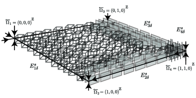
Figure 1: Plane fields $E_{i}^{s}$ in the example given by $f\colon(x,y,z)\mapsto(x^{2},y^{2},0)$.

Remark 6.2.

From the definition given in §6.1, Property $(iii)$ means that for every $i$, for every compact subset $C$ of $W^{s}(\overleftarrow{\Omega}_{i})$, for every $\epsilon>0$, there exists a compact neighborhood $U$ of $C$ in $V_{i}$ such that for every $\delta$ sufficiently small

$$d_{H}(Graph(E_{i}^{s}|U),Graph(E^{s}|C))\leq\epsilon,$$

where $d_{H}(\cdot,\cdot)$ denotes the Hausdorff distance of compact subsets of $\overleftarrow{M}_{f}\times G_{N}$ induced by the distance $d_{1}+d_{G}$. We notice that $U$ depends on $C$ and $\epsilon$ but not on $\delta$ small enough.

Remark 6.3.

Property $(iv)$ means that $E_{i}^{s}$ is of constant dimension, $d_{1}$-continuous, and that for every compact subset $C$ of $V_{i}$ there exists a constant $L_{C}^{\delta}$ such that:

$$d_{G}(E_{i\underline{x}}^{s},E_{i\underline{y}}^{s})\leq L_{C}^{\delta}d_{\infty}(\underline{x},\underline{y}),\quad\forall\underline{x},\underline{y}\in C.$$

In the diffeomorphism case, to obtain the existence of $(E^{u}_{i\delta})_{i}$ it suffices to first push forward by $F^{\delta}$ each of the plane field $E^{s}_{i}$ on $\cup_{n}\overleftarrow{f}^{n}(V_{i})$ (which is a neighborhood of $W^{u}(\overleftarrow{\Omega}_{i})$, and then to apply the same proposition to $\overleftarrow{f}^{-1}$. In our case, even though $\overleftarrow{f}$ is invertible, the bundle map $F^{0}$ is not. However, in Lemma 3.4, we saw that $F^{\delta}$ is invertible for every $\delta>0$. Nonetheless, the norm of the inverse of this map depends on $\delta$, and so the angle between $E_{i}^{s}$ and $E_{i}^{u}$ as well. However in Proposition 4.1 such an angle must be bounded by a constant which is independent of $\delta$ (and this is necessary in the proof of Proposition 3.6).

Hence we must redo a similar construction, still in a neighborhood of each $W^{s}(\overleftarrow{\Omega}_{i})$ since it is the only place where we control the singularities.

Another difference in the construction of $E_{i}^{u}$ is the following: to construct the plane field $E_{i}^{u}$ we will not be allowed to pull back, since the critical set might intersect $W^{s}(\overleftarrow{\Omega}_{i})$, and a pull back by $F^{0}$ would contain critical vectors which belong to $E^{s}$, this would contradict the angle condition $(iii)$ for $\delta>0$. Hence the construction of $E_{i}^{u}$ must be done in compact set in a small neighborhood of $W^{s}(\overleftarrow{\Omega}_{i})$ via push forward.

Proposition 6.4.

There exist $K>0$, an open cover $(W_{i})_{i=1}^{q}$ of $\overleftarrow{M}_{f}$, where each $W_{i}$ contains $\overleftarrow{\Omega}_{i}$ and is included in $V_{i}$, such that for every $\delta>0$, there exists a subbundle $E_{i}^{u}$ of $W_{i}\times\mathbb{R}^{N}\to W_{i}$ satisfying the following properties for $i\in[1,q]$:

1. For every $\underline{x}\in W_{i}\cap\overleftarrow{f}^{-1}(W_{i})$, the map $F^{\delta}$ sends $E_{i\underline{x}}^{u}$ into $E_{i\overleftarrow{f}(\underline{x})}^{u}$.

2. For every $j\geq i$, for every $\underline{x}\in W_{i}\cap\overleftarrow{f}^{-1}(W_{j})$ the following inclusion holds:

   $$F^{\delta}(E_{j{\underline{x}}}^{u})\supset E_{i\overleftarrow{f}({\underline{x}})}^{u}.$$

3. $E^{s}_{i\underline{x}}\oplus E^{u}_{i\underline{x}}=\mathbb{R}^{N}$, for every $\underline{x}\in W_{i}$, the angle between $E_{i}^{s}$ and $E_{i}^{u}$ is bounded from below by $K^{-1}$.

4. The subbundle $E_{i}^{u}$ is of constant dimension, $d_{1}$-continuous and $d_{\infty}$-Lipschitz.

5. For every $\underline{x}\in W_{i}$, it holds

   $$\|{F^{\delta}}(v^{u})\|\geq\|v^{u}\|/K,\quad\forall v^{u}\in E^{u}_{i\underline{x}}.$$

6. For every $q^{\prime}$, if $\underline{x}\in W_{q^{\prime}}$ then $\overleftarrow{f}(\underline{x})\notin\cup_{j>q^{\prime}}W_{j}$ and $\cap_{n\in\mathbb{Z}}\overleftarrow{f}^{n}(W_{q^{\prime}})=\overleftarrow{\Omega}_{q^{\prime}}$.

Figure 2 depicts an example of such plane fields.

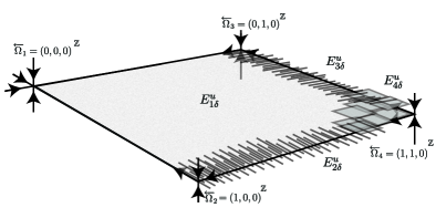
Figure 2: Plane fields $E_{i}^{u}$ in the example given by $f\colon(x,y,z)\mapsto(x^{2},y^{2},0)$.

From the two latter propositions, we easily deduce:

Proof of Proposition 4.1.

By Propositions 6.1 and 6.4, we have immediately properties $(i)$-$(ii)$-$(iii)$-$(iv)$-$(v)$-$(vi)$ of Proposition 4.1. To prove property $(vii)$, we remark that by Proposition 6.1 $(i)$ and $(iii)$ together with the hyperbolicity of $\overleftarrow{\Omega}$, the bundle $E^{s}_{i}$ is contracted by $F^{\delta}$ over a neighborhood of $\overleftarrow{\Omega}_{i}$, for every $i$. Moreover, by properties $(i)$-$(iii)$-$(iv)$ of Proposition 6.4, the bundle $E^{u}_{i}$ is close to $E^{u}|\overleftarrow{\Omega}_{i}$, and so expanded by $F^{\delta}$ on a neighborhood of $\overleftarrow{\Omega}_{i}$ (see Proposition 1.2). ∎

7 Proof of Proposition 6.1

Let us recall that $(M_{j})_{j=1}^{q}$ is a filtration adapted $(\overleftarrow{\Omega}_{j})_{i=1}^{q}$ (see §4 for details). An example of such a filtration is depicted figure 3.

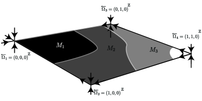
Figure 3: A filtration for the example given by $f\colon(x,y,z)\mapsto(x^{2},y^{2},0)$.

We are going to construct $(E_{i}^{s})_{i}$ by (increasing) induction on $i$. Here it is the induction hypothesis at the step $i$:

For every $N_{i}\leq 0$, there exist neighborhoods $(V_{j}^{i})_{j=1}^{i}$ of respectively $(W^{s}(\overleftarrow{\Omega}_{j})\cap\overleftarrow{f}^{N_{i}}(M_{i}))_{j=1}^{q}$ in $\overleftarrow{f}^{N_{i}}(M_{i})$, there are functions

$$E_{j}^{s}\colon V_{j}^{i}\to G_{N}$$

which satisfy the following properties for every $j\leq i$:

1. for every ${\underline{x}}\in V^{i}_{j}\cap\overleftarrow{f}^{-1}(V^{i}_{j})$ the following inclusion holds:

   $$F^{\delta}(E_{j{\underline{x}}}^{s})\subset E_{j\overleftarrow{f}({\underline{x}})}^{s}.$$

2. for every $k\geq j$, for every ${\underline{x}}\in V^{i}_{k}\cap V^{i}_{j}$ the following inclusion holds:

   $$E_{k{\underline{x}}}^{s}\subset E_{j{\underline{x}}}^{s}.$$

3. $E_{j}^{s}$ is compact-open close to $E^{s}|W^{s}(\Omega_{j})\cap V_{j}^{i}$, when $\delta$-is small.

4. $E_{j}^{s}$ is of constant dimension, $d_{1}$-continuous, and locally Lipschitz for the metric $d_{\infty}$.

We remark that the step $i=q$ gives the statement of Proposition 6.1 with $V_{i}:=\overleftarrow{f}^{-1}(V_{i}^{q})\cap V_{i}^{q}$ for every $i$.

We recall that each $E_{j}^{s}$ depends on $\delta$. During several parameters will be fixed.

The order is the following at the step $i$. First an arbitrary negative integer $N_{i}$ is given. Then $\eta>0$ is chosen. Depending on $N_{i}$ and $\eta$, we will suppose $\delta$ small. The induction hypothesis is used with $\delta$ and $N_{i-1}$ chosen large in function of $N_{i}$ and $\eta$.

Step $i=1$

Let $N_{1}\leq 0$, and put $K_{1}:=\overleftarrow{f}^{N_{1}}(M_{1})$. We notice that $W^{s}(\overleftarrow{\Omega}_{1})$ is an open set of $\overleftarrow{M}_{f}$. Hence we put $V_{1}^{1}:=K_{1}$. Note that $\overleftarrow{f}(K_{1})\subset K_{1}$.

Let $K_{1}\ni\underline{x}\mapsto E^{\prime}_{\underline{x}}$ be the restriction to $K_{1}$ of a smooth approximation of the continuous map $E^{s}|W^{s}(\overleftarrow{\Omega}_{1})\colon W^{s}(\overleftarrow{\Omega}_{1})\to G_{N}$ given by Corollary 5.3.

Observe that $E^{\prime}$ is uniformly close to $E^{s}|K_{1}$. Moreover it is $d_{1}$-continuous and $d_{\infty}$-Lipschitz. We recall that the Banach manifold $C^{0}(K_{1},G_{N})$ was defined in §6.1.

For all $\eta>0$ and $\delta>0$, the following is well defined on the closed ball $\bar{B}_{C^{0}}(E^{\prime},\eta)\subset C^{0}(K_{1},G_{N})$ with image in $C^{0}(K_{1},G_{N})$.

$$F^{\delta\#}:=\bar{B}_{C^{0}}(E^{\prime},\eta)\ni P\mapsto\left[\underline{x}\mapsto F_{x_{0}}^{\delta^{-1}}(P_{\overleftarrow{f}(\underline{x})})\right],\quad\text{with }x_{0}:=\pi_{0}(\underline{x}).$$

By hyperbolicity, for $\delta$ small enough and $E^{\prime}$ sufficiently close to $E^{s}$, there exists some $k\in\mathbb{N}$ such that ${F^{\delta\#}}^{k}$ is $\lambda$-contracting and sends the closed ball $\bar{B}_{C^{0}}(E^{\prime},\eta)$ into itself.

Let $E_{1}^{s}$ be the unique fixed point of $F^{\delta\#}$ in $B_{C^{0}}(E^{\prime},\eta)$. By definition, condition $(i)$ is satisfied.

Condition $(iii)$ follows from the fact that $\eta$ can be taken small when $\delta$ is small.

It remains only to show that $(iv)$ holds. First let us recall that $E^{s}_{1}\in B_{C^{0}}(E^{\prime},\eta)$ and $x_{0}\in M\mapsto F^{\delta}_{x_{0}}\in L_{N}(\mathbb{R})$ is of class $C^{1}$, and so, $K_{1}\ni\underline{x}\mapsto F^{\delta}_{x_{0}}$ is $d_{\infty}$-Lipschitz. Since $F^{\delta}$ is moreover invertible, there exists $L_{\delta,k}$ such that for all $\underline{x},\underline{y}\in K_{1}$ and $P\in B_{C^{0}}(E^{\prime},\eta)$ it holds

$$d\big{(}{F^{\delta k}_{\underline{x}}}^{-1}(P_{\overleftarrow{f}^{k}(\underline{y})}),{F^{\delta k}_{\underline{y}}}^{-1}(P_{\overleftarrow{f}^{k}(\underline{y})})\big{)}\leq L_{\delta,k}d_{\infty}(\underline{x},\underline{y}),$$ (19)

where ${F^{\delta k}_{\underline{x}}}:={F^{\delta}_{x_{k-1}}}\circ\cdots\circ F^{\delta}_{x_{0}}$ and $x_{i}:=\pi_{i}(\underline{x})$ the $i^{th}$ coordinate of $\underline{x}$.

On the other hand, the map ${F^{\delta\#}}^{k}$ is pointwise $\lambda$-contracting:

$$d\big{(}{F^{\delta k}_{\underline{x}}}^{-1}(P_{\overleftarrow{f}^{k}(\underline{x})}),{F^{\delta k}_{\underline{x}}}^{-1}(P_{\overleftarrow{f}^{k}(\underline{y})})\big{)}\leq\lambda d(P_{\overleftarrow{f}^{k}(\underline{x})},P_{\overleftarrow{f}^{k}(\underline{y})}).$$ (20)

Consequently, adding (19) and (20) we get

$$d\big{(}{F^{\delta^{-k}}_{\underline{x}}}(P_{\overleftarrow{f}^{k}(\underline{x})}),{F^{\delta^{-k}}_{\underline{y}}}(P_{\overleftarrow{f}^{k}(\underline{y})}\big{)}\leq L_{\delta,k}d_{\infty}(\underline{x},\underline{y})+\lambda d(P_{\overleftarrow{f}^{k}(\underline{x})},P_{\overleftarrow{f}^{k}(\underline{y})}).$$ (21)

For every $d_{\infty}$-Lipschitz distribution $P$ let us denote by $\Lambda(P)$ its Lipschitz constant. It holds for every $k$:

$$d(P_{\overleftarrow{f}^{k}(\underline{x})},P_{\overleftarrow{f}^{k}(\underline{y})})\leq\Lambda(P)d_{\infty}(\underline{x},\underline{y}).$$ (22)

Thus by (21) and (22):

$$d\big{(}{F^{\delta k}}^{-1}_{\underline{x}}(P_{\overleftarrow{f}^{k}(\underline{x})}),{F^{\delta k}}^{-1}_{\underline{y}}(P_{\overleftarrow{f}^{k}(\underline{y})}\big{)}\leq(L_{\delta,k}+\lambda\Lambda(P))d_{\infty}(\underline{x},\underline{y})$$

Consequently the closed subset of $B_{C^{0}}(E^{\prime},\eta)$ formed by sections with $d_{\infty}$-Lipschitz constant smaller or equal than any $\Lambda\geq(1-\lambda)^{-1}L_{\delta,k}$ is forward invariant under ${F^{\delta\#}}^{k}$. We recall that $E^{\prime}$ is $d_{\infty}$-Lipschitz. Hence if $\Lambda\geq\Lambda(E^{\prime})$, this subset is non empty (it contains $E^{\prime}$), thus there exists a fixed point $d_{\infty}$-Lipschitz in $\bar{B}_{C^{0}}(E^{\prime},\eta)$. By uniqueness, the fixed point $K_{1}\ni\underline{x}\mapsto E^{s}_{1\underline{x}}\in G_{N}$ is $d_{\infty}$-Lipschitz.

$\square$

Step $i-1\rightarrow i$

Let $N_{i}$ be an arbitrary negative integer. Put:

$$K_{i}:=W^{s}(\overleftarrow{\Omega}_{i})\cap\overleftarrow{f}^{N_{i}}(M_{i}).$$

Let us begin as in the step $i=1$.

We can extend $d_{1}$-continuously the section $E^{s}|K_{i}\colon K_{i}\to G_{N}$ to an open neighborhood of $K_{i}$. Let $\underline{x}\mapsto E^{\prime}_{\underline{x}}$ be a smooth approximation given by Corollary 5.3 of such a continuous extension.

The section $E^{\prime}$ is well defined on a small neighborhood $Z_{i}$ of $K_{i}$ in $\overleftarrow{f}^{N_{i}}(M_{i})$ of the form:

$$Z_{i}:=\overleftarrow{f}^{N_{i}}(M_{i})\setminus int\,\overleftarrow{f}^{N_{i-1}+1}(M_{i-1}),\quad N_{i-1}\leq 0$$

Indeed note that $K_{i}=\overleftarrow{f}^{N_{i}}(M_{i})\setminus\cup_{n\leq 0}\overleftarrow{f}^{n}(M_{i-1})$, so $Z_{i}$ is close to $K_{i}$ whenever $-N_{i-1}$ is large enough (see fig. 4).

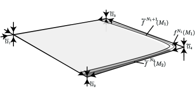
Figure 4: Construction of $Z_{2}=f^{N_{2}}(M_{2})\setminus int\,f^{N_{1}+1}(M_{1})$ in the example given by $f\colon(x,y,z)\mapsto(x^{2},y^{2},0)$.

Observe that $E^{\prime}|K_{i}$ is $C^{0}$-close to $E^{s}|K_{i}$, $d_{1}$-continuous and $d_{\infty}$-Lipschitz.

Hence, for every $\eta$ small, for every $Z_{i}$ and $\delta$ small enough, for $E^{\prime}$ sufficiently close to $E^{s}$, the following is well defined on the ball $\bar{B}_{C^{0}}(E^{\prime},\eta)\subset C^{0}(Z_{i},G_{N})$ with image in $C^{0}(Z_{i}\cap\overleftarrow{f}^{-1}(Z_{i}),G_{N})$:

$$F^{\delta\#}:=\bar{B}_{C^{0}}(E^{\prime}|Z_{i},\eta)\ni P\mapsto\left[Z_{i}\cap\overleftarrow{f}^{-1}(Z_{i})\ni\underline{x}\mapsto F_{x_{0}}^{\delta^{-1}}(P(\overleftarrow{f}(\underline{x})))\right].$$

By hyperbolicity, for $\eta$ small and then for $Z_{i}$ and $\delta$ small enough and $E^{\prime}$ sufficiently close to $E^{s}$, there exist some $k\in\mathbb{N}$, such that the following map:

$${F^{\delta\#}}^{k}:=\bar{B}_{C^{0}}(E^{\prime}|Z_{i},\eta)\ni P\mapsto\left[\bigcap_{0\leq l\leq k}\overleftarrow{f}^{-l}(Z_{i})\ni\underline{x}\mapsto{F_{x_{0}}^{\delta}}^{-k}(P(\overleftarrow{f}^{k}(\underline{x})))\right].$$

is contracting and sends the closed ball $\bar{B}_{C^{0}}(E^{\prime}|Z_{i},\eta)$ into $\bar{B}_{C^{0}}(E^{\prime}|\cap_{l\leq k}\overleftarrow{f}^{-l}(Z_{i}),\eta)$.

As the target space is not the same as the source space, we cannot conclude to the existence of a fixed point. We are going to extend the sections in the image of ${F^{\delta\#}}$ by a section constructed by the following lemma shown below:

Lemma 7.1.

There exist a sequence of negative integers $(N_{j})_{j<i-1}$ and a section $\tilde{E}\in B_{C^{0}}(E^{\prime}|Z_{i},\eta/2)$ which is $d_{1}$-continuous and $d_{\infty}$-Lipschitz such that for every $j<i$:

1. $Z_{j}:=\overleftarrow{f}^{N_{j}}(M_{j})\setminus int\,\overleftarrow{f}^{N_{j-1}+1}(M_{j-1})\subset int\,V_{j}^{i-1}.$

2. $\forall\underline{x}\in Z_{j}\cap Z_{i},\quad\tilde{E}(\underline{x})\subset E_{j}^{s}(\underline{x})$.

Gluing $\tilde{E}$ to $F^{\delta\#}\tilde{E}$ and definition of $E_{i}^{s}$

We remark that $\tilde{E}$ and $F^{\delta\#}\tilde{E}$ are well defined on:

$$V_{i}^{i}:=\overleftarrow{f}^{N_{i}}(M_{i})\setminus\overleftarrow{f}^{N_{i-1}}(M_{i-1}).$$

By Corollary 5.2, there exists a partition of the unity $(\rho,1-\rho)\in\mathrm{Mor}_{0}^{\infty}(\overleftarrow{M}_{f})^{2}$ subordinated to the cover $(\overleftarrow{f}^{N_{i-1}-1}(int\,M_{i-1}),\overleftarrow{M}_{f}\setminus\overleftarrow{f}^{N_{i-1}}(M_{i-1}))$.

For $\underline{x}\in V_{i}^{i}$, let $p_{\underline{x}}$ and $p^{\prime}_{\underline{x}}$ be the orthogonal projections of $\mathbb{R}^{N}$ onto respectively $\tilde{E}(\underline{x})$ and $F^{\#}\tilde{E}(\underline{x})$. Put

$$E^{0}(\underline{x}):=\{(\rho(\underline{x})p_{\underline{x}}+(1-\rho(\underline{x}))p^{\prime}_{\underline{x}})(u);\;u\in\tilde{E}(\underline{x})\}.$$

We notice that $V_{i}^{i}\ni\underline{x}\mapsto E^{0}(\underline{x})\in G_{N}$ is $d_{1}$-continuous and $d_{\infty}$-Lipschitz. Furthermore, for $\underline{x}\in V_{i}^{i}$ close to $\overleftarrow{f}^{N_{i-1}}(M_{i-1})$, the plane $E^{0}(\underline{x})$ is equal to $\tilde{E}(\underline{x})$ and for $\underline{x}\in V_{i}^{i}\setminus\overleftarrow{f}^{N_{i-1}-1}(int\,M_{i-1})$, the plane $E^{0}(\underline{x})$ is equal to $F^{\delta\#}\tilde{E}_{\underline{x}}$.

We define

$$\Pi_{\eta}:=\{P\in C^{0}(V_{i}^{i},G_{N}):\;P=E^{0}\;\text{on}\;V_{i}^{i}\setminus\overleftarrow{f}^{N_{i-1}-1}(M_{i-1})\text{ and}\\ \text{the restriction }P\text{ and }E^{\prime}\text{ to }\cap_{j=0}^{k}\overleftarrow{f}^{j}(V_{i}^{i})\text{ are }\eta-C^{0}-\text{close}\}.$$

We remark that the following map is continuous.

$$F^{\delta\star}:=P\in\Pi_{\eta}\mapsto\left[V_{i}^{i}\ni\underline{x}\mapsto\left\{\begin{array}[]{cl}E^{0}(\underline{x})&\text{if }\underline{x}\in V_{i}^{i}\setminus\overleftarrow{f}^{N_{i-1}-1}(M_{i-1})\\ {F^{\delta}}_{\underline{x}}^{-1}(P(\overleftarrow{f}(x)))&\text{otherwise.}\end{array}\right.\right]$$

As ${F^{\delta\#}}^{k}$ is contracting and sends $\bar{B}_{C^{0}}(E^{\prime}|Z_{i},\eta)$ into $\bar{B}_{C^{0}}(E^{\prime}|\cap_{j}\overleftarrow{f}^{j}(Z_{i}),\eta)$, the map $F^{\delta\star^{k}}$ is contracting and sends $\Pi_{\eta}$ into itself.

Let $E_{i}^{s}$ be the fixed point of $F^{\delta\star}$.

By definition, $E_{i}^{s}$ satisfies property $(i)$. Similarly to the step $i=1$, the section $E_{i}^{s}$ satisfies Properties $(iii)$ and $(iv)$. However all the sections $(E_{j}^{s})_{j\leq i}$ need to be extended from $(V_{j}^{i-1})_{j\leq i}$ to $(V_{j}^{i})_{j\leq i}$ which remains to be constructed.

Construction of $(V_{j}^{i})_{j\leq i}$ and extension of $(E_{j}^{s})$

For every $j<i$, we recall that for every $\underline{x}\in Z_{j}\cap Z_{i}$, the plane $\tilde{E}_{\underline{x}}$ is included in $E^{s}_{j\underline{x}}$. By induction hypothesis $(i)$ and since $V_{i}^{i}=Z_{i}\cap\overleftarrow{f}^{-1}(Z_{i})$, for every $\underline{x}\in Z_{j}\cap V^{i}_{i}$, the plane $F^{\delta\#}\tilde{E}_{\underline{x}}$ is included in $E^{s}_{j\underline{x}}$. Hence, for every $\underline{x}\in Z_{j}\cap V^{i}_{i}$, the plane $E^{0}_{\underline{x}}$ is included in $E^{s}_{j\underline{x}}$. Again by induction hypothesis $(i)$, since the fixed point $E^{s}_{i\underline{x}}$ of $F^{\star}$ is obtained by iterating it, for every $\underline{x}\in Z_{j}\cap V^{i}_{i}$, the plane $E^{s}_{i\underline{x}}$ is included in $E^{s}_{j\underline{x}}$. Put

$$\tilde{V}_{j}:=V_{j}^{i-1}\cap\cup_{l=j}^{i-1}Z_{l}$$

By induction hypothesis $(ii)$, for every $\underline{x}\in\tilde{V}_{j}\cap V^{i}_{i}$, the plane $E^{s}_{i\underline{x}}$ is included in $E^{s}_{j\underline{x}}$. Using that $Z_{j}=\overleftarrow{f}^{N_{j}}(M_{j})\setminus int\,\overleftarrow{f}^{N_{j-1}+1}(M_{j-1})$, we remark that:

$$\tilde{V}_{j}\supset V_{j}^{i-1}\cap\overleftarrow{f}^{N_{i-1}}(M_{i-1})\setminus int\,\overleftarrow{f}^{N_{j-1}+1}(M_{j-1})=V_{j}^{i-1}\setminus int\,\overleftarrow{f}^{N_{j-1}+1}(M_{j-1}).$$

Hence $\tilde{V}_{j}$ is a neighborhood of $W^{s}(\overleftarrow{\Omega}_{j})\cap\overleftarrow{f}^{N_{i-1}}(M_{i-1})$ since $W^{s}(\overleftarrow{\Omega}_{j})$ does not intersect $\overleftarrow{f}^{N_{j-1}+1}(M_{j-1})$. Put

$$V_{j}^{i}:=\cup_{n\geq 0}(\overleftarrow{f}|V_{i}^{i})^{-n}(\tilde{V}_{j})\quad\text{where}\quad V_{i}^{i}=\overleftarrow{f}^{N_{i}}(M_{i})\setminus\overleftarrow{f}^{N_{i-1}}(M_{i-1})$$

Lemma 7.2.

For every $j\leq i$, the set $V_{j}^{i}$ is a neighborhood of $W^{s}(\Omega_{j})\cap f^{N_{i}}(M_{i})$ in $f^{N_{i}}(M_{i})$.

Proof.

As the case $i=j$ is obvious, we suppose $j<i$. For every $\underline{x}\in f^{N_{i}}(M_{i})\cap W^{s}(\overleftarrow{\Omega}_{j})$ there exists $n$ such that $\overleftarrow{f}^{n}(\underline{x})\in int(f^{N_{i-1}}(M_{i-1}))$. Consequently, for every $\underline{y}\in\overleftarrow{f}^{N_{i}}(M_{i})$ nearby $\underline{x}$, there exists $m$ such that $\overleftarrow{f}^{m}(\underline{y})\in\overleftarrow{f}^{N_{i-1}}(M_{i-1})$. Let us consider such an $m$ minimal. Since $\tilde{V}_{j}$ is a neighborhood of $W^{s}(\overleftarrow{\Omega}_{j})\cap f^{N_{i-1}}(M_{i-1})$ in $f^{N_{i-1}}(M_{i-1})$, the point $\overleftarrow{f}^{m}(\underline{y})$ belongs to $\tilde{V}_{j}$ for $\underline{y}$ sufficiently close to $\underline{x}$ . Also for every $k<m$ the point $\overleftarrow{f}^{k}(\underline{y})$ belongs to the complement of $f^{N_{i-1}}(M_{i-1})$. On the other hand, $\overleftarrow{f}^{k}(\underline{y})$ belongs to $f^{N_{i}}(M_{i})$ for every $k$. Thus for every $k<m$, the point $\overleftarrow{f}^{k}(\underline{y})$ belongs to $V_{i}^{i}=\overleftarrow{f}^{N_{i}}(M_{i})\setminus\overleftarrow{f}^{N_{i-1}}(M_{i-1})$. As $\overleftarrow{f}^{m}(\underline{y})$ belongs to $\tilde{V}_{j}$, it follows that $\underline{y}$ belongs to $V_{j}^{i}$.∎

We extend $E_{j}^{s}$ on $V_{j}^{i}$ by:

$$\forall x\in V_{j}^{i},\forall n\geq 0\text{ minimal such that }\overleftarrow{f}^{n}(\underline{x})\in\tilde{V}_{j},\;E_{j\underline{x}}^{s}={F_{\underline{x}}^{\delta}}^{-n}(E_{j\overleftarrow{f}^{n}(\underline{x})}^{s}).$$

Induction hypotheses $(i)$, $(iii)$ and $(iv)$ for $j<i$ imply properties $(i)$, $(iii)$ and $(iv)$ for $E_{j}^{s}$ on $V_{j}^{i}$.

Let us check property $(ii)$. As this property is invariant by pull back, property $(i)$ implies that property $(ii)$ holds for every $k\leq j$ both less than $i$. Let $\underline{x}\in V_{i}^{i}\cap V_{j}^{i}$. Let $n$ be such that $\underline{x}$ belongs to $\overleftarrow{f}^{-n}(\tilde{V}_{j})\cap V_{i}^{i}$. We recall that $V_{i}^{i}=\overleftarrow{f}^{N_{i}}(M_{i})\setminus\overleftarrow{f}^{N_{i-1}}(M_{i-1})$, hence $\overleftarrow{f}^{n}(\underline{x})$ belongs to $\overleftarrow{f}^{N_{i}+n}(M_{i})\subset\overleftarrow{f}^{N_{i}}(M_{i})$. Also $\overleftarrow{f}^{n}(\underline{x})$ belongs to $\tilde{V}_{j}\subset V_{j}^{i-1}\subset f^{N_{i-1}}(M_{i-1}^{c})$. Thus $\overleftarrow{f}^{n}(\underline{x})\in\tilde{V}_{j}\cap V_{i}^{i}$. Consequently, Property $(ii)$ holds at $\overleftarrow{f}^{n}(\underline{x})$. By pull back invariance and property $(i)$, Property $(ii)$ holds at $\underline{x}$.

Proof of Lemma 7.1

We are going to project $E^{\prime}$ onto each $E^{s}_{j}$, $j\leq i$. The following is a consequence of the Lambda-lemma and the strong transversality condition.

Claim 7.1.

For $Z_{i}$ small enough (that is $-N_{i-1}$ large enough), for $\delta$ small enough, for every $j<i$, every $\underline{x}\in W^{s}(\overleftarrow{\Omega}_{j})\cap Z_{i}$, if $q_{j}(\underline{x})$ denotes the orthogonal projection of $\mathbb{R}^{N}$ onto $E^{s}_{\underline{x}}$, the distance between $q_{j}(\underline{x})(E^{\prime}_{\underline{x}})$ and $E^{\prime}_{\underline{x}}$ is less than $\eta/4i$.

Proof.

By the strong transversality condition, on $W^{u}_{\epsilon}(\overleftarrow{\Omega}_{i})\setminus\overleftarrow{\Omega}_{i}$ the stable direction $E^{s}$ is transverse to $TW^{u}_{\epsilon}(\overleftarrow{\Omega}_{i})$. This is true in particular on $W^{u}_{\epsilon}(\overleftarrow{\Omega}_{i})\cap W^{s}(\overleftarrow{\Omega}_{j})$. By hyperbolicity and the strong transversality condition, for every $(\underline{x}_{n})_{n}$ in $W^{u}_{\epsilon}(\overleftarrow{\Omega}_{i})\cap W^{s}(\overleftarrow{\Omega}_{j})$ approaching $\underline{x}\in\Omega_{i}$, every accumulation plane $P$ of $(E^{s}_{\underline{x}_{n}})_{n}$ contains the plane $E^{s}_{\underline{x}}$. This implies that for every $(\underline{x}_{n})_{n}$ in $W^{s}(\overleftarrow{\Omega}_{j})$ approaching $\underline{x}\in K_{i}=\overleftarrow{f}^{N_{i}}(M_{i})\cap W^{s}(\overleftarrow{\Omega}_{i})$, every accumulation plane $P$ of $(E^{s}_{\underline{x}_{n}})_{n}$ contains the plane $E^{s}_{\underline{x}}$. The claim follows since $E^{\prime}$ is close to $E^{s}|K_{i}$ for $\delta$ small and $Z_{i}$ small. ∎

We will perform orthogonal projections of $E^{s}_{i}$ on compact subsets of each $Z_{i}\cap W^{s}(\overleftarrow{\Omega}_{j})$.

Let us implement these compact subsets.

First let us notice that $cl(Z_{i}\setminus\overleftarrow{f}^{-1}(Z_{i}))$ is a compact subset of $\cup_{j<i}W^{s}(\Omega_{j})$:

$$Z_{i}\setminus\overleftarrow{f}^{-1}(Z_{i})=\overleftarrow{f}^{N_{i}}(M_{i})\setminus int\,\overleftarrow{f}^{N_{i-1}+1}(M_{i-1})\setminus\big{(}\overleftarrow{f}^{N_{i}-1}(M_{i})\setminus int\,\overleftarrow{f}^{N_{i-1}}(M_{i-1})\big{)}.$$

As $\overleftarrow{f}^{N_{i}}(M_{i})$ is included in $\overleftarrow{f}^{N_{i}-1}(M_{i})$ it comes:

$$Z_{i}\setminus\overleftarrow{f}^{-1}(Z_{i})=\overleftarrow{f}^{N_{i}}(M_{i})\cap int\,\overleftarrow{f}^{N_{i-1}}(M_{i-1})\setminus int\,\overleftarrow{f}^{N_{i-1}+1}(M_{i-1})\subset\cup_{j<i}W^{s}(\overleftarrow{\Omega}_{j}).$$

Let $(V_{k}^{i-1})_{k\leq i-1}$ be the neighborhoods given by the induction hypothesis at step $i-1$ for the integer $N_{i-1}$ defined above.

By decreasing induction we construct $(N_{k})_{k=1}^{i-2}\in\mathbb{Z}^{-}$ such that, the following holds.

Claim 7.2.

For every $k\leq i-1$, the set $Z_{k}:=\overleftarrow{f}^{N_{k}}(M_{k})\setminus\overleftarrow{f}^{N_{k-1}+1}(M_{k-1})$ has its closure included in the interior of $V_{k}^{i-1}$. Moreover, for $\delta$ small enough, the distance between the orthogonal projection $p_{k}$ onto $E^{s}_{k}$ satisfies:

$$\|p_{k}(\underline{x})(E^{\prime}_{\underline{x}})-E^{\prime}_{\underline{x}}\|\leq\eta/3i,\quad\forall\underline{x}\in Z_{k}.$$ (23)

,

Proof.

For $k\leq i-1$, suppose $N_{k}$ constructed. Then for $-N_{k-1}$ large, the set $Z_{k}$ is close to the compact set $W^{s}(\overleftarrow{\Omega}_{k})\cap f^{N_{k}}(M_{k})$, and so it is included in $V_{k}$. Moreover, by remark 6.3 and Claim 7.1 for $-N_{k-1}$ large and $\delta$ small, inequality (23) holds.∎

Let $\hat{Z}_{k}$ be a neighborhood of $Z_{k}$ in $V_{k}^{i-1}$ such that for all $\underline{x}\in\hat{Z}_{k}$,

$$\|p_{k}(\underline{x})(E^{\prime}_{\underline{x}})-E^{\prime}_{\underline{x}}\|\leq\frac{\eta}{2i}.$$

By corollary 5.2, there exists a dump function $\rho\in Mor_{0}^{\infty}(\overleftarrow{f}^{N_{i-1}}(M_{i-1}),[0,1])$ equal to $1$ on $Z_{k}$ and to $0$ on $\hat{Z}_{k}^{c}$. We construct $(P_{\underline{x}}^{j})_{j<i}$ by induction. Put $P^{0}=E^{\prime}$, and for $j\in[1,i-1]$ put

$$P_{\underline{x}}=\{\rho_{j}(\underline{x})\cdot q_{j}(\underline{x})(u)+(1-\rho_{j}(\underline{x}))\cdot u:\;u\in P_{\underline{x}}^{j-1}\}$$

Let $\hat{E}=P_{\underline{x}}^{i-1}$. By induction hypothesis $(ii)$, for every $\underline{x}\in Z_{i}\cap Z_{j}$, it holds $\tilde{E}_{\underline{x}}\subset E^{s}_{j\underline{x}}$.

By definition of $\hat{Z}_{k}$, the section $\tilde{E}$ is in $B_{C^{0}}(E^{\prime}|Z_{i},\eta/2)$ and is $d_{\infty}$-Lipschitz.

8 Proof Proposition 6.4

The proof of Proposition 6.4 is done by decreasing induction on $q^{\prime}\in[1,q]$. We recall that Proposition 6.1 constructed sections $(E_{j}^{s})_{j}$ on neighborhoods $(V_{j})_{j}$ of respectively $(W^{s}_{j}(\overleftarrow{\Omega}_{j}))_{j}$, which satisfy properties $(i)$-$(ii)$-$(iii)$ and $(iv)$. Here is the induction hypothesis.

For every $q^{\prime}\leq q$, there exist $K>0$ and an open cover $(W_{i})_{i=q^{\prime}}^{q}$ of $\cup_{j\geq q^{\prime}}W^{s}(\overleftarrow{\Omega}_{j})$, where each $W_{i}$ is a neighborhood of $\overleftarrow{\Omega}_{i}$ included in $V_{i}^{i}$ and such that for every $\delta>0$, there exists a function $E_{i}^{u}\in C^{0}(W_{i},G_{N})$ satisfying the following properties for $i\in[q^{\prime},q]$:

1. For every $\underline{x}\in W_{i}\cap\overleftarrow{f}^{-1}(W_{i})$, the map $F^{\delta}$ sends $E_{i\underline{x}}^{u}$ into $E_{i\overleftarrow{f}(\underline{x})}^{u}$.

2. For every $j\geq i$, for every $\underline{x}\in W_{i}\cap\overleftarrow{f}^{-1}(W_{j})$ the following inclusion holds:

   $$E_{i{\underline{x}}}^{u}\subset E_{j\overleftarrow{f}({\underline{x}})}^{u}.$$

3. $E^{s}_{i\underline{x}}\oplus E^{u}_{i\underline{x}}=\mathbb{R}^{N}$, for every $\underline{x}\in W_{i}$; the angle between $E_{i}^{s}$ and $E_{i}^{u}$ is bounded from below by $K^{-1}$.

4. The subbundle $E_{i}^{u}$ is of constant dimension, $d_{1}$-continuous and $d_{\infty}$-Lipschitz.

5. For any $\underline{x}\in W_{i}$, it holds

   $$\|{F^{\delta}}(v^{u})\|\geq\|v^{u}\|/K,\quad\forall v^{u}\in E^{u}_{i\underline{x}}.$$

6. It holds $cl(\overleftarrow{f}^{-1}(\cup_{q^{\prime}}^{q}W_{i}))\subset\cup_{q^{\prime}}^{q}W_{i}$. Moreover, for every $j\geq i$, if $\underline{x}\in W_{j}$ then $\overleftarrow{f}(\underline{x})\notin\cup_{k>j}W_{k}$ and $\cap_{n\in\mathbb{Z}}\overleftarrow{f}^{n}(W_{j})=\overleftarrow{\Omega}_{j}$.

We continue to denote by $(M_{j})_{j=1}^{q}$ a filtration adapted to $(\overleftarrow{\Omega}_{j})_{i=1}^{q}$ (see §4 for details and fig. 3).

At each step $q^{\prime}$ of the induction we will work with a small $\eta$ and we will suppose an integer $-N_{q^{\prime}}$ large and $\delta$ small both depending on $\eta$.

Step $q^{\prime}=q$

The subset $\overleftarrow{\Omega}_{q}=W^{s}(\overleftarrow{\Omega}_{q})$ is compact. Moreover there exists an arbitrarily small compact neighborhood $W_{q}$ of $\overleftarrow{\Omega}_{q}$ which satisfies $(vi)$ for $i=q$. Indeed, consider $W_{q}$ of the form $\overleftarrow{M}_{f}\setminus\overleftarrow{f}^{-N}(M_{q-1})$. Hence we can suppose that $W_{q}$ is included in $V_{q}$.

Let $\eta>0$ be small, in particular smaller than the angle between $E^{s}|\Omega(\overleftarrow{f})$ and $E^{u}|\Omega(\overleftarrow{f})$.

Let $\underline{x}\mapsto E^{\prime}_{\underline{x}}$ be the restriction to $W_{q}$ of a smooth approximation of a continuous extension of the continuous map $E^{u}|\overleftarrow{\Omega}_{q}\colon\overleftarrow{\Omega}_{q}\to G_{N}$ given by Corollary 5.3. This means that on the one hand, $E^{\prime}$ is $d_{1}$-continuous and $d_{\infty}$-Lipschitz, and that for every $\epsilon$ small, if $W_{q}$ is sufficiently small then for every $\underline{x}\in W_{q}$ there exists $\underline{y}\in\overleftarrow{\Omega}_{q}$ $\epsilon$-close to $\underline{x}$ such that the distance between $E^{\prime}_{\underline{x}}$ and $E^{u}_{\underline{y}}$ is $\eta$ small.

By hyperbolicity of $\overleftarrow{\Omega}_{q}$, the angle between $E^{s}_{\underline{y}}$ and $E^{u}_{\underline{y}}$ is uniformly bounded from below on $\underline{y}\in\overleftarrow{\Omega}_{q}$ and $Tf|E^{u}_{\underline{y}}$ is bijective. By property $(iii)$ of Proposition 6.1 and remark 6.2, there exists $K$ large such that for every $\eta>0$ small, for every $W_{q}$ sufficiently small, for all $\delta\geq 0$ small, and for every $\underline{y}\in W_{q}$ the following holds:

• the angle between $E^{s}_{q\underline{y}}$ and $E^{\prime}_{\underline{y}}$ is greater than $K^{-1}$,

• for every plane $P$ making an angle with $E^{\prime}_{\underline{y}}$ smaller than $\eta$, it holds:

  $$\forall u\in P,\quad\|F^{\delta}(u)\|\geq\|u\|/K.$$

Indeed, for $\underline{x}\in\overleftarrow{\Omega}_{q}$, every vector $u$ in $E^{u}$ is expanded by $F^{0}$.

We can now proceed as in the step $i=1$ of the proof of Proposition 6.1.

Since for every $\delta>0$, the map $F^{\delta}$ is bijective, the following is well defined

$$F_{\#}:=\bar{B}_{C^{0}}(E^{\prime},\eta)\ni P\mapsto\left[\underline{x}\mapsto F_{x_{0}}^{\delta}(P_{\overleftarrow{f}^{-1}(\underline{x})})\right]\in C^{0}(W_{q},G_{N}).$$

Moreover, for $\delta$, $W_{q}$ small enough and $E^{\prime}$ close enough to $E^{u}$, there exists some $k\in\mathbb{N}$ such that $F_{\#}^{k}$ is contracting and sends the closed ball $\bar{B}_{C^{0}}(E^{\prime},\eta)$ into itself.

Let $E_{q}^{s}$ be the unique fixed point of $F_{\#}$ in $B_{C^{0}}(E^{\prime},\eta)$. In this way, condition $(i)$ is clearly satisfied.

Properties $(iii)$ and $(v)$ follow from respectively Properties $(a)$ and $(b)$ above. Property $(ii)$ is empty.

To prove property $(iv)$, we proceed as in the proof of Proposition 6.1, step $i=1$.

$\square$

Step $q^{\prime}+1\rightarrow q^{\prime}$.

Let us suppose the neighborhoods $(W_{i})_{i=q^{\prime}+1}^{q}$ constructed so that

• property $(vi)$ holds,

• $W_{i}$ is a neighborhood of $\overleftarrow{\Omega}_{i}$,

Let us proceed again as in the proof of Proposition 6.1 step $i-1\rightarrow i$.

We remark that $C_{q^{\prime}}:=W^{s}(\overleftarrow{\Omega}_{q^{\prime}})\setminus\overleftarrow{f}^{-2}(O_{q^{\prime}})$ is compact, with $O_{q^{\prime}}:=\cup_{i=q^{\prime}+1}^{q}W_{i}$. Moreover for every $N_{q^{\prime}}\leq 0$, the following is a compact set containing $C_{q^{\prime}}$:

$$Y_{q^{\prime}}:=\overleftarrow{f}^{N_{q^{\prime}}}(M_{q^{\prime}-1}^{c})\setminus\overleftarrow{f}^{-2}(O_{q^{\prime}}),$$

Moreover, when $-N_{q^{\prime}}$ is large, $Y_{q^{\prime}}$ is close to $C_{q^{\prime}}$ for the Hausdorff metric. By $Y_{q^{\prime}}$ small we mean $-N_{q^{\prime}}$ large.

First, we assume $-N_{q^{\prime}}$ large enough so that the set $Y_{q^{\prime}}$ is included in $V_{q^{\prime}}$.

By strong transversality and property $(iii)$ of Proposition 6.1, for every $\eta>0$, there exists $K$ large such that for every $\delta$ and $Y_{q^{\prime}}$ small, it holds:

$$\forall\underline{x}\in Y_{q^{\prime}},\quad\forall u\in\mathbb{R}^{N}\setminus\{0\}:\quad|\angle(u,E_{q^{\prime}\underline{x}}^{s})|>\eta\Rightarrow\|F^{\delta}(u)\|\geq\|u\|/K.$$ (24)

Indeed, if $\underline{x}\in C_{q^{\prime}}$, a unit vector $u$ making an angle at least $\eta$ with $E_{\underline{x}}^{s}$ has its image by $F^{0}$ not in $E_{\overleftarrow{f}(\underline{x})}^{s}$, by the strong tranversality condition. Hence the norm if its image is bounded from below by a certain $1/2K$. Consequently for $\delta$ and $Y_{q^{\prime}}$ small inequality (24) holds.

For $\eta>0$, let $U_{\eta}$ be the closed subset of $C^{0}(Y_{q^{\prime}},G_{N})$ made by sections $P$ such that for every $\underline{x}\in Y_{q^{\prime}}$ the angle between $P_{\underline{x}}$ and $E_{q^{\prime}\underline{x}}^{s}$ is at least $\eta$.

For all $\eta$, $\delta$ and $Y_{q^{\prime}}$, the following is well defined with image in $C^{0}(Y_{q^{\prime}}\cap\overleftarrow{f}(Y_{q^{\prime}}),G_{N})$:

$$F_{\#}:=U_{\eta}\ni P\mapsto\left[\underline{x}\in Y_{q^{\prime}}\cap\overleftarrow{f}(Y_{q^{\prime}})\mapsto F_{x_{0}}^{\delta}(P_{\overleftarrow{f}^{-1}(\underline{x})})\right].$$

Similarly, for every $k\geq 0$, for all $\eta$, $\delta$ and $Y_{q^{\prime}}$, the following is well defined with image in $C^{0}(\cap^{k}_{i=0}\overleftarrow{f}^{i}(Y_{q^{\prime}}),G_{N})$:

$$F_{\#}^{k}:=U_{\eta}\ni P\mapsto\left[\underline{x}\in\cap^{k}_{i=0}\overleftarrow{f}^{i}(Y_{q^{\prime}})\mapsto{F_{x_{0}}^{\delta}}^{k}(P_{\overleftarrow{f}^{-k}(\underline{x})})\right].$$

We remark that $\cap^{k}_{i=0}\overleftarrow{f}^{i}(Y_{q^{\prime}})=f^{N_{q^{\prime}}}(M_{q^{\prime}-1}^{c})\setminus\overleftarrow{f}^{-2+k}(O_{q^{\prime}})$ is close to $\overleftarrow{\Omega}_{q^{\prime}}$, when $k$ is large and $Y_{q^{\prime}}$ is small (that is $-N_{q^{\prime}}$ large). We assume $\eta>0$ smaller than the angle between $E^{s}|\Omega_{q^{\prime}}$ and $E^{u}|\Omega_{q^{\prime}}$. Hence by hyperbolicity, for $Y_{q^{\prime}}$ and $\delta$ sufficiently small, there exists $k$ such that $F_{\#}^{k}$ is contracting for the $C^{0}$-metric. Note that $k$ does not depend on $\eta$. Moreover, by hyperbolicity, if $k$ is large enough and $\delta$ small enough, for every $\underline{x}\in\overleftarrow{f}^{k}(C_{q^{\prime}})$, for every $P_{\underline{x}}$ $\eta$-close to $E_{q^{\prime}\underline{x}}^{s}$, the plane ${F^{\delta}_{\underline{x}}}^{-k}(P_{\underline{x}})$ is $\eta$-close to $E^{s}_{\overleftarrow{f}^{-k}(\underline{x})}$. Hence every $\underline{x}\in C_{p}$, every $P$ making an angle greater than $\eta$ with $E^{s}_{\underline{x}}$, the plane ${F_{\underline{x}}^{\delta}}^{k}(P_{\underline{x}})$ makes an angle greater than $\eta$ with $E_{q^{\prime}\overleftarrow{f}^{k}(\underline{x})}^{s}$.

Consequently, for $-N_{q^{\prime}}$ large enough, $F_{\#}^{k}$ takes its values in the subspace of $C^{0}(\cap_{i=0}^{k}f^{i}(Y_{q^{\prime}}),G_{N})$ formed by sections $P$ such that for every $\underline{x}\in\cap_{i=0}^{k}f^{i}(Y_{q^{\prime}})$, $P_{\underline{x}}$ makes an angle with $E^{s}_{q^{\prime}\underline{x}}$ greater than $\eta>0$.

However, the target space of $F_{\#}$ is not the same as the source space. So we cannot conclude to a fixed point. We are going to complement the sections in the image of $F_{\#}$ by sections obtained by the following lemma shown below:

Lemma 8.1.

For $\delta$ and $Y_{q^{\prime}}$ small enough, there exists a $d_{1}$-continuous and $d_{\infty}$-Lipschitz section $\tilde{E}\in U_{\eta}$ such that for every $j>q^{\prime}$:

$$\underline{x}\in Y_{q^{\prime}}\cap\overleftarrow{f}(W_{j}),\quad\tilde{E}_{\underline{x}}\subset F^{\delta}(E_{j\overleftarrow{f}^{-1}(\underline{x})}^{u}).$$

Gluing $\tilde{E}$ to $F_{\#}\tilde{E}$ and definition of $E_{i}^{u}$

We remark that $\tilde{E}$ and $F_{\#}\tilde{E}$ are well defined on:

$$W_{q^{\prime}}:=\overleftarrow{f}^{N_{q^{\prime}}}(int\,M_{q^{\prime}-1}^{c})\setminus cl(\overleftarrow{f}^{-1}(O_{q^{\prime}}))\subset Y_{q^{\prime}}\cap\overleftarrow{f}(Y_{q^{\prime}}).$$

We remark that induction hypothesis $(vi)$ is satisfied.

By Corollary 5.2, there exists a partition of the unity $(\rho,1-\rho)\in Mor_{0}^{\infty}(\overleftarrow{M}_{f})^{2}$ subordinated to the cover $(O_{q^{\prime}},int\,\overleftarrow{f}^{-1}(O_{q^{\prime}})^{c})$.

Let $p_{\underline{x}}$ and $p^{\prime}_{\underline{x}}$ be the orthogonal projections of $\mathbb{R}^{N}$ onto respectively $\tilde{E}$ and $F_{\#}\tilde{E}$. For $\underline{x}\in W_{q^{\prime}}$, put

$$E^{0}_{\underline{x}}:=\{(\rho(\underline{x})p_{\underline{x}}+(1-\rho(\underline{x}))p^{\prime}_{\underline{x}})(u);\;u\in\tilde{E}_{\underline{x}}\}.$$

We notice that $\underline{x}\in W_{q^{\prime}}\mapsto E^{0}_{\underline{x}}\in G_{N}$ is $d_{1}$-continuous and $d_{\infty}$-Lipschitz. Furthermore, for $\underline{x}\in W_{q^{\prime}}$ close to $\overleftarrow{f}^{-1}(O_{q^{\prime}})$, the plane $E^{0}_{\underline{x}}$ is equal to $\tilde{E}_{\underline{x}}$ and for $\underline{x}\in W_{q^{\prime}}\setminus O_{q^{\prime}}$, the plane $E^{0}_{\underline{x}}$ is equal to $F_{\#}\tilde{E}_{\underline{x}}$.

We put

$$\Pi_{\eta}:=\{P\in C^{0}(W_{q^{\prime}},G_{N}):\;P=E^{0}\;\text{on}\;W_{q^{\prime}}\setminus O_{q^{\prime}}\text{ and}\\ P\text{ and }E_{q^{\prime}}^{s}\text{ makes an angle greater than }\eta\text{ on }W_{q^{\prime}}\setminus\overleftarrow{f}^{-2+k}(O_{q^{\prime}})\}.$$

We put:

$$F^{\delta}_{\star}:=P\in\Pi_{\eta}\mapsto\left[\underline{x}\in W_{q^{\prime}}\mapsto\left\{\begin{array}[]{cl}E^{0}_{\underline{x}}&\text{if }\underline{x}\in W_{q^{\prime}}\setminus\overleftarrow{f}^{-1}(O_{q^{\prime}})\\ {F^{\delta}}_{\underline{x}}(P_{\overleftarrow{f}^{-1}(x)})&\text{otherwise.}\end{array}\right.\right]$$

We notice that the map $F^{\delta}_{\star}$ takes its values in $C^{0}(W_{q^{\prime}},G_{N})$. Moreover, from the properties of $F^{\delta}_{\#}$, the map $F^{\delta}_{\star}$ is $\lambda$-contracting and takes its values in $\Pi_{\eta}$.

Let $E_{q^{\prime}}^{u}$ be the fixed point of ${F^{\delta}_{\star}}$.

By definition, $E_{q^{\prime}}^{u}$ satisfies property $(i)$. Similarly to the step $i=1$, the section $E_{i}^{s}$ satisfies Property $(iv)$.

Also, Property $(iii)$ is satisfied for every $P\in F_{\star}^{\delta^{k}}\Pi_{\eta}$, if $-N_{q^{\prime}}$ is large enough and $\delta$ small enough. Hence it holds for $E^{u}_{q^{\prime}}$. Likewise by (24), if $-N_{q^{\prime}}$ is large enough and $\delta$ small enough, property $(v)$ holds for $E^{u}_{q^{\prime}}$. This gives a bound on $K$. Such a bound at this step does not depend on $\delta$ small enough.

Let us check Property $(ii)$. We only need to check that for $j>q^{\prime}$, for $\underline{x}\in\overleftarrow{f}^{-1}(W_{q^{\prime}})\cap W_{j}$ it holds:

$$E_{q^{\prime}\overleftarrow{f}(\underline{x})}^{u}\subset F^{\delta}(E_{j\underline{x}}^{u}).$$

That is for every $\underline{x}\in W_{q^{\prime}}\cap\overleftarrow{f}(W_{j})$ it holds:

$$E_{q^{\prime}\underline{x}}^{u}\subset F^{\delta}(E_{j\overleftarrow{f}^{-1}(\underline{x})}^{u}).$$

Let $\underline{x}\in W_{q^{\prime}}\cap\overleftarrow{f}(W_{i})=\overleftarrow{f}^{N_{q^{\prime}}}(int\,M_{q^{\prime}-1}^{c})\setminus cl(\overleftarrow{f}^{-1}(O_{q^{\prime}}))\cap\overleftarrow{f}(W_{j})$. In particular $\underline{x}$ belongs to $W_{q^{\prime}}\cap\overleftarrow{f}(O_{q^{\prime}})\setminus\overleftarrow{f}^{-1}(O_{q^{\prime}})$.

If $\underline{x}$ belongs to $W_{q^{\prime}}\cap O_{q^{\prime}}\setminus\overleftarrow{f}^{-1}(O_{q^{\prime}})$, then $E_{q^{\prime}\underline{x}}^{u}$ is a linear sum of vectors included in $\tilde{E}_{\underline{x}}$ and $F^{\delta}(\tilde{E}_{\overleftarrow{f}^{-1}(\underline{x})})$. We recall that $\tilde{E}_{\underline{x}}$ is included in $F^{\delta}(E^{u}_{i\overleftarrow{f}^{-1}(\underline{x})})$ by Lemma 8.1. Also $\tilde{E}_{\overleftarrow{f}^{-1}(\underline{x})}$ is included in $F^{\delta}(E^{u}_{j\overleftarrow{f}^{-2}(\underline{x})})$ with $j\geq i$ such that $\overleftarrow{f}^{-2}(\underline{x})\in W_{j}$. By $(ii)$, $F^{\delta}(\tilde{E}_{\overleftarrow{f}^{-1}(\underline{x})})$ is included in $F^{\delta}(E^{u}_{i\overleftarrow{f}^{-1}(\underline{x})})$. Hence $E^{u}_{q^{\prime}\underline{x}}$ is included in $F^{\delta}(E^{u}_{i\overleftarrow{f}^{-1}(\underline{x})})$.

If $\underline{x}$ belongs to $W_{q^{\prime}}\cap\overleftarrow{f}(O_{q^{\prime}})\setminus O_{q^{\prime}}$, then $E_{q^{\prime}\underline{x}}^{u}$ is a linear sum of vectors included in $F^{\delta}(\tilde{E}_{\overleftarrow{f}^{-1}(\underline{x})})$ and ${F^{\delta}}^{2}(\tilde{E}_{\overleftarrow{f}^{-2}(\underline{x})})$. As in the previous case, $F^{\delta}(\tilde{E}_{\overleftarrow{f}^{-1}(\underline{x})})$ is included in $F^{\delta}(E^{u}_{i\overleftarrow{f}^{-1}(\underline{x})})$. Similarly, $\tilde{E}_{\overleftarrow{f}^{-2}(\underline{x})}$ is included in $F^{\delta}(E^{u}_{j\overleftarrow{f}^{-3}(\underline{x})})$ with $j\geq i$ such that $\overleftarrow{f}^{-3}(\underline{x})\in W_{j}$. By $(ii)$, ${F^{\delta}}^{2}(\tilde{E}_{\overleftarrow{f}^{-2}(\underline{x})})$ is included in ${F^{\delta}}^{3}(E^{u}_{j\overleftarrow{f}^{-3}(\underline{x})})\subset F^{\delta}(E^{u}_{i\overleftarrow{f}^{-1}(\underline{x})})$. Hence $E^{u}_{q^{\prime}\underline{x}}$ is included in $F^{\delta}(E^{u}_{i\overleftarrow{f}^{-1}(\underline{x})})$.

Proof of Lemma 8.1

We want to construct $\tilde{E}\in U_{\eta}$ which is $d_{1}$-continuous and $d_{\infty}$-Lipschitz and such that for every $j>q^{\prime}$:

$$\underline{x}\in Y_{q^{\prime}}\cap\overleftarrow{f}(W_{j}),\quad E_{q^{\prime}\underline{x}}^{u}\subset F^{\delta}(E_{j\overleftarrow{f}^{-1}(\underline{x})}^{u}).$$

By property $(v)$, the section

$$\underline{x}\in\overleftarrow{f}(W_{j})\mapsto{F^{\delta}}(E_{j\overleftarrow{f}^{-1}(\underline{x})}^{u})$$

is $d_{1}$-continuous and $d_{\infty}$-Lipschitz.

For every $j>q^{\prime}$, let $W_{j}^{\prime}$ be an open neighborhood of $\overleftarrow{\Omega}_{j}$ with closure in $W_{j}$ and such that $\cup_{j>q^{\prime\prime}}W_{j}^{\prime}$ contains $\cup_{j>q^{\prime\prime}}W^{s}(\overleftarrow{\Omega}_{j})$ for every $q^{\prime\prime}\geq q^{\prime}$ and $(vi)$ is satisfied.

For every $j>q^{\prime}$, let $\rho_{j}$ be a dump function equal to 1 on $\overleftarrow{f}(W^{\prime}_{j})\cup W^{\prime}_{j}$ and with support in $\overleftarrow{f}(W_{j})\cup W_{j}$. We remark that $(\rho_{j},1-\rho_{j})$ is a partition of the unity subordinate to the cover $(\overleftarrow{f}(W_{j})\cup W_{j},\overleftarrow{f}({W^{\prime}_{j}})^{c}\cap{W^{\prime}_{j}}^{c})$.

Let $p_{j}(\underline{x})$ be the projection of $\mathbb{R}^{N}$ onto $F^{\delta}(E_{j\overleftarrow{f}^{-1}(\underline{x})}^{u})$ parallelly to $E_{j\underline{x}}^{s}$.

Let $\tilde{E}_{q^{\prime}}$ be the orthogonal of $E_{q^{\prime}}^{s}|Y_{q^{\prime}}$.

By Claim 7.1, for every $j$, for $Y_{q^{\prime}}$ and $\delta$-small enough, the plane $\tilde{E}_{q^{\prime}}$ makes an angle greater than a certain $\eta>0$ with $E^{s}_{q^{\prime}\delta}(\underline{x})$. Hence its projection by $p_{j}$ remains of constant dimension and so is $d_{1}$-continuous and $d_{\infty}$-Lipschitz.

We now construct inductively $(\tilde{E}_{j})_{j\geq q^{\prime}}$.

Let $j\geq q^{\prime}$ and let us suppose the section $\tilde{E}_{j}\in U_{\eta}$, $d_{1}$-continuous and $d_{\infty}$-Lipschitz, constructed so that for every $i\in(q^{\prime},j)$:

• for every $\underline{x}\in\overleftarrow{f}(W_{i}^{\prime})$, the plane $\tilde{E}_{j\underline{x}}$ is included in $F^{\delta}(E_{i\overleftarrow{f}^{-1}(\underline{x})}^{u})$.

• for every $\underline{x}\in W_{i}^{\prime}$, the plane $\tilde{E}_{j\underline{x}}$ is included in $E_{i\underline{x}}^{u}$.

Put:

$$\tilde{E}_{j+1\underline{x}}:=\big{\{}\rho_{j+1}(\underline{x})\cdot p_{j+1}(\underline{x})(u)+(1-\rho_{j+1}(\underline{x}))\cdot(u):\;u\in\tilde{E}_{j\underline{x}}\big{\}}.$$

We define $\tilde{E}=\tilde{E}_{q}$.

We remark that by $(ii)$:

$$\forall\underline{x}\in Y_{q^{\prime}}\cap\overleftarrow{f}(W^{\prime}_{j+1}),\quad E_{q^{\prime}\underline{x}}^{u}\subset F^{\delta}(E_{j\overleftarrow{f}^{-1}(\underline{x})}^{u}).$$

Hence by replacing $(W_{j})_{j}$ by $(W_{j}^{\prime})_{j}$, Lemma 8.1 is proved.

References

- [AMS01] N. Aoki, K. Moriyasu, and N. Sumi, -maps having hyperbolic periodic points, Fund. Math. 169 (2001), no. 1, 1–49. MR MR1852352 (2002h:37028)
- [BR12] P. Berger and A. Rovella, On the inverse limit stability of endomorphisms, To appear in Ann. non Lin aire IHP (2012).
-
[GŚ98]
Jacek Graczyk and Grzegorz Świ
tek, The real Fatou conjecture, Annals of Mathematics Studies, vol. 144, Princeton University Press, Princeton, NJ, 1998. MR 1657075 (2000a:37020)‘ a - [JR10] R. Joly and G. Raugel, Generic morse–smale property for the parabolic equation on the circle, Annales de l’Institut Henri Poincare (C) Non Linear Analysis, vol. 27, Elsevier, 2010, pp. 1397–1440.
- [Lyu97] Mikhail Lyubich, Dynamics of quadratic polynomials. I, II, Acta Math. 178 (1997), no. 2, 185–247, 247–297. MR 1459261 (98e:58145)
- [Mañ88] R. Mañé, A proof of the stability conjecture, Inst. Hautes Études Sci. Publ. Math. (1988), no. 66, 161–210. MR MR932138 (89e:58090)
- [Mat12] J. Mather, Notes on topological stability, Bull. Amer. Math. Soc. (N.S.) 49 (2012), no. 4, 475–506. MR 2958928
- [Mor03] Leonardo Mora, Homoclinic bifurcations, fat attractors and invariant curves, Discrete Contin. Dyn. Syst. 9 (2003), no. 5, 1133–1148. MR 1974419 (2004k:37061)
- [MP75] R. Mañé and C. Pugh, Stability of endomorphisms, Dynamical systems—Warwick 1974, Springer, Berlin, 1975, pp. 175–184. Lecture Notes in Math., Vol. 468. MR MR0650659 (58 #31264)
- [Prz76] Feliks Przytycki, Anosov endomorphisms, Studia Math. 58 (1976), no. 3, 249–285. MR 0445555 (56 #3893)
- [Prz77] F. Przytycki, On -stability and structural stability of endomorphisms satisfying Axiom A, Studia Math. 60 (1977), no. 1, 61–77. MR MR0445553 (56 #3891)
- [PT93] Jacob Palis and Floris Takens, Hyperbolicity and sensitive chaotic dynamics at homoclinic bifurcations, Cambridge Studies in Advanced Mathematics, vol. 35, Cambridge University Press, Cambridge, 1993, Fractal dimensions and infinitely many attractors. MR 1237641 (94h:58129)
- [Qua88] J. Quandt, Stability of Anosov maps, Proc. Amer. Math. Soc. 104 (1988), no. 1, 303–309. MR MR958088 (89m:58118)
- [Qua89] , On inverse limit stability for maps, J. Differential Equations 79 (1989), no. 2, 316–339. MR MR1000693 (91a:58142)
- [Rob71] J. W. Robbin, A structural stability theorem, Ann. of Math. (2) 94 (1971), 447–493. MR MR0287580 (44 #4783)
- [Rob76] C. Robinson, Structural stability of diffeomorphisms, J. Differential Equations 22 (1976), no. 1, 28–73. MR MR0474411 (57 #14051)
- [Sma67] S. Smale, Differentiable dynamical systems, Bull. Amer. Math. Soc. 73 (1967), 747–817. MR MR0228014 (37 #3598)
- [Sul93] Dennis Sullivan, Linking the universalities of Milnor-Thurston, Feigenbaum and Ahlfors-Bers, Topological methods in modern mathematics (Stony Brook, NY, 1991), Publish or Perish, Houston, TX, 1993, pp. 543–564. MR 1215976 (94c:58060)
- [Tat01] Joan Carles Tatjer, Three-dimensional dissipative diffeomorphisms with homoclinic tangencies, Ergodic Theory Dynam. Systems 21 (2001), no. 1, 249–302. MR 1826668 (2002d:37035)