T1300190

Interferometer responses to gravitational waves:
Comparing Finesse simulations and analytical solutions

 

1 Introduction

This note shows a comparison of analytic calculations and Finesse [1] simulations of interferometer responses to gravitational wave strain. Finesse includes the possibility to model gravitational wave signals by modulating the ‘space’ between optical components. For the validation of the code we could not find an easily available document showing example responses for various interferometer types. Thus in this document we present the analytical results for several simple interferometers and show that Finesse gives the same results. This document should provide useful examples for other people who find themselves looking for a reference calculation.

2 Phase modulation in the sideband picture

Generally we can describe a light field at a given point:

$$E_{\mathrm{in}}=E_{0}\exp{(iw_{0}t+\varphi_{0})}$$ (1)

where $\varphi$ is a constant phase term. Applying a phase modulation we get:

$$E_{\mathrm{out}}=E_{0}\exp{(i(w_{0}t+\varphi_{0}+\phi(t)))}$$ (2)

where:

$$\phi(t)=m\cos{(\Omega t+\varphi_{s})}$$ (3)

$m$ is the modulation index and $\varphi_{s}$ is the modulation signal’s phase. $E_{out}$ can then be expanded as a series of Bessel functions of the first kind, $J_{k}(m)$:

$$\exp({\rm i}\,m\cos\varphi)=\sum_{k=-\infty}^{\infty}{\rm i}\,^{k}J_{k}(m)\exp({\rm i}\,k\varphi),$$ (4)

This implies the creation of an infinite number of upper ($k>0$) and lower ($k<0$) sidebands around the carrier ($k=0$). For small modulation indices ($m<1$) the Bessel functions decrease rapidly with increasing $k$ and so we can use the approximation:

$$J_{k}(m)~{}=\left(\frac{m}{2}\right)^{k}\sum_{n=0}^{\infty}\frac{\left(-\frac{m^{2}}{4}\right)^{n}}{n!(k+n)!}=\frac{1}{k!}\left(\frac{m}{2}\right)^{k}+O\left(m^{k+2}\right).$$ (5)

For $m\ll 1$, as is the case for modulation by a gravitational wave, we can express the phase modulation as the addition of two sidebands at frequencies $w_{0}\pm\Omega$ ($k=\pm 1$) and a small correction to the amplitude of the carrier ($k=2$):

$$\begin{split}E_{\mathrm{out}}={}&E_{0}\left(1-\frac{m^{2}}{4}\right)\exp{(i(w_{0}t+\varphi_{0})}\\ {}&+E_{0}\frac{m}{2}\exp{\left(i\left((w_{0}-\Omega)t+\varphi_{0}+\frac{\pi}{2}-\varphi_{s}\right)\right)}\\ {}&+E_{0}\frac{m}{2}\exp{\left(i\left((w_{0}+\Omega)t+\varphi_{0}+\frac{\pi}{2}+\varphi_{s}\right)\right)}\\ \end{split}$$ (6)

where the first term is the carrier, the second term is the lower sideband and the third term the upper sideband. Hence we have sideband amplitudes of:

$$A_{sb}=\frac{m}{2}\,E_{0}$$ (7)

and sideband phases of:

$$\varphi_{sb}=\varphi_{0}+\frac{\pi}{2}\pm\varphi_{s}$$ (8)

where $\varphi_{0}$ is the phase of the carrier and $\varphi_{s}$ is the phase of the modulation signal.

3 Modulation of a space by a gravitational wave

A gravitational wave modulates the length of a space. In [2] the phase change for a round trip between two test masses separated by length $L$ is given by:

$$\varphi(t)=\frac{2w_{0}L}{c}\pm\frac{w_{0}}{2}\int_{t-2L/c}^{t}h_{+}(t)\mathrm{d}t$$ (9)

As stated here the equation refers to a round trip between two points separated by length $L$. For the phase change for a one-way trip between the two points, and adjusting to our definition of the phase accumulated between two points ($\exp{(-ikL)}$), we have:

$$\varphi=-\frac{\omega_{0}L}{c}\mp\frac{\omega_{0}}{2}\int_{t-L/c}^{t}h(t)=-\frac{\omega_{0}L}{c}\mp\delta\varphi$$ (10)

We assume we have a gravitational wave signal:

$$h(t)=h_{0}\cos\left(\omega_{g}t+\varphi_{g}\right)$$ (11)

where $\omega_{g}$ and $\varphi_{g}$ are the user-defined frequency and phase of the gravitational wave. Thus we get:

$$\begin{array}[]{lll}\delta\varphi&=&\frac{\omega_{0}h_{0}}{2}\left[\frac{1}{\omega_{g}}\sin\left(\omega_{g}t+\varphi_{g}\right)\right]_{t-L/c}^{t}\\ &=&\frac{\omega_{0}h_{0}}{2\omega_{g}}\left(\sin\left(\omega_{g}t+\varphi_{g}\right)-\sin\left(\omega_{g}t-\omega_{g}\frac{L}{c}+\varphi_{g}\right)\right)\\ \end{array}$$ (12)

Using the trigonometric identity $\sin u-\sin v=2\cos((u+v)/2)\sin((u-v)/2)$ we can write:

$$\begin{array}[]{lll}&=&\frac{\omega_{0}h_{0}}{\omega_{g}}\cos\left(\omega_{g}t+\varphi_{g}-\omega_{g}\frac{L}{2c}\right)\sin\left(\omega_{g}\frac{L}{2c}\right)\end{array}$$ (13)

This represents a phase modulation with an amplitude of

$$m=-\frac{w_{0}h_{0}}{w_{g}}\sin{\left(\frac{w_{g}L}{2c}\right)}$$ (14)

and a phase of:

$$\varphi=-\frac{\omega_{g}L}{2c}+\varphi_{g}$$ (15)

From equations 7 and  8 we can state the amplitude and phase of the generated sidebands as:

$$A_{\rm sb}=-\frac{w_{0}h_{0}}{2w_{g}}\sin{\left(\frac{w_{g}L}{2c}\right)}E_{0}$$ (16)

and:

$$\varphi_{\rm sb}=\varphi_{0}+\frac{\pi}{2}-\frac{\omega_{0}L}{c}\pm\varphi_{g}\mp\frac{w_{g}L}{2c}$$ (17)

Figure 1 shows plots of the amplitude and phase of the upper sideband for a single space ($L=10$ km), comparing the equations above with the actual Finesse result. The Finesse output has been created with this simple file:

l l1 1 0 n1s s1 10k 1 n1 n2fsig sm s1 1 0ad upper 1 n2xaxis sm f lin 1 100k 1000put upper f $x1yaxis abs:degand the ‘theory’ curves have been created in Matlab with the following function:

%--------------------------------------------------------------------------% function [Abs] = FT_GW_sidebands(lambda,h0,fsig,L,n)%% A function for Matlab which calculates the amplitude of the sidebands% created when a light beam travels along a path modulated by a% gravitational wave.%% lambda:   Wavelength of carrier light [m]% h0:       Gravitational wave amplitude% fsig:     Frequency of the gravitational wave [Hz]% L:        Length of the path [m]% n:        Index refection of the medium through which the beam travels%% Asb:      Amplitude of the sidebands [sqrt(W)]%% Part of the Simtools package, http://www.gwoptics.org/simtools% Charlotte Bond    07.11.2012%--------------------------------------------------------------------------%function [Asb] = FT_GW_sidebands(lambda,h0,fsig,L,n,sb_sign)    % Carrier light parameters    c = 299792458;    f0 = c/lambda;    w0 = 2*pi*f0;    % Signal anglar frequency    wsig = 2*pi*fsig;    % Sideband amplitude    Asb = (w0*h0./(2*wsig)) .* sin(wsig*L*n/(2*c));    % Phase    phi_sb = pi/2 - w0*L*n/c - sb_sign * wsig*L*n/(2*c);     % Final sideband    Asb = Asb.*exp(1i*phi_sb);end

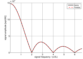
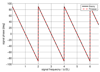
Figure 1: Plots showing the amplitude and phase of the upper sideband produced when a gravitational wave modulates a space of length $L=10$ km against the signal frequency of the gravitational wave. The signal frequency is normalised with respect to the of the light round-trip of space $L$, or the free-spectral-range of a cavity of length $L$.

4 Reflection from a mirror

We now consider the effect of a gravitational wave on a beam propagating through a space of length $L$ where it is then reflected from a mirror and propagates back through the space (see figure 2). Is this just equivalent to a space of double the length, taking into account the reflectivity of the mirror?

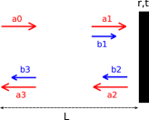
Figure 2: A diagram of a single reflection from a mirror. $a$ represent the carrier field, $b$ represent the upper and lower sidebands produced by a gravitational wave.

In this case the effect of the gravitational wave in calculated by considering the sidebands added at different points in the setup, after each length propagation. As the modulation index, $m$, is small we assume the carrier field amplitude is unchanged due to the gravitational wave. Referring to the fields in figure 2, where $a$ refers to the field of the carrier and $b$ refer to the field of the sidebands we have:

$$\begin{split}{}&a_{3}=a_{2}\exp{(-ik_{0}L)}\\ {}&a_{2}=ra_{1}\\ {}&a_{1}=a_{0}\exp{(-ik_{0}L)}\end{split}$$

So the reflected carrier field is given by:

$$a_{3}=ra_{0}\exp{(-i2k_{0}L)}$$ (18)

For the sideband fields we have:

$$\begin{split}{}&b_{3}=b_{2}\exp{(-i(k_{0}\pm k_{g})L)}+a_{2}\ \alpha_{sb}^{\mathrm{space}}\\ {}&b_{2}=rb_{1}\\ {}&b_{1}=a_{0}\ \alpha_{sb}^{\mathrm{space}}\\ \end{split}$$

where $\alpha_{sb}^{\mathrm{space}}$ describes the relative amplitude and phase of the sideband created from the modulation of the space. This gives the reflected field of the sidebands as:

$$\begin{split}b_{3}{}&=ra_{0}\ \alpha_{sb}^{\mathrm{space}}\exp{(-i(k_{0}\pm k_{g})L)}+ra_{0}\ \alpha_{sb}^{\mathrm{space}}\exp{(-ik_{0}L)}\\ {}&=ra_{0}\ \alpha_{sb}^{\mathrm{space}}\exp{(-ik_{0}L)}\left[1+\exp{(\mp ik_{g}L)}\right]\\ \end{split}$$ (19)

The sidebands produced from the round-trip propagation and single reflection have combined amplitude and phase $a_{0}\ \alpha_{sb}^{\mathrm{arm}}$ where:

$$\alpha_{sb}^{\mathrm{arm}}=r\alpha_{sb}^{\mathrm{space}}\exp{(-ik_{0}L)}[1+\exp{(\mp ik_{g}L)}]$$ (20)

and if we assume the space is ‘resonant’ for the carrier wave we can simplify this to:

$$\alpha_{sb}^{\mathrm{arm}}=r\alpha_{sb}^{\mathrm{space}}[1+\exp{(\mp ik_{g}L)}]$$ (21)

Figure 3 shows plots of the amplitude and phase of the upper sideband for propagation back-and-forth from a mirror ($L=10$ km, $r=1$), comparing these analytical equations and the result from Finesse. The Finesse output is generated by the following commands:

l l1 1 0 n1s s1 10k 1 n1 n2m m1 1 0 0 n2 n3fsig sm s1 1 0ad upper 1 n1xaxis sm f lin 1 50k 400put upper f $x1yaxis abs:degThe plots illustrate that this propagation back-and-forth is equivalent to the modulation of a space of double the length (the plots are identical to those shown in figure 1 except the $x$-axis is scaled by 2).

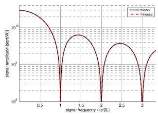
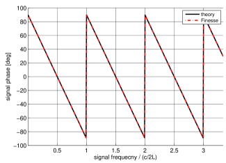
Figure 3: Plots showing the amplitude and phase of the upper sideband produced when a gravitational wave modulates a carrier field which propagates along a space of length $L=10$ km and is then reflected by a mirror ($r=1$) and travels the same $10$ km back again. This is the same result as shown in Figure 1 except for the fact that the $x$-axis is scaled by a factor of two (and in this plot the $y$-axis uses a log-scale).

5 Linear cavities

We now consider the sidebands reflected from a Fabry-Perot cavity when the cavity space is modulated by a gravitational wave. Figure 4 shows the different fields at different points in a linear cavity.

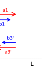
Figure 4: A diagram showing the carrier and sideband fields at different points in a linear cavity. $a$ represent the carrier field, $b$ represent the upper and lower sidebands produced by a gravitational wave.

The sideband field reflected from a linear cavity is:

$$b_{4}=it_{1}b_{3}^{\prime}$$ (22)

where

$$\begin{split}{}&b_{3}^{\prime}=a_{1}\alpha_{sb}^{\mathrm{arm}}+r_{2}b_{1}\exp{(-i2(k_{0}\pm k_{g})L)}\\ {}&b_{1}=r_{1}b_{3}^{\prime}\\ {}&b_{3}^{\prime}=\frac{a_{1}\alpha_{sb}^{\mathrm{arm}}}{1-r_{1}r_{2}\exp{(-i2(k_{0}\pm k_{g})L)}}\end{split}$$

and $\alpha_{sb}^{\mathrm{arm}}$ refers to the relative amplitude and phase of the sidebands after propagation back-and-forth from the end mirror. The carrier fields are solved by the usual simultaneous equations:

$$\begin{split}{}&a_{1}=it_{1}a_{0}+r_{1}a_{3}^{\prime}\\ {}&a_{3}^{\prime}=a_{3}\exp{(-ik_{0}L)}\\ {}&a_{3}=r_{2}a_{1}^{\prime}\\ {}&a_{1}^{\prime}=a_{1}\exp{(-ik_{0}L)}\end{split}$$

from which we have:

$$\begin{split}{}&a_{1}=it_{1}a_{0}+r_{1}r_{2}a_{1}\exp{(-i2k_{0}L)}\\ {}&a_{1}=\frac{it_{1}a_{0}}{1-r_{1}r_{2}\exp{(-i2k_{0}L)}}\end{split}$$ (23)

Finally:

$$\begin{split}b_{4}{}&=\frac{-T_{1}a_{0}}{1-r_{1}r_{2}\exp{(-i2k_{0}L)}}\frac{1}{1-r_{1}r_{2}\exp{(-i2(k_{0}\pm k_{g})L)}}\alpha_{sb}^{\mathrm{arm}}\end{split}$$ (24)

The sidebands reflected from a Fabry-Perot cavity are given by the field $a_{0}\ \alpha_{sb}^{\mathrm{FP}}$, where:

$$\alpha_{sb}^{\mathrm{FP}}=\frac{-T_{1}}{1-r_{1}r_{2}}\frac{\alpha_{sb}^{\mathrm{arm}}}{1-r_{1}r_{2}\exp{(\mp i2k_{g}L)}}$$ (25)

if we assume the cavity is on resonance. In figure 5 plots of this analytic result for a 10 km long cavity are compared with the result from Finesse. The Finesse output is generated with the following file:

l l1 1 0 nins s0 1 nin n1const T_ITM 700e-3const T_ETM 100e-6m1 ITM $T_ITM 0 0 n1 n2s sarm 10k n2 n3 m1 ETM $T_ETM 0 180 n3 n4fsig sig1 sarm 1 0ad upper 0 n1xaxis sig1 f lin 100 50k 400put upper f $x1yaxis lin abs:deg

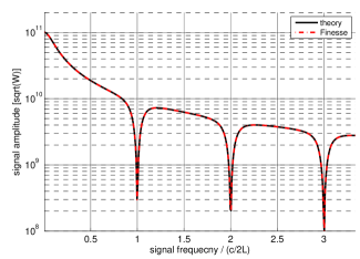
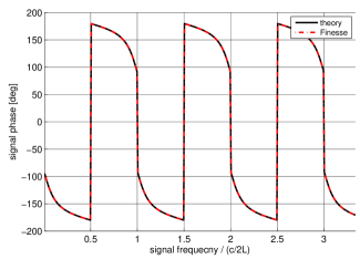
Figure 5: Plots showing the amplitude and phase of the upper sideband produced by a gravitational wave modulating a Fabry-Perot cavity of length $L=10$ km at frequency against the signal frequency. The sideband is detected in the light reflected from the cavity.

6 Michelson interferometer

We now look at the effect of a gravitational wave on the output of a Michelson interferometer. The amplitude of the sidebands at the output of the detector is given by:

$$b_{out}=r_{bs}b_{x}+i\ t_{bs}b_{y}$$ (26)

where $r_{bs}$ and $t_{bs}$ refer to the reflection and transmission coefficients of the beam-splitter and $b_{x}$ and $b_{y}$ are the sideband fields reflected from the $x$ and $y$ arms. If we consider a gravitational wave in the ideal polarisation for a Michelson (a gravitational wave, $h_{+}$, modulating the space in the $y$ arm 180^∘ out of phase with the $x$ arm) we have:

$$\begin{split}{}&b_{x}=i\ t_{bs}\ (a_{0}\exp{(-ik_{0}l_{x})})\ \alpha_{sb}^{\mathrm{FP}}\exp{(-i(k_{0}\pm k_{g})l_{x})}\\ {}&b_{y}=r_{bs}\ (a_{0}\exp{(-ik_{0}l_{y})})\ (-\alpha_{sb}^{\mathrm{FP}})\exp{(-i(k_{0}\pm k_{g})l_{y})}\end{split}$$

where $l_{x}$ and $l_{y}$ refer to the Michelson lengths, which should be much smaller than the cavity lengths. In order to operate on the dark fringe we must have $|l_{x}-l_{y}|=(2N+1)\frac{\lambda}{4}$, where $N$ is an integer. Finally, at the output of the interferometer we have:

$$b_{out}=i\ t_{bs}r_{bs}a_{0}\alpha_{sb}^{\mathrm{FP}}\left[\exp{(-i(2k_{0}\pm k_{g})l_{x})}-\exp{(-i(2k_{0}\pm k_{g})l_{y})}\right]$$ (27)

For the case of no arm cavities (i.e. just a single mirror at the end of the arm) just replace the $\alpha_{sb}^{\mathrm{FP}}$ factor with $\alpha_{sb}^{\mathrm{arm}}$. In figure 6 this analytic result and the result from a Finesse simulation of the same setup are plotted, for a simple Michelson and a Michelson with arm cavities. The Finesse output is generated using the following code:

For a simple Michelson without arm cavities:

l l1 1 0 nin

s s0 1 nin n1

const T_ETM 100e-6

bs BS 0.5 0.5 0 45 n1 ny1 nx1 nout

s syarm 10k ny1 ny2 ¯¯¯
m1 ETMy $T_ETM 0 0 ny2 ny3

s sxarm 10k nx1 nx2 ¯¯¯
m1 ETMx $T_ETM 0 90 nx2 nx3

fsig sig1 syarm 1 180
fsig sig1 sxarm 1 0

ad upper 0 nout

xaxis sig1 f lin 100 50k 400
put upper f $x1
yaxis lin abs:deg

For a Michelson with arm cavities:

l l1 1 0 nin

s s0 1 nin n1

const T_ITM 700e-3
const T_ETM 100e-6

bs BS 0.5 0.5 0 45 n1 ny1 nx1 nout

s sy 1 ny1 ny2

m1 ITMy $T_ITM 0 0 ny2 ny3
s syarm 10k ny3 ny4 ¯¯¯
m1 ETMy $T_ETM 0 0 ny4 ny5

s sx 1 nx1 nx2

m1 ITMx $T_ITM 0 90 nx2 nx3
s sxarm 10k nx3 nx4 ¯¯¯
m1 ETMx $T_ETM 0 90 nx4 nx5

fsig sig1 syarm 1 180
fsig sig1 sxarm 1 0

ad upper 0 nout

xaxis sig1 f lin 100 50k 400
put upper f $x1
yaxis lin abs:deg

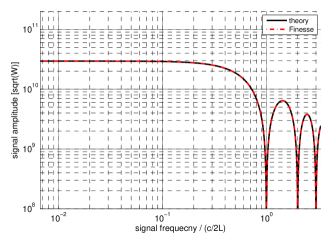
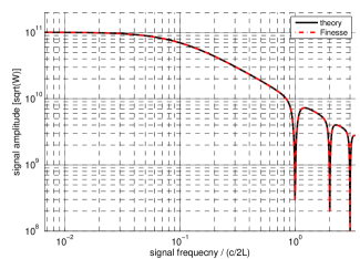
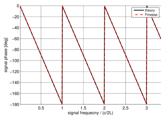
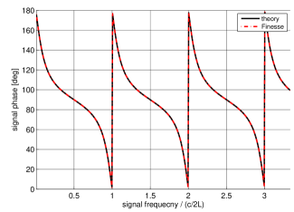
Figure 6: Plots showing the amplitude and phase of the upper sideband produced by a gravitational wave modulating the 10 km long arms of a Michelson interferometer. Left: Plots of the amplitude (top) and phase (bottom) of the sidebands at the output of a simple Michelson with no arm cavities. Right: Plots of the amplitude (top) and phase (bottom) of the sidebands at the output of a Michelson with Fabry-Perot arm cavities.

7 Sagnac

We now look at the gravitational wave effect on the output of a Sagnac interferometer. The sideband fields at the output of the detector are given by:

$$b_{\mathrm{out}}=it_{bs}b_{a}+r_{bs}b_{c}$$ (28)

$b_{c}$ and $b_{a}$ refer to the sidebands generated travelling clockwise and anti-clockwise through the interferometer. Travelling clockwise through the interferometer we have:

$$b_{c}=b_{c}^{x}+b_{c}^{y}R_{cav}(k_{0}\pm k_{g})$$ (29)

where $b_{c}^{x}$ and $b_{c}^{y}$ refer to the sidebands created in the $x$ and $y$ arms. $R_{cav}$ is the complex number describing the reflected field from a cavity:

$$R_{cav}(k)=r_{1}-\frac{T_{1}r_{2}\exp{(-2ikL)}}{1-r_{1}r_{2}\exp{(-2ikL)}}$$ (30)

If there is no arm cavity $T_{1}=1$ and $r_{1}=0$ and an additional $180^{\circ}$ needs to be added to $R_{cav}$ (mitigating the $90^{\circ}$ phase incurred for each transmission through the input mirror). The sidebands created travelling clockwise through the $y$ arm are given by:

$$b_{c}^{y}=r_{bs}a_{0}(-\alpha_{sb}^{\mathrm{FP}})$$ (31)

The minus refers to the relative phase of the modulation by the gravitational wave. The sidebands created travelling clockwise through the $x$ arm are given by:

$$b_{c}^{x}=r_{bs}a_{0}R_{cav}(k_{0})\alpha_{sb}^{\mathrm{FP}}$$ (32)

So we have:

$$b_{c}=r_{bs}\ a_{0}\ \alpha_{sb}^{\mathrm{FP}}\left[R_{cav}(k_{0})-R_{cav}(k_{0}\pm k_{g})\right]$$ (33)

The sidebands created travelling anti-clockwise through the interferometer are given by:

$$b_{a}=b_{a}^{x}R_{cav}(k_{0}\pm k_{g})+b_{a}^{y}$$ (34)

We have the sidebands created travelling anti-clockwsie through the $x$-arm:

$$b_{a}^{x}=it_{bs}\ a_{0}\ \alpha_{sb}^{\mathrm{arm}}$$ (35)

The sidebands created travelling anti-clockwise through the $y$-arm ($-\alpha_{sb}^{\mathrm{arm}}$ to take into account $h_{+}$ is out of phase by $\pi$ with respect to the $x$ arm):

$$b_{a}^{y}=it_{bs}a_{0}R_{cav}(k_{0})(-\alpha_{sb}^{\mathrm{arm}})$$ (36)

Which gives the total anti-clockwise sideband field as:

$$b_{a}=i\ t_{bs}\ a_{0}\ \alpha_{sb}^{\mathrm{FP}}\left[R_{cav}(k_{0}\pm k_{g})-R_{cav}(k_{0})\right]$$ (37)

Finally the sidebands at the output of the interferometer are given by:

$$\begin{split}b_{out}{}&=a_{0}\ \alpha_{sb}^{\mathrm{FP}}\left[R_{cav}(k_{0})-R_{cav}(k_{0}\pm k_{g})\right]\left[R_{bs}-i^{2}T_{bs}\right]\\ {}&=a_{0}\ \alpha_{sb}^{\mathrm{FP}}\left[R_{cav}(k_{0})-R_{cav}(k_{0}\pm k_{g})\right]\left[R_{bs}+T_{bs}\right]\end{split}$$ (38)

In figure 7 this analytical solution is plotted, as well as the result for a Finesse simulation, for a simple Sagnac and a Sagnac with arm cavities. The Finesse simulation is detailed in the following kat files:

For a simple Sagnac without arm cavities:

 l1 1 0 nin

s s0 1 nin n1

const T_ETM 100e-6

bs BS 0.5 0.5 0 45 n1 ny1 nx1 nout

s syarm1 10k ny1 ny2 ¯¯¯
bs1 ETMy $T_ETM 0 0 0 ny2 ny3 nytrans dump1
s syarm2 10k ny3 ny4

bs TM 1 0 0 45 ny4 nx4 dump2 dump3

s sxarm1 10k nx1 nx2 ¯¯¯
bs1 ETMx $T_ETM 0 0 0 nx2 nx3 nxtrans dump4
s sxarm2 10k nx3 nx4

fsig sig1 syarm1 1 180
fsig sig1 syarm2 1 180
fsig sig1 sxarm1 1 0
fsig sig1 sxarm2 1 0

ad upper 0 nout

xaxis sig1 f lin 100 50k 400
put upper f $x1
yaxis lin abs:deg

For a Sagnac with arm cavities:

l l1 1 0 nin

s s0 1 nin n1

const T_ITM 700e-3
const T_ETM 100e-6

bs BS 0.5 0.5 0 45 n1 ny1 nx1 nout

s sy 1 ny1 ny2

bs1 ITMy $T_ITM 0 0 0 ny2 ny3 ny4 ny5
s syarm1 10k ny4 ny6 ¯¯¯
bs1 ETMy $T_ETM 0 0 0 ny6 ny7 ny8 dump1
s syarm2 10k ny7 ny5

bs TM 1 0 0 45 ny3 nx3 dump2 dump3

s sx 1 nx1 nx2

bs1 ITMx $T_ITM 0 0 0 nx2 nx3 nx4 nx5
s sxarm1 10k nx4 nx6 ¯¯¯
bs1 ETMx $T_ETM 0 0 0 nx6 nx7 nx8 dump4
s sxarm2 10k nx7 nx5

fsig sig1 syarm1 1 180
fsig sig1 syarm2 1 180
fsig sig1 sxarm1 1 0
fsig sig1 sxarm2 1 0

ad upper 0 nout

xaxis sig1 f lin 100 50k 400
put upper f $x1
yaxis lin abs:deg

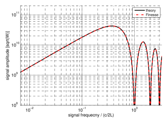
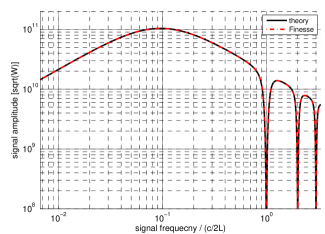
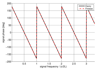
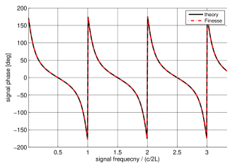
Figure 7: Plots showing the amplitude and phase of the upper sideband produced by a gravitational wave modulating the arms of a Sagnac interferometer. Left: Plots of the amplitude (top) and phase (bottom) of the sidebands at the output of a simple Sagnac with no arm cavities. Right: Plots of the amplitude (top) and phase (bottom) of the sidebands at the output of a Sagnac with Fabry-Perot arm cavities. The arms in both cases have length $L=$10 km.

References

• [1] A. Freise, G. Heinzel, H. Lück, R. Schilling, B. Willke, and K. Danzmann, “Frequency-domain interferometer simulation with higher-order spatial modes,” Class. Quantum Grav. 21, S1067 (2004), the program is available at http://www.gwoptics.org/finesse
• [2] J. Mizuno, Comparison of optical configurations for laser-interferometric gravitational-wave detectors, PhD. Thesis, University of Hannover (1995).