Semiparametric Gaussian copula models: Geometry and efficient rank-based estimation

Abstract

We propose, for multivariate Gaussian copula models with unknown margins and structured correlation matrices, a rank-based, semiparametrically efficient estimator for the Euclidean copula parameter. This estimator is defined as a one-step update of a rank-based pilot estimator in the direction of the efficient influence function, which is calculated explicitly. Moreover, finite-dimensional algebraic conditions are given that completely characterize efficiency of the pseudo-likelihood estimator and adaptivity of the model with respect to the unknown marginal distributions. For correlation matrices structured according to a factor model, the pseudo-likelihood estimator turns out to be semiparametrically efficient. On the other hand, for Toeplitz correlation matrices, the asymptotic relative efficiency of the pseudo-likelihood estimator can be as low as 20%. These findings are confirmed by Monte Carlo simulations. We indicate how our results can be extended to joint regression models.

FLA

, and t4Supported by contract “Projet d’Actions de Recherche Concertées” No. 12/17-045 of the “Communauté française de Belgique” and by IAP research network Grant nr. P7/06 of the Belgian government (Belgian Science Policy).

1 Introduction

Let $\mathbf{X}=(X_{1},\ldots,X_{p})^{\prime}$ be a $p$-dimensional random vector with absolutely continuous marginal distribution functions $F_{1},\ldots,F_{p}$ and joint distribution function $F$. The copula, $C$, of $F$ is the joint distribution function of the vector $\mathbf{U}=(U_{1},\ldots,U_{p})^{\prime}$ with $U_{j}=F_{j}(X_{j})$, uniformly distributed on $(0,1)$. By Sklar’s theorem,

$$F(\mathbf{x})=C\bigl{(}F_{1}(x_{1}),\ldots,F_{p}(x_{p})\bigr{)},\qquad\mathbf{x}\in\mathbb{R}^{p},$$

yielding a separation of $F$ into its margins $F_{1},\ldots,F_{p}$ and its copula $C$. The copula remains unchanged if strictly increasing transformations are applied to the $p$ components of $\mathbf{X}$.

A semiparametric copula model for the law of the random vector $\mathbf{X}$ is a model where $F$ is allowed to have arbitrary, absolutely continuous margins and a copula $C_{\theta}$ which belongs to a finite-dimensional parametric family. An important inference problem is the development of an efficient estimator of the copula parameter $\theta$ on the basis of a random sample $\mathbf{X}_{i}=(X_{i1},\ldots,X_{ip})^{\prime}$, $i=1,\ldots,n$. The marginal distributions $F_{1},\ldots,F_{p}$ are thus considered as infinite-dimensional nuisance parameters. In accordance to the structure of the model, a desirable property for the estimator of $\theta$ is that it is invariant with respect to strictly increasing transformations applied to the $p$ components. This is equivalent to the requirement that the estimator is measurable with respect to the vectors of ranks, $\mathbf{R}_{i}^{(n)}=(R_{i1}^{(n)},\ldots,R_{ip}^{(n)})^{\prime}$, with $R_{ij}^{(n)}$ the rank of $X_{ij}$ within the $j$th marginal sample $X_{1j},\ldots,X_{nj}$; see also Hoff [(2007), Section 5], who shows that the ranks are G-sufficient.

There exist a number of rank-based estimation strategies for $\theta$, none of them guaranteed to be semiparametrically efficient. The most common are method-of-moment type estimators [Oakes (1986), Genest and Rivest (1993), Klüppelberg and Kuhn (2009), Brahimi and Necir (2012), Liu et al. (2012)], minimum-distance estimators [Tsukahara (2005), Liebscher (2009)], and the pseudo-likelihood estimator [Oakes (1994), Genest, Ghoudi and Rivest (1995)]. For vine copulas, the pseudo-likelihood estimator and variants thereof are studied in Hobæk Haff (2013). An expectation–maximization algorithm for a Gaussian copula mixture model is proposed in Li et al. (2011).

Conditions for the efficiency of the pseudo-likelihood estimator are derived in Genest and Werker (2002), where it is concluded that efficiency is the exception rather than the rule. One notable exception is the bivariate Gaussian copula model (see below), where the pseudo-likelihood estimator is asymptotically equivalent to the normal scores rank correlation coefficient, shown to be efficient in Klaassen and Wellner (1997).

A semiparametrically efficient estimator for the copula parameter is proposed in Chen, Fan and Tsyrennikov (2006). However, the estimator is based on parametric sieves for the unknown margins, so that the estimator is not invariant under increasing transformations of the component variables, that is, the estimator is not rank-based. Moreover, it requires the choice of the orders of the sieves as tuning parameters. The approach has been extended to Markov processes [Chen, Wu and Yi (2009)] and to bivariate survival data [Cheng et al. (2014)].

Besides the already mentioned paper by Klaassen and Wellner (1997), the issue of efficient, rank-based estimation is taken up in Hoff, Niu and Wellner (2014) for the important class of semiparametric Gaussian copula models with structured correlation matrices. They derive the semiparametric lower bound to the asymptotic variance of rank-based regular estimators for the copula parameter. However, they do not provide such an estimator. They also construct a specific Gaussian copula model for which the pseudo-likelihood estimator is not efficient. They conclude their paper with the suggestion that the maximum rank-likelihood estimator in Hoff (2007) may be efficient.

Following Klaassen and Wellner (1997) and Hoff, Niu and Wellner (2014), we put the focus in this paper on semiparametric Gaussian copula models. In the context of graphical models for high-dimensional random vectors, these have been called “nonparanormal” models, that is, the variables follow a joint normal distribution after a set of unknown monotone transformations [Liu et al. (2012), Xue and Zou (2012)]. Allowing for covariates, semiparametric Gaussian copula models also lead to semiparametric regression models [Song (2000), Song, Li and Yuan (2009), Basrak and Klaassen (2013)].

The Gaussian copula $C_{\theta}$ is the copula of a $p$-variate Gaussian distribution $N_{p}(0,R(\theta))$ with $p\times p$ positive definite correlation matrix $R(\theta)$:

$$\qquad C_{\theta}(\mathbf{u})=\Phi_{\theta}\bigl{(}\Phi^{-1}(u_{1}),\ldots,\Phi^{-1}(u_{p})\bigr{)},\qquad\mathbf{u}=(u_{1},\ldots,u_{p})\in(0,1)^{p},$$ (1)

with $\Phi_{\theta}$ the $N_{p}(0,R(\theta))$ cumulative distribution function and $\Phi^{-1}$ the standard normal quantile function. In the unrestricted Gaussian copula model, $R(\theta)$ can be any $p\times p$ positive definite correlation matrix. Submodels arise by considering structured correlation matrices. In that case, the dimension, $k$, of the parameter set is smaller than the number of pairs of variables, $p(p-1)/2$. As model for one observation, we thus consider

$$\mathcal{P}=(\mathrm{P}_{\theta,F_{1},\ldots,F_{p}}|\theta\in\Theta,F_{1},\ldots,F_{p}\in\mathcal{F}_{\mathrm{ac}}),\qquad\Theta\subset\mathbb{R}^{k},$$ (2)

where $\mathcal{F}_{\mathrm{ac}}$ denotes the set of absolutely continuous distributions on the real line and $\mathrm{P}_{\theta,F_{1},\ldots,F_{p}}$ denotes the law of the random vector $\mathbf{X}$ which has copula (1) and margins $F_{1},\ldots,F_{p}$.

For the model $\mathcal{P}$, we compute the efficient score and influence functions and the efficient information matrix for $\theta$. The computations are based on a detailed analysis of the tangent space structure of the model. The practical interest of this analysis is that it yields an efficient semiparametric, rank-based estimator for $\theta$. Starting from an initial, rank-based, $\sqrt{n}$-consistent estimator, our estimator is defined as a one-step update in the direction of the estimated efficient influence function. The idea of constructing an efficient estimator via a one-step update is already to be found in Bickel [(1982), Remark 1], who refers in turn to Le Cam [(1969), Theorem 4].

Existence of an initial estimator is usually no problem: take the pseudo-likelihood estimator, use a minimum-distance estimator, or express the parameter components as functions of the entries of the correlation matrix and use a plug-in estimator based on the normal scores correlation coefficients. In the semiparametric Gaussian copula model, the update step is easy to implement, relying on simple matrix algebra.

We thereby provide a positive answer to the conjecture formulated in Hoff, Niu and Wellner (2014) whether it is possible to attain the semiparametric lower bound using a rank-based estimator. We wish to stress the fact that, in contrast to the sieve-based estimator in Chen, Fan and Tsyrennikov (2006), our estimator is rank-based, and thus invariant with respect to increasing transformations of the component variables, in accordance with the group structure of the model. Note, however, that the methodology in Chen, Fan and Tsyrennikov (2006) also applies to general, not necessarily Gaussian, copula models.

By restricting attention to estimators with influence functions of a certain form, we construct an algebraic framework which allows for particularly simple, finite-dimensional conditions on the parametrization $\theta\mapsto R(\theta)$ for efficiency of the pseudo-likelihood estimator and for adaptivity of the model. These are detailed for a large number of examples. The pseudo-likelihood estimator turns out to be efficient not only in the unrestricted model, confirming a remark in Klaassen and Wellner (1997), but also in the often-used class of factor models. On the other hand, for correlation matrices with a Toeplitz structure, the pseudo-likelihood estimator can be quite inefficient, with an asymptotic relative efficiency as low as 20%. Although Hoff, Niu and Wellner (2014) already identified a Gaussian copula model for which the pseudo-likelihood estimator is inefficient, the asymptotic relative efficiency of the pseudo-likelihood estimator in their example was still not far from 100%. The asymptotic results are complemented by a Monte Carlo study, confirming the above theoretical findings for small samples, even in high dimensions.

The outline of the paper is as follows. In Section 2, we study the model’s tangent space, culminating in the calculation of the efficient score function and information matrix for $\theta$. These serve to define the one-step estimator in Section 3, where its semiparametric efficiency is proved. Simple criteria for efficiency of estimators and of adaptivity of the model are established in Section 4. Examples and numerical illustrations are provided in Section 5. Section 6 concludes and discusses extensions to other copula families and to joint regression models. Detailed proofs are deferred to the Appendices, which are collected in the supplement [Segers, van den Akker and Werker (2014)].

2 Tangent space and efficient score

The purpose of this section is to compute the semiparametric lower bound for estimating the Gaussian copula parameter $\theta$. Main keys to obtain this lower bound are the tangent space of the semiparametric Gaussian copula model $\mathcal{P}$ and the efficient score function for $\theta$; see Bickel et al. [(1993), Chapters 2–3] and van der Vaart [(2000), Chapter 25] for detailed expositions on these notions. Readers mainly interested in our rank-based efficient estimator for $\theta$ may want to jump to Section 3 on a first reading.

Section 2.1 states our assumptions and introduces notation that will be used throughout. Section 2.2 shortly discusses the Gaussian copula model with known marginals. In Sections 2.3 and 2.4, we determine the tangent space and efficient score function, respectively. The tangent space theory in Section 2.3 is inspired upon the one for bivariate semiparametric copula models in Bickel et al. [(1993), Section 4.7].

2.1 Assumptions and notation

The log density of the Gaussian copula (1) with $p\times p$ correlation matrix $R(\theta)$ is given by

$$\ell(\mathbf{u};\theta)=\log c_{\theta}(\mathbf{u})=-\tfrac{1}{2}\log\bigl{(}\det R(\theta)\bigr{)}-\tfrac{1}{2}\mathbf{z}^{\prime}\bigl{(}R^{-1}(\theta)-I_{p}\bigr{)}\mathbf{z},$$ (3)

for $\mathbf{u}\in(0,1)^{p}$, where $I_{p}$ is the $p\times p$ identity matrix and where $\mathbf{z}=(z_{1},\ldots,z_{p})^{\prime}$ with $z_{j}=\Phi^{-1}(u_{j})$. Nonsingularity of the correlation matrix is part of the following assumption.

Assumption 2.1.

Suppose $\Theta\subset\mathbb{R}^{k}$ is open and: [(iii)]

the mapping $\theta\mapsto R(\theta)$ is one-to-one;

for all $\theta\in\Theta$, the inverse $S(\theta)=R^{-1}(\theta)$ exists;

for all $\theta\in\Theta$, the matrices of partial derivatives $\dot{R}_{1}(\theta),\ldots,\dot{R}_{k}(\theta)$, defined by $\dot{R}_{m,ij}(\theta)=\partial R_{ij}(\theta)/\partial\theta_{m}$, for $m=1,\ldots,k$ and $i,j=1,\ldots,p$, exist and are continuous in $\theta$;

for all $\theta\in\Theta$, the matrices $\dot{R}_{1}(\theta),\ldots,\dot{R}_{k}(\theta)$ are linearly independent.

Let us also define $p\times p$ matrices $\dot{S}_{m}(\theta)$ by $\dot{S}_{m,ij}(\theta)=\partial S_{ij}(\theta)/\partial\theta_{m}$. These derivatives satisfy $\dot{S}_{m}(\theta)=-S(\theta)\dot{R}_{m}(\theta)S(\theta)$, which follows from differentiating $R(\theta)S(\theta)=I_{p}$ [Magnus and Neudecker (1999), Section 8.4].

The $p$-dimensional vector $\mathbf{X}=(X_{1},\ldots,X_{p})^{\prime}$ denotes, as in the Introduction, a random vector with copula (1) and margins $F_{1},\ldots,F_{p}\in\mathcal{F}_{\mathrm{ac}}$. Its law is denoted by $\mathrm{P}_{\theta,F_{1},\ldots,F_{p}}$ and expectations with respect to this law are denoted by $\mathrm{E}_{\theta,F_{1},\ldots,F_{p}}$. In case all margins are uniform on $[0,1]$, notation $\operatorname{Un}[0,1]$, we use $\mathbf{U}$, $\mathrm{P}_{\theta}$ and $\mathrm{E}_{\theta}$ as notation. Let $\mathbf{Z}=(Z_{1},\ldots,Z_{p})^{\prime}$ be defined by $Z_{j}=\Phi^{-1}(U_{j})$ and note that $\mathbf{Z}\sim\Phi_{\theta}$ under $\mathrm{P}_{\theta}$.

Moreover, we consider a measurable space $(\Omega,\mathcal{F})$ supporting probability measures $\mathbb{P}_{\theta,F_{1},\ldots,F_{p}}$, for $\theta\in\Theta$ and $F_{1},\ldots,F_{p}\in\mathcal{F}_{\mathrm{ac}}$, and i.i.d. random vectors $\mathbf{X}_{i}$, $i\in\mathbb{N}$, each with law $\mathrm{P}_{\theta,F_{1},\ldots,F_{p}}$ under $\mathbb{P}_{\theta,F_{1},\ldots,F_{p}}$. Expectations with respect to $\mathbb{P}_{\theta,F_{1},\ldots,F_{p}}$ are denoted by $\mathbb{E}_{\theta,F_{1},\ldots,F_{p}}$. Furthermore, $\mathbb{P}_{\theta}$ is shorthand for $\mathbb{P}_{\theta,\operatorname{Un}[0,1],\ldots,\operatorname{Un}[0,1]}$, for which expectations are denoted by $\mathbb{E}_{\theta}$.

2.2 The Gaussian copula model with known margins

The starting point of the analysis is the case that the margins $F_{1},\ldots,F_{p}\in\mathcal{F}_{\mathrm{ac}}$ are known. In particular, we compute the Fisher information matrix for $\theta$ in this case. Due to the transformation structure of the model, it suffices to consider uniform margins, that is, to consider the model $\mathcal{P}_{\mathrm{km}}=(\mathrm{P}_{\theta}|\theta\in\Theta)$.

Under Assumption 2.1, the score $\dot{\ell}_{\theta}(\mathbf{u};\theta)=(\dot{\ell}_{\theta,m}(\mathbf{u};\theta))_{m=1}^{k}$ is given by

$$\dot{\ell}_{\theta,m}(\mathbf{u};\theta)=\frac{\partial}{\partial\theta_{m}}\ell(\mathbf{u};\theta)=-\frac{1}{2}\operatorname{tr}\bigl{(}S(\theta)\dot{R}_{m}(\theta)\bigr{)}-\frac{1}{2}\mathbf{z}^{\prime}\dot{S}_{m}(\theta)\mathbf{z},$$ (4)

for $\mathbf{u}\in(0,1)^{p}$, where the partial derivative of $\det R(\theta)$ follows from Jacobi’s formula [Magnus and Neudecker (1999), Section 8.3]. The $k\times k$ Fisher information matrix is defined by $I(\theta)=\mathrm{E}_{\theta}[\dot{\ell}_{\theta}\dot{\ell}_{\theta}^{\prime}(\mathbf{U};\theta)]$.

To obtain a convenient representation of $I(\theta)$, we introduce an inner product on the linear space $\operatorname{Sym}(p)$ of real symmetric $p\times p$ matrices. For $A,B\in\operatorname{Sym}(p)$, put

$$\langle{A},{B}\rangle_{\theta}=\operatorname{cov}_{\theta}\bigl{(}\tfrac{1}2\mathbf{Z}^{\prime}A\mathbf{Z},\tfrac{1}2\mathbf{Z}^{\prime}B\mathbf{Z}\bigr{)}=\tfrac{1}2\operatorname{tr}\bigl{(}AR(\theta)BR(\theta)\bigr{)},$$ (5)

the covariance being calculated for $\mathbf{Z}\sim\Phi_{\theta}$. The latter equality follows from Theorem 12.10.12 in Magnus and Neudecker (1999). It is easily verified that $\langle{\cdot},{\cdot}\rangle_{\theta}$ defines an inner product on $\operatorname{Sym}(p)$. In particular, if $A\in\operatorname{Sym}(p)$ is such that $\langle{A},{A}\rangle_{\theta}=0$, then $\mathbf{Z}^{\prime}A\mathbf{Z}$ is almost surely equal to a constant and thus, $R(\theta)$ being nonsingular (Assumption 2.1), $A=0$.

From (4) and (5), we obtain, for $m,m^{\prime}=1,\ldots,k$,

$$I_{mm^{\prime}}(\theta)=\bigl{\langle}{-\dot{S}_{m}(\theta)},{-\dot{S}_{m^{\prime}}(\theta)}\bigr{\rangle}_{\theta},$$ (6)

which is continuous in $\theta$. Note that $I(\theta)$ is the Gram matrix associated to the matrices $-\dot{S}_{1}(\theta),\ldots,-\dot{S}_{k}(\theta)$, using (5) as inner product. Since Assumption 2.1 implies linear independence of $-\dot{S}_{1}(\theta),\ldots,-\dot{S}_{k}(\theta)$ (see part A of the proof of Proposition 2.8 below), the information matrix $I(\theta)$ is nonsingular.

From these observations, it follows that the Gaussian copula model with known margins is regular [Bickel et al. (1993), Definition 2.1.1 and Proposition 2.1.1]. For ease of reference, we state this fact in the following lemma.

Lemma 2.2

If the parametrization $\theta\mapsto R(\theta)$ satisfies Assumption 2.1, then the parametric Gaussian copula model with known, uniform margins is regular.

Remark 2.3.

Regularity of $\mathcal{P}_{\mathrm{km}}$ has some useful consequences: [(ii)]

The score function has zero expectation, $\mathrm{E}_{\theta}[\dot{\ell}_{\theta}(\mathbf{U};\theta)]=0$. This can also be seen from (4) and $\mathrm{E}_{\theta}(\mathbf{Z}^{\prime}A\mathbf{Z})=\operatorname{tr}(AR(\theta))$.

By the Hájek–Le Cam convolution theorem, the inverse of the Fisher information matrix, $I^{-1}(\theta)$, constitutes a lower bound to the asymptotic variance of regular estimators of $\theta$ in the model $\mathcal{P}_{\mathrm{km}}$ [see, e.g., van der Vaart (2000), Chapter 8].

2.3 Tangent space

In this section, we derive the tangent space of the semiparametric Gaussian copula model $\mathcal{P}$. The structure of the space is similar to the one of the bivariate semiparametric Gaussian copula model in Klaassen and Wellner (1997). In Section 2.4, we use this tangent space to calculate the efficient score for the copula parameter $\theta$. In turn, the efficient score determines the semiparametric lower bound for the asymptotic variance of regular estimators of $\theta$.

Informally, the tangent space at $\mathrm{P}_{\theta,F_{1},\ldots,F_{p}}\in\mathcal{P}$ is given by the collection of score functions of parametric submodels of $\mathcal{P}$. Such score functions can be thought of as functions on $\mathbb{R}^{p}$ of the form

$$\mathbf{x}\mapsto\frac{\partial}{\partial\eta}\log p_{\theta+\eta\alpha,F_{1,\eta},\ldots,F_{p,\eta}}(\mathbf{x})\bigg{|}_{\eta=0}.$$ (7)

Here, $\alpha\in\mathbb{R}^{k}$, while $p_{\theta+\eta\alpha,F_{1,\eta},\ldots,F_{p,\eta}}$ is the density of $\mathrm{P}_{\theta+\eta\alpha,F_{1,\eta},\ldots,F_{p,\eta}}\in\mathcal{P}$, depending on a real parameter $\eta$ taking values in a neighborhood of $0$. The marginal distributions are parametrized through paths $\eta\mapsto F_{j,\eta}$ in $\mathcal{F}_{\mathrm{ac}}$ that pass through $F_{j}$ at $\eta=0$.

The tangent space falls apart into two subspaces:

• a parametric part, arising from score functions of parametric submodels for which the margins are constant, $F_{j,\eta}=F_{j}$;

• a nonparametric part, arising from score functions of parametric submodels for which the copula parameter is constant, $\alpha=0$.

The parametric part corresponds in fact to the linear span of the score functions in the parametric Gaussian copula model with known margins. The nonparametric part describes the additional part of the model stemming from the margins being unknown.

Formally, the tangent space is a subspace of $\mathrm{L}_{2}(\mathrm{P}_{\theta,F_{1},\ldots,F_{p}})$, the space of square-integrable functions with respect to $\mathrm{P}_{\theta,F_{1},\ldots,F_{p}}$. The pointwise derivatives (7) will be replaced by derivatives in quadratic mean. The nonparametric part of the tangent space is described most conveniently as the image of a bounded linear operator, called score operator. It is the description and the analysis of this score operator that constitutes the gist of this section.

The density of $\mathrm{P}_{\theta,F_{1},\ldots,F_{p}}\in\mathcal{P}$ is given by

$$p_{\theta,F_{1},\ldots,F_{p}}(\mathbf{x})=c_{\theta}\bigl{(}F_{1}(x_{1}),\ldots,F_{p}(x_{p})\bigr{)}\prod_{j=1}^{p}f_{j}(x_{j}),\qquad\mathbf{x}\in\mathbb{R}^{p},$$

with $f_{1},\ldots,f_{p}$ the densities of $F_{1},\ldots,F_{p}$, respectively. If $\eta\mapsto F_{j,\eta}(x_{j})$ is differentiable at $\eta=0$, we obtain

$$\frac{\partial}{\partial\eta}\log p_{\theta,F_{1,\eta},\ldots,F_{p,\eta}}(\mathbf{x})\bigg{|}_{\eta=0}$$

$$\qquad=\sum_{j=1}^{p}\biggl{\{}\frac{\partial}{\partial\eta}\log f_{j,\eta}(x_{j})\bigg{|}_{\eta=0}+\dot{\ell}_{j}\bigl{(}F_{1}(x_{1}),\ldots,F_{p}(x_{p});\theta\bigr{)}\frac{\partial}{\partial\eta}F_{j,\eta}(x_{j})\bigg{|}_{\eta=0}\biggr{\}},$$

with, for $j=1,\ldots,p$ and $\mathbf{u}\in(0,1)^{p}$,

$$\dot{\ell}_{j}(\mathbf{u};\theta)=\frac{\partial}{\partial u_{j}}\ell(\mathbf{u};\theta)=\frac{z_{j}}{\varphi(z_{j})}-\sum_{i=1}^{p}S_{ij}(\theta)\frac{z_{i}}{\varphi(z_{j})},$$ (8)

where $\varphi$ denotes the standard normal density. Note that, for $u_{j}\in(0,1)$,

$$\mathrm{E}_{\theta}\bigl{[}\dot{\ell}_{j}(\mathbf{U};\theta)|U_{j}=u_{j}\bigr{]}=\frac{z_{j}}{\varphi(z_{j})}\Biggl{(}1-\sum_{i=1}^{p}S_{ij}(\theta)R_{ij}(\theta)\Biggr{)}=0.$$ (9)

The above formulas motivate the introduction of the following linear operators, which together will constitute the above mentioned score operator. Let $\mathrm{L}_{2}^{0}[0,1]$ be the subspace of $\mathrm{L}_{2}[0,1]=\mathrm{L}_{2}([0,1],\mathcal{B}_{[0,1]},\mathrm{d}\lambda)$ resulting from the restriction $\int h(\lambda)\,\mathrm{d}\lambda=0$ for $h\in\mathrm{L}_{2}[0,1]$. For $j=1,\ldots,p$, we introduce linear operators $\mathcal{O}_{\theta,j}:\mathrm{L}_{2}^{0}[0,1]\to\mathrm{L}_{2}(\mathrm{P}_{\theta})$ by

$$\mathcal{O}_{\theta,j}h=[\mathcal{O}_{\theta,j}h](\mathbf{U})=h(U_{j})+\dot{\ell}_{j}(\mathbf{U};\theta)H(U_{j}),$$ (10)

where $H(u)=\int_{0}^{u}h(\lambda)\,\mathrm{d}\lambda$ and where $\mathbf{U}$ is the identity mapping on $(0,1)^{p}$. The claim that the random variable on the right-hand side has a finite variance for $\mathbf{U}\sim\mathrm{P}_{\theta}$ is part of Lemma 2.4.

The score operator itself, $\mathcal{O}_{\theta}$, has domain $(\mathrm{L}_{2}^{0}[0,1])^{p}$ and is defined by

$$\mathcal{O}_{\theta}\mathbf{h}=\sum_{j=1}^{p}\mathcal{O}_{\theta,j}h_{j},\qquad\mathbf{h}=(h_{1},\ldots,h_{p})\in\bigl{(}\mathrm{L}_{2}^{0}[0,1]\bigr{)}^{p}.$$

Lemma 2.4 will present basic properties of $\mathcal{O}_{\theta,j}$ and $\mathcal{O}_{\theta}$. A formal description of the tangent space via the score operator will be given in Proposition 2.6.

To this end, we first need to introduce some additional notation. For $i,j=1,\ldots,p$ and $\mathbf{u}\in(0,1)^{p}$, we define

$$\ddot{\ell}_{ij}(\mathbf{u};\theta) = \frac{\partial}{\partial u_{i}}\dot{\ell}_{j}(\mathbf{u};\theta)$$

$$= \cases{\displaystyle\frac{z_{j}^{2}+1-S_{jj}(\theta)}{\varphi^{2}(z_{j})}-\sum_{t=1}^{p}S_{tj}(\theta)\frac{z_{t}z_{j}}{\varphi^{2}(z_{j})},&\quad$\mbox{if $i=j$;}$\vspace*{2pt}\cr\displaystyle-\frac{S_{ij}(\theta)}{\varphi(z_{i})\varphi(z_{j})},&\quad$\mbox{if $i\neq j$.}$}$$

For $u_{j}\in(0,1)$, we have

$$I_{jj}(u_{j};\theta) = \mathrm{E}_{\theta}\bigl{[}\dot{\ell}_{j}^{2}(\mathbf{U};\theta)|U_{j}=u_{j}\bigr{]}$$

$$= -\mathrm{E}_{\theta}\bigl{[}\ddot{\ell}_{jj}(\mathbf{U};\theta)|U_{j}=u_{j}\bigr{]}=\frac{S_{jj}(\theta)-1}{\varphi^{2}(z_{j})}.$$

From well-known results on Mill’s ratio [Gordon (1941)], we obtain the bound $1/\varphi(z_{j})\leq M\{u_{j}(1-u_{j})\}^{-1}$, for all $u_{j}\in(0,1)$ and some constant $M>0$. Hence, under Assumption 2.1, there exists a constant $M_{\theta}>0$ such that

$$I_{jj}(u_{j};\theta)\leq\frac{M_{\theta}}{\{u_{j}(1-u_{j})\}^{2}},\qquad u_{j}\in(0,1).$$ (12)

This bound is exploited in the proof of the following lemma, which states that $\mathcal{O}_{\theta}$ is a continuously invertible operator from $(\mathrm{L}_{2}^{0}[0,1])^{p}$ into $\mathrm{L}_{2}^{0}(\mathrm{P}_{\theta})$. Here we equip $(\mathrm{L}_{2}^{0}[0,1])^{p}$ with the inner product $\langle\mathbf{g},\mathbf{h}\rangle=\sum_{j=1}^{p}\int_{0}^{1}g_{j}(\lambda)h_{j}(\lambda)\,\mathrm{d}\lambda$ for $\mathbf{g},\mathbf{h}\in(\mathrm{L}_{2}^{0}[0,1])^{p}$, while $\mathrm{L}_{2}^{0}(\mathrm{P}_{\theta})$ is the subspace of $\mathrm{L}_{2}(\mathrm{P}_{\theta})$ resulting from the restriction $\mathrm{E}_{\theta}[f(\mathbf{U})]=0$ for $f\in\mathrm{L}_{2}(\mathrm{P}_{\theta})$.

Lemma 2.4

Let $\theta\mapsto R(\theta)$ be a parametrization that satisfies Assumption 2.1 and let $\theta\in\Theta$: [(a)]

The map $\mathcal{O}_{\theta,j}$, $j=1,\ldots,p$, is a bounded operator from $\mathrm{L}_{2}^{0}[0,1]$ into $\mathrm{L}_{2}^{0}(\mathrm{P}_{\theta})$. The map $\mathcal{O}_{\theta}$ is a bounded operator from $(\mathrm{L}_{2}^{0}[0,1])^{p}$ into $\mathrm{L}_{2}^{0}(\mathrm{P}_{\theta})$.

The operator $\mathcal{O}_{\theta}$ is continuously invertible on its range, $\mathrm{R}\mathcal{O}_{\theta}$, with inverse $\mathcal{O}_{\theta}^{-1}\dvtx\mathrm{L}_{2}^{0}(\mathrm{P}_{\theta})\to(\mathrm{L}_{2}^{0}[0,1])^{p}$ given by

$$\bigl{[}\mathcal{O}_{\theta}^{-1}f\bigr{]}_{j}(u_{j})=\mathrm{E}_{\theta}\bigl{[}f(\mathbf{U})|U_{j}=u_{j}\bigr{]},\qquad u_{j}\in(0,1),j=1,\ldots,p.$$

The proof is given in Appendix Ain the supplement. Here, we just note that the proof of part (a) follows the one of Proposition 4.7.2 in Bickel et al. (1993).

Remark 2.5.

An application of Banach’s theorem [see, e.g., Bickel et al. (1993), Proposition A.1.7] implies that $\mathrm{R}\mathcal{O}_{\theta}$ is closed.

We proceed with the construction of the tangent space. First, we define the “local paths” through $\mathcal{F}_{\mathrm{ac}}$. To this end, fix $F_{1},\ldots,F_{p}\in\mathcal{F}_{\mathrm{ac}}$ with densities $f_{1},\ldots,f_{p}$. Let $h_{1},\ldots,h_{p}\in\mathrm{L}^{0}_{2}[0,1]$ and introduce univariate densities $f_{j,\eta}(\cdot;h_{j})$, for $\eta\in(-1,1)$ and $j=1,\ldots,p$, by

$$f_{j,\eta}(x;h_{j})=d(\eta;f_{j},h_{j})g\bigl{(}\eta h_{j}\bigl{(}F_{j}(x)\bigr{)}\bigr{)}f_{j}(x),\qquad x\in\mathbb{R},$$

where $g(z)=2/(1+e^{-2z})$ and where $d(\eta;f_{j},h_{j})$ is a positive constant such that $f_{j,\eta}(\cdot;h_{j})$ integrates to one. Let $F_{j,\eta}^{h_{j}}\in\mathcal{F}_{\mathrm{ac}}$ be the induced distribution functions. The path $\eta\mapsto(F_{1,\eta}^{h_{1}},\ldots,F_{p,\eta}^{h_{p}})$, with values in the space $(\mathcal{F}_{\mathrm{ac}})^{p}$, passes through $(F_{1},\ldots,F_{p})$ at $\eta=0$.

The following proposition describes the score function at $\eta=0$ of the parametric submodel

$$(\mathrm{P}_{\theta+\eta\alpha,F_{1,\eta}^{h_{1}},\ldots,F_{p,\eta}^{h_{p}}}|-\varepsilon<\eta<\varepsilon)\subset\mathcal{P}$$

for fixed $\alpha\in\mathbb{R}^{k}$ and $h_{1},\ldots,h_{p}\in\mathrm{L}_{2}^{0}[0,1]$ and some $\varepsilon>0$. The collection of all such score functions is, by definition, the tangent set of the semiparametric Gaussian copula model $\mathcal{P}$ at $\mathrm{P}_{\theta,F_{1},\ldots,F_{p}}$.

Proposition 2.6

Consider a parametrization $\theta\mapsto R(\theta)$ for which Assumption 2.1 holds and let $\mathrm{P}_{\theta,F_{1},\ldots,F_{p}}\in\mathcal{P}$. Let $\mathbf{h}=(h_{1},\ldots,h_{p})\in(\mathrm{L}_{2}^{0}[0,1])^{p}$ and let $\alpha\in\mathbb{R}^{k}$. Then the path $\eta\mapsto(\theta+\eta\alpha,F_{1,\eta}^{h_{1}},\ldots,F_{p,\eta}^{h_{p}})$, in $\Theta\times(\mathcal{F}_{\mathrm{ac}})^{p}$, yields the following score at $\eta=0$:

$$\dot{\ell}^{\alpha,\mathbf{h}}(\mathbf{x})=\alpha^{\prime}\dot{\ell}_{\theta}\bigl{(}F_{1}(x_{1}),\ldots,F_{p}(x_{p});\theta\bigr{)}+[\mathcal{O}_{\theta}\mathbf{h}]\bigl{(}F_{1}(x_{1}),\ldots,F_{p}(x_{p})\bigr{)}$$

for $\mathbf{x}\in\mathbb{R}^{p}$, that is,

$$\lim_{\eta\to 0}\int_{\mathbb{R}^{p}}\biggl{(}\frac{\sqrt{p_{\eta}(\mathbf{x})}-\sqrt{p_{0}(\mathbf{x})}}{\eta}-\frac{1}{2}\dot{\ell}^{\alpha,\mathbf{h}}(\mathbf{x})\sqrt{p_{0}(\mathbf{x})}\biggr{)}^{2}\,\mathrm{d}\mathbf{x}=0,$$

where $p_{\eta}=p_{\theta+\eta\alpha,F_{1,\eta}^{h_{1}},\ldots,F_{p,\eta}^{h_{p}}}$. The tangent set

$$\bigl{\{}\dot{\ell}^{\alpha,\mathbf{h}}|\alpha\in\mathbb{R}^{k},\mathbf{h}\in\bigl{(}\mathrm{L}_{2}^{0}[0,1]\bigr{)}^{p}\bigr{\}},$$ (13)

is a closed subspace of $\mathrm{L}_{2}^{0}(\mathrm{P}_{\theta,F_{1},\ldots,F_{p}})$.

The tangent set (13), being a closed subspace, is called the tangent space of $\mathcal{P}$ at $\mathrm{P}_{\theta,F_{1},\ldots,F_{p}}$. Apart from the statement on closedness, which we discuss below, the proof of Proposition 2.6 is analogous to the proof of Proposition 4.7.4 in Bickel et al. (1993) and is omitted.

The nonparametric part $\mathcal{T}_{\mathrm{P}_{\theta,F_{1},\ldots,F_{p}}}$ of the tangent space at $\mathrm{P}_{\theta,F_{1},\ldots,F_{p}}$ corresponds, by definition, to the subset of (13) resulting from the restriction $\alpha=0$, that is,

$$\mathcal{T}_{\mathrm{P}_{\theta,F_{1},\ldots,F_{p}}} = \bigl{\{}\dot{\ell}^{0,\mathbf{h}}|\mathbf{h}\in\bigl{(}\mathrm{L}_{2}^{0}[0,1]\bigr{)}^{p}\bigr{\}}$$

$$= \bigl{\{}\mathbf{x}\mapsto[\mathcal{O}_{\theta}\mathbf{h}]\bigl{(}F_{1}(x_{1}),\ldots,F_{p}(x_{p})\bigr{)}|\mathbf{h}\in\bigl{(}\mathrm{L}_{2}^{0}[0,1]\bigr{)}^{p}\bigr{\}}.$$

Since $\mathcal{T}_{\mathrm{P}_{\theta,F_{1},\ldots,F_{p}}}$ is isometric to $\mathcal{T}_{\mathrm{P}_{\theta}}$ and since $\mathcal{T}_{\mathrm{P}_{\theta}}=\mathrm{R}\mathcal{O}_{\theta}$, which is closed, it follows that $\mathcal{T}_{\mathrm{P}_{\theta,F_{1},\ldots,F_{p}}}$ is a closed subspace of $\mathrm{L}_{2}^{0}(\mathrm{P}_{\theta,F_{1},\ldots,F_{p}})$. The tangent space (13), being the sum of $\mathcal{T}_{\mathrm{P}_{\theta,F_{1},\ldots,F_{p}}}$ and a finite-dimensional space, is closed as well.

2.4 Efficient score

The semiparametric lower bound for regular estimators of the copula parameter $\theta$ is determined by the efficient score, $\dot{\ell}_{\theta}^{*}(\mathbf{X};\mathrm{P}_{\theta,F_{1},\ldots,F_{p}})$. (As before, we identify square-integrable functions with random variables; formally, view $\mathbf{X}$ as the identity map on $\mathbb{R}^{p}$.) This efficient score is, by definition, given by

$$\dot{\ell}_{\theta}^{*}(\mathbf{X};\mathrm{P}_{\theta,F_{1},\ldots,F_{p}}) = \dot{\ell}_{\theta}\bigl{(}F_{1}(X_{1}),\ldots,F_{p}(X_{p});\theta\bigr{)}$$

$${}-\Pi\bigl{(}\dot{\ell}_{\theta}\bigl{(}F_{1}(X_{1}),\ldots,F_{p}(X_{p});\theta\bigr{)}|\mathcal{T}_{\mathrm{P}_{\theta,F_{1},\ldots,F_{p}}}\bigr{)},$$

where $\Pi(\cdot|\mathcal{T}_{\mathrm{P}_{\theta,F_{1},\ldots,F_{p}}})$ is the (coordinate-wise) projection operator from$\mathrm{L}_{2}(\mathrm{P}_{\theta,F_{1},\ldots,F_{p}})$ onto the closed subspace $\mathcal{T}_{\mathrm{P}_{\theta,F_{1},\ldots,F_{p}}}$. Note that $\dot{\ell}_{\theta}$, and hence $\dot{\ell}_{\theta}^{*}$ are vectors of length $k$, the length of the copula parameter $\theta$.

For Gaussian copula models, parametrized by $\theta\mapsto R(\theta)$, the projection can be calculated explicitly, which will lead eventually to our one-step estimator in Section 3. This situation is in contrast to the one for most other copula models, even for bivariate copulas indexed by a real-valued parameter, where the calculation of the efficient score requires the solution of a pair of coupled Sturm–Liouville differential equations [Bickel et al. (1993), Section 4.7].

From the isometry between $\mathcal{T}_{\mathrm{P}_{\theta,F_{1},\ldots,F_{p}}}$ and $\mathcal{T}_{\mathrm{P}_{\theta}}$, via the mapping $\mathbf{X}\mapsto(F_{1}(X_{1}),\break\ldots,F_{p}(X_{p}))$, we obtain the important identity

$$\qquad\dot{\ell}_{\theta}^{*}(\mathbf{X};\mathrm{P}_{\theta,F_{1},\ldots,F_{p}})=\dot{\ell}_{\theta}^{*}\bigl{(}F_{1}(X_{1}),\ldots,F_{p}(X_{p});\theta\bigr{)},\qquad\mathrm{P}_{\theta,F_{1},\ldots,F_{p}}\mbox{-a.s.},$$ (15)

where $\dot{\ell}_{\theta}^{*}(\cdot;\theta)$ is shorthand notation for $\dot{\ell}_{\theta}^{*}(\cdot;\mathrm{P}_{\theta})$ and $\mathrm{P}_{\theta}$ is shorthand for $\mathrm{P}_{\theta,\operatorname{Un}[0,1],\ldots,\operatorname{Un}[0,1]}$. As a consequence, the $k\times k$ efficient information matrix for $\theta$ at $\mathrm{P}_{\theta,F_{1},\ldots,F_{p}}$, given by

$$I^{*}(\theta)=\mathrm{E}_{\theta,F_{1},\ldots,F_{p}}\bigl{[}\dot{\ell}_{\theta}^{*}\dot{\ell}_{\theta}^{*\prime}(\mathbf{X}|\mathrm{P}_{\theta,F_{1},\ldots,F_{p}})\bigr{]}=\mathrm{E}_{\theta}\bigl{[}\dot{\ell}_{\theta}^{*}\dot{\ell}_{\theta}^{*\prime}(\mathbf{U};\theta)\bigr{]},$$

does not depend on the marginals $F_{1},\ldots,F_{p}$.

Because $\mathcal{T}_{\mathrm{P}_{\theta}}=\mathrm{R}\mathcal{O}_{\theta}$ and $\mathcal{O}_{\theta}$ is one-to-one (see Proposition 2.4), there exist unique elements $\mathbf{h}^{\theta}_{m}=(h^{\theta}_{1,m},\ldots,h^{\theta}_{p,m})\in(\mathrm{L}_{2}^{0}[0,1])^{p}$, $m=1,\ldots,k$, such that

$$\Pi\bigl{(}\dot{\ell}_{\theta,m}(\mathbf{U};\theta)|\mathcal{T}_{\mathrm{P}_{\theta}}\bigr{)}=\bigl{[}\mathcal{O}_{\theta}\mathbf{h}^{\theta}_{m}\bigr{]}(\mathbf{U}).$$ (16)

These “generators of the efficient score” are completely determined by the orthogonality conditions

$$\qquad 0=\mathrm{E}_{\theta}\bigl{[}\bigl{(}\dot{\ell}_{\theta,m}(\mathbf{U};\theta)-\bigl{[}\mathcal{O}_{\theta}\mathbf{h}^{\theta}_{m}\bigr{]}(\mathbf{U})\bigr{)}[\mathcal{O}_{\theta}\mathbf{h}](\mathbf{U})\bigr{]},\qquad\mathbf{h}\in\bigl{(}\mathrm{L}_{2}^{0}[0,1]\bigr{)}^{p}.$$ (17)

Before we solve for $\mathbf{h}_{m}^{\theta}$, $m=1,\ldots,k$, we provide a necessary and sufficient condition for orthogonality of quadratic forms in the Gaussianized variables to the space $\mathcal{T}_{\mathrm{P}_{\theta}}$. Its proof is given in Appendix A in the supplement.

Lemma 2.7

Consider a parametrization $\theta\mapsto R(\theta)$ for which Assumption 2.1 holds and let $\theta\in\Theta$ and $A\in\operatorname{Sym}(p)$. The following two conditions are equivalent: [(a)]

the function $\mathbf{Z}^{\prime}A\mathbf{Z}$ in $\mathrm{L}_{2}(\mathrm{P}_{\theta})$ is orthogonal to $\mathcal{T}_{\mathrm{P}_{\theta}}$;

$(R(\theta)A)_{jj}=0$ for $j=1,\ldots,p$.

The following proposition presents the solution $\mathbf{h}^{\theta}_{m}$ to (17) and the resulting efficient score and efficient information matrix. To formulate these results, we introduce the notation, for $\mathbf{b}\in\mathbb{R}^{p}$ and $\theta\in\Theta$,

$$D_{\theta}(\mathbf{b})=S(\theta)\operatorname{diag}(\mathbf{b})+\operatorname{diag}(\mathbf{b})S(\theta),$$ (18)

where $\operatorname{diag}(\mathbf{b})$ is the diagonal matrix with diagonal $\mathbf{b}$. Let $\bolds{\iota}_{p}$ denote the $p$-dimensional vector of ones and let $A\circ B$ denote the Hadamard product of conformable matrices $A$ and $B$. Recall the inner product introduced in (5) and recall the convention $z=\Phi^{-1}(u)$ for $u\in(0,1)$.

Proposition 2.8

Consider a parametrization $\theta\mapsto R(\theta)$ for which Assumption 2.1 holds and let $\theta\in\Theta$. Then, for $m=1,\ldots,k$, the vector $\mathbf{h}_{m}^{\theta}\in(\mathrm{L}_{2}^{0}[0,1])^{p}$ in (16) is given by

$$h_{j,m}^{\theta}(u_{j})=g_{j,m}(\theta)\bigl{(}1-z_{j}^{2}\bigr{)},\qquad u_{j}\in(0,1),j=1,\ldots,p,$$ (19)

where $\mathbf{g}_{m}(\theta)=(g_{1,m}(\theta),\ldots,g_{p,m}(\theta))^{\prime}$ is given by

$$\mathbf{g}_{m}(\theta)=-\bigl{(}I_{p}+R(\theta)\circ S(\theta)\bigr{)}^{-1}\bigl{(}\dot{R}_{m}(\theta)\circ S(\theta)\bigr{)}\bolds{\iota}_{p}.$$ (20)

Moreover, the efficient score, $\dot{\ell}_{\theta}^{*}$, is given by, for $m=1,\ldots,k$,

$$\dot{\ell}_{\theta,m}^{*}(\mathbf{u};\theta)=\tfrac{1}{2}\mathbf{z}^{\prime}\bigl{(}D_{\theta}\bigl{(}\mathbf{g}_{m}(\theta)\bigr{)}-\dot{S}_{m}(\theta)\bigr{)}\mathbf{z}.$$ (21)

Finally, the efficient information matrix, $I^{*}(\theta)$, is given by

$$I^{*}_{mm^{\prime}}(\theta)=\bigl{\langle}{D_{\theta}\bigl{(}\mathbf{g}_{m}(\theta)\bigr{)}-\dot{S}_{m}(\theta)},{D_{\theta}\bigl{(}\mathbf{g}_{m^{\prime}}(\theta)\bigr{)}-\dot{S}_{m^{\prime}}(\theta)}\bigr{\rangle}_{\theta},$$ (22)

for $m,m^{\prime}=1,\ldots,k$, and is nonsingular.

Outline of the proof The proof is decomposed into four parts. Here, we just give an outline. For a detailed proof, please see Appendix A in the supplement.

In part A, we show that the $k+p$ matrices

$$-\dot{S}_{1}(\theta),\ldots,-\dot{S}_{k}(\theta),D_{\theta}(\mathbf{e}_{1}),\ldots,D_{\theta}(\mathbf{e}_{p}),$$

with $\mathbf{e}_{i}$ the $i$th canonical unit vector in $\mathbb{R}^{p}$, are linearly independent. Part B exploits this result to demonstrate nonsingularity of $I_{p}+R(\theta)\circ S(\theta)$, thereby showing that the vector $\mathbf{g}_{m}(\theta)$ in (20) is well defined. Part C shows that equation (19) together with the definition

$$\dot{\ell}_{\theta,m}^{*}(\mathbf{u};\theta)=\dot{\ell}_{\theta,m}(\mathbf{u};\theta)-\bigl{[}\mathcal{O}_{\theta}\mathbf{h}_{m}^{\theta}\bigr{]}(\mathbf{u})$$ (23)

lead to (21)–(22) and also demonstrates nonsingularity of $I^{*}(\theta)$. Finally, part D proves that the orthogonality conditions (17) hold by applying Lemma 2.7, and thus shows that (21) is the efficient score.

Remark 2.9.

The $k\times k$ positive semidefinite matrix $I(\theta)-I^{*}(\theta)$ represents the loss of information due to not knowing the marginals. In Section 4.4, we provide conditions for adaptivity, that is, $I(\theta)=I^{*}(\theta)$.

Remark 2.10.

Klaassen and Wellner (1997) derived the efficient score for the bivariate ($p=2$) unrestricted Gaussian copula model by solving a system of Sturm–Liouville equations. The functions (19) solve a $p$-variate analogue for the component $m\in\{1,\ldots,k\}$ of the efficient score; see equation (A.11) in the supplement.

3 An efficient rank-based estimator

In this section, we use the efficient score $\dot{\ell}_{\theta}^{*}$ and the efficient information matrix $I^{*}(\theta)$, as obtained in Proposition 2.8, to construct a rank-based, semiparametrically efficient estimator of $\theta$. Recall [van der Vaart (2000), Sections 25.3–25.4] that $\hat{\theta}_{n}$ is an efficient estimator of $\theta$ in model $\mathcal{P}$ at $\mathrm{P}_{\theta,F_{1},\ldots,F_{p}}\in\mathcal{P}$ if and only if, under $\mathbb{P}_{\theta,F_{1},\ldots,F_{p}}$,

$$\sqrt{n}(\hat{\theta}_{n}-\theta)=\frac{1}{\sqrt{n}}\sum_{i=1}^{n}I^{*-1}(\theta){}\dot{\ell}_{\theta}^{*}\bigl{(}F_{1}(X_{i1}),\ldots,F_{p}(X_{ip});\theta\bigr{)}+o_{P}(1).$$ (24)

Moreover, $\hat{\theta}_{n}$ is called efficient (in the model $\mathcal{P}$) if it is efficient at all $\mathrm{P}_{\theta,F_{1},\ldots,F_{p}}\in\mathcal{P}$. The limiting distribution of an efficient estimator is thus given by $N_{k}(0,\break I^{*-1}(\theta){})$. By the Hájek–Le Cam convolution theorem, the limiting distribution of any regular estimator is given by the convolution of $N_{k}(0,I^{*-1}(\theta){})$ and another, estimator specific, distribution. As a consequence, $I^{*-1}(\theta){}$ provides a lower bound to the asymptotic variance of regular estimators. See Section 4.2 for an insightful characterization of regularity for estimators in structured Gaussian copula models.

The vector-valued function

$$\mathbf{x}\mapsto I^{*-1}(\theta){}\dot{\ell}_{\theta}^{*}\bigl{(}F_{1}(x_{1}),\ldots,F_{p}(x_{p});\theta\bigr{)}$$ (25)

is called the efficient influence function. According to (24), an estimator sequence $\hat{\theta}_{n}$ is efficient for $\theta$ if and only if $\sqrt{n}(\hat{\theta}_{n}-\theta)$ is asymptotically linear in the efficient influence function. By Proposition 2.8, each component of the efficient influence function is a centered quadratic form in the Gaussianized vector $\mathbf{z}\in\mathbb{R}^{p}$, where $z_{j}=\Phi^{-1}(u_{j})$ and $u_{j}=F_{j}(x_{j})$. This fact will be extensively used in Section 4.

We construct an efficient one-step estimator (OSE) by updating an initial $\sqrt{n}$-consistent estimator of $\theta$. Since we want to construct a rank-based estimator of $\theta$, we require that the initial estimator is rank-based, too. We summarize these requirements in the following assumption. Recall that we consider a measurable space equipped with probability measures $\mathbb{P}_{\theta,F_{1},\ldots,F_{p}}$ and carrying random vectors $\mathbf{X}_{i}=(X_{i1},\ldots,X_{ip})^{\prime}$, for $i\geq 1$, which, under $\mathbb{P}_{\theta,F_{1},\ldots,F_{p}}$, are i.i.d. with common law $\mathrm{P}_{\theta,F_{1},\ldots,F_{p}}\in\mathcal{P}$. Also recall that $\mathbf{R}_{i}^{(n)}=(R_{i1}^{(n)},\ldots,R_{ip}^{(n)})^{\prime}$ denotes a vector of ranks, with $R_{ij}^{(n)}$ the rank of $X_{ij}$ within the $j$th marginal sample $X_{1j},\ldots,X_{nj}$.

Assumption 3.1.

There exists an estimator $\tilde{\theta}_{n}^{*}=t_{n}(\mathbf{R}_{1}^{(n)},\ldots,\mathbf{R}_{n}^{(n)})$ such that, for all $\mathrm{P}_{\theta,F_{1},\ldots,F_{p}}\in\mathcal{P}$, we have $\sqrt{n}(\tilde{\theta}_{n}^{*}-\theta)=O_{P}(1)$ under $\mathbb{P}_{\theta,F_{1},\ldots,F_{p}}$.

An obvious candidate is the pseudo-likelihood estimator. If the copula parameter $\theta$ can be expressed as a smooth function of the correlation matrix $R(\theta)$, an alternative is to construct a minimum distance type estimator of $\theta$ using the normal scores rank correlations.

In what follows, $\tilde{\theta}_{n}$ denotes a discretized version of $\tilde{\theta}_{n}^{*}$, obtained by rounding $\tilde{\theta}_{n}^{*}$ to the grid $n^{-1/2}\mathbb{Z}^{k}$. Discretization of the initial estimator is needed in the efficiency proof but has little to no practical implications [see pages 125 or 188 in Le Cam and Yang (1990) for a discussion].

From Proposition 2.8, recall the efficient score function $\dot{\ell}_{\theta}^{*}$ and the efficient information matrix $I^{*}(\theta)$. Further, rescaled versions of the marginal empirical distribution functions are provided by

$$\hat{F}_{n,j}(x)=\frac{1}{n+1}\sum_{i=1}^{n}1\{X_{ij}\leq x\},\qquad x\in\mathbb{R},j=1,\ldots,p.$$

The one-step estimator is then defined by

$$\hat{\theta}_{n}^{\mathrm{OSE}}=\tilde{\theta}_{n}+\frac{1}{n}\sum_{i=1}^{n}I^{*-1}(\tilde{\theta}_{n}){}\dot{\ell}_{\theta}^{*}\bigl{(}\hat{F}_{n,1}(X_{i1}),\ldots,\hat{F}_{n,p}(X_{ip});\tilde{\theta}_{n}\bigr{)}.$$ (26)

The initial estimator being rank-based, the one-step estimator is rank-based, too. In particular, $\hat{\theta}_{n}^{\mathrm{OSE}}$ is invariant with respect to strictly increasing transformations applied to each of the $p$ variables.

Hoff, Niu and Wellner (2014) raised the question whether it is possible to develop a rank-based, semiparametrically efficient estimator for Gaussian copula models. The following theorem gives a positive answer: the proposed one-step estimator is efficient.

Theorem 3.2

Suppose that the parametrization $\theta\mapsto R(\theta)$ satisfies Assumption 2.1. Also assume that the initial estimator $\tilde{\theta}_{n}^{*}$ satisfies Assumption 3.1. Then $\hat{\theta}_{n}^{\mathrm{OSE}}$ is an efficient, rank-based estimator of $\theta$ in the semiparametric Gaussian copula model $\mathcal{P}$, that is, for all $F_{1},\ldots,F_{p}\in\mathcal{F}_{\mathrm{ac}}$ and $\theta\in\Theta$ we have (24) with $\hat{\theta}_{n}$ replaced by $\hat{\theta}_{n}^{\mathrm{OSE}}$ and thus, as $n\to\infty$,

$$\sqrt{n}\bigl{(}\hat{\theta}_{n}^{\mathrm{OSE}}-\theta\bigr{)}\mathop{\rightarrow}^{d}N_{k}\bigl{(}0,I^{*-1}(\theta){}\bigr{)}.$$

Outline of the proof We give a detailed proof in Appendix B in the supplement and present here a short outline. First, we show that it suffices to prove the theorem for uniform marginals. Let $\mathbf{U}_{i}$, $i\in\mathbb{N}$, be i.i.d. random vectors with law $\mathrm{P}_{\theta}$ under $\mathbb{P}_{\theta}$. Following the lines of the proof of the efficiency of parametric one-step estimators [Bickel et al. (1993), Theorem 2.5.2], we show that (24) holds if: [(P1)]

for any sequence $\theta_{n}=\theta+h_{n}/\sqrt{n}$, with $h_{n}\in\mathbb{R}^{k}$ bounded, we have

$$\frac{1}{\sqrt{n}}\sum_{i=1}^{n}\dot{\ell}_{\theta}^{*}(\mathbf{U}_{i};\theta_{n})=\frac{1}{\sqrt{n}}\sum_{i=1}^{n}\dot{\ell}_{\theta}^{*}(\mathbf{U}_{i};\theta)-I^{*}(\theta)h_{n}+o(1;\mathbb{P}_{\theta});$$

for any sequence $\theta_{n}=\theta+h_{n}/\sqrt{n}$, with $h_{n}\in\mathbb{R}^{k}$ bounded, we have

$$\frac{1}{\sqrt{n}}\sum_{i=1}^{n}\dot{\ell}_{\theta}^{*}\bigl{(}\hat{F}_{n,1}(U_{i1}),\ldots,\hat{F}_{n,p}(U_{ip});\theta_{n}\bigr{)}=\frac{1}{\sqrt{n}}\sum_{i=1}^{n}\dot{\ell}_{\theta}^{*}(\mathbf{U}_{i};\theta_{n})+o(1;\mathbb{P}_{\theta}).$$

We show that (P1) holds by exploiting the smoothness of the efficient score and Proposition A.10 in van der Vaart (1988). Statement (P2) follows from a modification of Corollary 3.1 in Hoff, Niu and Wellner (2014).

Remark 3.3.

(i) The special structure (15) of the efficient score allows us to follow the lines of the proof of the efficiency of parametric one-step estimators. We thus do not need to use sample-splitting as in, for example, Klaassen (1987). [(ii)]

The update step (26) is simple to implement in practice. Regarding the calculation of the efficient information matrix in (22), recall that the inner product $\langle{\cdot},{\cdot}\rangle_{\theta}$ is defined in (5) and that $\dot{S}_{m}(\theta)=-S(\theta)\dot{R}_{m}(\theta)S(\theta)$.

4 Quadratic influence functions

Structured Gaussian copula models are completely specified by the parametrization $\theta\mapsto R(\theta)$. This implies that conditions for, for example, efficiency of a given estimator or adaptivity of the model at a certain value of $\theta$ can be expressed in terms of this parametrization. In addition, all relevant score and influence functions turn out to be quadratic in the Gaussianized observations in the sense of (28). In this section, we will give finite-dimensional algebraic conditions under which an estimator with such an influence function is regular (Proposition 4.6) or even efficient (Proposition 4.7). In addition, Proposition 4.8 gives a simple condition for adaptivity of the model at some value of $\theta$.

For practice, the most relevant result in this section concerns the characterization of those Gaussian copula models for which the pseudo-likelihood estimator, $\hat{\theta}_{n}^{\mathrm{PLE}}$, is efficient. Recall, see Genest, Ghoudi and Rivest (1995), that $\hat{\theta}_{n}^{\mathrm{PLE}}$ is the maximizer of $\theta\mapsto\sum_{i=1}^{n}\log c_{\theta}(\hat{F}_{n,1}(X_{i1}),\ldots,\hat{F}_{n,p}(X_{ip}))$.

Theorem 4.1

Suppose that the parametrization $\theta\mapsto R(\theta)$ satisfies Assumption 2.1. The pseudo-likelihood estimator $\hat{\theta}_{n}^{\mathrm{PLE}}$ is semiparametrically efficient at $\mathrm{P}_{\theta,F_{1},\ldots,F_{p}}\in\mathcal{P}$ in the sense of (24) if and only if, for every $m=1,\ldots,k$, the matrix

$$L_{m}(\theta)-\tfrac{1}{2}\bigl{(}\operatorname{diag}\bigl{(}L_{m}(\theta)\bigr{)}R(\theta)+R(\theta)\operatorname{diag}\bigl{(}L_{m}(\theta)\bigr{)}\bigr{)}$$ (27)

with

$$L_{m}(\theta)=R(\theta)\operatorname{diag}\bigl{(}\dot{R}_{m}(\theta)S(\theta)\bigr{)}R(\theta)$$

belongs to the linear span of $\dot{R}_{1}(\theta),\ldots,\dot{R}_{k}(\theta)$.

The proof of Theorem 4.1 is given in Appendix C in the supplement, after the proofs of the other results in this section, on which it depends. Theorem 4.1 immediately implies that the pseudo-likelihood estimator is efficient in the unrestricted model, in which each of the $p(p-1)/2$ off-diagonal entries of the correlation matrix is a parameter. Indeed, in the unrestricted model, the matrices $\dot{R}_{1}(\theta),\ldots,\dot{R}_{k}(\theta)$, with $k=p(p-1)/2$, span the space of symmetric matrices with zero diagonal, to which the matrix in (27) clearly belongs. In Section 5, efficiency of the pseudo-likelihood estimator will also be established for exchangeable correlation matrices (Example 5.3) and for the versatile class of factor models (Example 5.5).

For the present section, it is convenient to assume that all marginal distributions are uniform, so that the relevant nonparametric part of the tangent space becomes $\mathcal{T}_{\mathrm{P}_{\theta}}$. We maintain the notation $\mathbf{Z}=(Z_{1},\ldots,Z_{p})^{\prime}$ with $Z_{j}=\Phi^{-1}(U_{j})$ for $j=1,\ldots,p$, where $\mathbf{U}$ is the identity mapping on the space $(0,1)^{p}$, which is equipped with the probability measure $\mathrm{P}_{\theta}$ induced by the Gaussian copula $C_{\theta}$. The distribution of $\mathbf{Z}$ is then $N_{p}(0,R(\theta))$. Recall that $\operatorname{Sym}(p)$ is the space of real, symmetric $p\times p$ matrices.

4.1 Quadratic functions and the tangent space

For $A\in\operatorname{Sym}(p)$, define the function $q_{A}\in\mathrm{L}_{2}^{0}(\mathrm{P}_{\theta})$ via

$$q_{A}(\mathbf{U})=\tfrac{1}2\bigl{(}\mathbf{Z}^{\prime}A\mathbf{Z}-\mathrm{E}_{\theta}\bigl{[}\mathbf{Z}^{\prime}A\mathbf{Z}\bigr{]}\bigr{)}.$$ (28)

We call a score or influence function of this form “quadratic” and “generated by $A$.” For instance, the parametric score (4) for $\theta_{m}$ is generated by $A=-\dot{S}_{m}(\theta)$, while the semiparametrically efficient score (21) is generated by $A=D_{\theta}(\mathbf{g}_{m}(\theta))-\dot{S}_{m}(\theta)$ with $D_{\theta}(\cdot)$ defined in (18). By Theorem 3.2, the one-step estimator has a quadratic influence function, and in the proof of Theorem 4.1, we will see that the pseudo-likelihood estimator has a quadratic influence function, too.

First we characterize the matrices $A\in\operatorname{Sym}(p)$ that generate quadratic forms $q_{A}(\mathbf{U})$ belonging to $\mathcal{T}_{\mathrm{P}_{\theta}}$, the nonparametric part of the tangent space.

Lemma 4.2

Suppose that the parametrization $\theta\mapsto R(\theta)$ satisfies Assumption 2.1. The matrix $A\in\operatorname{Sym}(p)$ generates an element $q_{A}(\mathbf{U})$ of $\mathcal{T}_{\mathrm{P}_{\theta}}$ if and only if there exists a vector $\mathbf{b}\in\mathbb{R}^{p}$ such that $A=D_{\theta}(\mathbf{b})$.

Lemma 4.2 motivates us to define a linear subspace of $\operatorname{Sym}(p)$,

$$\dot{T}_{\theta}=\bigl{\{}D_{\theta}(\mathbf{b})|\mathbf{b}\in\mathbb{R}^{p}\bigr{\}},$$

whose elements generate quadratic scores in the nonparametric part, $\mathcal{T}_{\mathrm{P}_{\theta}}$, of the tangent space. It follows from part A in the proof of Proposition 2.8 that the dimension of $\dot{T}_{\theta}$ is $p$.

Recall that we had endowed the space $\operatorname{Sym}(p)$ with the inner product $\langle{\cdot},{\cdot}\rangle_{\theta}$ in (5). In the present notation, the inner product can be written as

$$\langle{A},{B}\rangle_{\theta}=\operatorname{cov}_{\theta}\bigl{(}q_{A}(\mathbf{U}),q_{B}(\mathbf{U})\bigr{)},\qquad A,B\in\operatorname{Sym}(p).$$ (29)

It follows that the map $A\mapsto q_{A}(\mathbf{U})$ constitutes an isometry between $\operatorname{Sym}(p)$ and the linear subspace $\mathcal{Q}_{\mathrm{P}_{\theta}}=\{q_{A}(\mathbf{U})|A\in\operatorname{Sym}(p)\}$ of $\mathrm{L}_{2}^{0}(\mathrm{P}_{\theta})$. Lemma 4.2 then states that the intersection of $\mathcal{Q}_{\mathrm{P}_{\theta}}$ and $\mathcal{T}_{\mathrm{P}_{\theta}}$ is isometric to $\dot{T}_{\theta}$.

The construction of the one-step estimator (26) was based on the efficient score function, which in turn was found through a projection of the parametric score on (the orthocomplement of) $\mathcal{T}_{\mathrm{P}_{\theta}}$ (Proposition 2.8). For quadratic forms, the calculation of such projections is particularly simple.

Corollary 4.3

Suppose that the parametrization $\theta\mapsto R(\theta)$ satisfies Assumption 2.1 and let $\theta\in\Theta$ and $A\in\operatorname{Sym}(p)$. Statements (a) and (b) in Lemma 2.7 are both equivalent to: [(c)]

the matrix $A$ is orthogonal to $\dot{T}_{\theta}$.

Corollary 4.4

If the parametrization $\theta\mapsto R(\theta)$ satisfies Assumption 2.1, the projection of $A\in\operatorname{Sym}(p)$ on $\dot{T}_{\theta}$ is equal to $D_{\theta}(\mathbf{b})$ and the projection of $q_{A}(\mathbf{U})$ on $\mathcal{T}_{\mathrm{P}_{\theta}}$ is equal to $q_{D_{\theta}(\mathbf{b})}(\mathbf{U})$, where $\mathbf{b}\in\mathbb{R}^{p}$ is the unique solution of

$$\operatorname{diag}\bigl{(}R(\theta)A-\operatorname{diag}(\mathbf{b})-R(\theta)\operatorname{diag}(\mathbf{b})S(\theta)\bigr{)}=\mathbf{0}.$$ (30)

Corollary 4.4 sheds new light on Proposition 2.8. The projection of the parametric score $\dot{\ell}_{\theta,m}(\mathbf{U};\theta)=q_{-\dot{S}_{m}(\theta)}(\mathbf{U})$ on $\mathcal{T}_{\mathrm{P}_{\theta}}$ is given by $\dot{\ell}_{\theta,m}(\mathbf{U};\theta)-\dot{\ell}_{\theta,m}^{*}(\mathbf{U};\theta)=q_{D_{\theta}(\mathbf{g}_{m}(\theta))}(\mathbf{U})$ with the vector $\mathbf{g}_{m}(\theta)$ given by (20). But the latter equation says that $-\mathbf{g}_{m}(\theta)$ is equal to the solution to (30) with the matrix $A$ equal to $-\dot{S}_{m}(\theta)$.

Corollaries 4.3 and 4.4 greatly simplify all tangent space projection calculations. Any quadratic score or influence function $q_{A}(\mathbf{U})$ generated by a matrix $A$ such that $\operatorname{diag}(R(\theta)A)=0$ is automatically orthogonal to the infinite-dimensional space $\mathcal{T}_{\mathrm{P}_{\theta}}$ in $\mathrm{L}_{2}^{0}(\mathrm{P}_{\theta})$. This property will be used extensively below in the investigation of regularity and efficiency of estimators and of adaptivity of the model.

Remark 4.5.

By studying rank-based likelihoods, Hoff, Niu and Wellner (2014) conclude that, with Gaussian marginals, the $p$ unknown marginal variances generate the least-favorable directions. Indeed, using the calculations in their Theorem 4.1, one may verify directly that these marginal variances generate scores of the form $q_{D_{\theta}(\mathbf{b})}(\mathbf{U})$ with $\mathbf{b}\in\mathbb{R}^{p}$.

4.2 Regularity

The study of (semi)parametric efficiency is usually limited to regular estimators, which are estimators with the property that their limiting distribution, after proper centering and rescaling, is the same under any sequence of local alternatives [van der Vaart (2000), Section 23.5, page 365]. Consider an estimator $\hat{\theta}_{n}$ whose components are asymptotically linear with quadratic influence functions, that is, for all $\theta\in\Theta$ and all $m=1,\ldots,k$ there exists $A_{m}(\theta)\in\operatorname{Sym}(p)$ such that

$$\sqrt{n}(\hat{\theta}_{n,m}-\theta_{m})=\frac{1}{\sqrt{n}}\sum_{i=1}^{n}q_{A_{m}(\theta)}(\mathbf{U}_{i})+o(1;\mathbb{P}_{\theta}).$$ (31)

(Recall that we focus on rank-based estimators, so that we may, without loss of generality, assume that the margins are uniform.) For an asymptotically linear estimator, regularity is equivalent to the statement that the orthogonal projection of its influence function on the full tangent set is equal to the efficient influence function [Bickel et al. (1993), Proposition 3.3.1]. Since the full tangent set (13) of the Gaussian copula model is spanned by the nonparametric part $\mathcal{T}_{\mathrm{P}_{\theta}}$ and the parametric scores $\dot{\ell}_{\theta,m}(\mathbf{U};\theta)$, $m=1,\ldots,k$, regularity of $\hat{\theta}_{n}$ in (31) is equivalent to

$$q_{A_{m}(\theta)}(\mathbf{U})\perp\mathcal{T}_{\mathrm{P}_{\theta}},$$ (32)

$$\operatorname{cov}_{\theta}\bigl{(}q_{A_{m}(\theta)}(\mathbf{U}),\dot{\ell}_{\theta,m^{\prime}}(\mathbf{U})\bigr{)}=\delta_{m=m^{\prime}},$$ (33)

for all $m,m^{\prime}\in\{1,\ldots,k\}$. These equations pose restrictions on $A_{m}(\theta)$, characterized by the following proposition.

Proposition 4.6

Suppose that the parametrization $\theta\mapsto R(\theta)$ satisfies Assumption 2.1. Let $\hat{\theta}_{n}$ be an estimator sequence satisfying (31) for every $\theta\in\Theta$ and $m=1,\ldots,k$. Then $\hat{\theta}_{n}$ is regular at $\mathrm{P}_{\theta}$ if and only if, for all $m,m^{\prime}\in\{1,\ldots,k\}$,

$$A_{m}(\theta)\perp\dot{T}_{\theta},$$ (34)

$$\bigl{\langle}{A_{m}(\theta)},{-\dot{S}_{m^{\prime}}(\theta)}\bigr{\rangle}_{\theta}=\delta_{m=m^{\prime}},$$ (35)

or equivalently, if and only if, for all $m,m^{\prime}\in\{1,\ldots,k\}$,

$$\operatorname{diag}\bigl{(}R(\theta)A_{m}(\theta)\bigr{)} = \mathbf{0},$$ (36)

$$\operatorname{tr}\bigl{(}A_{m}(\theta)\dot{R}_{m^{\prime}}(\theta)\bigr{)} = 2\delta_{m=m^{\prime}}.$$ (37)

A matrix $A_{m}(\theta)$ satisfying the two conditions (36) and (37) is called a regular influence matrix for $\theta_{m}$ at $\theta$. For the one-step estimator, for instance, the influence matrices are

$$A_{m}^{*}(\theta)=\sum_{m^{\prime}=1}^{k}\bigl{(}I^{*-1}(\theta)\bigr{)}_{mm^{\prime}}\bigl{(}D\bigl{(}\mathbf{g}_{m^{\prime}}(\theta)\bigr{)}-\dot{S}_{m^{\prime}}(\theta)\bigr{)},$$ (38)

which can be seen from the right-hand side of (24) and the expression for the efficient score in Proposition 2.8. By construction, the matrices $A_{m}^{*}(\theta)$ in (38) are regular influence matrices. Of course, this property also follows more generally from the above description of regularity and the fact that the one-step estimator is asymptotically linear in the efficient influence function. In the proof of Theorem 4.1, we check that the pseudo-likelihood estimator is regular, too.

For each $m=1,\ldots,k$ and $\theta\in\Theta$, equations (34) and (35) pose $p+k$ independent linear restrictions on $A_{m}(\theta)$. Indeed, the dimension of $\dot{T}_{p}(\theta)$ is $p$ while the matrices $-\dot{S}_{1}(\theta),\ldots,-\dot{S}_{m}(\theta)$ are linearly independent and are not contained in $\dot{T}_{p}(\theta)$; see part A of the proof of Proposition 2.8. It follows that the set of regular influence matrices for a given component of $\theta$ is an affine subspace of $\operatorname{Sym}(p)$ of dimension $p(p+1)/2-(p+k)=p(p-1)/2-k$.

4.3 Efficiency

In the unrestricted model, each pairwise correlation being a parameter, there are $k=p(p-1)/2$ parameters, so that there is a unique regular influence matrix for each component $\theta_{m}$, which then must be equal to the efficient one, $A_{m}^{*}(\theta)$. In Example 5.1, this matrix will be identified with the one generating the influence function of the rank correlation estimator, proving efficiency of the latter.

In structured Gaussian copula models, that is, those models where the matrices $\dot{S}_{m}(\theta)$, $m=1,\ldots,k$, span a subspace of dimension $k=\dim(\Theta)$ less than $p(p-1)/2$, multiple regular quadratic influence functions exist. Within this set of regular influence matrices, the efficient influence matrices $A_{m}^{*}(\theta)$ admit the following characterization.

Proposition 4.7

Suppose that the parametrization $\theta\mapsto R(\theta)$ satisfies Assumption 2.1. Consider a regular, rank-based estimator $\hat{\theta}_{n}$ for which there exist matrices $B_{1}(\theta),\ldots,B_{k}(\theta)\in\operatorname{Sym}(p)$ such that the influence functions of all components $\hat{\theta}_{n,1},\ldots,\hat{\theta}_{n,k}$ are quadratic and are given by matrices belonging to the linear span of $B_{1}(\theta),\ldots,B_{k}(\theta)$. Write $B_{m,R}(\theta)=R(\theta)B_{m}(\theta)R(\theta)$. Then $\hat{\theta}_{n}$ is efficient at $\mathrm{P}_{\theta}$ in the sense of (24) if and only if, for each $m$, the matrix

$$B_{m,R}(\theta)-\tfrac{1}{2}\bigl{(}\operatorname{diag}\bigl{(}B_{m,R}(\theta)\bigr{)}R(\theta)+R(\theta)\operatorname{diag}\bigl{(}B_{m,R}(\theta)\bigr{)}\bigr{)}$$ (39)

belongs to the linear span of $\dot{R}_{1}(\theta),\ldots,\dot{R}_{k}(\theta)$.

The characterization is based essentially on the fact that, by Proposition 4.6, the efficient influence matrices $A_{m}^{*}(\theta)$ are the only regular influence matrices that belong to the space

$$\operatorname{span}\bigl{(}\dot{T}_{\theta}\cup\bigl{\{}\dot{S}_{1}(\theta),\ldots,\dot{S}_{k}(\theta)\bigr{\}}\bigr{)}.$$ (40)

Moreover, the projection of any other regular influence matrix $A_{m}(\theta)$ on the space (40) is equal to $A_{m}^{*}(\theta)$. The efficiency criterion for the pseudo-likelihood estimator in Theorem 4.1 is essentially a particular case of Proposition 4.7.

4.4 Adaptivity

If the efficient information matrix $I^{*}(\theta)$ is equal to the Fisher information matrix $I(\theta)$ in the parametric model with known margins, the fact of not knowing the margins does not make a difference asymptotically for the efficient estimation of $\theta$. For semiparametric Gaussian copula models, there is a simple criterion for the occurrence of this phenomenon, called adaptivity.

Proposition 4.8

The semiparametric Gaussian copula model is adaptive at $\mathrm{P}_{\theta,F_{1},\ldots,F_{p}}\in\mathcal{P}$ if and only if

$$\operatorname{diag}\bigl{(}R(\theta)\dot{S}_{m}(\theta)\bigr{)}=0,\qquad m=1,\ldots,k.$$ (41)

Obviously, adaptivity always occurs at the independence copula (assuming it belongs to the model) as in that case $R(\theta)$ and $S(\theta)$ equal the identity matrix and $\operatorname{diag}\dot{S}_{m}(\theta)=-\operatorname{diag}\dot{R}_{m}(\theta)=0$. See Example 5.6 for a model which is adaptive at a copula different from the independence one. Still, adaptivity is the exception rather than the rule: most of the time, not knowing the margins makes inference on the copula parameter $\theta$ more difficult.

5 Examples and simulations

This section presents some analytical and numerical results for the one-step and pseudo-likelihood estimators for a number of correlation structures. For some cases, the pseudo-likelihood estimator is efficient (unrestricted model, exchangeable model, factor model, Toeplitz model in $p=3$), sometimes it is almost efficient (circular model), and sometimes it is quite inefficient (Toeplitz model in $p=4$). The results of a Monte Carlo study indicate that the asymptotic approximations to the finite-sample distributions are excellent for the one-step estimator. Adaptivity almost never occurs, except at independence and at a contrived example. The simulation study is implemented in MATLAB 2012a and the code is available upon request. In the simulations, the pseudo-likelihood estimator is used as (rank-based and $\sqrt{n}$-consistent) pilot estimator.

Example 5.1 ((Unrestricted model)).

In the full, unrestricted model, there are $k=p(p-1)/2$ parameters, which can be identified with the correlations $r_{ij}$ between $Z_{i}$ and $Z_{j}$ for $i=2,\ldots,p$ and $j=1,\ldots,i-1$. Efficiency of the normal scores rank correlation estimator for the unrestricted Gaussian copula model was already observed in Klaassen and Wellner (1997). Here we obtain this result within our general algebraic analysis of (possibly) structured Gaussian copula models.

First, one can check that for arbitrary Gaussian copula models, the pseudo-score equations $\sum_{i=1}^{n}\dot{\ell}_{\theta,m}(\hat{F}_{n,1}(X_{i1}),\ldots,\hat{F}_{n,p}(X_{ip});\theta)=0$ are equivalent to

$$\operatorname{tr}\bigl{(}\dot{S}_{m}(\theta)\bigl{(}R(\theta)-\hat{R}_{n}\bigr{)}\bigr{)}=0,\qquad m=1,\ldots,k,$$ (42)

where $\hat{R}_{n}$ is the $p\times p$ matrix

$$\hat{R}_{n}=\frac{1}{n}\sum_{i=1}^{n}\hat{\mathbf{Z}}_{n,i}\hat{\mathbf{Z}}_{n,i}^{\prime}$$ (43)

and $\hat{Z}_{n,ij}=\Phi^{-1}(\hat{F}_{n,j}(X_{ij}))$ for $i=1,\ldots,n$ and $j=1,\ldots,p$. It follows that for the unrestricted model, the pseudo-likelihood estimator is given by $\hat{R}_{n}$ itself. The normal scores rank correlation estimator is just $\hat{R}_{n}/\sigma_{n}^{2}$ with $\sigma_{n}^{2}=n^{-1}\sum_{i=1}^{n}[\Phi^{-1}(i/(n+1))]^{-2}=1+O(n^{-1}\log n)$, and is therefore asymptotically equivalent to the pseudo-likelihood estimator. But the latter was already shown to be efficient in the paragraph following Theorem 4.1.

The fact that for the unrestricted model, the normal scores rank correlation estimator, the pseudo-likelihood estimator and the one-step estimator are all asymptotically equivalent is due to the uniqueness of the regular influence matrices for the correlation parameters. Indeed, fix $i=2,\ldots,p$ and $j=1,\ldots,i-1$ and consider a regular influence matrix $A_{ij}\in\operatorname{Sym}(p)$ for $r_{ij}$. The derivative matrix $\dot{R}_{ij}$ of $R$ with respect to $r_{ij}$ equals the $p\times p$ matrix whose elements are all zero, except for the $(i,j)$th and $(j,i)$th elements, which equal unity. In view of (37), regularity implies, for every $i^{\prime}=2,\ldots,p$ and $j^{\prime}=1,\ldots,i^{\prime}-1$,

$$2\delta_{i=i^{\prime},j=j^{\prime}}=\operatorname{tr}(A_{ij}\dot{R}_{i^{\prime}j^{\prime}})=2(A_{ij})_{i^{\prime}j^{\prime}}.$$

Hence, the regularity conditions (37) imply that all off-diagonal elements of $A_{ij}$ are zero, but for $(A_{ij})_{ij}=(A_{ij})_{ji}=1$. Subsequently, (36) implies $(A_{ij})_{ii}=(A_{ij})_{jj}=-r_{ij}$, while the other diagonal elements are zero. Consequently, in the unrestricted model, there is only one quadratic regular influence function for each pair $(i,j)$, which, therefore, must be equal to the efficient influence function in (25).

Example 5.2 ((Toeplitz model)).

A Toeplitz model for the correlation matrix arises if there are $k=p-1$ parameters $\theta_{1},\ldots,\theta_{p-1}$ such that $r_{ij}=\theta_{|i-j|}$, where $r_{ij}$ is the correlation between $Z_{i}$ and $Z_{j}$. In dimension $p=3$, for instance, the model is $R_{12}(\theta_{1},\theta_{2})=R_{23}(\theta_{1},\theta_{2})=\theta_{1}$ and $R_{13}(\theta_{1},\theta_{2})=\theta_{2}$, and a brute-force calculation using the computer algebra system Maxima (version 5.29.1, http://maxima.sourceforge.net) shows that the inverse of the efficient information matrix is equal to the asymptotic covariance matrix of the pseudo-likelihood estimator, calculated from (C.1)–(C.2). The explicit formula for $I^{*-1}(\theta)$ is given in (D.2).

Figure 1: Simulation results, based on 15,000 replications, for the Toeplitz model in Example 5.2 in dimension $p=4$ at $\theta=(0.4945,-0.4593,-0.8462)^{\prime}$ and sample size $n=50$ (left) and $n=250$ (right). Boxplots of $\hat{\theta}_{n,m}^{\mathrm{PLE}}-\theta_{m}$ and $\hat{\theta}_{n,m}^{\mathrm{OSE}}-\theta_{m}$ for $m=1$ (top), $m=2$ (middle) and $m=3$ (bottom).

In dimension $p=4$, however, the pseudo-likelihood estimator is no longer efficient. The analytic expressions for the asymptotic variance matrices of the one-step and pseudo-likelihood estimators are too long to display, but for specific values of $\theta=(\theta_{1},\theta_{2},\theta_{3})^{\prime}$, they can easily be computed numerically. This allows us to search for values for $\theta$ in which the asymptotic relative efficiency of the pseudo-likelihood estimator is particularly low. At $\theta_{*}=(0.4945460,-0.4592764,-0.8462492)^{\prime}$, for instance, the asymptotic relative efficiencies of the pseudo-likelihood estimator with respect to the information bound are equal to $(18.3\%,19.8\%,96.9\%)$. The finite-sample performance of the one-step and pseudo-likelihood estimators were compared using 15,000 Monte Carlo samples of sizes $n=50$ and $n=250$. The boxplots of the estimation errors, shown in Figure 1, confirm that for the components $\theta_{1}$ and $\theta_{2}$, the pseudo-likelihood estimator is quite inefficient at $\theta=\theta_{*}$.

Example 5.3 ((Exchangeable model)).

The exchangeable Gaussian copula model is a one-parameter model in which all off-diagonal entries of the $p\times p$ matrix $R(\theta)$ are equal to the same value of $\theta$ between $-1/(p-1)$ and $1$. Efficiency of the pseudo-likelihood estimator for $\theta$ in dimension $p=4$ was established in Hoff, Niu and Wellner (2014) and can, for general $p$, be verified using Theorem 4.1; see Appendix D in the supplement for some algebraic details. Using the computer algebra system Maxima, we calculated the optimal asymptotic variance for regular estimators of $\theta$ in dimensions three and four:

$$I^{*-1}(\theta){}=\cases{\frac{1}{3}(\theta-1)^{2}(2\theta+1)^{2},&\quad$\mbox{if $p=3$}$,\vspace*{2pt}\cr\frac{1}{6}(\theta-1)^{2}(3\theta+1)^{2},&\quad$\mbox{if $p=4$}$.}$$

In contrast, if the margins are known, the optimal asymptotic variance reduces to

$$I^{-1}(\theta)=\cases{I^{*-1}(\theta){}/\bigl{(}1+2\theta^{2}\bigr{)},&\quad$\mbox{if $p=3$}$,\vspace*{2pt}\cr I^{*-1}(\theta){}/\bigl{(}1+3\theta^{2}\bigr{)},&\quad$\mbox{if $p=4$}$,}$$

so that adaptivity occurs at independence $(\theta=0)$ only.

We assessed the finite-sample performance of the one-step and pseudo-likelihood estimators by 15,000 Monte Carlo samples of sizes $n=50$ and $n=250$ in dimension $p=3$ for $\theta$ in a grid of values between $-1/2$ and $1$; see Figure 2 and Figure E.1 in the supplement. Even for $n=50$, the finite-sample variance of the one-step estimator is well approximated by its limit. For the pseudo-likelihood estimator, the convergence is slower and its variance in finite samples is a bit larger. The biases of both estimators are of comparable order and are generally negligible relative to the variances.

(a) The semiparametric lower bound $I^{*-1}(\theta)$ and approximations (based on 15,000 replications)

to $n\operatorname{var}_{\theta}(\hat{\theta}_{n}^{\mathrm{PLE}})$ and $n\operatorname{var}_{\theta}(\hat{\theta}_{n}^{\mathrm{OSE}})$ as a function of $\theta$.

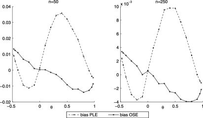
(b) Approximations (based on 15,000 replications) to the biases $\mathbb{E}_{\theta}[\hat{\theta}_{n}^{\mathrm{PLE}}]-\theta$ and

$\mathbb{E}_{\theta}[\hat{\theta}_{n}^{\mathrm{OSE}}]-\theta$ as a function of $\theta$.

Figure 2: Simulation results for the exchangeable model of Example 5.3 in dimension $p=3$ for $\theta\in\{-0.475,-0.45\}\cup\{k/10|k=-4,\ldots,9\}\cup\{0.95,0.975\}$ and $n\in\{50,250\}$.

To assess the impact of the dimension, we also compare the one-step and pseudo-likelihood estimators in dimension $p=100$ for 15,000 Monte Carlo samples of size $n=50$ at $\theta=0.25$. Boxplots of the estimation errors are shown in Figure E.2 in the supplement. Although the variances of both estimators are about the same, the pseudo-likelihood estimator suffers from a large bias, whereas the one-step estimator remains centered around the true value.

Example 5.4 ((Circular model)).

In Hoff, Niu and Wellner (2014), the four-dimensional circular model

$$R(\theta)=\pmatrix{1&\theta&\theta^{2}&\theta\vspace*{2pt}\cr\theta&1&\theta&\theta^{2}\vspace*{2pt}\cr\theta^{2}&\theta&1&\theta\vspace*{2pt}\cr\theta&\theta^{2}&\theta&1},\qquad-1<\theta<1,$$

is introduced as a one-parameter Gaussian copula model where the pseudo-likelihood estimator is not efficient. The optimal asymptotic variance if margins are unknown, the asymptotic variance of the pseudo-likelihood estimator, and the inverse Fisher information if margins are known can be computed explicitly:

$$I^{-1}(\theta) = \frac{I^{*-1}(\theta)}{1+2\theta^{2}}\leq I^{*-1}(\theta)=\frac{1}{4}\bigl{(}1-\theta^{2}\bigr{)}^{2}$$

$$\leq I^{*-1}(\theta)\biggl{(}1+\frac{2\theta^{6}}{(1+2\theta^{2})^{2}}\biggr{)}=\sigma^{2}_{\mathrm{PLE}}.$$

Even though the pseudo-likelihood estimator is not efficient, its asymptotic relative efficiency is close to $100\%$, except for $\theta$ close to $1$ or $-1$. Adaptivity occurs at independence ($\theta=0$) only.

We assessed the finite-sample performance of the one-step and pseudo-likelihood estimators by 15,000 Monte Carlo samples of sizes $n=50$ and $n=250$ for $\theta$ in a grid of values between $-1$ and $1$. The results are comparable to those for the exchangeable model: see Figures E.3–E.4 in the supplement.

Example 5.5 ((Factor models)).

Factor models are a popular tool for dimension reduction. In dimension $p\geq 3$, set

$$\mathbf{Z}=\theta\mathbf{W}+\bigl{(}I_{p}-\operatorname{diag}\bigl{(}\theta\theta^{\prime}\bigr{)}\bigr{)}^{1/2}\bolds{\varepsilon},$$ (44)

where $\theta$ denotes a $p\times q$ matrix, $q<p$, and where $\mathbf{W}$ and $\bolds{\varepsilon}$ are independent random vectors of dimensions $q$ and $p$, respectively, such that $(\mathbf{W}^{\prime},\bolds{\varepsilon}^{\prime})^{\prime}\sim N_{q+p}(\mathbf{0},I_{p+q})$. The parameter space $\Theta$ is an open subset of $\{\theta\in\mathbb{R}^{p\times q}|(\theta\theta^{\prime})_{jj}<1,j=1,\ldots,p\}$; in particular, $I_{p}-\operatorname{diag}(\theta\theta^{\prime})$ is a diagonal matrix with positive elements on the diagonal. As the variance matrix of $\mathbf{Z}$ is a correlation matrix, (44) defines a Gaussian copula model with

$$R(\theta)=\theta\theta^{\prime}+\bigl{(}I_{p}-\operatorname{diag}\bigl{(}\theta\theta^{\prime}\bigr{)}\bigr{)}=I_{p}+\mathrm{rd}\bigl{(}\theta\theta^{\prime}\bigr{)}$$ (45)

in terms of the diagonal-removal operator $\mathrm{rd}(A)=A-\operatorname{diag}(A)$ for $A\in\mathbb{R}^{p\times p}$. The parameter $\theta$ is not identifiable: if $O$ is an orthogonal $q\times q$ matrix, then $R(\theta O)=R(\theta)$. Still, by Corollary D.2 in Appendix D, we may study efficiency of the pseudo-likelihood estimator for the parameter $\nu$ in any reparametrization $\nu\mapsto\theta(\nu)$ satisfying Assumption D.1, which makes the model identified, by the criterion in Theorem 4.1. After some calculations, which are detailed in the Appendix, the criterion can be shown to be satisfied, confirming the efficiency of the pseudo-likelihood estimator for Gaussian factor copula models.

Example 5.6 ((Adaptivity)).

Proposition 4.8 gives a necessary and sufficient criterion for adaptivity of a Gaussian copula model at a certain value of $\theta$. Adaptivity always occurs at the independence copula but, apart from this, is the exception rather than the rule. With some trial and error, other (artificial) examples can be constructed. For instance, the one-parameter model in dimension $p=3$ given by $R_{12}(\theta)=R_{13}(\theta)=\theta^{2}+0.5$ and $R_{23}(\theta)=\theta+0.25$, for $\theta$ in a neighborhood of $0$, can be verified to be adaptive at $\theta=0$.

6 Conclusion and extensions

The present paper provides a semiparametrically efficient, rank-based estimator for the copula parameter in structured Gaussian copula models under mild conditions on the parametrization $\theta\mapsto R(\theta)$ of the correlation matrix. This gives a positive answer to the conjecture formulated in Hoff, Niu and Wellner (2014) that in Gaussian copula models, semiparametrically efficient, rank-based estimators do exist. The estimator is based on the analysis of the tangent space structure of the model and the explicit calculation of the efficient score function. Simulations indicate that the large-sample distribution provides an accurate approximation to the finite-sample distribution of the estimator, even in large dimensions.

Moreover, we show that inference in structured Gaussian copula models can be studied using a convenient finite-dimensional algebraic representation of relevant scores and influence functions. This leads to straightforward conditions to verify the regularity or the efficiency of existing estimators. In particular, we provide a convenient necessary and sufficient condition for the semiparametric efficiency of the pseudo-likelihood estimator. It follows, for example, that this estimator is efficient in models that exhibit a suitable factor structure. However, we also provide examples where its relative efficiency can be as low as $20\%$. Several other concrete examples complement the analysis.

6.1 Other copulas

A natural question is how to perform rank-based, semiparametrically efficient inference in general semiparametric copula models. The Bickel–Le Cam technique of a one-step update based on a suitable pilot estimate should work in general, too. However, our derivation of the efficient score function and information matrix (Proposition 2.8) and the proof of the asymptotic normality of the estimator (Theorem 3.2) heavily relied on the Gaussian-copula assumption, by which all relevant score and influence functions are quadratic forms in the Gaussianized observations. In general, one will have to pass through the Sturm–Liouville equations in (A.11) in the supplement.

Another point of concern is what happens if the model is misspecified. Suppose, for instance, that the true copula is elliptical with a correlation matrix $R(\theta)$. Then the Gaussian quasi-score $\dot{\ell}_{\theta}$ in (4) will still be centered, and statistical inference procedures derived from it can be expected to be $\sqrt{n}$-consistent. Semiparametric efficiency will be lost, however, since the structure of the tangent space will have changed.

6.2 Regression models

An important application of (Gaussian) copula models lies in joint regression analyses [Song (2000), Song, Li and Yuan (2009), Masarotto and Varin (2012)]. Consider a generalized linear model for each component of a vector of dependent variables $\mathbf{Y}=(Y_{1},\ldots,Y_{p})$. The vector of covariates, $\mathbf{X}$, is common to each of the $p$ model equations. Assume that the joint distribution of the vector of error variables $(\varepsilon_{1},\ldots,\varepsilon_{p})$ in the $p$ model equations has copula $C_{\theta}$ with unknown parameter vector $\theta$. The joint conditional distribution of $\mathbf{Y}$ given $\mathbf{X}$ is then parametrically specified. Estimating the $p$ vectors of regression parameters jointly with $\theta$, for instance, by maximum likelihood, is potentially more efficient than fitting each of the $p$ univariate models separately.

The question is what happens in the semiparametric context, when the marginal distributions of the errors $\varepsilon_{j}$ are left unspecified, except for a restriction to identify the model parameters. Does joint modeling still lead to more efficient inference on the regression coefficients? Is it still possible to estimate the (Gaussian) copula parameter efficiently using ranks?

We illustrate the possibilities and difficulties by means of a simple example. Consider a bivariate “dependent” variable $\mathbf{Y}=(Y_{1},Y_{2})$ and a univariate “explanatory” variable $X$. The precise setup is described by

$$Y_{j}=\beta_{j}X+\alpha_{j}+\varepsilon_{j},\qquad j\in\{1,2\},$$

where $\varepsilon_{j}=F_{j}^{-1}(\Phi(Z_{j}))$, for $j\in\{1,2\}$, with $(Z_{1},Z_{2})$ bivariate standard normal with correlation $\theta\in(-1,1)$ and $F_{1},F_{2}\in\mathcal{F}_{\mathrm{ac}}$ with absolutely continuous densities $f_{1},f_{2}$, respectively. The model parameters are identified by imposing a location restriction on $F_{1}$ and $F_{2}$; for instance, their means or their medians should be zero. We assume that $X$, with $0<\operatorname{var}X<\infty$, is independent of $(Z_{1},Z_{2})$, has an unknown density $f_{X}$ w.r.t. some dominating measure, and is exogenous, that is, its distribution does not depend on $(\alpha_{1},\alpha_{2},\beta_{1},\beta_{2},\theta,F_{1},F_{2})$. Finally, we assume that $f_{1}$ and $f_{2}$ have finite Fisher information for location, that is, $\int[(f_{j}^{\prime}(x))^{2}/f_{j}(x)]\,\mathrm{d}x<\infty$ for $j\in\{1,2\}$.

We are both interested in efficient inference about the copula parameter $\theta$ and about the regression coefficients $\beta_{1}$ and $\beta_{2}$, in the presence of the nuisance parameters $\alpha_{1}$, $\alpha_{2}$, $f_{1}$, and $f_{2}$. We follow the tangent space calculations as in Section 2. Conditionally on $X$, the joint distribution of $\mathbf{Y}$ has a bivariate Gaussian copula $C_{\theta}$ with correlation parameter $\theta$. The density of $(\mathbf{Y},X)$ is given by

$$(y_{1},y_{2},x) \mapsto c_{\theta}\bigl{(}F_{1}(y_{1}-\alpha_{1}-\beta_{1}x),F_{2}(y_{2}-\alpha_{2}-\beta_{2}x)\bigr{)}$$

$${}\times f_{1}(y_{1}-\alpha_{1}-\beta_{1}x)f_{2}(y_{2}-\alpha_{2}-\beta_{2}x)f_{X}(x).$$

The scores of the Euclidean parameters are given by

$$\dot{\ell}_{\theta}(\mathbf{Y},X) = \frac{\mathrm{d}}{\mathrm{d}\theta}\log c_{\theta}\bigl{(}F_{1}(\varepsilon_{1}),F_{2}(\varepsilon_{2})\bigr{)},$$ (46)

$$\dot{\ell}_{\alpha_{j}}(\mathbf{Y},X) = -\dot{\ell}_{j}\bigl{(}F_{1}(\varepsilon_{1}),F_{2}(\varepsilon_{2});\theta\bigr{)}f_{j}(\varepsilon_{1})-\frac{f_{j}^{\prime}}{f_{j}}(\varepsilon_{1}),$$ (47)

$$\dot{\ell}_{\beta_{j}}(\mathbf{Y},X) = X\dot{\ell}_{\alpha_{j}}(\mathbf{Y},X),$$ (48)

for $j\in\{1,2\}$. Irrespective of the specific location restriction that is used to identify $\alpha_{1}$ and $\alpha_{2}$, the set of distribution functions $G_{j}$ that are obtained as those of $\alpha_{j}+\varepsilon_{j}=Y_{j}-\beta_{j}X_{j}$ is unrestricted. As a consequence, the tangent space generated by the nuisance parameters $\alpha_{1}$, $\alpha_{2}$, $f_{1}$ and $f_{2}$ is equal to the collection of the score functions $s(Y_{1}-\beta_{1}X_{1},Y_{2}-\beta_{2}X_{2})$ with $s$ in $\mathcal{T}_{\mathrm{P}_{\theta,G_{1},G_{2}}}$ as in (2.3).

We first consider efficient estimation of the copula parameter $\theta$. As the score function for $\theta$ and the tangent space generated by the nuisance parameters $\alpha_{1}$, $\alpha_{2}$, $f_{1}$, and $f_{2}$ are, up to isometry, identical to those in Section 2, the efficient score for estimating $\theta$ in the presence of the nuisance parameters $\alpha_{1}$, $\alpha_{2}$, $f_{1}$, and $f_{2}$ remains $\dot{\ell}_{\theta}^{*}(F_{1}(\varepsilon_{1}),F_{2}(\varepsilon_{2});\theta)$. Given the independence of $X$ and $(\varepsilon_{1},\varepsilon_{2})$, the function $\dot{\ell}_{\theta}^{*}(F_{1}(\varepsilon_{1}),F_{2}(\varepsilon_{2});\theta)$ is automatically orthogonal to $\dot{\ell}_{\beta_{j}}(\mathbf{Y},X)=X\dot{\ell}_{\alpha_{j}}(\mathbf{Y},X)$, for $j\in\{1,2\}$.

These tangent space calculations show the possibility of efficient estimation of Gaussian copula parameters in joint regression analyses. A formal proof of efficiency of the OSE would be significantly complicated by the fact that one now has to rely on aligned ranks. That is, the ranks to be used for the computation of the initial estimator and the update step would be those of the residuals based on some initial estimates $\hat{\alpha}_{j}$ and $\hat{\beta}_{j}$, for $j\in\{1,2\}$. Techniques for this exist [Hallin, Vermandele and Werker (2006) and the references therein] but require subtle analysis of remainder terms.

Usually, the interest lies in the estimation of the regression parameters $\alpha_{j}$ and $\beta_{j}$ for $j\in\{1,2\}$. In order to identify $\alpha_{j}$, an identification restriction on the location of $f_{j}$ is needed. Focusing on rank-based procedures, a natural choice is to use a median restriction, that is, to impose $\int_{-\infty}^{0}f(x)\,\mathrm{d}x=1/2$. In univariate settings, this problem has been studied extensively and semiparametrically efficient inference procedures can be based on signs and ranks [Hallin, Vermandele and Werker (2006)].

Concerning the estimation of $\beta_{j}$, its efficient score is given by the residual of the projection of $\dot{\ell}_{\beta_{j}}(\mathbf{Y},X)$ on the tangent space generated by the score functions for $\alpha_{1},\alpha_{2},f_{1},f_{2}$ and $\beta_{3-j}$. Elementary calculations (see Appendix F in the supplement) show that this efficient score is given by

$$\dot{\ell}^{*}_{\beta_{j}}(Y,X)=(\dot{\ell}_{\alpha_{j}}-c_{j}\dot{\ell}_{\alpha_{3-j}})(X-\mathbb{E}X),$$ (49)

with $c_{j}=\operatorname{cov}(\dot{\ell}_{\alpha_{1}},\dot{\ell}_{\alpha_{2}})/\operatorname{var}(\dot{\ell}_{\alpha_{3-j}})$.

It is interesting to compare this efficient score to the univariate regression case, that is, to the case where only $(Y_{j},X)$ is observed. It is known [see Example 3 in Bickel (1982)] that in that case the efficient score is given by

$$-\frac{f_{j}^{\prime}}{f_{j}}(\varepsilon_{j})(X-\mathbb{E}X).$$ (50)

In general, the score functions in (49) and (50) do not coincide, which suggests that efficiency gains are possible from joint regression analyses. The numerical size of the gains would have to be investigated further. One interesting observation is that, at Gaussian marginals, the efficient score functions in (49) and (50) do coincide as, again, follows from straightforward calculations detailed in the supplement. This result is well-known from the literature on Seemingly Unrelated Regressions [see Chapter 12 in Davidson and MacKinnon (2004)], but does not extend to non-Gaussian distributions. Indeed, obtaining more efficient estimators of regression parameters by joint analyses using copulas was exactly the point in Song (2000) and Song, Li and Yuan (2009).

References

- Basrak and Klaassen (2013) {bincollection}[author] \bauthor\bsnmBasrak, \bfnmBojan\binitsB. and \bauthor\bsnmKlaassen, \bfnmChris A. J.\binitsC. A. J. (\byear2013). \btitleEfficient estimation in the semiparametric normal regression-copula model with a focus on QTL mapping. In \bbooktitleFrom Probability to Statistics and Back: High-Dimensional Models and Processes—A Festschrift in Honor of Jon A. Wellner (\beditor\bfnmM.\binitsM. \bsnmBanerjee, \beditor\bfnmF.\binitsF. \bsnmBunea, \beditor\bfnmJ.\binitsJ. \bsnmHuang, \beditor\bfnmV.\binitsV. \bsnmKoltchinskii and \beditor\bfnmM. H.\binitsM. H. \bsnmMaathuis, eds.) \bpages20–32. \bpublisherIMS, \blocationBeachwood, OH. \bidmr=3186746 \bptokimsref\endbibitem
- Bickel (1982) {barticle}[mr] \bauthor\bsnmBickel, \bfnmP. J.\binitsP. J. (\byear1982). \btitleOn adaptive estimation. \bjournalAnn. Statist. \bvolume10 \bpages647–671. \bidissn=0090-5364, mr=0663424 \bptokimsref\endbibitem
- Bickel et al. (1993) {bbook}[mr] \bauthor\bsnmBickel, \bfnmPeter J.\binitsP. J., \bauthor\bsnmKlaassen, \bfnmChris A. J.\binitsC. A. J., \bauthor\bsnmRitov, \bfnmYa’acov\binitsY. and \bauthor\bsnmWellner, \bfnmJon A.\binitsJ. A. (\byear1993). \btitleEfficient and Adaptive Estimation for Semiparametric Models. \bpublisherJohns Hopkins Univ. Press, \blocationBaltimore, MD. \bidmr=1245941 \bptokimsref\endbibitem
- Brahimi and Necir (2012) {barticle}[mr] \bauthor\bsnmBrahimi, \bfnmBrahim\binitsB. and \bauthor\bsnmNecir, \bfnmAbdelhakim\binitsA. (\byear2012). \btitleA semiparametric estimation of copula models based on the method of moments. \bjournalStat. Methodol. \bvolume9 \bpages467–477. \biddoi=10.1016/j.stamet.2011.11.003, issn=1572-3127, mr=2897802 \bptokimsref\endbibitem
- Chen, Fan and Tsyrennikov (2006) {barticle}[mr] \bauthor\bsnmChen, \bfnmXiaohong\binitsX., \bauthor\bsnmFan, \bfnmYanqin\binitsY. and \bauthor\bsnmTsyrennikov, \bfnmViktor\binitsV. (\byear2006). \btitleEfficient estimation of semiparametric multivariate copula models. \bjournalJ. Amer. Statist. Assoc. \bvolume101 \bpages1228–1240. \biddoi=10.1198/016214506000000311, issn=0162-1459, mr=2328309 \bptokimsref\endbibitem
- Chen, Wu and Yi (2009) {barticle}[mr] \bauthor\bsnmChen, \bfnmXiaohong\binitsX., \bauthor\bsnmWu, \bfnmWei Biao\binitsW. B. and \bauthor\bsnmYi, \bfnmYanping\binitsY. (\byear2009). \btitleEfficient estimation of copula-based semiparametric Markov models. \bjournalAnn. Statist. \bvolume37 \bpages4214–4253. \biddoi=10.1214/09-AOS719, issn=0090-5364, mr=2572458 \bptokimsref\endbibitem
- Cheng et al. (2014) {barticle}[mr] \bauthor\bsnmCheng, \bfnmGuang\binitsG., \bauthor\bsnmZhou, \bfnmLan\binitsL., \bauthor\bsnmChen, \bfnmXiaohong\binitsX. and \bauthor\bsnmHuang, \bfnmJianhua Z.\binitsJ. Z. (\byear2014). \btitleEfficient estimation of semiparametric copula models for bivariate survival data. \bjournalJ. Multivariate Anal. \bvolume123 \bpages330–344. \biddoi=10.1016/j.jmva.2013.10.008, issn=0047-259X, mr=3130438 \bptokimsref\endbibitem
- Davidson and MacKinnon (2004) {bbook}[author] \bauthor\bsnmDavidson, \bfnmRussell\binitsR. and \bauthor\bsnmMacKinnon, \bfnmJames G.\binitsJ. G. (\byear2004). \btitleEconometric Theory and Methods. \bpublisherOxford Univ. Press, \blocationNew York. \bptokimsref\endbibitem
- Genest, Ghoudi and Rivest (1995) {barticle}[mr] \bauthor\bsnmGenest, \bfnmC.\binitsC., \bauthor\bsnmGhoudi, \bfnmK.\binitsK. and \bauthor\bsnmRivest, \bfnmL.-P.\binitsL.-P. (\byear1995). \btitleA semiparametric estimation procedure of dependence parameters in multivariate families of distributions. \bjournalBiometrika \bvolume82 \bpages543–552. \biddoi=10.1093/biomet/82.3.543, issn=0006-3444, mr=1366280 \bptokimsref\endbibitem
- Genest and Rivest (1993) {barticle}[mr] \bauthor\bsnmGenest, \bfnmChristian\binitsC. and \bauthor\bsnmRivest, \bfnmLouis-Paul\binitsL.-P. (\byear1993). \btitleStatistical inference procedures for bivariate Archimedean copulas. \bjournalJ. Amer. Statist. Assoc. \bvolume88 \bpages1034–1043. \bidissn=0162-1459, mr=1242947 \bptokimsref\endbibitem
- Genest and Werker (2002) {bincollection}[mr] \bauthor\bsnmGenest, \bfnmChristian\binitsC. and \bauthor\bsnmWerker, \bfnmBas J. M.\binitsB. J. M. (\byear2002). \btitleConditions for the asymptotic semiparametric efficiency of an omnibus estimator of dependence parameters in copula models. In \bbooktitleDistributions with Given Marginals and Statistical Modelling (\beditor\bfnmC. M.\binitsC. M. \bsnmCuadras and \beditor\bfnmJ. A. Rodríguez\binitsJ. A. R. \bsnmLallena, eds.) \bpages103–112. \bpublisherKluwer Academic, \blocationDordrecht. \bidmr=2058984 \bptokimsref\endbibitem
- Gordon (1941) {barticle}[mr] \bauthor\bsnmGordon, \bfnmRobert D.\binitsR. D. (\byear1941). \btitleValues of Mills’ ratio of area to bounding ordinate and of the normal probability integral for large values of the argument. \bjournalAnn. Math. Statistics \bvolume12 \bpages364–366. \bidissn=0003-4851, mr=0005558 \bptokimsref\endbibitem
- Hallin, Vermandele and Werker (2006) {barticle}[mr] \bauthor\bsnmHallin, \bfnmMarc\binitsM., \bauthor\bsnmVermandele, \bfnmCatherine\binitsC. and \bauthor\bsnmWerker, \bfnmBas\binitsB. (\byear2006). \btitleSerial and nonserial sign-and-rank statistics: Asymptotic representation and asymptotic normality. \bjournalAnn. Statist. \bvolume34 \bpages254–289. \biddoi=10.1214/009053605000000769, issn=0090-5364, mr=2275242 \bptokimsref\endbibitem
- Hobæk Haff (2013) {barticle}[mr] \bauthor\bsnmHobæk Haff, \bfnmIngrid\binitsI. (\byear2013). \btitleParameter estimation for pair-copula constructions. \bjournalBernoulli \bvolume19 \bpages462–491. \biddoi=10.3150/12-BEJ413, issn=1350-7265, mr=3037161 \bptokimsref\endbibitem
- Hoff (2007) {barticle}[mr] \bauthor\bsnmHoff, \bfnmPeter D.\binitsP. D. (\byear2007). \btitleExtending the rank likelihood for semiparametric copula estimation. \bjournalAnn. Appl. Stat. \bvolume1 \bpages265–283. \biddoi=10.1214/07-AOAS107, issn=1932-6157, mr=2393851 \bptokimsref\endbibitem