Current Sheets Formation in Tangled Coronal Magnetic Fields

Abstract

We investigate the dynamical evolution of magnetic fields in closed regions of solar and stellar coronae. To understand under which conditions current sheets form, we examine dissipative and ideal reduced magnetohydrodynamic models in cartesian geometry, where two magnetic field components are present: the strong guide field $B_{0}$, extended along the axial direction, and the dynamical orthogonal field $\mathbf{b}$. Magnetic field lines thread the system along the axial direction, that spans the length $L$, and are line-tied at the top and bottom plates. The magnetic field $b$ initially has only large scales, with its gradient (current) length-scale of order $\ell_{b}$. We identify the magnetic intensity threshold $b/B_{0}\sim\ell_{b}/L$. For values of $b$ below this threshold, field-line tension inhibits the formation of current sheets, while above the threshold they form quickly on fast ideal timescales. In the ideal case, above the magnetic threshold, we show that current sheets thickness decreases in time until it becomes smaller than the grid resolution, with the analyticity strip width $\delta$ decreasing at least exponentially, after which the simulations become under-resolved.

1. Introduction

All late type main sequence stars, for which the Sun is the prototype, emit X-rays (Güdel, 2004). And solar observations at increasingly higher resolutions show that the X-ray corona has structures at all resolved scales (Cirtain et al., 2013).

Convective motions, that have more than enough energy to heat the corona at temperatures $>10^{6}\,\textrm{K}$, shuffle continuously the coronal magnetic field line footpoints, giving rise to a magnetic field that is not in equilibrium (Parker, 1972, 2000; van Ballegooijen, 1985). Parker (1972, 1988, 1994, 2012) pointed out that current sheets are an intrinsic part of the final equilibrium of almost all interlaced field line topologies. So the asymptotic relaxation of the interlaced field to equilibrium necessarily involves the formation of current sheets, providing energy dissipation presumably concentrated in small impulsive heating events, so-called nanoflares. This picture has had a strong impact on the thermodynamical modeling of the closed corona (Klimchuk, 2006), but it is still controversial if and under which circumstances current sheets form.

Analytical models (van Ballegooijen, 1985; Antiochos, 1987; Cowley et al., 1997) claim that in general well-behaved photospheric motions will not lead to the formation of current sheets, and that only a discontinuous velocity field can form discontinuities in the coronal magnetic field, and counterexamples of well-behaved solutions of the magnetostatic equations have been reported (Rosner & Knobloch, 1982; Bogoyavlenskij, 2000).

Alternatively van Ballegooijen (1986) proposed that the random character of footpoint motions might generate, on time-scales much longer than photospheric convection time-scales, uniformly distributed small-scale current layers that would heat the corona without forming discontinuous structures.

Numerical simulations of boundary forced models (Einaudi et al., 1996; Dmitruk & Gómez, 1997; Rappazzo et al., 2007) suggest that the nonlinear dynamics of this system can be modeled as a magnetically dominated instance of magnetohydrodynamic (MHD) turbulence, implicitly implying that current sheets thickness is limited only by numerical diffusion (i.e., resolution) in dissipative MHD. But recent simulations of the decay of an initially braided magnetic configuration (Wilmot-Smith et al., 2009) have shown that in some instances the system forms only large-scale current layers of thickness much larger than the resolution scale, in stark contrast with the recent result supporting the development of finite time singularities in the cold plasma regime (Low, 2013).

Furthermore, recent investigations suggest that the rate of magnetic reconnection can be very fast in low collisional plasmas, both in the MHD (Lazarian & Vishniac, 1999; Lapenta, 2008; Loureiro et al., 2009; Huang & Bhattacharjee, 2010) and the collisionless regime (Shay et al., 1999). Therefore, in order to have an X-ray corona, it is critical that current sheets form, but only above a magnetic energy threshold. Indeed the energy flux injected in the corona by photospheric motions is the average Poynting flux $\langle S_{z}\rangle=B_{0}\,\langle\mathbf{u}_{\textrm{ph}}\cdot\mathbf{b}\rangle/4\pi$ (Rappazzo et al., 2008, §3.1), that depends not only on the photospheric velocity $\mathbf{u}_{\textrm{ph}}$ and the axial guide field $B_{0}$, but also on the dynamic magnetic field $\mathbf{b}$, and if dissipation keeps low the value of $b$, the flux $\langle S_{z}\rangle$ will be too low to sustain the corona (Withbroe & Noyes, 1977).

In this letter we investigate, in a cartesian model of the closed corona, under which conditions current sheets form, and their dynamical properties.

2. Model

A closed region of the solar corona is modeled in cartesian geometry as a plasma with uniform density $\rho_{0}$ embedded in a strong and homogeneous axial magnetic field $\mathbf{B}_{0}=B_{0}\,\mathbf{\hat{e}}_{z}$ well suited to be studied (e.g., see Dahlburg et al., 2012), as in previous work, with the equations of reduced magnetohydrodynamics (RMHD). Introducing the velocity and magnetic field potentials $\varphi$ and $\psi$, for which $\mathbf{u}=\nabla\times\left(\varphi\,\mathbf{\hat{e}}_{z}\right)$, $\mathbf{b}=\nabla\times\left(\psi\,\mathbf{\hat{e}}_{z}\right)$, vorticity $\omega=-\nabla^{2}_{\!{}_{\!\perp}}\varphi$, and the current density $j=-\nabla^{2}_{\!{}_{\!\perp}}\psi$, the nondimensional RMHD equations (Kadomtsev & Pogutse, 1974; Strauss, 1976) are:

$$\partial_{t}\psi=\left[\varphi,\psi\right]+B_{0}\,\partial_{z}\varphi+\eta_{{}_{n}}\nabla_{{}_{\!\!\perp}}^{2n}\psi,\quad$$ (1)

$$\partial_{t}\omega=\left[j,\psi\right]-\left[\omega,\varphi\right]+B_{0}\,\partial_{z}j+\nu_{{}_{\!n}}\nabla_{{}_{\!\!\perp}}^{2n}\omega,$$ (2)

The Poisson bracket of functions $g$ and $h$ is defined as $[g,h]=\partial_{x}g\,\partial_{y}h-\partial_{y}g\,\partial_{x}h$ (e.g., $[j,\psi]=\mathbf{b}\cdot\nabla j$), and Laplacian operators have only orthogonal components. To render the equations nondimensional we have first expressed the magnetic fields as an Alfvén velocity ($b\rightarrow b/\sqrt{4\pi\rho_{0}}$) and then normalized all velocities to $u^{\ast}=1$ km s^-1, typical value for the photosphere. The domain spans $0\leq x,y,\leq\ell$, $0\leq z\leq L$, with $\ell=1$ and $L=10$. Magnetic field lines are line-tied to a motionless photosphere at the top and bottom plates $z=0,10$, where a velocity $\mathbf{u}=0$ is imposed. In the perpendicular ($x$-$y$) directions we use a pseudo-spectral scheme with periodic boundary conditions, and along $z$ a second-order finite difference scheme. For a more detailed description of the model and numerical code see Rappazzo et al. (2007, 2008).

Dissipative simulations use hyper-diffusion (Biskamp, 2003), that effectively limits diffusion to the small scales, with $n=4$ and $\nu_{n}=\eta_{n}=\left(-1\right)^{n+1}/R_{n}$ ($R_{n}$ corresponds to the Reynolds number for $n=1$) (see Rappazzo et al., 2008, §2.1), while ideal simulations implement $\nu_{n}=\eta_{n}=0$.

2.1. Initial conditions

Simulations are started at time $t=0$ with a vanishing velocity $\mathbf{u}=0$ everywhere, and a uniform and homogeneous guide field $B_{0}$. The orthogonal field $\mathbf{b}$ consists of large-scale Fourier modes, set expanding the magnetic potential in the following way:

$$\psi_{0}=b_{0}\sum_{rsm}(2\mathscr{E}_{{}_{m}})^{\frac{1}{2}}\ \frac{\alpha_{rsm}\ \sin\left(\mathbf{k}_{rsm}\!\cdot\mathbf{x}+2\pi\xi_{rsm}\right)}{k_{rs}\ \sqrt{\sum_{ij}\alpha^{2}_{ijm}}}$$ (3)

$$\textrm{with}\quad\mathbf{k}_{rsm}=\frac{2\pi}{\ell}\left(r\,\mathbf{\hat{e}}_{x}+s\,\mathbf{\hat{e}}_{y}\right)+\frac{2\pi}{L}m\,\mathbf{\hat{e}}_{z},$$

$$\textrm{and}\quad k_{rs}=\frac{2\pi}{\ell}\sqrt{r^{2}+s^{2}},$$

where the coefficients $\alpha_{rsm}$ and $\xi_{rsm}$ are two independent sets of random numbers uniformly distributed between 0 and 1. The orthogonal wave-numbers $(r,s)$ are always in the range $3\leq(r^{2}+s^{2})^{1/2}\leq 4$, while the parallel amplitudes $\mathscr{E}_{m}$ (with $\sum_{m}\mathscr{E}_{m}=1$) are set to distribute the energy in different ways in the axial direction. Given the orthogonality of the base used in Eq. (3) the normalization factors guarantee that for any choice of the amplitudes the rms of the magnetic field is set to $b=\langle b_{x}^{2}+b_{y}^{2}\rangle^{1/2}=b_{0}$, while for total magnetic energy $E_{{}_{\!M}}=b_{0}^{2}V/2\sum_{m}\mathscr{E}_{m}$, i.e., $\mathscr{E}_{m}$ is the fraction of magnetic energy in the parallel mode $m$. Two-dimensional (2D) configurations invariants along $z$ are obtained considering the single mode $m=0$ with $\mathscr{E}_{0}=1$.

2.2. Equilibria

Neglecting velocity and diffusion, equilibria of Eqs. (1)-(2) are given by

$$\mathbf{b}\cdot\nabla j+B_{0}\partial_{z}j=0\quad\rightarrow\quad\partial_{z}j=-\mathbf{b}/B_{0}\cdot\nabla j.$$ (4)

This equation has the same structure of the 2D Euler equation for vorticity (van Ballegooijen, 1985), as can be verified substituting $(\mathbf{b}/B_{0},\ j/B_{0})\rightarrow(\mathbf{u},\ \omega)$, and $z$ with time $t$, and has been studied extensively in 2D hydrodynamic turbulence (Kraichnan & Montgomery, 1980). Given a smooth $j$ at any $x$-$y$ plane it admits a unique and regular solution (not singular, Rose & Sulem, 1978), with an asymmetric structure along $z$, as $\bf b$ acquires larger scales through an inverse cascade, and currents are stretched (with $j$ constant along the “fluid element”). Parker (2000, 2012) points out that the observed disordered photospheric motions will in general induce an interlaced coronal magnetic field that does not have this structure and will thus generally not be in equilibrium.

Given the long time-scale of photospheric convection respect to the fast Alfvén crossing time the coronal structure will be dominated by the low-frequency $m=0$ mode. In this 2D limit the equilibrium condition (4) reduces to $\mathbf{b}\cdot\nabla j=0$, i.e., $j$ is constant over the field lines of $\mathbf{b}$, a configuration too symmetric to occur in coronal fields.

We therefore use as initial condition a magnetic field that is not in equilibrium, obtained using random amplitudes in our initial conditions (3) (a 2D example is shown in Figure 5, $t=0$).

3. Results

We first consider initial conditions with $m=0$ (not in equilibrium, with field lines of $\mathbf{b}$ same as in Figure 5 at $t=0$), invariant along the axial direction ($\partial_{z}=0$), and $b_{0}=0.1B_{0}$, with $B_{0}=10^{3}$. To understand the effect of line-tying we perform two dissipative sets of simulations with same parameters but different boundary conditions along $z$: periodic (with $R_{4}=3\cdot 10^{20}$ and a $1024^{2}\times 512$ grid), and line-tied (with $R_{4}=10^{19}$ and $512^{2}\times 256$ grids).

The periodic case is the limit of a very long loop, when line-tying boundary conditions do not have a strong bearing on the dynamics. In this case the system is approximately invariant along $z$, and the solution will be two-dimensional as the initial condition ($\partial_{z}=0$). This configuration is akin to 2D turbulence decay (Biskamp, 2003; Hossain et al., 1995), except that the initial velocity vanishes.

At $t=0$ the magnetic field is not in equilibrium, thus no instability develops, but the non-vanishing Lorentz force transfers $\sim 15\%$ of magnetic energy $E_{M}$ into kinetic energy $E_{K}$ (with $E_{M}$ bigger than $E_{K}$ in all simulations), while until time $t\sim 0.3\,\tau_{A}$ total energy $E$ is conserved (Figure 1). Subsequently magnetic energy, initially present only in perpendicular modes $k=3$ and $4$, cascades in Fourier space toward higher wavenumbers (Figure 1, inset, $E=\sum_{k}E_{k}$), corresponding to the formation of current sheets in physical space. At the peak of dissipation ($t\sim 1.7\,\tau_{A}$) the spectrum exhibits a $k^{-3/2}$ power-law and is fully extended toward the maximum wavenumber ($k_{\textrm{max}}=341$).

Figure 1.— Periodic simulation with 2D initial conditions: Magnetic $E_{M}$, Kinetic $E_{K}$ and total energies $E$ versus time (normalized with the initial total energy). Magnetic energy spectra at selected times are shown in the inset.

Once current sheets are formed dissipation occurs, total and magnetic energies decay approximately with the power-law $E\propto t^{-4/5}$ (see inset in Figure 2) as in the 2D turbulence case (Galtier et al., 1997), while kinetic energy decays as $E_{K}\propto t^{-1}$ before vanishing asymptotically. The magnetic field loses energy at high wavenumbers (Figure 1, inset $t=60\,\tau_{A}$), thus current sheets disappear, and the system relaxes to a stage with $\sim 5\%$ of the initial magnetic energy and a very small velocity. At the same time an inverse cascade occurs, transferring energy at the largest scales (particularly in mode $k=1$), so that the asymptotic state consists of large-scale magnetic islands, with large-scale current layers and no current sheets, and this process can be described as the 2D analog of Taylor relaxation (Taylor, 1986).

For this 2D case (periodic boundary conditions, with $\partial_{z}=0$) given a solution of Eqs. (1)-(2) with initial condition $b=b_{0}$, solutions with $b=\sigma b_{0}$ and same random amplitudes are self-similar in time: $\psi_{\sigma}(\mathbf{x},t)=\sigma\,\psi_{0}(\mathbf{x},\sigma\,t)$. Consequently all these solutions have a similar structure and the temporal evolution differs only for the scaling factor $\sigma$. In particular if current sheets form for a certain value of $b_{0}$, they will always do for any value of $b_{0}$ at scaled times. Analogously energy will exhibit a power-law decay with the same exponent as $E_{\sigma}(t)=\sigma^{2}E_{0}(\sigma t)$.

When the same initial condition is used with line-tying boundary conditions, the system is no longer invariant along $z$, as now the velocity must vanish at the top and bottom plates $z=0,L$, therefore the velocity cannot develop uniformly along z as in the periodic case.

The temporal evolution of total energy for line-tied simulations with different values of $b_{0}$ is shown in Figure 2. While the dynamics of the system with $b_{0}/B_{0}=10\%$ is similar to the 2D case with energy dissipating $\sim 80\%$ of its initial value, the behavior is increasingly different for lower values of $b_{0}$, with less energy getting dissipated. For $b_{0}/B_{0}\lesssim 3\%$ no significant energy dissipation nor decay are observed, and also for the decaying cases their dynamics are quenched once energy crosses this threshold. As shown in the inset in Fig. 2 energies decay with different power-law indices, indicating that self-similarity is lost and new dynamics emerge.

There are therefore two antagonistic forces at work. The system starts to behave as in the 2D case, with the tension of perpendicular field lines $\mathbf{b}\cdot\nabla\mathbf{b}$ creating an orthogonal velocity, that coupled with all others nonlinear terms are the only ones that can cascade energy and generate current sheets. But this displaces the total line-tied (axially directed) field lines, and is then opposed by the axial tension $B_{0}\partial_{z}\mathbf{b}$ that resists bending, and together with the other linear term $\propto B_{0}\partial_{z}$ tends to impose the vanishing boundary velocity in the whole box. Furthermore the pattern of the boundary velocity does not match that of the velocity generated by the nonlinear terms in Eqs. (1)-(2) (also for $\mathbf{u}_{\textrm{ph}}\neq 0$). Consequently line-tying opposes current sheet formation, more efficiently the smaller the value of $b/B_{0}$.

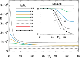
Figure 2.— Total magnetic energy versus time (in logarithmic scale in the inset) for line-tied simulations with different values of $b_{0}/B_{0}$, and the 2D simulation with $b_{0}/B_{0}=10\%$.

For a low ratio of $b_{0}/B_{0}$ the axial field line tension dominates and impedes the formation of current sheets. This is quantitatively shown in Fig. 3. Magnetic Taylor microscale $\lambda_{T}=(\langle b^{2}\rangle/\langle j^{2}\rangle)^{1/2}$ measures the average length-scale of magnetic gradients (Matthaeus et al., 2005). The smallest scales are reached in the 2D simulation, while for the line-tied case the minimum value of $\lambda_{T}$ increases with $b_{0}/B_{0}$, but for $b_{0}/B_{0}<4\%$ no significant gradients are formed. While the 2D case retains larger gradients in the asymptotic state, line-tying sharply removes small-scales after the dissipative peak. At the same time normalized energy dissipation rate $\epsilon/E$ ($\epsilon=dE/dt$) decreases sharply for lower values of $b_{0}/B_{0}$, with the 2D case reaching a higher dissipative peak.

We have performed similar sets of simulations with different initial conditions, including more modes besides $m=0$, and they show a similar behavior to that shown in Figs. 1-3 and will be described in detail in an upcoming paper.

We conclude that current sheets form when the orthogonal Lorentz force $\mathbf{b}\cdot\nabla\mathbf{b}$ is stronger than the field line tension term $B_{0}\partial_{z}\mathbf{b}$. From initial condition (3) we can estimate the gradient lenght-scale of $b$ in the orthogonal direction as $\ell_{b}\sim\ell/3.5$, while line-tying will yield a lenght-scale of $\sim L$ for the variation of $b$ along $z$. We can therefore estimate:

$$\frac{b}{\ell_{b}}\gtrsim\frac{B_{0}}{L}\quad\longrightarrow\quad\frac{b}{B_{0}}\gtrsim\frac{\ell}{3.5\,L}$$ (5)

With the values used in our simulations ($\ell=1,L=10$) this rough estimate yields $b/B_{0}\gtrsim 3\%$, in agreement with the simulations presented here, and this is also approximately the level to which fluctuations settle in the forced case (Rappazzo et al., 2008).

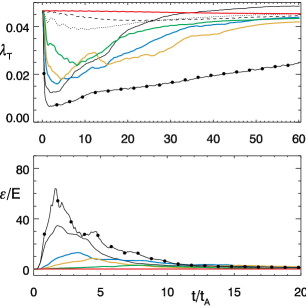
Figure 3.— Taylor microscale $\lambda_{T}$ and normalized energy dissipation rate $\epsilon/E$ ($\epsilon=dE/dt$) versus time. Color codes same as in Figure 2.

3.1. Ideal simulations

Current sheet formation if further analyzed with two ideal simulations of Eqs. (1)-(2), with $\eta_{n}=\nu_{n}=0$, $4096^{2}\times 2048$ grids, $b_{0}/B_{0}=10\%,B_{0}=200$, and two different initial conditions, one with just the mode $m=0$, and the other one with all modes between 0 and 4 excited, with lower modes dominating ($\mathscr{E}_{{}_{m}}/\mathscr{E}_{{}_{0}}=(m+1)^{-2.6}$).

The analyticity-strip method (Sulem et al., 1983; Frisch et al., 2003; Brachet et al., 2013) extends to the complex space, off the real axis, the solutions of ideal MHD equations. Indicating with $\delta$ the distance from the real domain of the nearest complex space singularity, this determines in Fourier space an exponential fall-off at large $k$ for the power-law behavior of the total energy spectrum (of the real solutions):

$$E(k,t)=C(t)\,k^{-n(t)}\,e^{-2\delta(t)k}.$$ (6)

The width of the strongest current sheet is therefore linked to $\delta$, and if and how $\delta$ approaches the smallest admissible scale (fixed at $2$ meshes: $2/k_{\textrm{max}},k_{\textrm{max}}=1364$), determines whether or not true current sheets form and if the solution develops singularities (Sulem et al., 1983; Frisch et al., 2003; Krstulovic et al., 2011; Bustamante & Brachet, 2012).

For the case with $m=0$, initially $\delta$ decreases exponentially until time $t\sim 0.16\tau_{A}$ (Fig. 4), after which it obeys $\delta(t)=C(t_{\ast}-t)^{\gamma}$ with $t_{\ast}=0.26\tau_{A}$ and $\gamma=3.7$, crossing the resolution scale at $t\sim 0.2\tau_{A}$, with a singular-like behavior at $t=t_{\ast}$. The width $\delta(t)$ is determined fitting the spectrum with Eq. (6), while $t_{\ast}$ and $\gamma$ fit the inverse logarithmic derivative $\delta/\delta^{\prime}$ (Brachet et al., 2013), with a good linear behavior in this interval.

The spectral index $n(t)\sim 3.3$, with a maximum value of $\sim 3.7$, thus $\gamma$ satisfies the condition $\gamma\geq 2/(6-n)\sim 0.87$ that rules out numerical artifacts (Bustamante & Brachet, 2012; Brachet et al., 2013).

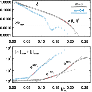
Figure 4.— Linear-logarithmic plot vs. time of the analyticity strip width $\delta$ and of the sum of the current density and vorticity (moduli) maxima, for the two ideal simulations with only mode $m=0$ and with modes $m=0$–4 present. The resolution scale is $2/k_{\textrm{max}}$.

Correspondingly the initially large-scale current density develops thin sheets with strong current enhancements (Fig. 5) that approach the resolution scale at $t\sim.2\tau_{A}$. Afterward $\delta$ becomes smaller than the mesh size, the field starts to develop gaussian statistics (Wan et al., 2009; Krstulovic et al., 2011), small-scale noise appears and the simulation becomes thus under-resolved.

The sum of the suprema of the absolute values of vorticity and current (Fig. 4) exhibits a double exponential behavior with fast growth rates ($\tau/\tau_{A}\sim 1/18$ and $1/46$ respectively), corresponding to two different leading current sheets. Thus no BKM (Beale, Kato, & Majda, 1984) power-law divergent behavior $C(t_{\ast}-t)^{-\beta}$, with $\beta\geq 1$, is detected. Therefore one of the three diagnostics for singularities is failed and a singular behavior cannot be established.

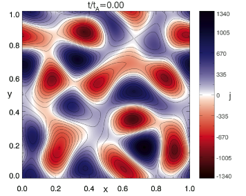
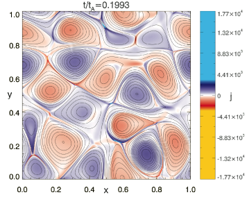
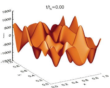
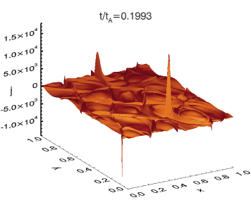
Figure 5.— Current density $j$ in the mid-plane $z=5$ for the simulation with $m=0$, at $t=0$ (left column) and at $t\sim.2\tau_{A}$ (right, the color scale reveals thin sheets with strong current enhancements) just before $\delta$ crosses the resolution scale (Fig. 4). Continuous lines are field lines of the orthogonal magnetic field.

When more axial modes are added to the initial condition, and the field has a three-dimensional structure, $\delta$ decreases faster, crossing the resolution threshold at $t\sim 0.125\tau_{A}$, and current and vorticity maxima have a higher exponential growth rate with $\tau/\tau_{A}\sim 1/52$.

4. Discussion

To get insight into the cause of the X-ray emission of the Sun and main sequence stars we have investigated the dynamical evolution of magnetic configurations (3) appropriate to model their coronal fields.

Provided the value of magnetic fluctuations $b$ is beyond the threshold (5), we have shown that current sheets form on fast ideal timescales, with their thickness reaching the resolution scale in the ideal case. Below this threshold the field-line tension of the line-tied magnetic field lines inhibits the dynamics and the formation of current sheets, thus the solutions remain regular. As mentioned in the introduction a current sheets formation threshold is a critical feature to sustain an X-ray corona.

The quasi-static dynamics of coronal fields is often modeled as a sequence of instabilities followed by relaxation and current sheets formation (Ng & Bhattacharjee, 1998), in which equilibria play an important role (Aly, 2005).

However the stability and dynamic accessibility of such equilibria require further investigations. Indeed the majority of these equilibria (Section 2.2) do not have the highly symmetric fields required for linear instability as, e.g., for kink or other cases (Longcope & Strauss, 1993). Furthermore the magnetic field induced by disordered photospheric motions is not symmetric, and in general will not be in equilibrium.

In our case the initial magnetic field is not an equilibrium. In the decaying cases no intermediate equilibria are accessed before current sheets form, and no instabilities develop. An approximate (non-symmetric) equilibrium is accessed only in the asymptotic regime of the dissipative simulations. A more complete analysis of the properties of these equilibria and their interplay with photospheric motions is left to upcoming work.

More in general, the current sheet formation threshold (5) might depend on the specific magnetic topology of the system.

References

- Aly (2005) Aly, J. J. 2005, A&A 429, 15
- Antiochos (1987) Antiochos, S. K. 1987, ApJ 312, 886
- Beale, Kato, & Majda (1984) Beale, J. T., Kato, T., and Majda, A. 1984, CMaPh 94, 61
- Biskamp (2003) Biskamp, D. 2003, Magnetohydrodynamic Turbulence (Cambridge University Press, Cambridge)
- Bogoyavlenskij (2000) Bogoyavlenskij, O. I. 2000, PRL 84, 1914
- Brachet et al. (2013) Brachet, M., Bustamante, M. D., Krstulovic, G., Mininni, P. D., Pouquet, A., and Rosenberg, D. 2013, PRE 87, 13110
- Bustamante & Brachet (2012) Bustamante, M. D., and Brachet, M. 2012, PRE 86, 66302
- Cirtain et al. (2013) Cirtain, J. W., Golub, L, Winebarger, A. R., De Pontieu, B., et al. 2013, Natur 493, 501
- Cowley et al. (1997) Cowley, S. C., Longcope, D. W., and Sudan, R. N. 1997, PhR 283, 227
- Dahlburg et al. (2012) Dahlburg, R. B., Einaudi, G., Rappazzo, A. F., and Velli, M. 2012, A&A 544, L20
- Einaudi et al. (1996) Einaudi, G., Velli, M., Politano, H., and Pouquet, A. 1996, ApJL 457, L113
- Dmitruk & Gómez (1997) Dmitruk, P., and Gómez, D. O. 1997, ApJL 484, L83
- Frisch et al. (2003) Frisch, U., Matsumoto, T., and Bec, J. 2003, JSP 113, 761
- Galtier et al. (1997) Galtier, S., Politano, H., and Pouquet, A. 1997, PRL 79, 2807
- Güdel (2004) Güdel, M. 2004, A&ARv 12, 71
- Hossain et al. (1995) Hossain, M., Gray, P. C., Pontius, D. H., Matthaeus, W. H., and Oughton, S. 1995, PhFl 7, 2886
- Huang & Bhattacharjee (2010) Huang, Y.-M., and Bhattacharjee, A. 2010, PhPl 17, 062104
- Kadomtsev & Pogutse (1974) Kadomtsev, B. B., and Pogutse, O. P. 1974, Sov. Phys. JETP 38, 283
- Klimchuk (2006) Klimchuk, J. A. 2006, SoPh 234, 41
- Kraichnan & Montgomery (1980) Kraichnan, R. H., and Montgomery, D. 1980, RPPh 43, 547
- Krstulovic et al. (2011) Krstulovic, G., Brachet, M., and Pouquet, A. 2011, PRE 84, 16410
- Lapenta (2008) Lapenta, G. 2008, PRL 100, 235001
- Lazarian & Vishniac (1999) Lazarian, A., and Vishniac, E. T. 1999, ApJ 517, 700
- Longcope & Strauss (1993) Longcope, D. W., and Strauss, H. R. 1993, PhFlB 5, 2858
- Loureiro et al. (2009) Loureiro, N. F., Uzdensky, D. A., Schekochihin, A. A., Cowley, S. C., and Yousef, T. A. 2009, MNRAS 399, L146
- Low (2013) Low, B. C. 2013, ApJ 768, 7
- Matthaeus et al. (2005) Matthaeus, W. H., Dasso, S., Weygand, J., Milano, L. J., Smith, C., and Kivelson, M. 2005, PRL 95, 231101
- Ng & Bhattacharjee (1998) Ng, C. S., and Bhattacharjee, A. 1998 PhPl 5, 4028
- Parker (1972) Parker, E. N. 1972, ApJ 174, 499
- Parker (1988) Parker, E. N. 1988, ApJ 330, 474
- Parker (1994) Parker, E. N. 1994, Spontaneous Current Sheets in Magnetic Fields (Oxford University Press, New York)
- Parker (2000) Parker, E. N. 2000, PRL 85, 4405
- Parker (2012) Parker, E. N. 2012, PPCF 54, 124028
- Rappazzo et al. (2007) Rappazzo, A. F., Velli, M., Einaudi, G., and Dahlburg, R. B. 2007, ApJL 657, L47
- Rappazzo et al. (2008) Rappazzo, A. F., Velli, M., Einaudi, G., and Dahlburg, R. B. 2008, ApJ 677, 1348
- Rappazzo et al. (2010) Rappazzo, A. F., Velli, M., and Einaudi, G. 2010, ApJ 722, 65
- Rose & Sulem (1978) Rose, H. A., and Sulem, P. L. 1978, J. Phys. France 39, 441
- Rosner & Knobloch (1982) Rosner, R., and Knobloch, E. 1982, ApJ 262, 349
- Shay et al. (1999) Shay, M. A., Drake, J. F., Rogers, B. N., and Denton, R. E. 1999, GRL 26, 2163
- Strauss (1976) Strauss, H. R. 1976, PhFl 19, 134
- Sulem et al. (1983) Sulem, C., Sulem, P.-L., and Frisch H. 1983, JCoPh 50, 138
- Taylor (1986) Taylor, J. B. 1986, RvMP 58, 741
- van Ballegooijen (1985) van Ballegooijen, A. A. 1985, ApJ 298, 421
- van Ballegooijen (1986) van Ballegooijen, A. A. 1986, ApJ 311, 1001
- Wan et al. (2009) Wan, M., Oughton, S., Servidio, S., and Matthaeus, W. H. 2009, PhPl 16, 0703
- Wilmot-Smith et al. (2009) Wilmot-Smith, A. L., Hornig, G., and Pontin, D. I. 2009, ApJ 696, 1339
- Withbroe & Noyes (1977) Withbroe, G. L., and Noyes, R. W. 1977, ARA&A 15, 363