Dissipative Bohmian mechanics within the Caldirola-Kanai framework:
A trajectory analysis of wave-packet dynamics in viscid media

Abstract

Classical viscid media are quite common in our everyday life. However, we are not used to find such media in quantum mechanics, and much less to analyze their effects on the dynamics of quantum systems. In this regard, the Caldirola-Kanai time-dependent Hamiltonian constitutes an appealing model, accounting for friction without including environmental fluctuations (as it happens, for example, with quantum Brownian motion). Here, a Bohmian analysis of the associated friction dynamics is provided in order to understand how a hypothetical, purely quantum viscid medium would act on a wave packet from a (quantum) hydrodynamic viewpoint. To this purpose, a series of paradigmatic contexts have been chosen, such as the free particle, the motion under the action of a linear potential, the harmonic oscillator, or the superposition of two coherent wave packets. Apart from their analyticity, these examples illustrate interesting emerging behaviors, such as localization by “quantum freezing” or a particular type of quantum-classical correspondence. The reliability of the results analytically determined has been checked by means of numerical simulations, which has served to investigate other problems lacking of such analyticity (e.g., the coherent superpositions).

1 Introduction

An iron ball falling in oil reaches after some time a constant velocity. It is then not accelerated anymore. The same happens with rain drops in air. These are two examples of our everyday life where a classical system undergoes a uniform motion when acted by a viscid medium (oil in the first example and air in the second one). This effect arises when the friction with such a medium compensates the acceleration induced by the gravity acting on the system. But, what about quantum systems? May they display such behaviors? Actually, how would a viscid quantum medium act on a quantum system, if such a medium exists? These are natural questions that come to our minds when trying to establish a correspondence with the analogous classical systems. However, before considering a model to describe such a situation, it is interesting to make some considerations on quantum systems in the light of the theory of open quantum systems [1, 2].

Real systems are not in isolation in Nature. Rather, we find them coupled to other systems, namely an environment or bath. The usual way to tackle their study is first by considering a system-plus-reservoir Hamiltonian system, which includes all the involved degrees of freedom (those from the system plus those from the environment) as well as their coupling. However, not always a full quantum-mechanical description in these terms is affordable and therefore one has to consider simpler models consisting of the bare (isolated) system Hamiltonian plus an effective, time-dependent interaction. Although these models do not provide us with any information regarding the environmental dynamics, they are very convenient to describe its effects on the system, even if the problem becomes nonconservative. Phenomenological equations only accounting for the system dynamics are, for example, the Lindblad or the quantum Langevin equations. In the first case, an effective description of the evolution of the (reduced) system density matrix is achieved by including a series of dissipation operators or dissipators in the corresponding equation of motion. In the second case, the equation describes the evolution of an operator associated with a certain observable (e.g., the system position), and apart from a dissipative term the equation also includes a stochastic noise related to the environmental fluctuations. Nevertheless, in both cases the effect on the system dynamics is the same: a loss of the system coherence (decoherence) and a relaxation or damping of its energy.

In the particular case of the quantum Langevin equation, a (quantum) noise function is included in order to account for the environmental thermal fluctuations on the system (Brownian-like motion). This equation can be reformulated in terms of a Hamiltonian model, where the noise arises from a collection of harmonic oscillators coupled to the system. This is the so-called Caldeira-Leggett model [3, 4]. Predating this model, though, we find a former dissipative one, the so-called Caldirola-Kanai model [5, 6]. This is a Hamiltonian reformulation of the Langevin equation with zero fluctuations, i.e., the Brownian-like thermal fluctuations that sustain the system motion are neglected and the system undergoes a gradual decay until all its energy is completely, irreversibly lost by dissipation. Then the system dynamics stops.

The behavior exhibited by quantum systems described by the Caldirola-Kanai model contradicts the uncertainty relations —even so it has been considered by a number of authors with different purposes, from computational issues to more fundamental aspects of dissipative quantum dynamics [7, 8, 9, 10, 11, 12, 13, 14, 15, 16, 17, 18, 19, 20]. The reason for this behavior comes from the fact that this model is incomplete, i.e., it is a model that only describes a system gradually losing its energy, but not a larger model that includes another subsystem gaining the energy that our system loses [21, 22, 23, 24, 25]. To avoid this inconvenience, alternative nonlinear Schrödinger equations have been proposed in the literature, one of them being Kostin’s model [26], which is somehow connected with the Bohmian approach that is considered in this work. Contrary to the Caldirola-Kanai model, Kostin’s Hamiltonian does not explicitly depend on time, although it contains a friction term proportional to the phase of the wave function (and hence an implicit time-dependence). Within the Bohmian or hydrodynamic picture of quantum mechanics [27], this term is thus related to the local value of the velocity of an element of the quantum fluid (i.e., the quantum system treated as a fluid), thus establishing a connection between the classical concept of friction (as it appears in the Langevin equation) and a feasible quantum one.

The purpose of this work is to analyze the dissipative dynamics associated with the Caldirola-Kanai model in the framework of Bohmian mechanics (quantum hydrodynamics) to shed some light on the dynamics affected by a hypothetical, fully quantum viscid medium. As pointed out above, the system dynamics will exhibit full dissipation (which can be considered a pathology of the model, but an interesting one), because its incompleteness, i.e., the lack of fluctuations that allow the system to reach some equilibrium [28], as happens in quantum Brownian motion, or another subsystem gaining the energy that it loses [21]. In this regard, the trajectories or streamlines obtained should be considered as reduced ones [29, 30], i.e., solely related to the system studied by with no relation to any larger system. In this sense, these trajectories become tools to only describe the (reduced) dynamics of the subsystem under consideration. By inspecting the topology displayed by the Bohmian trajectories, the effects of dissipation readily become apparent, such as localization by freezing the wave function evolution or the emergence of classical-like behaviors.

As far as we know, Bohmian mechanics has not been widely used within the context considered here despite of the fact that it seems to be an appropriate tool to analyze the quantum dissipative phenomena. In this regard, the first application was carried out about 20 years ago by Vandyck [31], who tackled the issue of the decay of harmonic oscillator eigenstates. Ten years later, Shojai and Shojai analyzed [32] the problem of friction of two-level system transition by reformulating such a problem in Bohmian terms. At a more practical level, Tilbi et al. [33] used Bohmian mechanics to derive an expression of the Caldirola-Kanai propagator starting from the Feynman path integral approach. In this regard, apart from offering a Bohmian description of dissipative systems within the Caldirola-Kanai context, another purpose of this work is to establish a general hydrodynamic dissipative framework (within this model) where the use of transformations that make the system to satisfy the uncertainty relations [8, 16, 17, 18] is not necessary. This is essentially in view of tackling more complex, higher-dimensional systems, where such transformations cannot be easily found (if possible at all) and the use of numerical simulations is mandatory. These further analyses, though, have been left out of the scope of the present work, since the aim here is to investigate analytically (as far as possible) the friction effects on the quantum system by means of the corresponding Bohmian trajectories. In this sense, we have considered simple yet physically insightful scenarios, such as the wave-packet dynamics in free space, and also under the action of linear and harmonic potentials, as well as two wave-packet interference, all of them affected by the friction of a surrounding viscid medium. These examples will allow us to understand how friction gives rise to localization, to a type of quantum-to-classical transitions, or to the disappearance of the zero-point energy.

Taking into account these scopes, the work has been organized as follows. A brief overview of the Caldirola-Kanai model, its quantization, and the formulation of the associated Bohmian mechanics is presented in Sec. 2. In Sec. 3 we introduce the elements to proceed our analytical study, in particular, the use of a Gaussian ansatz which depends on the canonical position and momentum, and whose evolution can be determined by solving a set of ordinary differential equations, thus simplifying the Bohmian analysis. The results and discussion arising from the application of this approach to the scenarios mentioned above are accounted for in Sec. 4. More specifically, the cases of a free motion, motion under a linear potential, and the harmonic potential have been treated. The analytical results obtained by means of the method described in Sec. 3 are in agreement with those formerly found by Hasse [34], as well as with numerical simulations performed to check their reliability and feasibility for further extension to more complex situations. Finally, in Sec. 5 a series of concluding remarks drawn from this work are discussed.

2 Dissipative Bohmian mechanics

There are different strategies to construct Hamiltonian functions to account for dissipative systems and then, from them, to obtain the corresponding quantum Hamiltonian operators [35, 36, 25]. One of them consists in considering time-dependent Lagrangians (and therefore Hamiltonians), which avoids us to deal explicitly with the environmental degrees of freedom. This approach preserves the canonical formalism and can be a good starting point to find out the quantal analog of the corresponding dissipative dynamics. Here, the Caldirola-Kanai Hamiltonian model constitutes a paradigm of dissipation. This model arises from the classical equation of motion for a damped particle of mass $m$ under the action of an external potential $V(x)$ (for simplicity and practical purposes, we will consider one-dimensional models throughout this work) and a mean friction $\gamma$,

$$m\ddot{x}+m\gamma\dot{x}+\partial_{x}V(x)=0,$$ (1)

with the short-hand notation $\dot{x}=dx/dt$ and $\ddot{x}=d^{2}x/dt^{2}$ for total time derivatives, and $\partial_{\eta}^{k}=\partial^{k}/\partial\eta^{k}$ for the $k$th-derivative with respect to a given variable $\eta$. Multiplying this equation by $e^{\gamma t}$, it can be recast as

$$\frac{d}{dt}\left(me^{\gamma t}\dot{x}\right)+\partial_{x}\left[V(x)e^{\gamma t}\right]=0.$$ (2)

If we consider the change of variable $X=x$ and

$$P\equiv me^{\gamma t}\dot{x}=pe^{\gamma t},$$ (3)

where $p=m\dot{x}$ is the physical momentum, we readily notice that (2) is just the Lagrange equation satisfied by the time-dependent Lagrangian function

$$\mathcal{L}=\left[\frac{1}{2}\ m\dot{X}^{2}-V(X)\right]e^{\gamma t}=\frac{P^{2}}{2m}\ e^{-\gamma t}-V(X)e^{\gamma t},$$ (4)

where $P$ plays the role of a canonical momentum, i.e., $P=\partial_{\dot{X}}\mathcal{L}$. This equation allows us to obtain straightforwardly the corresponding Hamiltonian,

$$\mathcal{H}=\dot{X}P-\mathcal{L}=\frac{P^{2}}{2m}\ e^{-\gamma t}+V(X)e^{\gamma t},$$ (5)

which is a function of the canonical variables $X$ and $P$, satisfying the Hamilton equations

$$\dot{X}=\partial_{P}\mathcal{H},\qquad\dot{P}=-\partial_{X}\mathcal{H},$$ (6)

respectively. Equation (5) defines the Caldirola-Kanai Hamiltonian, denoted by $\mathcal{H}$. In terms of this time-dependent Hamiltonian model, the system classical energy can be recast as

$$E=\frac{p^{2}}{2m}+V(x)=\mathcal{H}e^{-\gamma t},$$ (7)

which explicitly exhibits the typical exponential decay associated with Eq. (1) —regardless of the implicit time-dependence that $\mathcal{H}$ might display.

The quantum analog of (5) can be now obtained by considering the (canonical) momentum operator $\hat{P}=-i\hbar\partial/\partial X$, which leads to the standard commutation rule, $[\hat{X},\hat{P}]=i\hbar$ —to appreciate the difference between the canonical and physical variables, compare this relation to the one for the latter variables, $[\hat{x},\hat{p}]=i\hbar e^{-\gamma t}$, which implies the violation of the uncertainty principle. The quantum Hamiltonian operator thus reads as

$$\hat{\mathcal{H}}=-\frac{\hbar^{2}}{2m}\ e^{-\gamma t}\ \partial^{2}_{X}+V(X)e^{\gamma t}.$$ (8)

Now, given the dependence of this Hamiltonian only on $X$, it can be recast in terms of $x$, without loss of generality. This leads us to the the generalized, dissipative Schrödinger equation,

$$i\hbar\partial_{t}\Psi=-\frac{\hbar^{2}}{2m}\ e^{-\gamma t}\partial^{2}_{x}\Psi+V(x)e^{\gamma t}\Psi,$$ (9)

in terms of the physical coordinate. Notice that as long as quantities related to the momentum operator are not computed, the use of this wave equation in the physical coordinate space is formally correct (otherwise, the canonical operators $\hat{P}$ and $\hat{X}$ should be considered). Hence, at this stage, we can consider the polar ansatz $\Psi(x,t)=\rho^{1/2}(x,t)e^{iS(x,t)/\hbar}$, typically used in Bohmian mechanics, where $\rho$ is the probability density and $S$ is the real phase field. If this ansatz is substituted into (9), we obtain

$$\partial_{t}\rho + \partial_{x}\mathcal{J}=0,$$ (10)

$$\partial_{t}S + \frac{(\partial_{x}S)^{2}}{2m}\ e^{-\gamma t}+\mathcal{V}(x,t)_{\rm eff}=0,$$ (11)

where $\mathcal{J}=\rho(\partial_{x}S/m)e^{-\gamma t}$ is the associated probability density current and $\mathcal{V}_{\rm eff}(x,t)=V(x)e^{\gamma t}+\mathcal{Q}(x,t)$ is an effective potential, which includes the quantum potential

$$\mathcal{Q}=-\frac{\hbar^{2}}{2m}\frac{\partial_{x}^{2}\rho^{1/2}}{\rho^{1/2}}\ e^{-\gamma t}=-\frac{\hbar^{2}}{4m}\left[\frac{\partial_{x}^{2}\rho}{\rho}-\frac{1}{2}\left(\frac{\partial_{x}\rho}{\rho}\right)^{2}\right]e^{-\gamma t}.$$ (12)

As it can be noticed, both $\mathcal{J}$ and $\mathcal{Q}$ display the same functional form as their non-dissipative counterparts, but multiplied by the time-dependent decaying factor, $e^{-\gamma t}$. This fact also manifests in the corresponding dissipative Bohmian trajectories, which are obtained from the equation of motion

$$\dot{x}=\frac{\mathcal{J}}{\rho}=\frac{\partial_{x}S}{m}\ e^{-\gamma t}=\frac{\hbar}{2mi\rho}\left(\Psi^{*}\partial_{x}\Psi-\Psi\partial_{x}\Psi^{*}\right)e^{-\gamma t}.$$ (13)

Note how this expression resembles Eq. (3), although it has been directly obtained in terms of the physical coordinates. That is, the correct expression for the Bohmian momentum is $P_{B}=\partial_{X}S=me^{\gamma t}\dot{X}$, from which the Bohmian trajectories in the physical space are obtained by substituting $X$ by $x$, which leads to the expression on the right-hand side of the second equality in Eq. (13).

3 Analytical wave-packet propagation

In principle, general quantum dissipative problems described by the Hamiltonian model (8) have to be tackled by means of numerical techniques, where the dissipative, time-dependent Schrödinger equation (9) can be solved by using standard wave-packet propagation methods. Nevertheless, as also happens with non-dissipative quantum mechanics, for potential functions which are of quadratic or lesser order, we can find analytic solutions, which turn out to be very insightful to better understand the physics of some problems. In particular, this is the case for wave functions that are initially described by Gaussian wave packets. These solutions can be easily obtained by proceeding as follows. It is well-known that a few parameters are enough to completely characterize a wave function described by a Gaussian wave packet [37, 38]. So, for analytical purposes, consider the ansatz [39]

$$\Psi(X,t)=e^{(i/\hbar)\left[\alpha_{t}(X-X_{t})^{2}+P_{t}(X-X_{t})+f_{t}\right]},$$ (14)

where a subscript $t$ is used throughout this work to denote explicit time-dependence of the parameters characterizing the wave function (the subscript 0 indicates their value at $t=0$). This ansatz has been expressed in terms of the canonical variables, because it involves the momentum and, as mentioned above, only the canonical momentum makes meaningful the Schrödinger equation (9) —the kinetic operator was defined according to $\hat{P}$, not with respect to the physical momentum, $p$. Nevertheless, later on it will be recast in terms of the physical variables, which represent the correct (physical) centroidal trajectory ($x_{t},p_{t}$), in order to analyze the friction effects in the real configuration space. Regarding the shape and normalization complex functions $\alpha_{t}$ and $f_{t}$, since they are eventually functions of the canonical coordinates, they can be readily recast in terms of the physical ones. Therefore, it is not necessary to make any additional assumption on them.

Consider that the wave function (14) is normalized, which means that the imaginary part of $f_{t}$ normalizes this wave function and follows from assuming the initial condition

$$f_{0}=\frac{i\hbar}{4}\ \ln\left[\frac{\pi\hbar}{2{\rm Im}\{\alpha_{0}\}}\right],$$ (15)

with ${\rm Im}\{\alpha_{0}\}\neq 0$. In such a case, the position and momentum expectation values (and therefore the wave-packet centroid) follow a classical trajectory, i.e., $\langle\hat{X}\rangle(t)=X_{t}$ and $\langle\hat{P}\rangle(t)=P_{t}$, with ($X_{t},P_{t}$) being obtained by integrating the Hamilton equations of motion (6), i.e.,

$$\dot{X}_{t} = \frac{P_{t}}{m}\ e^{-\gamma t},$$ (16)

$$\dot{P}_{t} = -\partial_{X_{t}}V_{t}e^{\gamma t},$$ (17)

with $V_{t}\equiv V(X_{t})$. Thus, the physical dispersion of the wave packet is found to be

$$\Delta x(t)=\Delta X(t)=\sqrt{\langle X^{2}\rangle(t)-[\langle X\rangle(t)]^{2}}=\sqrt{\frac{\hbar}{4{\rm Im}\{\alpha_{t}\}}}=\sigma_{t},$$ (18)

where $\sigma_{t}$ is the instantaneous wave-packet spreading (see Sec. 4.1). The validity of this expression arises from the fact that the transformation from $X$ to $x$ is general and does not explicitly depend on the particular time-dependence displayed by $X$. Regarding the energy expectation value, it is given by

$$\bar{E}=\langle\hat{\mathcal{H}}\rangle e^{-\gamma t} = \frac{P_{t}^{2}}{2m}\ e^{-2\gamma t}+V_{t}+\frac{\hbar}{2m}\frac{|\alpha_{t}|^{2}}{{\rm Im}\{\alpha_{t}\}}\ e^{-2\gamma t}+\frac{\hbar V^{\prime\prime}_{t}}{8{\rm Im}\{\alpha_{t}\}}$$ (19)

$$= E_{t}+\frac{\hbar}{2m}\frac{|\alpha_{t}|^{2}}{{\rm Im}\{\alpha_{t}\}}\ e^{-2\gamma t}+\frac{\hbar V^{\prime\prime}_{t}}{8{\rm Im}\{\alpha_{t}\}},$$

where $E_{t}$ is the classical energy evaluated along the trajectory $(x_{t},p_{t})$ solution of (1) (see Eq. (7)). In this sense, $\bar{E}$ can be split up into two contributions, one coming from the translational motion along the classical centroidal trajectory ($E_{t}$) and another one related to the wave-packet spreading [40]. More specifically, this latter contribution contains information about the spatial variations of both the wave packet and the potential.

Regarding the shape parameters $\alpha_{t}$ and $f_{t}$, their equations of motion can be readily obtained as follows. Let us first recast $V(X)$ as a Taylor power series around the centroidal position $X_{t}$ up to the second order, i.e.,

$$V(X)=V_{t}+V^{\prime}_{t}(X-X_{t})+\frac{1}{2}\ V_{t}^{\prime\prime}(X-X_{t})^{2}$$ (20)

where the primes denote the order of the derivative with respect to $X$ and the subscript $t$ the evaluation at $X_{t}$ (and the implicit dependence on time). Substituting the ansatz (14) and the expansion (20) into the dissipative Schrödinger equation (9), and then comparing the coefficients associated with the same power of $(X-X_{t})$, it is found that

$$\dot{\alpha}_{t} = -\frac{2\alpha_{t}^{2}}{m}\ e^{-\gamma t}-\frac{1}{2}\ V^{\prime\prime}_{t}e^{\gamma t},$$ (21)

$$\dot{f}_{t} = \frac{i\hbar\alpha_{t}}{m}\ e^{-\gamma t}+\mathcal{L}_{t},$$ (22)

with $\mathcal{L}_{t}$ given by (4) evaluated along the classical trajectory $(X_{t},P_{t})$ —since this term is only time-dependent and does not have any space dependence (see Sec. 4.1), it will not influence the Bohmian dynamics and therefore we will not consider its explicit functional form. Thus, integrating the set of coupled ordinary differential equations (16), (17), (21) and (22), we have the wave function (14) completely specified at any time. Substituting this wave function into the Bohmian equation of motion (13), the following expression for the velocity is readily reached

$$\dot{X}=\left[\frac{P_{t}}{m}+\frac{2{\rm Re}\{\alpha_{t}\}}{m}\ (X-X_{t})\right]e^{-\gamma t},$$ (23)

which after integration renders the corresponding dissipative Bohmian trajectory $x(t)=X(t)$. Equation (23) turns out to be very interesting, because if the second term vanishes, we find that the Bohmian trajectory exactly coincides with the classical one given by (17). Notice that, accordingly, the condition of classicality does not require necessarily of the limiting procedure of $\hbar\to 0$, but that the wave packet remains relatively localized (i.e., $1/{\rm Re}\{\alpha_{t}\}\to 0$), in agreement with the hypothesis of Ehrenfest’s theorem [41]. On the other hand, this equation also shows us that quantum motion can be observed even though the probability density becomes negligible provided the phase is well-defined. In other words, if ${\rm Im}\{\alpha_{t}\}\to 0$ and the wave function becomes a pure phase factor (except for some time-dependent norm coming from $f_{t}$), quantum motion can still be observed through both $P_{t}$ and ${\rm Re}\{\alpha_{t}\}$. Later on, some example of such a behavior is discussed.

In the examples studied in the next Section, we are going to consider as an initial wave function the Gaussian wave packet

$$\Psi(x,0)=\left(\frac{1}{2\pi\sigma_{0}^{2}}\right)^{1/4}e^{-(x-x_{0})^{2}/4\sigma_{0}^{2}+ip_{0}(x-x_{0})/\hbar}.$$ (24)

This means that the initial conditions for the above parameters and variables will be $X_{0}=x_{0}$, $P_{0}=p_{0}$, $\alpha_{0}=i\hbar/4\sigma_{0}^{2}$, and $f_{0}=(i\hbar/4)\ln(2\pi\sigma_{0}^{2})$. Regarding the Bohmian trajectories, we have considered sets of initial positions distributed according to the initial probability distribution,

$$\rho(x,0)=\frac{1}{\sqrt{2\pi\sigma_{0}^{2}}}\ e^{-(x-x_{0})^{2}/2\sigma_{0}^{2}},$$ (25)

in order to better visualize the friction effects on different regions of the wave packet. In order to test the reliability of our analytical derivations following the procedure based on the Gaussian ansatz (14), the results shown arise from numerical simulations. As it can be seen, concerning the wave-packet evolution, both analytical derivations and numerical results are in agreement with previous results obtained for the same Caldirola-Kanai model by Hasse [34].

4 Applications

4.1 Free propagation

Consider a free Gaussian wave packet. After integration of the aforementioned equations of motion, we have that

$$x_{t} = x_{0}+\frac{p_{0}}{m\gamma}\ (1-e^{-\gamma t}),$$ (26)

$$p_{t} = p_{0}e^{-\gamma t},$$ (27)

$$\alpha_{t} = \frac{\alpha_{0}}{1+(2\alpha_{0}/m\gamma)(1-e^{-\gamma t})}$$ (28)

$$f_{t} = \frac{i\hbar}{4}\ \ln\left[\frac{\pi\hbar}{2{\rm Im}\{\alpha_{0}\}}\right]+\frac{i\hbar}{2}\ln\left[1+\frac{2\alpha_{0}}{m}\left(\frac{1-e^{-\gamma t}}{\gamma}\right)\right]+\mathcal{S}_{{\rm cl},t},$$ (29)

where

$$\mathcal{S}_{{\rm cl},t}=\int_{0}^{t}\mathcal{L}_{t^{\prime}}dt^{\prime}$$ (30)

is the associated classical action. As mentioned in the previous section, this term only adds a time-dependent phase factor, which does not play any role in the Bohmian dynamics (its gradient vanishes). Equation (28) can be alternatively expressed in terms of an effective time-dependent spreading [40]

$$\tilde{\sigma}_{t}=\sigma_{0}\left[1+\frac{i\hbar}{2m\sigma_{0}^{2}}\left(\frac{1-e^{-\gamma t}}{\gamma}\right)\right],$$ (31)

which is connected to $\alpha_{t}$ by the simple relationship $\alpha_{t}=i\hbar/4\sigma_{0}\tilde{\sigma}_{t}$. Accordingly, Eq. (29) can be recast in a simpler form,

$$f_{t}=\frac{i\hbar}{4}\ \ln(2\pi\tilde{\sigma}_{t}^{2})+\mathcal{S}_{{\rm cl},t}.$$ (32)

It is worth mentioning that, in terms of the canonical variables, the functional form of this wave packet is the same as that displayed by a standard free wave packet if $t$ in the latter is replaced by $\tau=(1-e^{-\gamma t})/\gamma$ in the former [18], i.e., a time contraction coming from the dissipative process and associated with the eventual “freezing” (see below) displayed by the wave packet.

In the limit $\gamma\to 0$, it is straightforward to show that (14) approaches the well-known solution for the free Gaussian wave packet [40],

$$\Psi(x,t)=\left[\frac{1}{2\pi(\tilde{\sigma}_{t}^{0})^{2}}\right]^{1/4}e^{-(x-x_{t})^{2}/4\sigma_{0}\tilde{\sigma}_{t}^{0}+ip_{0}(x-x_{t})/\hbar+iEt/\hbar},$$ (33)

where $x_{t}=x_{0}+(p_{0}/m)t$ denotes the instantaneous centroidal position, $E=p_{0}^{2}/2m$ is its total mechanical energy, and

$$\sigma_{t}^{0}=|\tilde{\sigma}_{t}^{0}|=\sigma_{0}\sqrt{1+\left(\frac{\hbar t}{2m\sigma_{0}^{2}}\right)^{2}}$$ (34)

is its spreading along time, with $\tilde{\sigma}_{t}^{0}=\sigma_{0}\left[1+(i\hbar t/2m\sigma_{0}^{2})\right]$. However, due to the friction, the wave packet undergoes asymptotically (i.e., for $t\to\infty$) a damping both in its propagation, according to (26), stopping at the position $x_{\infty}=x_{0}+(p_{0}/m\gamma)$, and in its spreading, described by

$$\sigma_{t}=|\tilde{\sigma}_{t}|=\sigma_{0}\sqrt{1+\left(\frac{\hbar}{2m\sigma_{0}^{2}}\right)^{2}\left(\frac{1-e^{-\gamma t}}{\gamma}\right)^{2}}.$$ (35)

From this expression, we notice that the limit spreading is given by $\sigma_{\infty}=\sigma_{0}\sqrt{1+(\hbar/2m\gamma\sigma_{0}^{2})^{2}}$.

This dynamics is readily explained by inspecting the time-evolution displayed by the corresponding Bohmian trajectories, which are obtained after integration of the equation of motion (23),

$$x(t)=x_{t}+\frac{\sigma_{t}}{\sigma_{0}}\ [x(0)-x_{0}],$$ (36)

which is formally equivalent to the expression that one obtains for the free, frictionless case [42]. In the latter case, illustrated in Fig. 1 for $\sigma_{0}=1$, $x_{0}=0$ and $p_{0}=2.5$ (arbitrary units), the initial boosting phase for short times is followed by a linear evolution with time. In the case with friction, we find that asymptotically, Eq. (36) reaches the limit

$$x(t\to\infty)=x_{0}+\frac{p_{0}}{m\gamma}+\sqrt{1+\left(\frac{\hbar}{2m\gamma\sigma_{0}^{2}}\right)^{2}}\ [x(0)-x_{0}].$$ (37)

That is, the wave packet becomes localized: motionless and with the spreading being frozen. Actually, in the case of strong friction, it becomes essentially parallel to the classical or centroidal trajectory, since the time-dependence vanishes very quickly and, therefore, $\sigma_{t}$ becomes a constant value very rapidly. To some extent, this is a step towards the classicality of the quantum system without appealing to the more standard limiting procedure of $\hbar\to 0$.

In Fig. 1 a series of wave-packet properties and Bohmian trajectories are shown for different values of the friction coefficient: $\gamma=0.025$ (black solid line), $\gamma=0.1$ (blue dashed line), and $\gamma=0.5$ (red dash-dotted line). These values correspond to an effective decrease of a 63.2% of the function at $t=40$, $t=10$, and $t=2$, respectively. In the upper row, we show the average position (a), (spatial) dispersion (b), and energy (c) as a function of time. To compare with, we have also included the frictionless values, denoted with the gray dotted line. The three quantities can be easily checked analytically according to the relations found in the previous section. Furthermore, the energy expectation value is given by

$$\bar{E}=\left(\frac{p_{0}^{2}}{2m}+\frac{\hbar^{2}}{8m\sigma_{0}^{2}}\right)e^{-2\gamma t},$$ (38)

i.e., it is suppressed at twice the rate $\gamma$. Bohmian trajectories illustrating these dissipative cases are displayed in the three lower panels, from left to right: (d) $\gamma=0.025$, (e) $\gamma=0.1$, and (f) $\gamma=0.5$. Again, to compare with, the trajectories for the frictionless case have also been included in each panel (gray dashed lines). To better appreciate the different effect of the wave-packet spreading and how it is suppressed as $\gamma$ increases, we have chosen 15 trajectories with initial positions distributed according the initial Gaussian probability density. Thus, for small frictions, we observe that trajectories started in the “wings” of the wave packet will increase faster their distance with respect to the centroid than those closer to the latter. Moreover, this distance will be faster for trajectories started behind the centroid than in front of it due to the larger relative difference between their associated velocities. This effect is, however, damped as the friction coefficient increases, thus producing a smaller separation among trajectories and eventually a freezing of their position for times larger than $\gamma^{-1}$. These frozen positions are accounted for by Eq. (37).

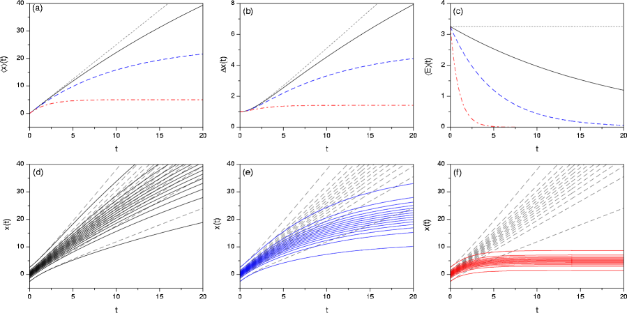
Figure 1: Top: Average position (a), dispersion (b), and energy (c) for a Gaussian wave packet in free space affected by friction. Different values for the friction coefficient have been considered: $\gamma=0.025$ (black solid line), $\gamma=0.1$ (blue dashed line), and $\gamma=0.5$ (red dash-dotted line). To compare with, the frictionless case ($\gamma=0$) has also been included and is denoted with the gray dotted line. The value of the other parameters considered in these simulations were: $x_{0}=0$, $p_{0}=2.5$ ($E_{0}=3.25$), $\sigma_{0}=1$, $m=1$, and $\hbar=1$. Bottom: Bohmian trajectories associated with the three dissipative cases considered atop: (d) $\gamma=0.025$, (e) $\gamma=0.1$, and (f) $\gamma=0.5$. Again, to compare with, the trajectories for the frictionless case (with the same initial conditions) have also been included in each panel (gray dashed lines). The initial positions have been distributed according to the initial Gaussian probability density.

4.2 Motion under a linear potential

In the case of a linear potential, e.g., a gravitational or an electric field, the classical solutions are also readily available. Thus, if $V(x)=-max$ (with $a>0$, without loss of generality), we find

$$x_{t} = x_{0}+\frac{p_{0}}{m}\left(\frac{1-e^{-\gamma t}}{\gamma}\right)+a\left(\frac{\gamma t-1+e^{-\gamma t}}{\gamma^{2}}\right),$$ (39)

$$p_{t} = p_{0}e^{-\gamma t}+ma\left(\frac{1-e^{-\gamma t}}{\gamma}\right),$$ (40)

while $\alpha_{t}$ and $\gamma_{t}$ keep the same functional form as in the free damped case (although $\mathcal{L}_{t}$ varies for the latter due to the presence of a nonzero potential function), because only second-order derivatives influence the evolution of these parameters (through $V^{\prime\prime}_{t}$, as seen in (21)).

Again in this case, the frictionless limit $\gamma\to 0$ leads us to the well-known expressions for uniform accelerated motion, with $x_{t}=x_{0}+(p_{0}/m)t+(a/2)t^{2}$ and $p_{t}=p_{0}+mat$. The wave packet also approaches the expression corresponding to the solution to ramp-like potentials [43], equal to (33), except for the different functional form of $E_{t}$ ($E_{t}=p_{0}^{2}/2m-max_{0}$) and an extra term coming from the classical action. Regarding the long-time limit for finite friction (i.e., for $t\gg\gamma^{-1}$), we find that while the wave packet freezes its spreading, as in the previous example, it still keeps moving due to the constant limit momentum, $p_{\infty}=ma/\gamma$. Accordingly, the centroid of the wave-packet displays a uniform motion described by

$$x_{t\to\infty}=x_{0}+\frac{p_{0}}{m\gamma}-\frac{a}{\gamma^{2}}+\frac{a}{\gamma}\ t.$$ (41)

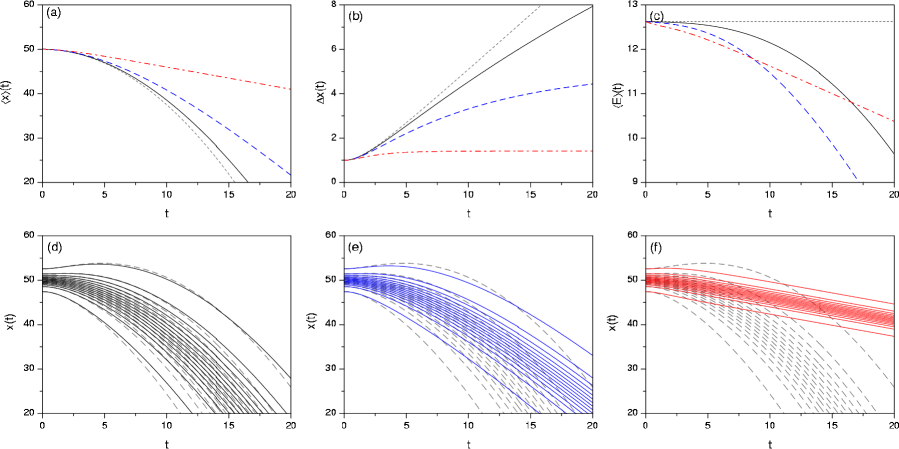
Figure 2: Top: Average position (a), dispersion (b), and energy (c) for a Gaussian wave packet subject to the action of a linear potential, with $a=0.25$, and affected by friction. Different values for the friction coefficient have been considered: $\gamma=0.025$ (black solid line), $\gamma=0.1$ (blue dashed line), and $\gamma=0.5$ (red dash-dotted line). To compare with, the frictionless case ($\gamma=0$) has also been included and is denoted with the gray dotted line. The value of the other parameters considered in these simulations were: $x_{0}=50$, $p_{0}=0$ ($E_{0}=12.625$), $\sigma_{0}=1$, $m=1$, and $\hbar=1$. Bottom: Bohmian trajectories associated with the three dissipative cases considered atop: (d) $\gamma=0.025$, (e) $\gamma=0.1$, and (f) $\gamma=0.5$. Again, to compare with, the trajectories for the frictionless case have also been included in each panel (gray dashed lines). The initial positions have been distributed according to the initial Gaussian probability density.

These aspects are illustrated in the top panels of Fig. 2, where the average position (a), dispersion (b), and energy (c) are plotted for the same values considered in the previous section, and considering $a=0.25$. Moreover, the frictionless homologous curves have also been included for comparison (gray dotted line). As it can be noticed, as $\gamma$ increases, the transition from a uniformly accelerated motion, displayed by the wave-packet centroid (see Fig. 2(a)), to a uniform rectilinear one, as a consequence of the damping, becomes more apparent. The evolution towards this type of limit motion, however, does not affect the width of the wave packet differently from the case analyzed in the previous section, but it appears very clearly in the average energy, particularly at large values of $\gamma$. As it can be readily shown, the expression for the average energy is given by

$$\bar{E}=\frac{p_{0}^{2}}{2m}\ e^{-2\gamma t}-max_{0}-p_{0}a\gamma\left(\frac{1-e^{-\gamma t}}{\gamma}\right)^{2}+\frac{ma^{2}}{2}\left(\frac{3-2\gamma t-4e^{-\gamma t}+e^{-2\gamma t}}{\gamma^{2}}\right)+\frac{\hbar^{2}}{8m\sigma_{0}^{2}}\ e^{-2\gamma t},$$ (42)

In the limit $\gamma t\gg 1$, this expression approaches

$$\bar{E}=-max_{0}-\frac{p_{0}a}{\gamma}+\frac{ma^{2}}{2\gamma^{2}}\left(3-2\gamma t\right).$$ (43)

The linear regime typical of the limit motion can be inferred for the lower values of $\gamma$. However, this effect is more remarkable for larger $\gamma$, since the transient exponentials vanish quickly and the energy immediately manifests its linear dependence on time. Unlike the example of the free wave packet, here the energy does not approach zero asymptotically, but it continues decreasing below it as the wave packet slides downhill, unless some additional constraint is imposed in the dynamics to avoiding this situation. This is precisely the case of confining potential functions displaying local minima, such as the harmonic oscillator, which will be studied in the next section (for similar behaviors in non-harmonic systems, for example, see [44]). Nevertheless, although there is no suppression of the motion, we can still observe spatial localization.

To some extent the behavior displayed by the wave packet under the action of a linear potential is similar, asymptotically, to reach a classical-like regime. This can be better understood by inspecting the associated Bohmian trajectories. These trajectories are plotted in the lower panels of Fig. 2, from (d) to (e) for increasing values of $\gamma$. It is interesting that, because $\alpha_{t}$ does not depend on the potential function, the functional form displayed by the trajectories is exactly the same as in the free case, except for the fact that these trajectories contain information about the acceleration undergone by the centroid (this information is transmitted through $x_{t}$). Now, once the transients have vanished, all these trajectories evolve parallel one another, just like classical trajectories under similar circumstances (i.e., in this limit case).

4.3 Motion in a damped harmonic oscillator

Let us consider now the case of a harmonic oscillator potential, $V(x)=m\omega_{0}^{2}x^{2}/2$. In a frictionless situation, this system is characterized by a series of eigenstates

$$\Phi_{n}(x,t)=N_{n}e^{-(m\omega_{0}/2\hbar)x^{2}-i(n+1/2)\omega_{0}t}H_{n}(\sqrt{m\omega_{0}/\hbar}x),$$ (44)

with eigenenergy $E_{n}=(n+1/2)\hbar\omega_{0}$, and where $H_{n}$ is the Hermite polynomial of degree $n$ and $N_{n}=(1/\sqrt{2^{n}n!})(\pi\hbar/m\omega_{0})^{-1/4}$ is the normalization constant. These eigenvalues can be obtained by employing the same method used above to derive the analytical expression of the time-evolved wave packets [37]. So, similarly, it can be used to determine the dissipative counterpart of (44),

$$\Phi_{n}(x,t) = N_{n}e^{-(m\Omega/2\hbar)(1+i\gamma/2\Omega)e^{\gamma t}x^{2}-i(n+1/2)\Omega t+\gamma t/4}H_{n}(\sqrt{m\Omega/\hbar}e^{\gamma t/2}x)$$ (45)

$$= N_{n}e^{-(m\Omega/2\hbar)e^{\gamma t}x^{2}-i(n+1/2)\Omega t-i(m\gamma/4\hbar)e^{\gamma t}x^{2}+\gamma t/4}H_{n}(\sqrt{m\Omega/\hbar}e^{\gamma t/2}x).$$

However, contrary to (44), Eq. (45) describes a quasi-stationary state, i.e., states that, at each time, are eigenstates of the dissipative Schrödinger equation, but that eventually collapse to zero, as formerly shown by Vandyck [31]. Of course, these states are only defined for $\omega_{0}>\gamma/2$, as it will be explained later on.

Concerning the associated Bohmian trajectories, from (45), we obtain

$$\dot{x}=-\frac{\gamma}{2}\ x,$$ (46)

which after integration renders

$$x(t)=x(0)e^{-\gamma t/2}.$$ (47)

That is, regardless of the eigenstate considered, any trajectory falls down to the bottom of the potential at the same rate, $\gamma/2$, and therefore merging asymptotically at $x=0$. The reason for such a behavior is that the model is fully dissipative and there is no possibility for a feedback with an environment, as happens when a Brownian-like motion is assumed. In this latter case, the stochastic fluctuations accounting for the feedback with a surrounding medium would be enough to sustain a dynamical regime (even if stationary) and avoid its full collapse.

The previous case was already investigated by Vandyck [31] and in order to gain insight on it, now we are going to consider the case of a coherent (or minimum uncertainty) Gaussian wave packet initially centered around the turning point $x=x_{0}$ ($p_{0}=0$). At any subsequent time, this wave packet is described by

$$\Psi(x,t)=\left(\frac{1}{2\pi\sigma_{0}^{2}}\right)^{1/4}e^{-(x-x_{t})^{2}/4\sigma_{0}^{2}+ip_{t}(x-x_{t})/\hbar-i\omega_{0}t/2+ip_{t}x_{t}/\hbar},$$ (48)

with $x_{t}=x_{0}\cos\omega_{0}t$ and $p_{t}=-m\omega_{0}x_{0}\sin\omega_{0}t$. The corresponding probability density reads as

$$|\Psi(x,t)|^{2}=\frac{1}{\sqrt{2\pi\sigma_{0}^{2}}}\ e^{-[x-x_{0}\cos(\omega_{0}t)]^{2}/2\sigma_{0}^{2}},$$ (49)

where $\sigma_{0}^{2}=\hbar/(2m\omega_{0})$ for the wave packet (48) to be coherent (otherwise the wave packet will keep its Gaussian shape, but it will display an oscillating variation of its width or “breathing” as it moves back and forth between the two turning points). The corresponding quantum action is

$$S(x,t)=-\frac{1}{2}\ \hbar\omega_{0}t-\frac{m\omega_{0}}{4}\left[4xx_{0}\sin(\omega_{0}t)-x_{0}^{2}\sin(2\omega_{0}t)\right],$$ (50)

which leads to Bohmian trajectories oscillating with the same frequency as $x_{t}$, but around their initial position, i.e.,

$$x(t)=[x(0)-x_{0}]+x_{0}\cos(\omega_{0}t).$$ (51)

As also happens in classical mechanics, in order to proceed analytically in the dissipative case, it is important to distinguish three cases depending on whether $\omega_{0}$ is larger than, equal to or smaller than $\gamma/2$, i.e., if we have underdamped oscillatory motion, critically damped motion, or overdamped motion, respectively. These situations lead to the following solutions for the centroidal trajectory:

$$\omega_{0}>\gamma/2 \Longrightarrow \left\{\begin{array}[]{rcl}x_{t}&=&\displaystyle\left(\frac{\omega_{0}}{\Omega}\right)x_{0}e^{-\gamma t/2}\cos(\Omega t-\varphi)\\ p_{t}&=&\displaystyle-m\left(\frac{\omega_{0}^{2}}{\Omega}\right)x_{0}e^{-\gamma t/2}\sin\Omega t\end{array}\right.,$$ (54)

$$\omega_{0}=\gamma/2 \Longrightarrow \left\{\begin{array}[]{rcl}x_{t}&=&\displaystyle x_{0}\left(1+\frac{\gamma}{2}\ t\right)e^{-\gamma t/2}\\ p_{t}&=&\displaystyle-mx_{0}\left(\frac{\gamma}{2}\right)^{2}e^{-\gamma t/2}\end{array}\right.,$$ (57)

$$\omega_{0}<\gamma/2 \Longrightarrow \left\{\begin{array}[]{rcl}x_{t}&=&\displaystyle\left(\frac{\omega_{0}}{\Gamma}\right)x_{0}e^{-\gamma t/2}\cosh(\Gamma t+\phi)\\ p_{t}&=&\displaystyle-m\left(\frac{\omega_{0}^{2}}{\Gamma}\right)x_{0}e^{-\gamma t/2}\sinh\Gamma t\end{array}\right.,$$ (60)

where $\Omega=\sqrt{\omega_{0}^{2}-(\gamma/2)^{2}}$, $\varphi=(\tan)^{-1}(\gamma/2\Omega)$, $\Gamma=i\Omega$, and $\phi=(\tanh)^{-1}(\gamma/2\Gamma)$. The relationship between $\omega_{0}$ and $\gamma$ also influences the calculation of $\alpha_{t}$ and $f_{t}$. In the case of $\alpha_{t}$, the equation of motion to be solved is

$$\dot{\alpha}_{t}=-\frac{2\alpha_{t}^{2}}{m}\ e^{-\gamma t}-\frac{1}{2}\ m\omega_{0}^{2}e^{\gamma t},$$ (61)

which can be conveniently rearranged by introducing the change $\alpha_{t}=g_{t}e^{\gamma t}$. This leads to the equation of motion

$$\dot{g}_{t}=-\frac{2}{m}\ \left[g_{t}^{2}+\frac{m\gamma}{2}\ g_{t}+\left(\frac{m\omega_{0}}{2}\right)^{2}\right]=-\frac{2}{m}\ (g_{t}-g_{+})(g_{t}-g_{-}),$$ (62)

which does not contain exponential terms, and where

$$g_{\pm}=\frac{m}{2}\left[-\frac{\gamma}{2}\pm\sqrt{\left(\frac{\gamma}{2}\right)^{2}-\omega_{0}^{2}}\right].$$ (63)

From the latter expression, it is now clear how the three cases of damped motion also rule the behavior of $\alpha_{t}$, although there are some physical subtleties to take into account. If $\omega_{0}\neq\gamma/2$, the general solution for $g_{t}$ reads as

$$g_{t}=\frac{g_{+}(g_{0}-g_{-})e^{\beta t}-g_{-}(g_{0}-g_{+})e^{-\beta t}}{(g_{0}-g_{-})e^{\beta t}-(g_{0}-g_{+})e^{-\beta t}},$$ (64)

where $\beta=\sqrt{(\gamma/2)^{2}-\omega_{0}^{2}}$ and $g_{0}$ is the initial condition. Otherwise, if $\omega_{0}=\gamma/2$ (critically damped motion), we have $g_{+}=g_{-}$ and Eq. (62) becomes

$$\dot{g}_{t}=-\frac{2}{m}\ (g_{t}-g_{s})^{2},$$ (65)

with $g_{s}=-m\gamma/4$. The integration in time of this equation of motion yields

$$g_{t}=g_{s}+\frac{g_{0}-g_{s}}{1+(g_{0}-g_{s})(2t/m)}.$$ (66)

If we now assume that our initial wave packet is (48) and consider the initial condition $g_{0}=\alpha_{0}=\alpha_{t}=im\omega_{0}/2$, then $g_{t}$ becomes an oscillatory function of time for $\omega_{0}>\gamma/2$, since $\beta=i\Omega$. Otherwise, it becomes a monotonically decreasing function of time, with the asymptotic limits $g_{\infty}=g_{s}$ if $\omega_{0}=\gamma/2$, or $g_{\infty}=g_{+}$ (with $\beta=\Gamma$) if $\omega_{0}<\gamma/2$.

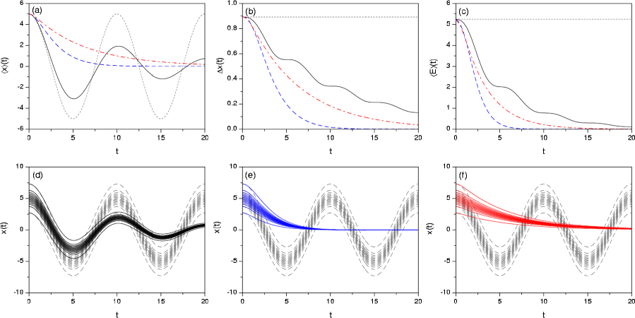
Figure 3: Top: Average position (a), dispersion (b), and energy (c) for a coherent wave packet in a harmonic oscillator, with $\omega_{0}=2\pi/\tau_{0}\approx 0.628$ ($\tau_{0}=10$), affected by friction. Values for the friction coefficient illustrative of the three regimes have been considered: $\gamma=0.3\omega_{0}$ (black solid line), $\gamma=2\omega_{0}$ (blue dashed line), and $\gamma=4\omega_{0}$ (red dash-dotted line). To compare with, the frictionless case ($\gamma=0$) has also been included and is denoted with the gray dotted line. The values of the other parameters considered in these simulations were: $x_{0}=5$, $p_{0}=0$ ($E_{0}\approx 5.249$), $\sigma_{0}=\sqrt{\hbar/2m\omega_{0}}\approx 0.892$, $m=1$, and $\hbar=1$. Bottom: Bohmian trajectories associated with the three dissipative cases considered atop: (d) $\gamma=0.3\omega_{0}$, (e) $\gamma=2\omega_{0}$, and (f) $\gamma=4\omega_{0}$. Again, to compare with, the trajectories for the frictionless case have also been included in each panel (gray dashed lines). The initial positions have been distributed according to the initial Gaussian probability density.

In the top panels of Fig. 3, we show the average position (a), dispersion (b), and energy (c) for a wave function with the initial form of the coherent state (48) in the three dissipative regimes, with: $\gamma=0.3\omega_{0}$ (black solid line), $\gamma=2\omega_{0}$ (blue dashed line), and $\gamma=4\omega_{0}$ (red dash-dotted line). To compare with, the corresponding frictionless values have also been included in each panel (gray dotted lines). In the lower panels, we have included the corresponding Bohmian trajectories, which effectively follow the dissipative flow, falling down to the bottom of the well and merging into the centroidal one.

We are not going to enter into more details here on the particular analytical expressions for the quantities displayed in Fig. 3, as well as those for the corresponding Bohmian trajectories. Nonetheless, they bring in an interesting question. As seen in Fig. 3(b), the decay of the dispersion or width of the wave packet under underdamped conditions does not follow a monotonic exponential-like decay, but displays an oscillating behavior. Moreover, in the frictionless case, we saw that the initial condition $\alpha_{0}=im\omega_{0}/2$ led to a time-independent width of the wave packet. An interesting analog also arises in the dissipative case if we change the initial condition. Notice in Eq. (64) that $g_{t}$ remains constant with time if we assume that $g_{0}$ is equal to either $g_{+}$ or $g_{-}$, which can be inferred either from (64) or also directly from (62) by setting $\dot{g}_{t}=0$. This means $\alpha_{t}=g_{+}e^{\gamma t}$, if $g_{0}=g_{+}$, or $\alpha_{t}=g_{-}e^{\gamma t}$, if $g_{0}=g_{-}$. In order to choose the appropriate solution, we consider the fact that in the limit $\gamma\to 0$ the chosen solution has to approach the non-dissipative value, i.e., $\alpha_{t}\to im\omega_{0}/2$, which only happens if $g_{0}=g_{+}$. Therefore, we have that

$$\alpha_{t}=\frac{im\Omega}{2}\left(1+\frac{i\gamma}{2\Omega}\right)e^{\gamma t}.$$ (67)

Notice that in the limit of vanishing friction, this value approaches the frictionless one mentioned above. More importantly, $\alpha_{t}$ has a real and an imaginary part, and therefore the wave function will be properly normalized. This can be readily seen by integrating the equation of motion for $f_{t}$, which leads to

$$f_{t}=\frac{i\hbar}{4}\ \ln\left(\frac{\pi\hbar}{m\Omega}\right)-\frac{\hbar\Omega}{2}\left(1+\frac{i\gamma}{2\Omega}\right)t+\mathcal{S}_{{\rm cl},t}.$$ (68)

Substituting all these parameters in the functional expression for the wave function, it reads as

$$\Psi(x,t) = \left(\frac{\pi\hbar}{2{\rm Im}\{\alpha_{0}\}}\right)^{1/4}e^{-(m\Omega/2\hbar)(1+i\gamma/2\Omega)e^{\gamma t}(x-x_{t})^{2}+ip_{t}(x-x_{t})/\hbar-i\Omega t(1+i\gamma/2\Omega)/2+i\mathcal{S}_{{\rm cl},t}/\hbar},$$ (69)

$$= \left(\frac{1}{2\pi\sigma_{t}^{2}}\right)^{1/4}e^{-(x-x_{t})^{2}/4\sigma_{t}^{2}+ip_{t}(x-x_{t})/\hbar-i\Omega t/2-(im\gamma/4\hbar)e^{\gamma t}(x-x_{t})^{2}+i\mathcal{S}_{{\rm cl},t}/\hbar},$$

with the width being $\sigma_{t}=e^{-\gamma t/2}\sqrt{\hbar/2m\Omega}$. As it can be noticed, the first three arguments in the exponential of (69) are identical to those in (48), but replacing $\omega_{0}$ by $\Omega$. The wave function is properly normalized, but its width decreases exponentially with time, according to

$$\Delta x=\sigma_{t}e^{-2\gamma t}.$$ (70)

Thus, it eventually collapses over the center of the harmonic well as the whole wave packet follows the motion of a damped harmonic oscillator. Along this transit, the system energy is also exponentially lost, according to

$$\bar{E}=\frac{1}{2}\ m\omega_{0}^{2}x_{0}^{2}\left(\frac{\omega_{0}}{\Omega}\right)^{2}\left[1-\frac{\gamma}{2\omega_{0}}\ \sin(2\Omega t-\varphi)\right]e^{-\gamma t}+\frac{1}{2}\ \omega_{0}\hbar\left(\frac{\omega_{0}}{\Omega}\right)e^{-\gamma t}.$$ (71)

It is worth stressing that for underdamped conditions, $\alpha_{t}$, given by (67), is a complex function, which makes the wave function (69) to display a vanishing Gaussian shape plus a phase factor as the system oscillates, as seen in (69). Critically damped and overdamped conditions imply that the motion amplitude of the system exhibits a monotonic decrease to zero, with no oscillations. In the present context, where we are seeking for solutions such that $\dot{g}_{t}=0$, this now translates into a rather puzzling quantum behavior. In order to analyze it, let us start from the overdamped condition, $\omega_{0}<\gamma/2$. Equation (64) is still valid, although we have $g_{\pm}=\pm(m\Gamma/2)(1\mp\gamma/2\Gamma)$. Between these two solutions, we choose $g_{+}$, because it is consistent with (67) and also because it corresponds to the long-time limit of $g_{t}$ in this case (i.e., for $\beta=\Gamma$). Accordingly, the spreading factor will read as

$$\alpha_{t}=\frac{m\Gamma}{2}\left(1-\frac{\gamma}{2\Gamma}\right)e^{\gamma t},$$ (72)

which is a pure real function. From it,

$$f_{t}=f_{0}+\frac{i\hbar\Gamma}{2}\left(1-\frac{\gamma}{2\Gamma}\right)t+\mathcal{S}_{{\rm cl},t},$$ (73)

where $f_{0}$ is now left as a free parameter, although its imaginary part has to be such that the initial plane wave is still normalized and validates the working hypothesis regarding the expectation values of the position and momentum. Notice that in this case, the corresponding wave function reads as

$$\Psi(x,t)=e^{-(im\Gamma/2\hbar)(1+\gamma/2\Gamma)e^{\gamma t}(x-x_{t})^{2}+ip_{t}(x-x_{t})/\hbar+\Gamma t(1+\gamma/2\Gamma)/2+if_{0}+i\mathcal{S}_{{\rm cl},t}/\hbar},$$ (74)

which is a pure phase factor multiplied by a diverging time-dependent exponential. It is interesting, though, that although the wave function itself diverges, the associated Bohmian trajectories are well-defined and approach asymptotically the classical overdamped centroid, $x_{t}$ (see below).

Regarding the critically damped situation, if we consider here the initial value $g_{0}=g_{s}$, the stationary solution is $g_{t}=g_{s}=-m\gamma/4$, and therefore

$$\alpha_{t}=-\frac{m\gamma}{4}\ e^{\gamma t}.$$ (75)

As it can be seen, this value of $\alpha_{t}$ allows us to connect smoothly those two previously obtained in underdamped and overdamped cases as the friction $\gamma$ is gradually increased.

In spite of the type of motion displayed in each one of the regimes discussed above, the Bohmian equation of motion for the trajectories can be recast in the same form for all of them,

$$\frac{d(x-x_{t})}{x-x_{t}}=-\frac{\bar{\gamma}}{2}\ dt,$$ (76)

where $\bar{\gamma}=\gamma$ for underdamped and critically damped motions, and $\bar{\gamma}=\gamma-2\Gamma$ for overdamped motions. As it can be noticed, this equation looks exactly the same as Eq. (46) for the eigenstates, although replacing $x$ by $x-x_{t}$. Thus, the solutions,

$$x(t)=x_{t}+[x(0)-x_{0}]e^{-\bar{\gamma}t/2},$$ (77)

are also very similar. In the case of Eq. (47), since the associated wave function is a quasi-eigenstate, the trajectory approaches asymptotically the origin or, in other words, it falls down to the bottom of the well. In the case of Eq. (77), and differently to what we have seen in the two previous sections, any trajectory will eventually coalesce with the centroidal one. This is an interesting case where the Bohmian non-crossing rule seems to be violated. However, we have to keep in mind that we are describing an effective dissipative dynamics, which only models phenomenologically the system behavior, but now its true interaction with the environment causing such an effect. Actually, the evolution of the trajectories is in compliance with the shrinking undergone by the wave function in the damped oscillatory regime and its evanescent nature in the overdamped regime. These trajectories, described generically by Eq. (77), have the following explicit functional form

$$x(t)=\left\{\begin{array}[]{lcc}\left\{\displaystyle[x(0)-x_{0}]+x_{0}\left(\frac{\omega_{0}}{\Omega}\right)\cos(\Omega t-\varphi)\right\}e^{-\gamma t/2},&&\omega_{0}>\gamma/2\\ \left\{\displaystyle[x(0)-x_{0}]+x_{0}\left(1+\frac{\gamma t}{2}\right)\right\}e^{-\gamma t/2},&&\omega_{0}=\gamma/2\\ \left\{\displaystyle[x(0)-x_{0}]e^{\Gamma t}+x_{0}\left(\frac{\omega_{0}}{\Gamma}\right)\cosh(\Gamma t+\phi)\right\}e^{-(\gamma-2\Gamma)t/2},&&\omega_{0}<\gamma/2\end{array}\right.,$$ (78)

where the first expression looks very similar to that for the unperturbed harmonic oscillator, with the exception of the overall exponentially decaying factor and the dephasing in the cosine function.

4.4 Interference dynamics

Now, consider a problem involving wave-packet interference, for which a general solution can be expressed as a coherent superposition [40],

$$\Psi=\mathcal{N}(\Psi_{1}+\Psi_{2}),$$ (79)

with $\mathcal{N}$ being the overall norm factor (it is assumed that each Gaussian wave packet, given by (33), is normalized). As it can be shown, the associated Bohmian equation of motion reads as

$$\dot{x} = \frac{\rho_{1}}{\rho}\ \dot{x}_{1}+\frac{\rho_{2}}{\rho}\ \dot{x}_{2}+\frac{\hbar}{2mi\rho}\left(\Psi_{1}^{*}\partial_{x}\Psi_{2}-\Psi_{2}\partial_{x}\Psi_{1}^{*}\right)e^{-\gamma t}+\frac{\hbar e^{-\gamma t}}{2mi\rho}\left(\Psi_{2}^{*}\partial_{x}\Psi_{1}-\Psi_{1}\partial_{x}\Psi_{2}^{*}\right)e^{-\gamma t}$$ (80)

$$= \frac{\rho_{1}}{\rho}\left[\frac{p_{t,1}}{m}+\frac{2{\rm Re}\{\alpha_{t,1}\}}{m}\ (x-x_{t,1})\ e^{-\gamma t}\right]+\frac{\rho_{2}}{\rho}\left[\frac{p_{t,2}}{m}+\frac{2{\rm Re}\{\alpha_{t,2}\}}{m}\ (x-x_{t,2})\ e^{-\gamma t}\right]$$

$$+2\cos\xi_{12}\ \frac{\sqrt{\rho_{1}\rho_{2}}}{\rho}\left[\frac{p_{t,1}+p_{t,2}}{2m}+\left[\frac{{\rm Re}\{\alpha_{t,1}\}(x-x_{t,1})+{\rm Re}\{\alpha_{t,2}\}(x-x_{t,2})}{m}\right]e^{-\gamma t}\right]$$

$$-2\sin\xi_{12}\ \frac{\sqrt{\rho_{1}\rho_{2}}}{\rho}\left[\frac{{\rm Im}\{\alpha_{t,1}\}(x-x_{t,1})-{\rm Im}\{\alpha_{t,2}\}(x-x_{t,2})}{m}\right]e^{-\gamma t},$$

where $\dot{x}_{i}$ refers to the equation of motion for the $i$th wave packet and $\xi_{12}=(S_{1}-S_{2})/\hbar$, being $\rho_{i}$ and $S_{i}$ the probability density and real phase associated with the $i$th wave packet when it is expressed in polar form. As it can be noticed, this expression simply reflects the sum of two separate fluxes, each one associated with one wave packet, plus another one coming from their interference.

Depending on the value given to the parameters of each wave packet, one can generate different dynamics. For example, if they have the same width ($\alpha_{t,1}=\alpha_{t,2}=\alpha_{t}$) and are located at symmetric positions with respect to $x=0$ ($x_{t,1}=x_{0}=-x_{t,2}$), then (80) simplifies to

$$\dot{x} = \frac{\rho_{1}}{\rho}\left[\frac{p_{t,1}}{m}+\frac{2{\rm Re}\{\alpha_{t}\}}{m}\ (x-x_{0})e^{-\gamma t}\right]+\frac{\rho_{2}}{\rho}\left[\frac{p_{t,2}}{m}+\frac{2{\rm Re}\{\alpha_{t}\}}{m}\ (x+x_{0})e^{-\gamma t}\right]$$ (81)

$$+2\cos\xi_{12}\ \frac{\sqrt{\rho_{1}\rho_{2}}}{\rho}\left[\frac{p_{t,1}+p_{t,2}}{2m}+\frac{2{\rm Re}\{\alpha_{t}\}}{m}\ xe^{-\gamma t}\right]+2\sin\xi_{12}\ \frac{\sqrt{\rho_{1}\rho_{2}}}{\rho}\left[\frac{2{\rm Im}\{\alpha_{t}\}}{m}\ x_{0}e^{-\gamma t}\right].$$

Thus, consider the case of two interfering coherent wave packets in free space. This situation, for example, mimics the situation of a two slit experiment when each wave packet is associated with one of the diffracted beams. In such a case, if the longitudinal propagation (parallel to the diffractive screen) is slower than the perpendicular one (in the direction of the diffracted beam), both motions can be decoupled and treated as two independent one-dimensional propagations, one longitudinal and the other translational, the latter being well accounted for by a plane wave. Now, if one assumes that $p_{0,1}=p_{0,2}=0$, i.e., there is no translational motion along the longitudinal direction, but only spreading of the two wave packets [40], the above expression (81) will read as

$$\dot{x} = \frac{\rho_{1}}{\rho}\left[\frac{2{\rm Re}\{\alpha_{t}\}}{m}\ (x-x_{0})\ e^{-\gamma t}\right]+\frac{\rho_{2}}{\rho}\left[\frac{2{\rm Re}\{\alpha_{t}\}}{m}\ (x+x_{0})\ e^{-\gamma t}\right]$$ (82)

$$+2\cos\xi_{12}\ \frac{\sqrt{\rho_{1}\rho_{2}}}{\rho}\left[\frac{2{\rm Re}\{\alpha_{t}\}}{m}\ xe^{-\gamma t}\right]+2\sin\xi_{12}\ \frac{\sqrt{\rho_{1}\rho_{2}}}{\rho}\left[\frac{2{\rm Im}\{\alpha_{t}\}}{m}\ x_{0}e^{-\gamma t}\right].$$

Results after integration of this equation of motion for different values of $\gamma$ (the same values as in the case of the free wave packet treated above) can be seen in Fig. 4. As it can be seen through the sets of trajectories selected, the friction of the medium leads to the localization of the two wave packets by gradually “freezing” them rather than by annihilating the coherence between them due to the interaction with an environment, as happens with [29, 45]. In other words, the reason why interference is not observed in a quantum viscid medium is because the wave packets cannot be seen each other, rather than because the destruction (over time) of their mutual coherence.

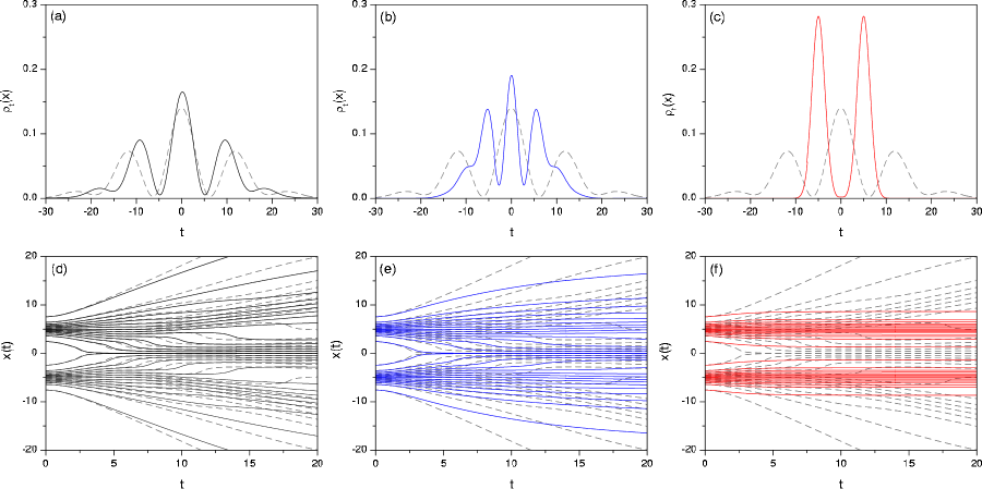
Figure 4: Top: Final probability density (at $t=20$) for a coherent superposition of two Gaussian wave packets in free space affected by friction. The same friction values as in Fig. 1 have been considered: (a) $\gamma=0.025$ (black solid line), (b) $\gamma=0.1$ (blue solid line), and (c) $\gamma=0.5$ (red solid line). To compare with, the frictionless case ($\gamma=0$) has also been included in each panel (gray dashed line). The value of the other parameters considered in these simulations were: $x_{0,1}=5=-x_{0,2}$, $p_{0,1}=p_{0,2}=0$ ($E_{0}=3.25$), $\sigma_{0,1}=\sigma_{0,2}=1$, $m=1$, and $\hbar=1$. Bottom: Bohmian trajectories associated with the three dissipative cases considered atop: (d) $\gamma=0.025$, (e) $\gamma=0.1$, and (f) $\gamma=0.5$. Again, to compare with, the trajectories for the frictionless case (with the same initial conditions) have also been included in each panel (gray dashed lines). The initial positions have been distributed according to the initial Gaussian probability density.

Another situation of interest is when the two wave packets are inside a harmonic oscillator, each one launched from an opposite turning point (i.e., again $x_{0,1}=x_{0}=-x_{0,2}$). In this case, $x_{t,1}=-x_{t,2}$ and $p_{t,1}=-p_{t,2}$, so the general form of equation of motion (82) remains still valid, although also keeping the two momentum terms that appear in the first line of (81). This dissipative dynamics is illustrated in Fig. 5 for the same cases treated above for the harmonic oscillator. As it can be seen, because of the presence of the oscillator, both wave packets approach the center of the well, but without ever crossing it: in the underdamped case a series of bounces are observed until the trajectories merge into the single asymptotic one at $x=0$, while for the critically damped and overdamped cases the two sets of trajectories gradually merge into this asymptotic one. Again here we find an example of spatial localization, although it is different from the free case seen above, since the final wave function becomes a $\delta$-like function regardless of where the trajectories came from, whether from one turning point or the other.

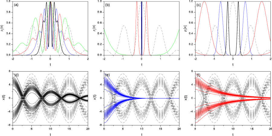
Figure 5: Top: Probability density at different times for a coherent superposition of two Gaussian wave packets (coherent states) in a harmonic oscillator, with $\omega_{0}=2\pi/\tau_{0}\approx 0.628$ ($\tau_{0}=10$), affected by friction. The same friction values as in Fig. 3 have been considered: (a) $\gamma=0.3\omega_{0}$, (b) $\gamma=2\omega_{0}$, and (c) $\gamma=4\omega_{0}$. In each panel, in order to better appreciate the damping effects, the probability density at times of maximal interference in the frictionless case is shown: $t=\tau_{0}/2$ (green solid line), $t=3\tau_{0}/2$ (red solid line), $t=5\tau_{0}/2$ (blue solid line), and $t=7\tau_{0}/2$ (black thick solid line); to compare with, the frictionless ($\gamma=0$) probability density at these times has also been included in each panel (gray dashed line). Moreover, to better appreciate the effect of friction with time, the maximum for all probability densities has been re-scaled to 1. Bottom: Bohmian trajectories associated with the three dissipative cases considered atop: (d) $\gamma=0.3\omega_{0}$, (e) $\gamma=2\omega_{0}$, and (f) $\gamma=4\omega_{0}$. Again, to compare with, the trajectories for the frictionless case (with the same initial conditions) have also been included in each panel (gray dashed lines). The initial positions have been distributed according to the initial Gaussian probability density.

5 Concluding remarks

The approach presented here to deal with dissipation in quantum viscid media is based on Bohmian mechanics. However, an even more direct link can be established with the hydrodynamic reformulation of Schrödinger’s wave mechanics proposed in 1926 by Madelung [27]. Accordingly, the evolution of a quantum system can be connected to that of an ideal (quantum) fluid by means of a simple nonlinear transformation, which goes from the wave function to two real fields, namely the probability density and the phase field (or, to make the analogy more apparent, the quantum current density). This work would then go a step beyond by assuming the medium is not ideal, but viscid. To some extent, the introduction of a friction makes the approach to somehow resemble Bell’s beables interpretation, particularly as further developed by Vink [46] and Lorenzen et al. [13]. Actually, the latter also considered friction as a means to interpret and understand phenomena such as dissipation, decoherence, or the quantum-to-classical transition in quantum systems.

Now, the problem posed by the Caldirola-Kanai model analyzed here is that the standard quantum uncertainty relations are violated. Alternative nonlinear models have been proposed in the literature to overcome this inconvenience, such as Kostin’s model [26], which includes in the Schrödinger equation a friction term proportional to the phase of the wave function (related, as seen above, to the Bohmian momentum). Because of this term, although the quantum system displays a similar damping to the one observed here, the width of the wave function does not collapse to zero in the case of the harmonic oscillator, for example, thus preserving the uncertainty relations. More importantly, this model has been recently used by Garashchuk and coworkers [44] with the practical purpose of obtaining the ground state in arbitrary potential functions —an analogous result, starting from similar grounds, was previously found by Doebner and Goldin [47]. The difference between the effective dissipative Schrödinger equation found by the latter authors with respect to Eq. (9) arises from the way how it is obtained from the Langevin equation (1). While in our case this is done from a linear, but time-dependent Hamiltonian operator, in the case of these authors the Hamiltonian is time-independent, but nonlinear —an interesting discussion on these two procedures can be found in [8]. From a physical viewpoint, the role of this nonlinearity is equivalent to adding a noise on the right-hand side of Eq. (1) in order to avoid the collapse of the system or its localization. That is, it enables a kind of fluctuation-dissipation relation, although the corresponding nonlinear Schrödinger equation (Kostin’s equation) still describes one subsystem and, therefore, the associated Bohmian trajectories are reduced in the same sense as those here analyzed (we still have an incomplete view of the process).

Alternative and possible applications of this type of studies can be developed in several ways. First, it is well known that a quantum Brownian particle moving in a periodic potential, coupled to a dissipative environment and at zero temperature, undergoes a transition from an extended to a localized ground state as the friction is raised [48, 49]. We think our methodology could throw some new light on this aspect as well as when a harmonic oscillator is interacting with a one-dimensional massless scalar field [50]. Second, when considering the lowest frequency motion or frustrated translational motion of adsorbates on corrugated surfaces [25]. In this problem, such a motion can be similarly seen as that described by a damped harmonic oscillator. It is true that a certain feedback between the thermal bath due to the presence of the surface and the quasi harmonic oscillator cannot be neglected. However, if the surface temperature is really low, the corresponding dynamics has to be closer to a pure dissipative dynamics as considered in this work. Third, within the same context, the diffusion of adsorbates on flat surfaces implies a free propagation of wave packets in the presence of friction. Again, the surface temperature is supposed to be low enough in order to highlight the role of the dissipation. In a flat surface, the collision between two adsorbates could also be described by the interference dynamics in presence of a thermal bath or surface. In this sense, a new friction mechanism could be added which is the so-called collisional friction [25]. And fourth, our study could be easily extended to gas phase molecular processes where the interaction among different molecules or atoms due to a high pressure could be replaced by such a friction mechanism. It should be then easily analyzed, for example, the broadening of spectral lines in this collisional regime.

References

- Weiss [1999] U. Weiss, Quantum Dissipative Systems, World Scientific, Singapore, 1999.
- Breuer and Petruccione [2002] H.-P. Breuer, F. Petruccione, The Theory of Open Quantum Systems, Oxford University Press, Oxford, 2002.
- Caldeira and Leggett [1983a] A. O. Caldeira, A. J. Leggett, Path integral approach to quantum Brownian motion, Physica A 121 (1983a) 587–616.
- Caldeira and Leggett [1983b] A. O. Caldeira, A. J. Leggett, Quantum tunneling in a dissipative system, Ann. Phys. (NY) 149 (1983b) 374–456.
- Caldirola [1941] P. Caldirola, Forze non conservative nella meccanica quantistica, Nuovo cim. 18 (1941) 393–400.
- Kanai [1948] E. Kanai, On the quantization of the dissipative systems, Prog. Theor. Phys. 3 (1948) 440–442.
- Kerner [1958] E. H. Kerner, Note on the forced and damped oscillator in quantum mechanics, Can. J. Phys. 36 (1958) 371–377.
- Schuch [1999] D. Schuch, Effective description of the dissipative interaction between simple model-systems and their environment, Int. J. Quantum. Chem. 72 (1999) 537–547.
- Majima and Suzuki [2011] H. Majima, A. Suzuki, Quantization and instability of the damped harmonic oscillator subject to a time-dependent force, Ann. Phys. 326 (2011) 3000–3012.
- Jannussis et al. [1980] A. Jannussis, P. Filipakis, T. Filipakis, Quantum friction in phase space, Physica 102A (1980) 561–567.
- Jannussis et al. [1979] A. D. Jannussis, G. N. Brodimas, A. Streclas, Propagator with friction in quantum mechanics, Phys. Lett. 74A (1979) 6–10.
- Khandekar and Lawande [1979] D. C. Khandekar, S. V. Lawande, Exact solution of a time-dependent quantal harmonic oscillator with damping and a perturbative force, J. Math. Phys. 20 (1979) 1870–1877.
- Lorenzen et al. [2009] F. Lorenzen, M. A. de Ponte, M. H. Y. Moussa, Extending Bell’s beables to encompass dissipation, decoherence, and the quantum-to-classical transition through quantum trajectories, Phys. Rev. A 80 (2009) 032101(1–8).
- Sun and Yu [1995] C.-P. Sun, L.-H. Yu, Exact dynamics of a quantum dissipative system in a constant external field, Phys. Rev. A 51 (1995) 1845–1853.
- Yu and Sun [1994] L.-H. Yu, C.-P. Sun, Evolution of the wave function in a dissipative system, Phys. Rev. A 49 (1994) 592–595.
- Schuch [1997] D. Schuch, Nonunitary connection between explicitly time-dependent and nonlinear approaches for the description of dissipative quantum systems, Phys. Rev. A 55 (1997) 935–940.
- Moshinsky and Schuch [2001] M. Moshinsky, D. Schuch, Diffraction in time with dissipation, J. Phys. A: Math. Gen. 34 (2001) 4217–4225.
- Moshinsky et al. [2001] M. Moshinsky, D. Schuch, A. Suárez-Moreno, Motion of wave packets with dissipation, Rev. Mex. Fís. 47 (2001) 7–10.
- Christoffel and Bowman [1981] K. M. Christoffel, J. M. Bowman, Quantum and classical dynamics of a coupled doble well oscillator, J. Chem. Phys. 74 (1981) 5057–5075.
- Guerra [1981] F. Guerra, Structural aspects of stochastic mechanics and stochastic field theory, Phys. Rep. 77 (1981) 263–312.
- Bateman [1931] H. Bateman, On dissipative systems and related variational principles, Phys. Rev. 38 (1931) 815–819.
- Brittin [1950] W. E. Brittin, A note on the quantization of dissipative systems, Phys. Rev. 77 (1950) 396–397.
- Senitzky [1960] I. R. Senitzky, Dissipation in quantum mechanics. The harmonic oscillator, Phys. Rev. 119 (1960) 670–679.
- Greenberger [1979] D. M. Greenberger, A critique of the major approaches to damping in quantum theory, J. Math. Phys. 20 (1979) 762–770.
- Sanz and Miret-Artés [2012a] A. S. Sanz, S. Miret-Artés, A Trajectory Description of Quantum Processes. I. Fundamentals, Springer, Berlin, 2012a.
- Kostin [1972] M. D. Kostin, On the Schrödinger-Langevin equation, J. Chem. Phys. 57 (1972) 3589–3591.
- Madelung [1926] E. Madelung, Quantentheorie in hydrodynamischer Form, Z. Phys. 40 (1926) 322–326.
- Cavalcanti [1998] R. M. Cavalcanti, Wave function of a Brownian particle, Phys. Rev. E 58 (1998) 6807–6809.
- Sanz and Borondo [2007] A. S. Sanz, F. Borondo, A quantum trajectory description of decoherence, Eur. Phys. J. D 44 (2007) 319–326.
- Sanz et al. [2012] A. S. Sanz, D. López-Durán, T. González-Lezana, Investigating transition state resonances in the time domain by means of Bohmian mechanics: The F+HD reaction, Chem. Phys. 399 (2012) 151–161.
- Vandyck [1994] M. A. Vandyck, On the damped harmonic oscillator in the de Broglie-Bohm hidden-variable theory, J. Phys. A: Math. Gen. 27 (1994) 1743–1750.
- Shojai and Shojai [2004] F. Shojai, A. Shojai, On the Bohmian quantum friction, PRAMANA 62 (2004) 803–814.
- Tilbi et al. [2007] A. Tilbi, T. Boudjedaa, M. Merad, L. Chetouani, The Kanai-Caldirola propagator in the de Broglie-Bohm theory, Phys. Scr. 75 (2007) 474–479.
- Hasse [1975] R. W. Hasse, On the quantum mechanical treatment of dissipative systems, J. Math. Phys. 16 (1975) 2005–2011.
- Razavy [2005] M. Razavy, Classical and Quantum Dissipative Systems, Imperial College Press, London, 2005.
- Kochan [2010] D. Kochan, Functional integral for non-Lagrangian systems, Phys. Rev. A 81 (2010) 022112(1–13).
- Heller [1975] E. J. Heller, Time-dependent approach to semiclassical dynamics, J. Chem. Phys. 62 (1975) 1544–1555.
- Tannor [2006] D. J. Tannor, Introduction to Quantum Mechanics: A Time-Dependent Perspective, University Science Books, Sausalito, CA, 2006.
- Sanz and Miret-Artés [2013] A. S. Sanz, S. Miret-Artés, A Trajectory Description of Quantum Processes. II. Applications, Springer, Berlin, 2014.
- Sanz and Miret-Artés [2008] A. S. Sanz, S. Miret-Artés, A trajectory-based understanding of quantum interference, J. Phys. A: Math. Theor. 41 (2008) 435303(1–23).
- Sanz and Miret-Artés [2012b] A. S. Sanz, S. Miret-Artés, Quantum phase analysis with quantum trajectories: A step towards the creation of a Bohmian thinking, Am. J. Phys. 80 (2012b) 525–533.
- Sanz and Miret-Artés [2007] A. S. Sanz, S. Miret-Artés, Aspects of nonlocality from a quantum trajectory perspective: A WKB approach to Bohmian mechanics, Chem. Phys. Lett. 445 (2007) 350–354.
- Sanz and Miret-Artés [2011] A. S. Sanz, S. Miret-Artés, Setting-up tunneling conditions by means of Bohmian mechanics, J. Phys. A: Math. Theor. 44 (2011) 485301(1–17).
- Garashchuk et al. [2013] S. Garashchuk, V. Dixit, B. Gu, J. Mazzuca, The Schrödinger equation with friction from the quantum trajectory perspective, J. Chem. Phys. 138 (2013) 054107(1–7).
- Sanz and Borondo [2009] A. S. Sanz, F. Borondo, Contextuality, decoherence and quantum trajectories, Chem. Phys. Lett. 478 (2009) 301–306.
- Vink [1993] J. C. Vink, Quantum mechanics in terms of discrete beables, Phys. Rev. A 48 (1993) 1808–1818.
- Doebner and Goldin [1992] H.-D. Doebner, G. A. Goldin, On a general nonlinear Schrödinger equation admitting diffusion currents, Phys. Lett. A 162 (1992) 397–401.
- Guinea et al. [1985] F. Guinea, V. Hakim, A. Muramatsu, Diffusion and localization of a particle in a periodic potential coupled to a dissipative environment, Phys. Rev. Lett. 54 (1985) 263–266.
- Fisher and Zwerger [1985] M. P. A. Fisher, W. Zwerger, Quantum Brownian motion in a periodic potential, Phys. Rev. B 32 (1985) 6190–6206.
- Unruh and Zurek [1989] W. G. Unruh, W. H. Zurek, Reduction of a wave packet in quantum Brownian motion, Phys. Rev. D 40 (1989) 1071–1094.