Jet Cross-Section Measurements In CMS

Sanmay Ganguly and Monoranjan Guchait

Department of High Energy Physics,

Tata Institute of Fundamental Research,

1, Homi Bhabha Road, Mumbai 400 005, India.

The Large Hadron Collider (LHC) experiment has successfully completed data taking at center of mass (COM) energy 7 TeV in 2011 and very recently for 8 TeV. Measurement of cross sections predicted by the standard model were the main tasks in the beginning. The inclusive jet cross section and dijet mass measurement is already done at 7 TeV energy by Compact Muon Solenoid (CMS) detector with integrated luminosity 5 fb^-1. In these measurement one needs to understand and measure precisely the kinematic properties of jets which involve many theoretical and experimental issues. The goal of this article is to discuss all these issues including jet measurements in CMS and subsequently review the inclusive jet cross section and dijet mass measurement in CMS at 7 TeV with integrated luminosity 5 fb^-1. The measurements, after unfolding the data, are also compared with the next leading order (NLO) theory predictions, corrected for the non-perturbative (NP) effects, for five different sets of parton distribution functions (PDF). It is observed that the measurements, for both cases, agree with the theory prediction within $\sim$8-10% depending on transverse momentum ($p_{T}$) and dijet invariant mass ($M_{jj}$) of jets.

Pacs Numbers: 12.20.-m, 12.20.Fv, 11.15.Bt

Keywords: QCD, Jet Algorithm, Cross Section, CMS

1 Introduction

Quantum chromodynamics (QCD) describes the theory of strong interaction among colored particles, viz. quarks and gluons  [1, 2, 3]. It is one of the very well understood theory of subnuclear physics which has been tested in various experiments with a high accuracy [4]. Since QCD deals with quarks and gluons, hence, in any hadron collider machine all partonic interactions are dominantly governed by it, in particular perturbative QCD (pQCD) plays an important role in describing the parton dynamics. In the hard scattering process, the partons, immediately after production, fragment and hadronizes forming a cluster of collimated energetic colorless particles, hadrons. A clustering algorithm is applied on these particles to form a collection of particles which are called jets, the experimental analogue of partons and one of the key observable in the theory of QCD. Although jets are formed out of the fragmentation of colored partons, nevertheless it is colorless and a very robust observable in QCD. Naturally, any measurement of jet energy and momenta will lead to a close estimation of the dynamical properties associated with the partons.

Jet observables carry kinematic informations of interactions taking place at the parton level. For example, in the inclusive jet production, where jets are produced by parton-parton interaction, the momenta of jet and the corresponding parton momenta are almost identical in the partonic center of mass (COM) frame. In this case a study of inclusive jet production gives an estimation of distribution of partons within the proton. Moreover, since inclusive jet production is mainly controlled by QCD, therefore, measurements of jets and related many observables, like event-shapes [5, 6, 7], jet shapes [8, 9, 10] are employed to test various features of QCD. Inclusive jet cross section is also one of the important measurement which enables to measure the value of strong coupling constant ($\alpha_{S}$) and its running with energy [11, 12, 13]. In addition, jets are also produced from heavy standard model (SM) particles like W/Z bosons or top quarks decay to quarks accompanied with other objects like leptons and photons. Therefore, an accurate reconstruction of jets are required to reconstruct the mass of the parent particles. For instance, a precise estimation of top quark mass in its full hadronic decay depends how accurately jets are reconstructed  [14, 15, 16]. Moreover, many beyond standard model (BSM) particles predict some hadronic resonances for which precise measurements of jets are very crucial  [17, 18, 19, 20]. One of the very popular BSM candidate, the supersymmetry predicts signal accompanied with a lot of jets along with other objects. The SM processes with identical final states consisting lot of jets are the dominant backgrounds corresponding to various BSM signals. The searches for BSM require a very good understanding and measurements of kinematic properties of jets which are used to isolate signal from background events [21, 22]. BSM particles are anticipated to be heavier than the standard model particles. The decay product of these particles will be boosted and the decay products will be confined within a narrow cone. To resolve these particle kinematics, jet substructure techniques has also been used for sometime.  [23, 24].

In general, to analyze high energy phenomena, we use event generators which emulate real experiments starting from matrix element based calculation. These event generators are based on different QCD Monte Carlo (MC) models. As mentioned before, partons produced due to hard collisions, fragment and hadrnoize leading to a showering phenomena which occurs at very low energy scale much below the pQCD regime where $\alpha_{S}$ becomes too large. The role of event generators are to implement the model of showering of particles following various methods. The energy scale at which showering takes place, $\alpha_{S}$ becomes larger than unity and hence this process is non-perturbative (NP) in nature. As a consequence, the characteristics of final state particles, in particular jet formations are to certain extent influenced by this NP models. Therefore, any observables based on jets, like event shapes [5, 6, 7] measurement are ready to use to constrain this NP models. In summary, starting from precision study of strong interaction dynamics to background estimation to isolate BSM signals, jet study plays one of the most pivotal role in high energy physics experiment.

Reconstruction of jets is a challenging issue from both experimental and theoretical standpoint. The clustering or grouping of hadrons originating from partons are performed by following certain techniques which are called jet algorithm [25]. Theoretically, the formation of jets are suffered by infra-red (IR), both soft and collinear, and ultra-violet (UV) divergences. The construction of jet algorithm depends on how the issues of divergences are resolved. In order to deal with these non-trivial issues, various methods are proposed leading to different types of jet algorithms. In jet reconstruction by a given jet algorithm, one of the main input parameter is the value of jet radius R defined in the azimuthal and pseudo-rapidity plane [26, 27]. The choice of the value of R decides the amount of hard scattered partons clustered into jets.

In this article we discuss the inclusive jet cross section and dijet invariant mass measurement with the Compact Muon Solenoid (CMS) detector at 7 TeV LHC run in 2011 with integrated luminosity 5fb^-1. A comparison with the various theory predictions are also discussed in detail. At this high energy it is possible to reach to comparatively more lower region of Bjorken ($x\sim 10^{-3}$) and higher value of $Q^{2}$. These measurements enable us to test various implications of QCD at this new regime of the phase space. It is worth to mention here that these type of studies are also performed in earlier experiments, like in Tevatron by D0 [28, 29], CDF [30] and much before by UA2 [31], HERA [32, 33] collaborations. Very recently the ATLAS group in LHC experiment reported their measurement with 7 TeV datasets [34]. Here we present results based on the recent measurements by CMS for 7 TeV energy which are reported in Ref. [35, 36, 37]

We organize this article as follows. In Section 2 we briefly discuss about theoretical issues related with jet definitions and jet reconstruction algorithms followed by a short description of detector and jet reconstruction techniques in CMS experiment in Section 3. We discuss the event and jet selection requirements and the variables which are measured in Section 4. The estimation of different uncertainties on the measured spectrum are discussed in Section 6 after discussing the unfolding procedure in Section 5. A detailed study of comparison between the measurement and next to leading order (NLO) theory prediction is presented in Section 7. Finally after discussing results in Section 8 we summarize in Section 9.

2 Jet Algorithm

In QCD studies jets are basically the transformed states of partons to hadrons through the hadronization process i.e. a collection of spray of particles exactly what happens in cosmic ray events. Obviously, in any QCD measurement where partons are produced the first task is to reconstruct jets out of hadrons or calorimeter towers. Here the reconstruction of jets means the clustering of stable particles or the calorimeter cells, in which energy is deposited by the produced stable particles, following certain rules, which is called jet algorithm. More precisely, jet algorithm defines the strategy by which clustering can be performed. In formulating these prescriptions QCD plays a dominant role. Historically, the jet cross section was calculated dates back to late 1970’s after the discovery of asymptotic freedom [38, 39] which is the main essence of QCD. The jet level cross section from partonic level was calculated in the electron-positron annihilation. In this context first time jet reconstruction was discussed by several authors before the discovery of gluon [40, 41, 42, 43]. With this jet algorithm, another prescription is required to obtain the kinematic properties of jets out of this clustered objects, which is the recombination scheme. It prescribes how to recombine jet constituents i.e. energies of calorimetric cells or momentum of particles to build up finally the jet momentum and energies. Therefore, any jet algorithm requires certain input parameters and a recombination schemes, which together is called jet definition. One of the very important issue requires to be addressed while constructing a jet definition is to make the algorithms free from any kind of divergences originating from collinear or soft branching of partons. Here we note that, as mentioned before, one of the striking feature occurs in the prediction of any high energy physics processes based on fixed order pQCD calculation is the infra-red and collinear (IRC) divergence. The IRC appears because of emission of two partons at a very small angle with respect to each other (collinear) or momenta of one of the emitted parton is very small (infra-red). It leads to divergent matrix elements at the tree and as well as loop level making it IRC unsafe. In reality, a algorithms should be free from the effect of the IRC singularity. Therefore, from all these considerations an ideal jet definition should offer [44, 45]:

•It should be simple to implement in an experimental analysis.
•It should be easy to implement in theoretical calculations.
•It should be defined at any order of perturbation theory.
•It should yield finite cross section at any order of perturbation theory.
•It should be insensitive to infrared singularities.

Historically, the first jet algorithm was developed based on cone algorithm[42]. This cone algorithm prescribes to form jets by clustering the set of particles whose trajectories lie within a radius R in $\eta\times\phi$ space, where $\eta$ is the pseudo-rapidity defined to be, $\eta$ = -ln$(\tan\theta/2)$ and $\phi$ is the azimuthal angle in the x-y plane.. The cone algorithm, more precisely iterative cone (IC) algorithm first decides a seed particle and the corresponding direction as a seed direction, then combine the momenta of all other particles if they are within a radius,

$$\Delta R=\sqrt{\Delta\phi^{2}+\Delta\eta^{2}}$$ (1)

where $\Delta\eta$ and $\Delta\phi$ are the differences of pseudo-rapidities and azimuthal angles respectively between the corresponding pair of particles. Then the new direction is regarded as seed direction and iterate this calculation till the stable direction is reached. This algorithm are used in jet reconstruction in early days by UA1 [46] experiment and also in early part of Tevatron experiment [47]. However this IC algorithm is suffered by many problems, and one of the major one is that it is IRC unsafe i.e due to the soft emission or collinear splitting, the properties of hard jets in the event changed. In order to cure this problem, few variations of IC method were introduced, namely, midpoint cone [48] and SisCone [48]. However the detail discussion of pros and cons of various jet algorithms, which is out of scope of the present article can be found in the literature [26, 45]. It is also to be noted that in the formalism of jet algorithm, along with IRC safety issue in jet formation, another non trivial issue is the computational power. Therefore, always attempts were there to develop more and more elegant techniques addressing all requirements to perform jet reconstruction. In this endeavor, quite a few interesting algorithms were developed, namely JADE [49] algorithm, $k_{T}$ algorithm [50], anti-$k_{T}$ [51] algorithm and Cambridge-Achen(C/A) [52] algorithm.

Currently, in hadron collider experiments, like Tevatron and LHC, the $k_{T}$ [50, 53] and anti-$k_{T}$ [51] algorithms has become very popular for jet reconstructions for various reasons. Jet reconstruction techniques in hadron colliders are ought to be different than what is followed in $e^{+}e^{-}$ experiments. In hadron colliders, it is not possible to measure the total energy (used in JADE algorithm [49]) accurately because of loss along the beam pipe, and the QCD divergences occur not only between the outgoing particles, but also between an incoming and outgoing particle as well. The $k_{T}$ algorithm  [50] is devoid of all these difficulties and suitably defined for hadron collider environment. It is advantageous to define jet algorithms in terms of variables, which are invariant under longitudinal boost, so that it gives the same output in laboratory and center of mass (COM) frame.Interestingly the longitudinal $k_{T}$ algorithm [50, 54] exactly delivers this boost invariant formalism. The formulation of $k_{T}$ algorithm can be described very briefly with the general ’distance’ formula as,

$$d_{ij} = min(p_{Ti}^{2m},p_{Tj}^{2m})\frac{\Delta R_{ij}^{2}}{R^{2}},$$

$$\Delta R_{ij} = \sqrt{(y_{i}-y_{j})^{2}+(\phi_{i}-\phi_{j})^{2}},$$

$$d_{iB} = p_{Ti}^{2},$$

where $d_{ij}$ is the distance between two particles and $d_{iB}$ is the particle-beam distance, and R plays the same role as the cone radius, eq. 1. Here all the quantities related to the kinematics of jet viz. $\Delta y~{}=~{}y_{i}-y_{j}$, $\phi_{i}$, $p_{Ti}^{2}$, and hence $d_{ij}$ are invariant under longitudinal boosts. Here $y$ refers to rapidity of a particle, defined to be $y~{}=~{}\frac{1}{2}ln(\frac{E+p_{z}}{E-p_{z}})$. For $k_{T}$ algorithm, the parameter $m$ is set equal to unity. The workflow of the algorithm is as following  [50, 54, 55]:
1. For all stable particles in an event, $d_{ij}$ and $d_{iB}$ are evaluated.
2. The minimum of $d_{ij}$ and $d_{iB}$ are checked. If $d_{ij}$ is smaller among the two, then the two particles are combined to form a single new particle and calculation restarts from step 1. The momenta of the new particle is the sum of four momenta of individual particles.
3. If $d_{iB}$ is smaller among the two, then the particle $i$ is declared to be the final state jet. It is removed from the list of particles and the algorithm restarts from step 1.
4. Steps (1) - (3) continues until no particles are left in the event.

As stated earlier, The number of final state particles clustered into jets solely depend on the jet radius R. However, a drawback of this algorithm is that arbitrarily soft particles enter into the jet radius leading to a possible contamination of jet energy. Hence while using this algorithm one has to select particles with a minimum $p_{T}$ threshold. Evidently, this algorithm is free from any kind of divergence issues. Incidentally the algorithm is computationally slow, time taken is order of $N^{3}$ where N is the number of initial particles and also produces irregular shaped jets [56]. The another IRC safe jet algorithm is the C/A algorithm  [57] which is basically an angular ordered jets, defined with $m$ = 0 in eq. 2. In hadron colliders, it works like $k_{T}$ algorithm, i.e it involves a R cut, instead of a angular cut. It calculates $\Delta R_{ij}$, eq. 1 and continues to calculate it until all objects are separated by a $\Delta R_{ij}>$ R cut. Eventually all the final objects are selected as jets. This C/A algorithm also suffered by practical problems as $k_{T}$ algorithm, as discussed before. The anti-$k_{T}$ algorithm which is the amalgamation of $k_{T}$ and C/A algorithm is comparatively free from all problems including IRC singularity.

The formulation of anti-$k_{T}$ can be obtained by setting $m$ = -1 in eq. 2, leading the name anti-$k_{T}$. Clearly, this algorithm, while proceeding to reconstruct, gradually include only the hard particles resulting a growth of jets outwards from the jet axis [51]. There are certain key features of this algorithm which makes it very useful. If there are several soft particles of transverse momenta $p_{Ti}$ in the vicinity of a hard particle with momentum $p_{T1}$, then the distance between the hard particle and any other soft particle is dominantly determined by the momentum of the hard particle(since $p_{T1}~{}\gg~{}p_{Ti}$). In the absence of any other hard particles within a distance $2R$, then all the soft particles will be clustered with the hard particle to form an exact conical jet of radius $R$. On the other hand, if there are two hard particles with momenta $p_{T1}$, $p_{T2}$ then there will be two jets, none of which will be exactly conical. The boundary $b$ between these two jets is defined by, $\Delta R_{1b}/p_{T1}~{}=~{}\Delta R_{2b}/p_{T2}$. The essential feature is that soft particles don’t effect the jet boundary like the hard particles. Hence this algorithm is insensitive to soft emission which makes it IRC safe. In all present hadron collider experiment, particularly at the LHC, anti-$k_{T}$ algorithm is widely used for jet reconstruction due to its robustness.

3 Jet reconstruction in CMS

3.1 Apparatus

Compact Muon Solenoid (CMS) is one of the two multipurpose detector in LHC, the other one is ATLAS. The CMS detector is cylindrical in shape and the CMS coordinate system has its origin at the center of the detector, with the $z$-axis pointing along the direction of the counterclockwise LHC beam. The central feature of the CMS detector is a superconducting solenoid, of 6 meter internal diameter, that produces an axial magnetic field of 3.8T. Within the field volume there are the silicon pixel and strip tracker, a lead-tungstate crystal electromagnetic calorimeter (ECAL) and a brass/scintillator hadronic calorimeter (HCAL). Outside the field volume, in the forward region ($3<|\eta|<5$), there is an iron/quartz-fiber hadronic calorimeter. Muons are measured in gas detectors embedded in the steel return yoke outside the solenoid, in the pseudo-rapidity range $|\eta|<2.4$.

In the region $|\eta|<1.74$, the HCAL cells have widths of 0.087 in pseudo-rapidity and 0.087 in azimuth ($\phi$). In the $\eta$-$\phi$ plane, and for $|\eta|<1.48$, the HCAL cells map on to $5\times 5$ ECAL crystals arrays to form calorimeter towers projecting radially outwards from close to the nominal interaction point. At larger values of $|\eta|$, the size of the towers increases and the matching ECAL arrays contain fewer crystals. Within each tower, the energy deposits in ECAL and HCAL cells are summed to define the calorimeter tower energies, subsequently used to provide the energies and directions of hadronic jets.

At 7 TeV energy the energy resolution for photons with $E_{T}\approx 60$ GeV varies between 1.1% and 2.5% over the solid angle of the ECAL barrel, and from 2.2% to 5% in the endcaps. The HCAL, when combined with the ECAL, measures jets with a resolution $\Delta E/E\approx 100\%/\sqrt{E\,[\rm GeV]}\oplus 5\%$. A more detailed description of the CMS experiment can be found elsewhere [58].

3.2 Jet Reconsruction

In experiment, the ingredients to the jet reconstruction algorithm are the momenta of final state stable particles or energies of the calorimeter towers. Jets, in particular measured by detectors are broadly classified into different categories based on the type of inputs passed to the jet reconstruction algorithm. For example, in CMS, based on the sub-detector inputs, type of jets are calorimeter (Calo) jets, jet-plus-track (JPT) jets and particle flow (PF) jets [59]. Calo jets [60, 61] are reconstructed from the energy deposits in both electromagnetic and hadronic calorimeter cells. The cell energies are then combined to form energy towers which are used as a input to jet algorithm to reconstruct Calo jets. The JPT [62] jets are reconstructed from calorimeter deposits also but corrected for the momentum of charged particles associated with track informations from tracker. The PF [59] jets are reconstructed from the informations of each individual visible particles. Each visible particles are reconstructed combining informations from all sub-components of the detector. More precisely, the charged particles, electrons, muons and charged hadrons are reconstructed from the tracks in the tracker where as photons and neutral hadrons are reconstructed from Electromagnetic calorimeter (ECAL) and hadron calorimeter (HCAL). The energy of electrons are measured combining the measurement of tracks and the corresponding energy deposits in ECAL. The energy of muons are estimated from the curvature of the tracks in tracker and muon chamber. Inputs from tracker and corresponding energy deposits in ECAL and HCAL are used to measure the energy of charged hadrons, where as the informations from the calorimeters are only considered to construct energy of neutral hadrons. The energy of photons is obtained from ECAL directly. In order to obtain a very accurate estimation of energy-momentum of jets, it is mandatory to reconstruct stable individual particles, the constituents of jets, with a very good resolution. The PF algorithm delivers it by measuring the energy of all the stable particles, particularly charged hadrons and photons which constitute almost  85% of jets, very precisely using tracking detectors with high resolution and ECAL with high granularity. For example, particles like electron, muon and $\pi^{+},\pi^{-},\pi^{0},K^{+},K^{-},K^{0}_{L},\gamma$ are reconstructed with high momentum resolution using the PF technique. Finally, in CMS the jet reconstruction technique is applied on the collection of particles [59] interfacing the FastJet [54] package and using anti-$k_{T}$ algorithm.

It is to be remembered that the measured detector jet energies are not expected to be the same as the corresponding true particle level jet due to the non-linear response of the detector. Hence, in order to achieve a correct estimation of jet energy, on average, the detector jet energy has to be corrected. In CMS, this correction factor is obtained by factorizing it into different levels e.g. off-set correction, the MC calibration factor, relative and residual correction. The off-set correction is mainly to eliminate the effects of instrumental noise and pile-up (PU) effects, the MC correction is due to the non-uniformity in $\eta$ and $p_{T}$, where as relative correction is for the $\eta$ and residual correction is finally to take care the left over differences between data and simulation [63].

The charged hadrons and photons have much better resolution as they are reconstructed from tracker and ECAL respectively. The correction in jets is mainly required for the neutral hadron components, for which the detector response is non uniform. The $\eta$ dependent correction factor (L2 factor) is determined from dijet balance and where as the $p_{T}$ dependent factor (L3 factor) is obtained from $\gamma+$jet and $Z+$jet events. These correction factors are determined event by event simulated by PYTHIA [64] and processed through the CMS detector simulation based on GEANT4 [65]. An additional offset correction is also taken into account due to the excess energy coming from particles which originate from the secondary vertices in the same or neighboring branch crossings (L1 factor). It is determined by computing the energy density ($\rho$) times the jet area ($A$). The effects of pile-up are most dominant on low $p_{T}$ and is negligible for high $p_{T}$($\geq 200~{}GeV$) jets. Eventually the total correction factor which is approximately $\sim$1.2 at lower $p_{T}$ range and reduces to $\sim$1 at higher range of $p_{T}$ of jets. The jet $p_{T}$ resolution is of the order of $10\%$ at $p_{T}=100~{}GeV$ where as the dijet mass ($M_{jj}$) resolution varies from $7\%$ to $3\%$ for the range of $M_{jj}$ from $0.2~{}TeV$ to $3~{}TeV$ [66].

Fig. 1 displays the level of jet corrections required to be taken into account corresponding to CMS detector. It shows that the amount of PU energy increases with the number of good primary vertices in an event and it is 0.72 GeV per primary vertex. The plot on left panel shows the offset correction as function of good reconstructed primary vertex. The plot on right panel shows the amount of $\eta$ dependent correction for its wide range along with other uncertainties viz. jet energy scale (JES) and statistical uncertainty [63].
Finally, Fig. 2 shows the ratio between data and MC after $p_{T}$ dependent correction is applied. On an average the $1\%$ mismatch between data and MC is applied as the residual correction [63].

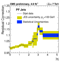
Figure 1: PU Energy vs number of primary vertex and Relative Factor vs $|\eta|$

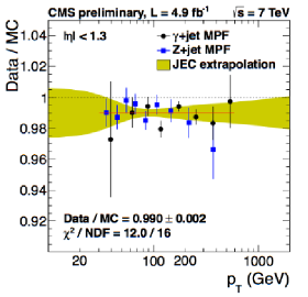
Figure 2: $p_{T}$ dependent correction factor

4 Jet Cross-Section Measurement

In proton-proton collision, the total scattering cross section is computed convoluting the parton distribution function (PDF) of each incoming parton from each proton with the corresponding partonic level cross section. At leading order (LO), the jets are produced via the subprocesses, $qq\to qq$, $q\bar{q}\to q\bar{q}$, $gg\to gg$, $qg\to qg$, $gg\to q\bar{q}$ and $q\bar{q}\to gg$ where the leading partonic level cross section turns out to be $gg\to gg$ because of the large color factors. In Fig. 3, we show the Feynman diagrams for these sub processes. Note that, relative contributions due to these sub channels to the total cross section is a combine effect of initial PDF and the magnitude of partonic level cross section. If the two incoming protons carry four momenta $P_{1}$, $P_{2}$, then the differential total cross section is given by,

$$d\sigma(P_{1},P_{2})=\sum_{a,b}\int\int dx_{1}dx_{2}~{}f_{a}(x_{1},\mu_{F}^{2})~{}f_{b}(x_{2},\mu_{F}^{2})~{}d\hat{\sigma}(p_{1},p_{2},\mu_{R}^{2},\alpha_{S}(\mu_{R}))$$ (2)

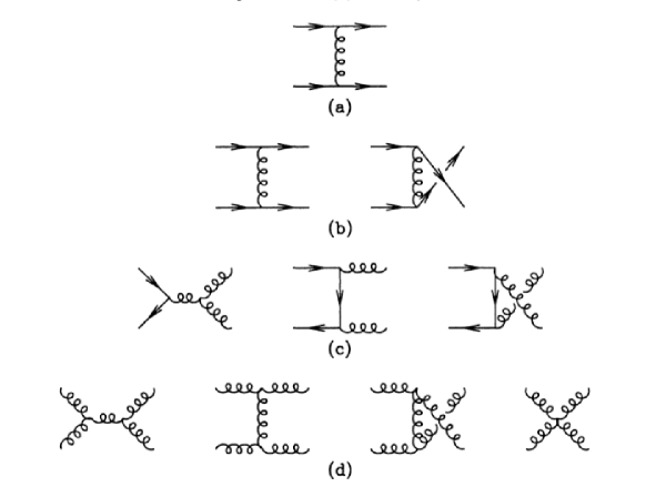
Figure 3: Feynman diagrams for tree level processes contributing in jet production at hadron colliders

Here $p_{1}$, $p_{2}$ are the four momenta of the two incoming partons which take part in the hard interaction and $x_{i}$’s are the Bjorken variables defined to be the momenta fractions $x_{i}~{}=~{}p_{i}/P_{i}$, for $i=1,2$. The sum over indices $a$ and $b$ run over different flavors of incoming partons. The scales $\mu_{F}$, $\mu_{R}$ denote the factorization and renormalization scales respectively, $\alpha_{S}(\mu_{R})$ is the strong coupling constant evaluated at the scale $\mu_{R}$. The $\hat{\sigma}$ is the partonic level cross section calculated using the principles of pQCD. The LO QCD cross section is enormous which is of the order of $\sim\alpha_{s}^{2}$ is found to be $\sim$ $10^{8}$pb for $p_{T}\geq$10 GeV and comes down to $10^{5}$pb for $p_{T}\geq$100 GeV for $\sqrt{s}=$7 TeV. Since it is predominantly a QCD process and mediated by gluon, an uncertainty due to the choice of scales and also PDF is expected to be very large($\sim$100%). Therefore, in order to obtain a reliable estimate of the jet cross section, one needs to consider next to leading order (NLO) terms in perturbation theory. Currently the NLO jet cross section is computed maximum up to 5 jets final state [67]. In this study the NLO calculation for jet cross section is performed using NLOJet++[68] package.

4.1 Jet and Event Selection

As mentioned in the previous section, in the CMS experiment jets are reconstructed using anti-$k_{T}$ [51] algorithm built in FastJet package [54] with the size parameter R=0.7. The choice of larger value for R allows to cluster more hard scattered partons and hence the jet energy and dijet mass resolution is increased compared to smaller value of $R$. A jet with energy $E$ and momentum components $\vec{p}~{}=~{}(p_{x},p_{y},p_{z})$ will have transverse momentum $p_{T}~{}=~{}\sqrt{p_{x}^{2}+p_{y}^{2}}$. In this measurement high quality of events are ensured by imposing certain selection criteria. For example, the event should have a good reconstructed primary vertex to which at least four well reconstructed tracks are associated. The vertex should be within a distance along the z axis (original beam direction) from the center of the detector ($|z|<24$cm) and in the x-y plane (transverse to z axis) it can be shifted at most 2cm ($\sqrt{x^{2}+y^{2}}<2$cm). Indeed any pure QCD event is expected to have a negligible missing transverse energy (MET), as defined, $\vec{{\not\!E}_{T}}~{}=~{}-\sum_{i}(E_{i}~{}\sin\theta_{i}~{}\cos\phi_{i}~{}\hat{x}~{}+~{}E_{i}~{}\sin\theta_{i}~{}\sin\phi_{i}~{}\hat{y})$, the summation over $i$ runs over all the reconstructed particles in the event. $E_{i}$ is the energy of the $i$ th particle, and $\theta_{i}$,$\phi_{i}$ are the polar and azimuthal angle of the corresponding particles measured with respect to $\hat{z}$, the initial beam direction, $\hat{x},\hat{y}$ are the unit vectors along $x$ and $y$ axis respectively. Naturally, the ratio, $|\vec{{\not\!E}_{T}|}/\sum_{i}E_{T}^{i}$ is a good discriminator to isolate pure QCD events as shown in Fig. 4, where it is shown for both data and MC corresponding to inclusive jet(left) and dijet events(right) [66]. We choose to apply an upper cut 0.3 to select genuine QCD events rejecting any contribution due to noise of any miss calibration of the detector. A long tail of $|\vec{{\not\!E}_{T}|}/\sum_{i}E_{T}^{i}$ beyond 0.4 may be due to events from $Z$+jets, where $Z\rightarrow\nu\bar{\nu}$ process leads to a high missing energy.

Figure 4: $|\vec{{\not\!E}_{T}|}/\sum E_{T}$ distribution with inclusive jet and dijet event selection criteria

Once a good event is selected then jets are formed by clustering the stable particles reconstructed by PF technique in the event. Reconstructed jets are checked with the jet identification criteria to ensure good quality of jets originating from hard scattered partons and not due to some detector level noise. The tight jet identification criteria applied in CMS is the following [66]
•At least one PF particle.
•Charged hadron energy fraction and multiplicity $\geq 0$ in the region $|\eta|\leq 2.4$. •Neutral hadron energy fraction $\leq 0.9$.
•Photon energy fraction $\leq 0.99$ .
•Muon energy fraction $\leq 0.9$.
•Electron energy fraction $\leq 0.9$.
In addition, as discussed in previous section, energy correction is required on the measured jet energy to account for the non-uniform and non-linear response of CMS calorimetric system. After the jet energy correction is applied, the measured momenta are corrected to the particle level. The events, produced after proton-proton collision, are filtered by a trigger system and then stored. In CMS, trigger is a two tier system, Level-1 [69] and High Level Trigger (HLT) [70]. The former one is mainly a hardware based trigger whereas the later one is a software based trigger.

The data which is analyzed for this measurement collected by six HLT of $p_{T}$ thresholds 60, 110, 190, 240, 370 GeV. Events consisting at least one jet with corrected jet $p_{T}$ greater than the trigger threshold are stored. The on line triggered jets are calorimeter jets with worse resolution where as off-line jets are constructed by particle flow technique and has better resolution compared to calorimeter jets. The triggers with lower $p_{T}$ thresholds have high prescale factors to fit the trigger bandwidth due to the high QCD event rates and hence have low effective luminosity. In Table 1 we show the individual HLT paths with the corresponding effective integrated luminosities. In order to achieve full trigger efficiency, we apply a off-line cuts on PF jet $p_{T}\geq$ 114, 196, 300, 362 and 507 GeV for each HLT triggers respectively. The inclusive jet cross section measurement is carried out up to a rapidity 2.5 in an equal bins of $\Delta y=0.5$. For the dijet mass measurement, at least two jets with momenta $p_{T1}\geq 60$ GeV and $p_{T2}\geq 30$ GeV are required in the event. The cross section is measured in the bins of maximum rapidity $y_{max}=max(|y_{1}|,|y_{2}|)$. Low $y_{max}$ value probe the large angle of scattering in the s-channel while higher value of $y_{max}$ probe small-angle scattering in t-channel.

HLT $p_{T}$ ($GeV$)	60	110	190	240	370
$L_{eff}~{}(pb^{-1})$	0.4	7.3	152	512	4980

Table 1: HLT Triggers And Effective Luminosities

4.2 $p_{T}$ and $M_{jj}$ Measurement

The pure QCD events, in collected data sample, are isolated requiring jets and events should pass certain selection criteria as described in the previous section. The distribution of transverse momentum of jets, $p_{T}$ are obtained dividing the entire $p_{T}$ range into 21 bins for six rapidity intervals with $\Delta|y|$=0.5 and also similarly for dijet invariant mass ($M_{jj}$) spectra are obtained. The entire range of $p_{T}$ distribution is obtained corresponding to each five different HLT paths. The reconstruction of each segment of the spectrum is obtained only by one trigger path avoiding double counting of jets. Eventually, the measured yields are transformed to double-differential inclusive-jet cross sections as:

$$\frac{\text{d}^{2}\sigma}{\text{d}p_{T}\text{d}|y|}=\frac{1}{\epsilon\mathcal{L}}\frac{N}{\Delta p_{T}\Delta|y|}\text{,}$$ (3)

where $N$ is the number of jets in the corresponding $p_{T}$ bin, $\mathcal{L}$ is the effective integrated luminosity of the data sample taking into account the trigger prescales. Here $\epsilon$ is the product of the trigger and jet selection efficiencies, $\Delta p_{T}$ and $\Delta|y|$ are the corresponding bin widths. Notice that the bin-width increases progressively, proportional to $p_{T}$ resolution. By a similar fashion, the double differential cross section for di-jet mass distribution is obtained as,

$$\frac{d^{2}\sigma}{dM_{jj}d|y|}=\frac{1}{\epsilon\mathcal{L}}\frac{N}{\Delta M_{jj}\Delta|y|}\text{,}$$ (4)

where the symbols represent identical meaning as the previous equation, eq.3, $\Delta M_{jj}$ is the dijet invariant mass bin width which increases progressively as well, equal or larger than $\Delta M_{jj}$ resolution.
Fig. 5 shows the measured differential cross-section for various $p_{T}$ (left) and $M_{jj}$ (right) as directly measured from data for the central rapidity bin. Each region of $p_{T}$ or $M_{jj}$ is constructed using the particular HLT. Notice that, for $\sqrt{s}~{}=~{}7$ TeV, $p_{T}$ extends up to $\sim$ 2 TeV and $M_{jj}$ extends up to $\sim$ 4 TeV.

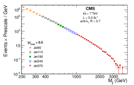
Figure 5: Measured jet yield scaled by the trigger prescale factor for inclusive jet production on left pannel and on right panel the same distributions shown for dijet mass distribution for the central rapidity bin $|y|<0.5$.

The statistical uncertainty in the number of jets in a bin is
$e_{stat}~{}=~{}\sqrt{(4-3f)/(2-f)}.\sqrt{N_{jets}}$, where $f~{}=~{}N_{1}/N_{ev}$ is the fraction of events that contribute one jet in the given bin. The formula is valid under the assumption that the number of events that contribute more than two jets in each bin is negligible, which has been verified for the current measurement.

In Fig. 6, we present the inclusive jet $p_{T}$ spectrum on the left and the di-jet mass spectrum on the right for various $y$ bins corresponding to ${\cal L}=5fb^{-1}$. The distributions are scaled up by a factor for better presentation as shown in the plot. The theory predictions are estimated, as mentioned before, by using NLOJet++ [68] and NNPDF2.1 PDF [71] sets and the comparison is shown in both the figures. The QCD scales, both $\mu_{R}$ and $\mu_{F}$ are set to jet $p_{T}$ for inclusive jet spectrum and average $p_{T}$ of two jets in case of di-jet spectrum. The NLO spectrum also corrected for non-perturbative effects which will be discussed in Section 7.

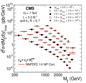
Figure 6: $\rm NLO\times\rm NP$ theory prediction (with NNPDF2.1 PDF set) is compared with the measured spectrum up to rapidity $|y|=2.5$ at an interval of 0.5

5 Unfolding

In any experimental measurement one of the goal is to compare between data and theory predictions or with results from other experiments. However in this measurement, finite detector resolution smear the physical quantities and as a consequence the measured observables are expected to differ from the corresponding true values. Therefore in order to carry out a realistic comparison, it is required to make measured observable free from any detector effects, namely unfold the data to be compared with known theory prediction. Unfolding is a procedure used to get rid of all detector level distortion from the measured spectrum.

It is a standard practice, for the measurement of a single observable, to apply $bin-by-bin$ correction in the measured observable. In this method one evaluates the generalized efficiency, which is defined as the ratio of number of events falling in a certain bin of the observed spectrum to the number of events in the same bin in the true spectrum. The large number of simulated events are used to obtain this ratio for each bin of the observable. In general this efficiency can be larger than unity depending upon the number of events migrating away or towards a particular bin due to detector smearing. The major short falling of this method is that it fails to take care large bin migration of events and also it doesn’t take into account the unavoidable bin to bin correlations between adjacent bins. A method which overcomes this shortcomings is the regularized unfolding technique [72]. One of the most popular unfolding technique of this class is Bayesian unfolding [73]. The main essence of this algorithm lies with the treatment of different bins of the true distribution as independent, i.e. without any correlation among each other and as a result it works for any kind of smearing. The core part of the algorithm is that it knows only about ’cause cells’ (number of events in a bin for true distribution) and ’effect cells’ (number of events in a bin for smeared distribution), but it doesn’t know the position of the cells in the configuration space. The final goal of the problem is to estimate the probability of finding the true number of events in a given bin when the measured spectrum and some apriori knowledge on the detector smearing is available.

In the Bayesian unfolding process ([73, 74]), the number of estimated events in the $i$-th bin of the unfolded distribution (’estimated causes’) $\hat{n}(C_{i})$, as the result of applying the unfolding matrix $M_{ij}$ on the $j$-th bin of raw distribution (’effects’), containing $n(E_{j})$ events, is given by:

$$\hat{n}(C_{i})=\sum_{j=1}^{n_{E}}M_{ij}n(E_{j}),$$ (5)

where

$$M_{ij}=\frac{P(E_{j}|C_{i})n_{0}(C_{i})}{\epsilon_{i}\sum_{l=1}^{n_{C}}.P(E_{j}|C_{l})n_{0}(C_{l})}$$ (6)

Here $P(E_{j}|C_{i})$ is the $n_{E}\times n_{C}$ response matrix, where $n_{E}$ and $n_{C}$ are the number of bins in measured and unfolded distributions respectively. This response matrix causes correlation among different bins in the unfolded distribution. Fig 7 shows an example of response matrix for inclusive and dijet measurement used in the 7 TeV measurement.

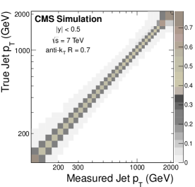
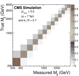
Figure 7: Response matrix for the central rapidity bin for inclusive and dijet measurement.

Here $\epsilon_{i}$ = $\sum_{j=1}^{n_{E}}P(E_{j}|C_{i})$ are efficiencies for each bin and $n_{0}(C_{l})$ is the number of entries in the $l$-th bin of the prior distribution. Output of each iteration of unfolding, goes as prior distribution to the next iteration.

Covariance matrix for unfolding is calculated by error propagation from $n(E_{j})$ which is denoted as $V(\hat{n}(C_{l}),\hat{n}(C_{m}))$. $M_{ij}$ is independent of $n(E_{j})$ for the first iteration only. So the error propagation from one iteration to another is described in form of a matrix which is given by [74],

$$\frac{\partial\hat{n}(C_{i})}{\partial n(E_{j})}=M_{ij}+\sum_{k=1}^{n_{E}}M_{ik}~{}n(E_{k})\bigg{(}\frac{1}{n_{0}(C_{i})}\frac{\partial n_{0}(C_{i})}{\partial n(E_{j})}~{}-~{}\sum_{l=1}^{n_{C}}\frac{\epsilon_{l}}{n_{0}(C_{l})}\frac{\partial n_{0}(C_{l})}{\partial n(E_{j})}M_{lk}\bigg{)}.$$ (7)

This depends upon the matrix elements $\frac{\partial n_{0}(C_{i})}{\partial n(E_{j})}$, which is $\frac{\partial\hat{n}(C_{i})}{\partial n(E_{j})}$ from the previous iteration. For the first iteration, the L.H.S of the eq. 6 is purely $M_{ij}$. The covariance matrix of the unfolded distribution is obtained from the error propagation matrix as [74],

$$V(\hat{n}(C_{k}),\hat{n}(C_{l}))=\sum_{i,j=1}^{n_{E}}\frac{\partial\hat{n}(C_{k})}{\partial n(E_{i})}~{}V(n(E_{i}),n(E_{j}))\frac{\partial\hat{n}(C_{l})}{\partial n(E_{j})}.$$ (8)

from the covariance matrix of the measurement $V(n(E_{i}),n(E_{j}))$.

In the present study the goal is to compare $p_{T}$ and $M_{jj}$ spectrum with the theory prediction which requires to unfold the corresponding spectrum. Here in each $p_{T}$ or $M_{jj}$ bin is populated by jet yield that migrate from the neighboring bins. A fraction of yield from a particular bin also migrate to the neighboring bins due to resolution effects. In a steeply falling spectrum, like in the case of QCD, the net effect is that for all the bins, number of jets migrate in is much more than the number of events that migrate out. In the process of unfolding, the first task is to construct a response matrix $\mathcal{R}$ of size $M\times N$, where $N$ is the number of bins in the measured spectrum, and the $p,q$ th element of this matrix gives the correlation between the $p$-th and $q$-th bin of measured and true spectrum respectively. This response matrix $\mathcal{R}$ is operated on the measured spectrum to get the unfolded spectrum. The response matrix is created from simulation and the difference between data and simulation in terms of jet energy resolution has been accounted. The unfolding is done by DiAgostini’s iterative Bayesian unfolding method with iteration parameter equal to 4. Of course, the unfolded spectrum does not describe precisely the true spectrum, it represent it with certain uncertainty, which will be discussed later.

6 Experimental Uncertainty

The experimental uncertainty refers to all the uncertainties related with the measurements that affect the $p_{T}$ and $M_{jj}$ spectrum. The leading components of the uncertainties are due to jet energy scale (JES), jet energy resolution (JER) and the luminosity uncertainty. The other uncertainty sources like angular resolution has very less effect on the measured spectrum. For the inclusive-jet measurement, the total relative uncertainty from all the sources varies between $10\%$ to $35\%$ as we move from lower $p_{T}$ to higher while for the dijet mass measurement it varies between $5\%$ to $35\%$ for the entire mass range. On the other hand for both the measurements, the amount of relative uncertainty increases with the rapidity bins. The description of various uncertainty sources are given in the following sub-section.

6.1 Jet Energy Scale Uncertainty

The jet energy scale(JES) is the most dominant component of total uncertainty in the measurement involving $p_{T}$ of jets. Since we are dealing with a very steeply falling spectrum in QCD($\sim~{}1/p_{T}^{4}$), so a small uncertainty($\delta p_{T}$) in the measurement translates significant uncertainty in the measurement of cross-section. The JES uncertainty on the PFJets is of order of 2% to 2.5% for the 7 TeV measurement. The JES sources contain eleven mutually uncorrelated components, each representing a signed $1\sigma$ fluctuation from the central value for each $p_{T}$ and $\eta$ bin and it is parametrized within the physically allowed $p_{T}$ and $\eta$ ranges [66]. Summing up the each contribution in quadrature gives the total JES uncertainty. The uncertainty sources are broadly divided into three categories. They are viz. PU effects, relative calibration of jet energy scale vs $\eta$ and absolute energy scale including $p_{T}$ dependence.

Although the JES uncertainty for the PU effects are mainly significant at very low $p_{T}$, but for 7 TeV measurement it is not so much significant. The second broad category of uncertainty is due to L2 correction, mentioned in section 3.2. It parametrizes the possible variation of the JES, and it is directly measured as the correlation between different $\eta$ values for a fixed $p_{T}$ bin. In general the uncertainties can be $p_{T}$ dependent. However a detail study of data and MC showed that this dependence can be factorized without any loss of generality.

The last category is the absolute scale uncertainty or the uncertainty introduced due to L3 correction, the most relevant one for the jet cross-section measurement analysis. The well measured $p_{T}$ balanced events are used to calibrate this $p_{T}$ dependent uncertainty, as mentioned in section 3.2. This calibration is used to constrain the JES in a finite $p_{T}$ region of $30-600~{}GeV$. The JES beyond this regions are obtained from MC simulation. The $p_{T}$ dependent uncertainty arising from modeling of underlying event and jet fragmentation is obtained by comparing predictions from PYTHIA6 [64] and HERWIG++ [75]. The general studies show that both the generators in general agree well with data. The uncertainty due to calorimetric response to hadrons is estimated varying the response parametrization by $\pm 3\%$ and comparing with the central value. The luminosity uncertainty for 7 TeV measurement is about $2.2\%$ which is $100\%$ correlated among different $p_{T}$ bins.

Fig 8 shows the uncertainties in the cross section measurement due to different components of total systematics for a wide range of $p_{T}$ and $M_{jj}$. As mentioned before, the most dominant contribution to the total uncertainty in the cross section is due to JES. In the measurement of inclusive jet cross section, the total uncertainty is about 5-20% (10-30%), where as for dijet mass measurement it varies between 5-30% (10-60%) for central (outermost) rapidity bin in both the cases.

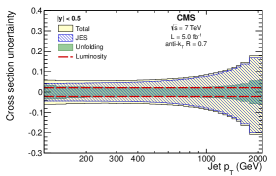
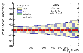
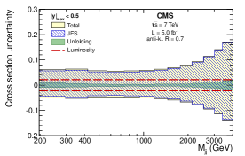
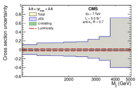
Figure 8: Relative experimental uncertainties for inclusive jet and Dijet mass measurement.

6.2 Unfolding Uncertainty

The unfolding correction is directly related to $p_{T}$ and $M_{jj}$ resolution. In case of dijet mass the resolution varies between $2\%$ to $5\%$ in all rapidity bins and becomes larger as the dijet mass increases. For inclusive jet, the same varies between $5\%$ to $10\%$ and the uncertainty increases with increasing jet $p_{T}$.

7 Theory Calculation

Once the experimental measurement is performed, the next task is to compare the theory predictions with the unfolded measured spectrum. It is reasonable and relatively precise to use NLO calculation to predict theoretical values of cross section. Furthermore, NP correction factor is applied to account for effect due to hadronization and multiparton interaction (MPI). These are discussed briefly in the next section.

7.1 NLO Calculations

In hadron collision, the QCD jet cross sections are available for a long time  [76, 77, 78, 79]. The recent NLO calculation for three jet observables are also performed [68]. Here the NLO jet cross-sections are estimated using NLOJet++ which is based on the calculation described in Ref. [68]. However, since the NLO calculation is very much time consuming, it is optimized within the framework of fastNLO(v1.4) [80] package. In calculating jet cross sections one needs to provide PDF and QCD scales which are not exactly defined. As a consequence, theory calculations are subject to some uncertainties due to the various choices of PDFs and QCD scales. The renormalization ($\mu_{R}$) and factorization ($\mu_{F}$) scales for the inclusive and dijet measurements, are set equal to the jet $p_{T}$ and the average transverse momentum of the two jets($p_{T}^{Avg}=\frac{p_{T}^{1}+p_{T}^{2}}{2}$), respectively. The NLO calculation is done with five different PDF sets: CT10 [81], MSTW2008NLO [82], NNPDF2.1 [71], HERAPDF1.5 [83], and ABKM09 [84] at the corresponding default values of the strong coupling constant $\alpha_{S}(M_{z})$= 0.1180, 0.120, 0.119, 0.1176, and 0.1179, respectively.

7.2 Non Perturbative Correction

As explained before in p-p collision, due to hard interaction colored partons(quarks and gluons) are produced and subsequently they undergo cascades and produce various colored combination of quarks and anti-quarks which finally recombine among themselves to produce colorless hadrons which hit the detector. This is a process called fragmentation or hadronization. These colorless hadrons, primarily K and $\pi$ mesons enter into detector and deposit energy in its different components. In contrast to hard interaction which is a short distance effect, this process is a long distance effects and occurs at very low energy scale where the strong couplings constant $\alpha_{s}$ becomes too large and perturbation theory fails. Hence, the hadronization is pure non-perturbative effects which cannot be estimated using techniques of pQCD. Moreover, in p-p collision the hard partons from protons which share a fraction of initial beam energy produce hard scattered events leaving the rest of the partons as beam remnant of protons. Therefore, any hard interaction is also accompanied by many soft interactions among this remnant of protons, which is known as multiple parton interaction (MPI). Note that MPI also cannot be described from the first principles of QCD, it is also a purely NP effect. Therefore, parton level cross sections are required to be corrected to obtain particle level cross section. This non perturbative(NP) correction factor accounts for the amount of correction required due to hadronization and MPI bin-by-bin. This correction is estimated by taking the ratio of the cross section predicted with the nominal settings for MPI and hadronization model parameters and the cross section obtained without any effects of MPI and hadronization. The NP correction factor is defined as $c_{NP}~{}=~{}\frac{\sigma(Nominal)}{\sigma(NoMPI,NoHAD)}$. The numerator is the cross-section with the nominal settings for MPI and hadronization in the generators, where as the denominator represents the same without any of these effects.
These are estimated from MC simulation using two different generators
PYTHIA6(tune Z2) [64] and HERWIG++ [75]. The chosen MC models are representative of the possible values of the non-perturbative corrections, due to their different physics description. The average value of the NP correction factor is estimated as the mean value from two different generator for each $p_{T}$ and $M_{jj}$ bin. The uncertainty due to NP correction is estimated as the difference between the values obtained from two different generators, for each bin. Eventually to obtain the full theory spectrum correctly, NP correction factor is multiplied with the NLO theory prediction. In this measurement, the NP correction varies from 1% to 20%  [66].

7.3 Theoretical Uncertainty

The variation among different sets of PDF introduces a total uncertainty up to $30\%$ on the theoretical prediction of the cross-section for both inclusive-jet and dijet measurements. On the other hand, the variation of $\alpha_{S}(M_{z})$ by 0.001 translates $1-2\%$ uncertainty on total cross-section. The scale uncertainty is determined by varying the renormalization and factorization scale for six different points ($\mu_{F}/\mu,\mu_{R}/\mu)=(0.5,0.5)$, $(2,2)$, $(1,0.5)$, $(1,2)$, $(0.5,1)$, $(2,1)$, where $\mu=Jet~{}p_{T}$ for inclusive jets and $\mu=p_{T}^{Avg}$ for dijet measurement.

In Fig. 9 and Fig. 10, we demonstrate the total uncertainty on the theory cross section calculation due to different sources namely PDF, QCD scale and NP for a wide range of $p_{T}$ and for two extreme bins of rapidity, taking NNPDF2.1 as the benchmark PDF. Note that for the barrel region, the uncertainty is within 5% for the range of $p_{T}$ upto $\sim$ 1 TeV and thereafter it increases. In case of outer most rapidity bin, uncertainty becomes large(more than 10% or above) for $p_{T}$ beyond 500 GeV. Notice that, uncertainty due to PDF dominates over the others. Similarly, in Fig. 10 the uncertainties on dijet cross section predictions are shown for various $M_{jj}$ values for two rapidity bins. In this case the uncertainty due to NP corrections large at lower bins of $M_{jj}$. Evidently, PDF uncertainty contributes most to the total theoretical uncertainty.

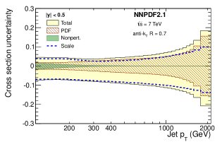
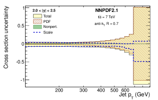
Figure 9: Different components of total theoretical uncertainty for inclusive jet, for two different rapidity bins.

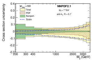
Figure 10: Different components of total theoretical uncertainty for dijet jet, for two different rapidity bins.

8 Results

The inclusive jet cross section in terms of double differential measurement are compared with data for five different PDF sets as mentioned before and for five rapidity bins [66].

Figure 11: Data over theory for NNPDF2.1 theory prediction of inclusive jet $p_{T}$. for two extreme rapidity bins.

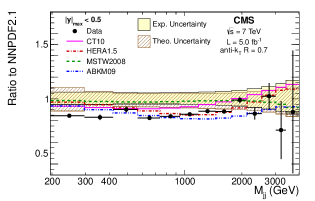
Figure 12: Data over theory for NNPDF2.1 theory prediction of dijet mass for two extreme rapidity bins.

For the sake of illustration, in Fig. 11 and  12 the theory prediction based on NNPDF2.1 is compared with data for both inclusive and dijet cases and are shown for two extreme rapidity bins, viz. $0.0<|y|<0.5$ and $2.0<|y|<2.5$, along with total experimental and theoretical uncertainties. Note that the total experimental uncertainty is comparable with the theoretical uncertainty. Clearly, in both cases, this ratio is within the band of uncertainty($\sim 8-10$%). The error bars are too large for high $p_{T}$ or $M_{jj}$ range, and is dominantly due to statistical uncertainty. Similar pattern of agreement is observed for other PDF sets as well, except for ABKM09 set, in which case this ratio goes out of the error band for the low rapidity bins, $|y|<$1 [37]. However, a good agreement between theory and data is observed as presented in Fig. 11,12.

The detail studies are also carried out to understand data and theory compatibility by comparing their ratio using the central value of each PDF sets. In Fig. 11 and Fig. 12, we demonstrate this comparison for NNPDF2.1 PDF set for inclusive and dijet mass measurement respectively. In the same Figures the other curves represent the ratio between the calculations based on NNPDF2.1 and other PDF sets, like ABKM09, CT10, HERAPDF1.5, MSTW2008NLO as shown. Here the results are presented for two rapidity bins, however, the studies are done for all rapidity bins [37]. In case of inclusive jet data, for central region, the agreement for NNPDF2.1 PDF set is within 5-10% for a wide range of $p_{T}$, but for higher $p_{T}$($>$1 TeV), it is affected by large uncertainty. This conclusion remains true also for 2.0$<|y|<$2.5 bin, where the total uncertainty is too large, in particular for high $p_{T}$ range. Similar level of agreement is also observed for di-jet case and but, at larger values of $M_{jj}$, the uncertainty is too large, so it is far from any conclusion to be drawn. In both cases more or less similar type of behavior of ratio measurements are observed.

9 Summary

The inclusive jet cross section and dijet invariant mass measurement are reviewed here with some detail discussions. In this measurement the important quantities to be measured are the momentum and energy of jets which is a very non trivial objects from both theoretical and experimental perspective. Before describing this measurement we discuss various issues related with jets. In the formation of jets, the main constituents are either four momenta of reconstructed stable particles or four momenta of calorimeter towers which are combined to obtain the kinematic properties of jets. The combination methods of momentum of jet constituents are guided by certain theoretical prescriptions, which take into account singularities, present due to the very soft or collinear branching of the partons. In order to avoid these theoretical problems, the jet algorithms are properly designed, resulting the evolution of various types of jet algorithms. In this context the anti-$k_{T}$ jet algorithm is also discussed, which is currently the most widely used algorithm in hadron collider experiments.

The different techniques adopted in CMS for jet reconstruction and JES are discussed. Due to the non linear response of the detector, the measured jet energy requires to be corrected. The various sources of this correction factors are presented and it is found that the derived JEC from $\sqrt{s}=7$ TeV and $\int L$ = 5${\rm fb}^{-1}$ data is at-most 20%. In performing this measurement the details of the selection of good quality of events and jets are presented including a short description of implemented trigger system in CMS. Finally the results of this measurement are presented in terms of double differential cross section for a wide range of $p_{T}$ and $\rm{M}_{jj}$ for a five regions of rapidity bins covering $0\leq{\rm|y|}\leq 2.5$ with an interval $\Delta|y|~{}=$ 0.5.

Realistically, to make a comparison of this measurements with theory prediction or results obtained by other experiments, it is required to eliminate smearing effects of the detector in the measurement, which is a delicate task. Thus, the unfolding of data, the corresponding algorithm and how it is implemented in this particular measurement are described in details. Moreover, measurements are also affected by different type of systematics including statistical uncertainties, which all are need to be accounted. It has been observed that the main source of uncertainty is primarily due to JES, which varies between 2-2.5% and translates an uncertainty 5-35% on the measured inclusive jet cross section across varying $|y|$ and $p_{T}$ bin. The same JES uncertainty for the dijet mass cross section shoots up to 60% for the outermost rapidity bin.

On the other hand, the theory prediction based on LO calculation is not adequate to describe this process. Hence the theoretical estimations are obtained based on NLO calculation and is performed for five different PDF sets viz. ABKM09, HERA15, CT10, MSTW2008 and NNPDF2.1. Of course, the various sources of uncertainties in these predictions are mentioned and it is observed that choice of various PDF is the dominant source of theoretical uncertainty which is about 30% on calculated cross section. In addition, a non-perturbative correction, arising due to the multiple parton interaction and hadronization effects, is applied to these NLO theory prediction. Eventually, the comparison between data and theory predictions are presented along with the total theoretical and experimental uncertainty limits. It is found both the measurements, inclusive jet and dijet mass cross sections, and theory predictions agree within 10% and this deviation is in general covered by the total theoretical and experimental uncertainty limits.

This measurement confirms once more the success of pQCD with a very high precision unambiguously at the probed energy regime. This measurement probes a wide region in phase-space. The inclusive jet $p_{T}$ varies between 100 GeV to 2 TeV, whereas the dijet invariant mass extends up to 5 TeV. The momentum fraction carried by the partons, $x$, probed in this experiment $0.03<x<0.57$. The application of this measurements are very wide, for instance, it can be used for extraction of the strong coupling constant $\alpha_{S}$ and testing its evolution with energies as predicted by the theory QCD. Furthermore, this measurement can be used to constrain the parameters of different PDF sets as well.

Acknowledgements
The authors acknowledge the CMS collaboration and the India-CMS collaboration for their support. They are also grateful to Bora Isildak, Mithat Kaya, Ozlem Kaya, Konstantinos Kousouris, Klaus Rabbertz, Mikko Voutialinen, Niki Saoulidou, Maxime Gouzevitch, Sung-Won Lee and Jeffrey Berryhill for discussion on several occasion.

References

- [1] J. Collins, Foundations of Perturbative QCD. Cambridge University Press, 2011. http://dx.doi.org/10.1017/CBO9780511975592.
- [2] W. J. S. R. K. Ellis and B. R. Webber, QCD and Collider Physics. Cambridge University Press, 1996. http://dx.doi.org/10.1017/CBO9780511628788.
- [3] I. K. G. Dissertori and M. Schmelling, Quantum Chromodynamics: High energy experiments and theory. Oxford University Press, 2009. http://ukcatalogue.oup.com/product/9780199566419.do#.UaSfkhVQoVI.
- [4] G. Altarelli, “Experimental tests of perturbative qcd,” Annual Review of Nuclear and Particle Science 39 no. 1, (1989) 357–406, http://www.annualreviews.org/doi/pdf/10.1146/annurev.ns.39.120189.002041. http://www.annualreviews.org/doi/abs/10.1146/annurev.ns.39.120189.00204%1.
- [5] A. Banfi, “Event shapes at hadron colliders,” PoS DIS2010 (2010) 099, arXiv:1101.0148 [hep-ph].
- [6] ATLAS Collaboration, G. Aad et al., “Measurement of event shapes at large momentum transfer with the ATLAS detector in collisions at TeV,” Eur.Phys.J. C72 (2012) 2211, arXiv:1206.2135 [hep-ex].
- [7] CMS Collaboration, V. Khachatryan et al., “First Measurement of Hadronic Event Shapes in Collisions at TeV,” Phys.Lett. B699 (2011) 48–67, arXiv:1102.0068 [hep-ex].
- [8] S. D. Ellis, C. K. Vermilion, J. R. Walsh, A. Hornig, and C. Lee, “Jet Shapes and Jet Algorithms in SCET,” JHEP 1011 (2010) 101, arXiv:1001.0014 [hep-ph].
- [9] CMS Collaboration, S. Chatrchyan et al., “Shape, transverse size, and charged hadron multiplicity of jets in pp collisions at 7 TeV,” JHEP 1206 (2012) 160, arXiv:1204.3170 [hep-ex].
- [10] ATLAS Collaboration, G. Aad et al., “Study of jet shapes in inclusive jet production in collisions at using the atlas detector,” Phys. Rev. D 83 (Mar, 2011) 052003. http://link.aps.org/doi/10.1103/PhysRevD.83.052003.
- [11] CDF Collaboration, T. Affolder et al., “Measurement of the strong coupling constant from inclusive jet production at the tevatron collider,” Phys. Rev. Lett. 88 (Jan, 2002) 042001. http://link.aps.org/doi/10.1103/PhysRevLett.88.042001.
- [12] CMS Collaboration, S. Chatrchyan et al., “Measurement of the ratio of the inclusive 3-jet cross section to the inclusive 2-jet cross section in pp collisions at = 7 TeV and first determination of the strong coupling constant in the TeV range,” arXiv:1304.7498 [hep-ex].
- [13] B. Malaescu and P. Starovoitov, “Evaluation of the strong coupling constant using the atlas inclusive jet cross-section data,” The European Physical Journal C 72 no. 6, (2012) 1–14. http://dx.doi.org/10.1140/epjc/s10052-012-2041-y.
- [14] D0 Collaboration, S. Abachi et al., “Direct measurement of the top quark mass,” Phys. Rev. Lett. 79 (Aug, 1997) 1197–1202. http://link.aps.org/doi/10.1103/PhysRevLett.79.1197.
- [15] CMS Collaboration, S. Chatrchyan et al., “Measurement of the top-quark mass in t-tbar events with lepton+jets final states in pp collisions at sqrts=7 tev,” Journal of High Energy Physics 2012 no. 12, (2012) 1–37. http://dx.doi.org/10.1007/JHEP12%282012%29105.
- [16] ATLAS Collaboration, G. Aad et al., “Measurement of the top quark mass with the template method in the t-tbar lepton+jets channel using atlas data,” The European Physical Journal C 72 no. 6, (2012) 1–30. http://dx.doi.org/10.1140/epjc/s10052-012-2046-6.
- [17] ATLAS Collaboration, G. Aad et al., “Search for resonances decaying into top-quark pairs using fully hadronic decays in pp collisions with atlas at =7 tev,” Journal of High Energy Physics 2013 no. 1, (2013) 1–50. http://dx.doi.org/10.1007/JHEP01%282013%29116.
- [18] G. Aad et al., “A search for t-tbar resonances in lepton+jets events with highly boosted top quarks collected in pp collisions at = 7 tev with the atlas detector,” Journal of High Energy Physics 2012 no. 9, (2012) 1–45. http://dx.doi.org/10.1007/JHEP09%282012%29041.
- [19] CMS Collaboration, S. Chatrchyan et al., “Search for z’ resonances decaying to t-tbar in dilepton+jets final states in pp collisions at tev,” Phys. Rev. D 87 (Apr, 2013) 072002. http://link.aps.org/doi/10.1103/PhysRevD.87.072002.
- [20] R. M. Harris and K. Kousouris, “Searches for Dijet Resonances at Hadron Colliders,” Int.J.Mod.Phys. A26 (2011) 5005–5055, arXiv:1110.5302 [hep-ex].
- [21] CMS Collaboration, S. Chatrchyan et al., “Search for supersymmetry in hadronic final states with missing transverse energy using the variables and b-quark multiplicity in pp collisions at = 8 TeV,” arXiv:1303.2985 [hep-ex].
- [22] G. Aad et al., “Search for pair production of massive particles decaying into three quarks with the atlas detector in =7 pp collisions at the lhc,” Journal of High Energy Physics 2012 no. 12, (2012) 1–42. http://dx.doi.org/10.1007/JHEP12%282012%29086.
- [23] J. M. Butterworth, A. R. Davison, M. Rubin, and G. P. Salam, “Jet substructure as a new higgs-search channel at the large hadron collider,” Phys. Rev. Lett. 100 (Jun, 2008) 242001. http://link.aps.org/doi/10.1103/PhysRevLett.100.242001.
- [24] G. Aad et al., “Jet mass and substructure of inclusive jets in = 7 tev pp collisions with the atlas experiment,” Journal of High Energy Physics 2012 no. 5, (2012) 1–47. http://dx.doi.org/10.1007/JHEP05%282012%29128.
- [25] F. V. Tkachov, “A Theory of jet definition,” Int.J.Mod.Phys. A17 (2002) 2783–2884, arXiv:hep-ph/9901444 [hep-ph].
- [26] G. F. Sterman, “QCD and jets,” arXiv:hep-ph/0412013 [hep-ph].
- [27] G. P. Salam, “Recent progress in defining and understanding jets,” Acta Phys.Polon.Supp. 1 (2008) 455–461, arXiv:0801.0070 [hep-ph].
- [28] D0 Collaboration, V. Abazov et al., “Measurement of the inclusive jet cross-section in collisions at =1.96-TeV,” Phys.Rev.Lett. 101 (2008) 062001, arXiv:0802.2400 [hep-ex].
- [29] D0 Collaboration, V. Abazov et al., “Measurement of the dijet invariant mass cross section in collisions at TeV,” Phys.Lett. B693 (2010) 531–538, arXiv:1002.4594 [hep-ex].
- [30] CDF Collaboration, A. Abulencia et al., “Measurement of the Inclusive Jet Cross Section using the algorithmin Collisions at = 1.96 TeV with the CDF II Detector,” Phys.Rev. D75 (2007) 092006, arXiv:hep-ex/0701051 [hep-ex].
- [31] UA2 Collaboration, J. Alitti et al., “Inclusive jet cross-section and a search for quark compositeness at the CERN collider,” Phys.Lett. B257 (1991) 232–240.
- [32] ZEUS Collaboration, S. Chekanov et al., “Inclusive jet cross-sections in the Breit frame in neutral current deep inelastic scattering at HERA and determination of alpha(s),” Phys.Lett. B547 (2002) 164–180, arXiv:hep-ex/0208037 [hep-ex].
- [33] ZEUS Collaboration, H. Abramowicz et al., “Inclusive-jet cross sections in NC DIS at HERA and a comparison of the kT, anti-kT and SIScone jet algorithms,” Phys.Lett. B691 (2010) 127–137, arXiv:1003.2923 [hep-ex].
- [34] ATLAS Collaboration, G. Aad et al., “Measurement of inclusive jet and dijet cross sections in proton-proton collisions at 7 TeV centre-of-mass energy with the ATLAS detector,” Eur.Phys.J. C71 (2011) 1512, arXiv:1009.5908 [hep-ex].
- [35] CMS Collaboration, S. Chatrchyan et al., “Measurement of the Inclusive Jet Cross Section in Collisions at TeV,” Phys.Rev.Lett. 107 (2011) 132001, arXiv:1106.0208 [hep-ex].
- [36] CMS Collaboration, S. Chatrchyan et al., “Measurement of the differential dijet production cross section in proton-proton collisions at TeV,” Phys.Lett. B700 (2011) 187–206, arXiv:1104.1693 [hep-ex].
- [37] CMS Collaboration, S. Chatrchyan et al., “Jet cross sections and pdf constraints,” Tech. Rep. CMS-PAS-QCD-11-004, CERN, Geneva, 2011.
- [38] D. Gross and F. Wilczek, “Asymptotically Free Gauge Theories. 1,” Phys.Rev. D8 (1973) 3633–3652.
- [39] H. D. Politzer, “Asymptotic Freedom: An Approach to Strong Interactions,” Phys.Rept. 14 (1974) 129–180.
- [40] G. Hanson, G. Abrams, A. Boyarski, M. Breidenbach, F. Bulos, et al., “Evidence for Jet Structure in Hadron Production by e+ e- Annihilation,” Phys.Rev.Lett. 35 (1975) 1609–1612.
- [41] J. R. Ellis, M. K. Gaillard, and G. G. Ross, “Search for Gluons in e+ e- Annihilation,” Nucl.Phys. B111 (1976) 253.
- [42] G. Sterman and S. Weinberg, “Jets from quantum chromodynamics,” Phys. Rev. Lett. 39 (Dec, 1977) 1436–1439. http://link.aps.org/doi/10.1103/PhysRevLett.39.1436.
- [43] A. De Rujula, J. R. Ellis, E. Floratos, and M. Gaillard, “QCD Predictions for Hadronic Final States in e+ e- Annihilation,” Nucl.Phys. B138 (1978) 387.
- [44] J. E. Huth, N. Wainer, K. Meier, N. J. Hadley, F. Aversa, M. Greco, P. Chiappetta, J. P. Guillet, S. Ellis, Z. Kunszt, and D. E. Soper, “Toward a standardization of jet definitions,”.
- [45] G. Salam, “Towards jetography,” The European Physical Journal C 67 (2010) 637–686. http://dx.doi.org/10.1140/epjc/s10052-010-1314-6.
- [46] UA1 Collaboration, G. Arnison et al., “Hadronic Jet Production at the CERN Proton - anti-Proton Collider,” Phys.Lett. B132 (1983) 214.
- [47] CDF Collaboration, T. Aaltonen et al., “Measurement of the inclusive jet cross section at the fermilab tevatron collider using a cone-based jet algorithm,” Phys. Rev. D 78 (Sep, 2008) 052006. http://link.aps.org/doi/10.1103/PhysRevD.78.052006.
- [48] G. P. Salam and G. Soyez, “A practical seedless infrared-safe cone jet algorithm,” Journal of High Energy Physics 2007 (2007) 086. http://stacks.iop.org/1126-6708/2007/i=05/a=086.
- [49] W. Bartel et al., “Experimental evidence for differences in between quark jets and gluon jets,” Physics Letters B 123 (1983) 460 – 466. http://www.sciencedirect.com/science/article/pii/0370269383909942.
- [50] S. Catani, Y. L. Dokshitzer, and B. Webber, “The perpendicular clustering algorithm for jets in deep inelastic scattering and hadron collisions,” Phys.Lett. B285 (1992) 291–299.
- [51] M. Cacciari, G. P. Salam, and G. Soyez, “The anti- jet clustering algorithm,” Journal of High Energy Physics 2008 (2008) 063. http://stacks.iop.org/1126-6708/2008/i=04/a=063.
- [52] Y. Dokshitzer, G. Leder, S. Moretti, and B. Webber, “Better jet clustering algorithms,” Journal of High Energy Physics 1997 (1997) 001. http://stacks.iop.org/1126-6708/1997/i=08/a=001.
- [53] S. Catani, Y. Dokshitzer, M. Seymour, and B. Webber, “Longitudinally-invariant k-clustering algorithms for hadron-hadron collisions,” Nuclear Physics B 406 (1993) 187 – 224. http://www.sciencedirect.com/science/article/pii/055032139390166M.
- [54] M. Cacciari, G. Salam, and G. Soyez, “Fastjet user manual,” The European Physical Journal C 72 no. 3, (2012) 1–54. http://dx.doi.org/10.1140/epjc/s10052-012-1896-2.
- [55] S. D. Ellis and D. E. Soper, “Successive combination jet algorithm for hadron collisions,” Phys. Rev. D 48 (Oct, 1993) 3160–3166. http://link.aps.org/doi/10.1103/PhysRevD.48.3160.
- [56] G. P. Salam, “Towards Jetography,” Eur.Phys.J. C67 (2010) 637–686, arXiv:0906.1833 [hep-ph].
- [57] Y. L. Dokshitzer, G. Leder, S. Moretti, and B. Webber, “Better jet clustering algorithms,” JHEP 9708 (1997) 001, arXiv:hep-ph/9707323 [hep-ph].
- [58] CMS Collaboration, S. Chatrchyan et al., “The cms experiment at the cern lhc,” JINST 3 (2008) S08004.
- [59] S. Chatrchyan et al., “Particle-flow event reconstruction in cms and performance for jets, taus, and met,” Tech. Rep. CMS-PAS-PFT-09-001, CERN, 2009. Geneva, Apr, 2009.
- [60] CMS Collaboration, S. Chatrchyan et al., “Performance of Jet Algorithms in CMS,”.
- [61] S. Chatrchyan et al., “Jet performance in pp collisions at 7 tev,” Tech. Rep. CMS-PAS-JME-10-003, CERN, Geneva, 2010.
- [62] CMS Collaboration, S. Chatrchyan et al., “The Jet Plus Tracks Algorithm for Calorimeter Jet Energy Corrections in CMS,”.
- [63] CMS Collaboration, S. Chatrchyan et al., “Determination of jet energy calibration and transverse momentum resolution in cms,” Journal of Instrumentation 6 (2011) P11002. http://stacks.iop.org/1748-0221/6/i=11/a=P11002.
- [64] T. Sjostrand, S. Mrenna, and P. Skands, “Pythia 6.4 physics and manual,” Journal of High Energy Physics 2006 (2006) 026. http://stacks.iop.org/1126-6708/2006/i=05/a=026.
- [65] J. Allison, “Geant4 developments and applications,” Nuclear Science, IEEE Transactions on 53 no. 1, (2006) 270–278.
- [66] CMS Collaboration, S. Chatrchyan et al., “Measurements of differential jet cross sections in proton-proton collisions at with the cms detector,” Phys. Rev. D 87 (Jun, 2013) 112002. http://link.aps.org/doi/10.1103/PhysRevD.87.112002.
- [67] Z. Bern, L. Dixon, F. F. Cordero, S. Hoeche, H. Ita, et al., “Next-to-Leading Order W + 5-Jet Production at the LHC,” arXiv:1304.1253 [hep-ph].
- [68] Z. Nagy, “Next-to-leading order calculation of three jet observables in hadron hadron collision,” Phys.Rev. D68 (2003) 094002, arXiv:hep-ph/0307268 [hep-ph].
- [69] CMS Collaboration, CMS, “Performance of the CMS level-1 trigger during commissioning with cosmic ray muons and LHC beams,” JINST 5 (2010) T03002. http://stacks.iop.org/1748-0221/5/i=03/a=T03002.
- [70] CMS Collaboration, CMS, “The CMS high level trigger,” Eur. Phys. J. C 46 (2006) 605.
- [71] R. D. Ball, L. D. Debbio, S. Forte, A. Guffanti, J. I. Latorre, J. Rojo, and M. Ubiali, “A first unbiased global nlo determination of parton distributions and their uncertainties,” Nuclear Physics B 838 (2010) 136 – 206. http://www.sciencedirect.com/science/article/pii/S0550321310002853.
- [72] V. Blobel, “An Unfolding method for high-energy physics experiments,” arXiv:hep-ex/0208022 [hep-ex].
- [73] G. D’Agostini, “Improved iterative Bayesian unfolding,” arXiv:1010.0632 [physics.data-an].
- [74] T. Adye, “Unfolding algorithms and tests using RooUnfold,” arXiv:1105.1160 [physics.data-an].
- [75] M. Bahr, S. Gieseke, M. Gigg, D. Grellscheid, K. Hamilton, O. Latunde-Dada, S. Platzer, P. Richardson, M. Seymour, A. Sherstnev, and B. Webber, “Herwig++ physics and manual,” The European Physical Journal C 58 (2008) 639–707. http://dx.doi.org/10.1140/epjc/s10052-008-0798-9.
- [76] S. D. Ellis, Z. Kunszt, and D. E. Soper, “Two jet production in hadron collisions at order alpha-s**3 in QCD,” Phys.Rev.Lett. 69 (1992) 1496–1499.
- [77] Z. Kunszt and D. E. Soper, “Calculation of jet cross-sections in hadron collisions at order alpha-s**3,” Phys.Rev. D46 (1992) 192–221.
- [78] W. Giele, E. N. Glover, and D. A. Kosower, “Higher order corrections to jet cross-sections in hadron colliders,” Nucl.Phys. B403 (1993) 633–670, arXiv:hep-ph/9302225 [hep-ph].
- [79] Z. Trocsanyi, “Three jet cross-section in hadron collisions at next-to-leading order: Pure gluon processes,” Phys.Rev.Lett. 77 (1996) 2182–2185, arXiv:hep-ph/9610499 [hep-ph].
- [80] T. Kluge, K. Rabbertz, and M. Wobisch, “FastNLO: Fast pQCD calculations for PDF fits,” arXiv:hep-ph/0609285 [hep-ph].
- [81] H.-L. Lai, M. Guzzi, J. Huston, Z. Li, P. M. Nadolsky, J. Pumplin, and C.-P. Yuan, “New parton distributions for collider physics,” Phys. Rev. D 82 (Oct, 2010) 074024. http://link.aps.org/doi/10.1103/PhysRevD.82.074024.
- [82] A. Martin, W. Stirling, R. Thorne, and G. Watt, “Parton distributions for the lhc,” The European Physical Journal C 63 (2009) 189–285. http://dx.doi.org/10.1140/epjc/s10052-009-1072-5.
- [83] ZEUS , H1 Collaboration, A. Cooper-Sarkar, “PDF Fits at HERA,” PoS EPS-HEP2011 (2011) 320, arXiv:1112.2107 [hep-ph].
- [84] S. Alekhin, J. Blümlein, S. Klein, and S. Moch, “3-, 4-, and 5-flavor next-to-next-to-leading order parton distribution functions from deep-inelastic-scattering data and at hadron colliders,” Phys. Rev. D 81 (Jan, 2010) 014032. http://link.aps.org/doi/10.1103/PhysRevD.81.014032.