Variational thermodynamics of relativistic thin disks

Abstract

We present a relativistic model describing a thin disk system composed of two fluids. The system is surrounded by a halo in the presence of a non-trivial electromagnetic field. We show that the model is compatible with the variational multi-fluid thermodynamics formalism, allowing us to determine all the thermodynamic variables associated with the matter content of the disk. The asymptotic behaviour of these quantities indicates that the single fluid interpretation should be abandoned in favour of a two-fluid model.

The problem of finding exact solutions for the Einstein Field Equations which are consistently applicable in the context of astrophysics remains a topical problem Bičák (2000). Most systems of astrophysical relevance are studied through various assumptions of symmetry. Of special interest are those which are approximately axially symmetric, such as rotating compact objects and accretion disks and galaxies in thermodynamic equilibrium. In the case of compact objects, the exterior field is usually assumed to be described by the Kerr solution and the interior counterpart could be described, for instance, by the thin rotating dust disk constructed by Neugebauer and Meinel Neugebauer and Meinel (1994). On the contrary, accretion disks and galaxies can also be approximated by a thin disk. The conventional treatment of galaxies modelled as a thin disk has been largely studied using Newtonian dynamics. However, there are only a handful of physical solutions which are mathematically simple and fully relativistic. Moreover, most efforts in the understanding of the physical properties of such objects rely on the input provided through an equation of state. In this work we present a new exact solution for a relativistic thin disk surrounded by an electromagnetic halo. This solution has a number of interesting features. Firstly, it is notoriously simple in its mathematical form, making it useful for testing various matter models in a straightforward manner. Secondly, it generalises the commonly used pressure free (dust) models to a perfect fluid with non-vanishing pressure, allowing a more detailed physical description González et al. (2008, 2009). Thirdly, we make a novel analysis by considering a multi-fluid system to describe the thermodynamics associated with the matter content of the solution. In this manner, we use a new thermodynamic criterion to exclude some dynamically unconstrained models in favour of those which are thermodynamically sound. Moreover, the multi-fluid formalism is suitable to extend the analysis beyond equilibrium thermodynamics, providing us with a tool to test new directions in the context of relativistic astrophysics.

To obtain the solution we solved the distributional Einstein-Maxwell field equations assuming axial symmetry and that the derivatives of the metric and electromagnetic potential across the disk space-like hyper-surface are discontinuous. Here, the energy-momentum tensor is taken to be the sum of two distributional components, the purely electromagnetic (trace-free) part and a ‘material’ (trace) part. Accordingly, the Einstein-Maxwell equations, in geometrized units such that $c=8\pi G=\mu_{0}=\epsilon_{0}=1$, are equivalent to the system of equations

$$G_{ab}^{\pm}=R^{\pm}_{ab} -\frac{1}{2}g_{ab}R^{\pm}=E^{\pm}_{ab}+M^{\pm}_{ab},$$ (1)

$$H_{ab} -\frac{1}{2}g_{ab}H=Q_{ab},$$ (2)

$$\hat{F}^{ab}_{\pm\ \ ,b}=\hat{J}^{a}_{\pm},$$ (3)

$$\ [\hat{F}^{ab}]n_{{}_{b}}=\hat{I}^{a},$$ (4)

where $H=g^{ab}H_{ab}$, $\hat{a}=\sqrt{-g}a$ and $g$ the determinant of the metric tensor. Here, the square brackets in expressions such as $[\hat{F}^{ab}]$ denote the jump of $\hat{F}^{ab}$ across of the surface $z=0$ and $n_{{}_{b}}$ denotes a unitary vector in the direction normal to it.

We solve the Einstein-Maxwell system (c.f. 1 - 4) in a conformastatic space-time background through the introduction of an auxiliary harmonic function that determines the functional dependence of the metric components and the electromagnetic potential (c.f. Secion II in Gutiérrez-Piñeres et al. (2013)). Inspired by inverse method techniques, let us assume that the solution has the general form

$${\rm d}s^{2}=-e^{2\phi}{\rm d}t^{2}+e^{-2\beta\phi}\left\{r^{2}{\rm d}\varphi^{2}+{\rm d}r^{2}+{\rm d}z^{2}\right\},$$ (5)

where the metric function $\phi$ depends only on $r$ and $z$, $\beta$ is taken to be a constant and the electromagnetic potential, $A_{\alpha}=(A_{0},A,0,0)$, is time-independent. In order to analyse the physical characteristics of the system, it is convenient to work out all the relevant quantities in terms of the orthonormal tetrad of the “locally static observers” (LSO) Katz et al. (1999), i.e. observers at rest with respect to infinity. The non-zero components of the energy momentum tensor of the halo In terms of the metric functions (5) are given in the Appendix. Whereas the current density on the halo as observed by a LSO is given by

$$J_{(0)}^{\pm} =e^{\beta\phi}\nabla\cdot\{e^{-(1+\beta)\phi}\nabla A_{0}\},$$ (6)

$$J_{(1)}^{\pm} =-re^{-\phi}\nabla\cdot\{r^{-2}e^{(1+\beta)\phi}\nabla A\}.$$ (7)

The non-zero components of the surface energy–momentum tensor of disk and the surface electric current density are given by

$$S_{(0)(0)} =4\beta e^{\beta\phi}\phi_{,z},$$ (8)

$$S_{(1)(1)} =S_{(2)(2)}=\frac{(1-\beta)}{2\beta}S_{(0)(0)},$$ (9)

and

$${\cal J}_{(0)} =-e^{-(1-\beta)\phi}[A_{0,z}],$$ (10)

$${\cal J}_{(1)} =-r^{-1}e^{2\beta\phi}[A_{,z}],$$ (11)

respectively. Note that all the quantities in these expressions are evaluated on the surface of the disk.

We assume that there is no electric current in the halo, i.e. we take $J_{(a)}^{\pm}=0$. Then, by using the procedure for obtaining the metric and the electromagnetic potential developed in the Secion III in Gutiérrez-Piñeres et al. (2013), the system under consideration is solvable in terms of various solutions of the Laplace equation. Let us consider the particular case of the Kuzmin solution Kuzmin (1956) such that the metric potential $\phi(r,z)$ is

$$\left(1+\beta\right)\phi=\ln\left(\frac{\sqrt{r^{2}+\left(\mid z\mid+a\right)^{2}}}{\sqrt{r^{2}+\left(\mid z\mid+a\right)^{2}}-m}\right).$$ (12)

With respect to the LSO, the diagonal components of the three-energy-momentum tensor (evaluated on the surface of the disk), can be interpreted as the energy density and the isotropic pressures of the disk given by the expressions

$$\rho(r) =4\beta maF(r),$$ (13)

$$\wp(r) =\frac{(1-\beta)}{2\beta}\rho(r),$$ (14)

where the function $F(r)$ is

$$F(r)=\frac{{(r^{2}+a^{2})}^{-\frac{2+\beta}{2+2\beta}}}{(1+\beta)\left(\sqrt{r^{2}+a^{2}}-m\right)^{\frac{2\beta+1}{1+\beta}}}.$$ (15)

Furthermore, the electromagnetic field is determined by the potential

$$A_{0}(r,z) = \frac{k_{1}}{k}(1+\beta)\phi,$$ (16)

$$A(r,z) =- \frac{m|z|\left((|z|+a)-\sqrt{r^{2}+\left(\mid z\mid+a\right)^{2}}\right)}{kz\sqrt{r^{2}+\left(\mid z\mid+a\right)^{2}}},$$ (17)

where $k_{1}$, $k$, $a$, $m$ and $\beta$ are arbitrary constants. Equations (5) - (17) completely describe the gravitational and electromagnetic fields of a thin disk. Notice that the disk possesses an explicit magnetic component which follows from the azimuthal component $A(r,z)$.

From the expressions for the metric and electromagnetic potentials – equations (12) and (16), respectively – the electric charge density on the surface of the disk is given by

$$\sigma(r)=\frac{2amk_{1}}{k(r^{2}+a^{2})^{\frac{3+\beta}{2(\beta+1)}}\left(\sqrt{r^{2}+a^{2}}-m\right)^{\frac{2\beta}{\beta+1}}}.$$ (18)

Notice that, although the disk has infinite extension, its mass and charge densities and the azimuthal pressure decay very rapidly (as $1/r^{3}$). In every case, the characteristic size can be adjusted through the parameter $a$ of the solution. Moreover, a simple calculation of the curvature invariants reveals that the solution is asymptotically flat.

$$\begin{array}[]{c}{\tilde{\rho}}\\ \psfig{width=216.81pt}\end{array}$$

Figure 1: Dimensionless surface energy density ${\tilde{\rho}}$ as a function of ${\tilde{r}}$. In each case, we plot ${\tilde{\rho}}(\tilde{r})$ for ${\tilde{m}}=0.75$ and different values of the parameter $\beta$. Here, a tilde indicates division by the solution parameter $a$.

$$\begin{array}[]{c}{\tilde{\sigma}}\\ \psfig{width=216.81pt}\\ \end{array}$$

Figure 2: Dimensionless surface charge density ${\tilde{\sigma}}$ as a function of ${\tilde{r}}$. In each case, we plot ${\tilde{\sigma}}(\tilde{r})$ for ${\tilde{m}}=0.75$, $k_{1}=k=1$ and different values of the parameter $\beta$. Here, a tilde indicates division by the solution parameter $a$.

The parameter $\beta$ of the metric produces a non-zero pressure and, from the point of view of the LSO, it has the same value in the radial and angular directions. Note that the particular case of $\beta=1$ corresponds to a preliminary study of this type of solutions found in Gutiérrez-Piñeres et al. (2013). In this work, we are interested in obtaining the thermodynamic properties of a disk described by such type of solutions, for which the case $\beta=1$ is not appropriate. To see this, we can use the energy conditions on the disk to obtain the physical range of possible values of the parameter $\beta$, these values are shown in table 1.

WEC	$\rho\geq 0$, $\rho+{\wp}>0$	$\beta\in(-\infty,-1]\cup[0,\infty)$
NEC	$\rho+{\wp}\geq 0$,	$1\geq 0$ (no information)
SEC	$\rho+2{\wp}\geq 0$, $\rho+{\wp}\geq 0$	$\beta\in[-1,\infty)$
DEC	$\rho\geq 0$, $\rho\geq|{\wp}|$	$\beta\in(-\infty,-1]\cup[{1}/{3},\infty)$

Table 1: The range of $\beta$ for which the energy conditions hold.

Moreover, we can read off the value of the adiabatic speed of sound for the LSO from equation (14). It follows that, in order to satisfy simultaneously the energy conditions and the causality requirement for the speed of sound, we must require that $\beta\in(1/3,\infty)$.

The main point we want to address here arises from the fact that we can use the variational techniques for relativistic thermodynamics Carter (1991); Lopez-Monsalvo and Andersson (2011) to obtain the thermal properties of the material content of the disk. The central role in such a formalism is played by the so-called ‘master function’ $\Lambda$, the Lagrangian density of the matter content in the Einstein-Hilbert action. Let us assume that the disk consists of a multicomponent fluid described by its particle number and entropy density currents. Since the configuration at hand is (conforma)static, these currents cannot depend on time and must be aligned with the time-like Killing vector field of the metric. Thus, with respect to the LSO, the multifluid components are given by

$$n^{a}=n(r)\delta^{\ a}_{0}\quad\text{and}\quad s^{a}=s(r)\delta^{\ a}_{0},$$ (19)

respectively. The leading role in the multifluid formalism is not played by the currents, but by their corresponding conjugate momenta

$$\mu_{a}=\frac{\partial\Lambda}{\partial n^{a}}\quad\text{and}\quad\theta_{a}=\frac{\partial\Lambda}{\partial s^{a}}.$$ (20)

Thus, the currents and momenta are completely specified by their time-like components which we assume to be functions of $r$ alone, namely $n(r)$ and $s(r)$.

Substituting the variational definition of the energy-momentum tensor (c.f. equation (2.13) in Lopez-Monsalvo and Andersson (2011)), namely

$$T_{a}^{\ b}=\mu_{a}n^{b}+\theta_{a}s^{b}+\Psi\delta_{a}^{\ b},$$ (21)

where $\Psi=\Lambda-\mu_{a}n^{a}-\theta_{a}s^{a}$ is the multifluid generalised pressure, as the source of the Einstein field equations restricted to the disk surface and using the solution (12), it follows that the master function is simply

$$\Lambda=-\rho(r),$$ (22)

in agreement with the definition of local thermodynamic equilibrium Lopez-Monsalvo and Andersson (2011) which is a consequence of the time symmetry of the present solution. We also obtain a single differential equation stemming from the identification of the generalised pressure $\Psi$ with the pressure measured by the LSO $\wp$ [c.f. equation (14)]. Thus, the single equation relating the energy with the particle number ande entropy densities is

$$\left(\frac{{\rm d}}{{\rm d}r}\ln\rho\right)\left(\frac{{\rm d}}{{\rm d}r}ns\right)=\left(\frac{1+\beta}{2\beta}\right)\frac{{\rm d}n}{{\rm d}r}\frac{{\rm d}s}{{\rm d}r}.$$ (23)

This equation admits solutions of the form

$$n=A\rho^{\kappa_{\rm n}}\quad\text{and}\quad s=B\rho^{\kappa_{\rm s}},$$ (24)

where $A$, $B$, $\kappa_{\rm n}$ and $\kappa_{\rm s}$ are constants, and $\kappa_{\rm n}$ and $\kappa_{\rm s}$ must satisfy the relation

$$\frac{\kappa_{\rm n}+\kappa_{\rm s}}{\kappa_{\rm n}\kappa_{\rm s}}=\frac{1+\beta}{2\beta},$$ (25)

constraining the type of matter compatible with the solution. In particular, the case where $\kappa_{\rm n}=1$ and $\kappa_{\rm s}=3/4$ corresponds to electromagnetically charged dust and the solution is completely determined by (24) with $\beta=3/11$. To verify this, let us compute the adiabatic speed of sound of each component (c.f. equation (29) in Samuelsson et al. (2010))

$$c_{i}^{2}=\frac{1-\kappa_{i}}{\kappa_{i}},\quad\text{with}\quad i={\rm n},{\rm s}.$$ (26)

Thus, for the constants we have chosen, we have $c_{\rm n}^{2}=0$ and $c_{\rm s}^{2}=1/3$, in agreement with our physical interpretation. Note however, that the sole value of $\beta$ does not uniquely determine the type of matter for the disk. Moreover, from equations (26), it is straightforward to obtain the range of $\beta$ for which the multi-fluid interpretation is causal. That is, $1/2\leq\kappa_{i}\leq 1$, and therefore $1/5\leq\beta\leq 1/3$. This result implies that the single fluid interpretation of the system is incompatible with the multi-fluid thermodynamic description. We now show that the latter has a richer physical content in the sense that the thermodynamics associated with the multi-fluid model is consistent with the matter content assumed for the disk.

Integrating equations (26) and substituting $\Lambda=-\rho$ we obtain the material fundamental thermodynamic relation

$$\rho(n,s)=\mu_{0}n^{1/\kappa_{\rm n}}+\theta_{0}s^{1/\kappa_{\rm s}},$$ (27)

where $\mu_{0}$ and $\theta_{0}$ are integration constants. Now, projecting each conjugate momenta into the LSO frame we get the chemical potential and temperature, respectively Lopez-Monsalvo and Andersson (2011). Thus, using the fundamental relation (27) and the solutions (24) we obtain

$$\mu =\frac{\mu_{0}}{\kappa_{\rm n}}A^{\frac{1-\kappa_{\rm n}}{\kappa_{\rm n}}}\rho^{1-\kappa_{\rm n}},$$ (28)

$$T =\frac{\theta_{0}}{\kappa_{\rm s}}B^{\frac{1-\kappa_{\rm s}}{\kappa_{\rm s}}}\rho^{1-\kappa_{\rm s}}.$$ (29)

In the case of $\kappa_{\rm n}=1$ and $\kappa_{\rm s}=3/4$ we observe that the chemical potential of the dust is constant across the disk and the temperature is proportional to $\rho^{1/4}$.

The solutions (24) together with their thermodynamic conjugate quantities (28) and (29), satisfy Euler’s identity $\rho+\Psi=\mu n+Ts$, for any value of $\beta$. In figure 3 we show the various thermodynamic quantities [equations (24) and (28) -(29)] corresponding to different values of $\beta$.

This exercise shows that the scheme presented here is consistent with the physical input we considered. Furthermore, this solution is suitable for a vast family of master functions (fundamental relations) for the material content of the disk provided the relation between the constants, equation (25), is satisfied. Thus for multicomponent models for which one component is proportional to the energy density of the disk ($\kappa_{\rm n}=1$), the pressure must be generated by the other component. In the multi-fluid thermodynamic interpretation, this component is typically identified with the entropy of the disk Lopez-Monsalvo and Andersson (2011) and is controlled by the parameter $\kappa_{\rm s}$. Thus, fixing the particular solution compatible with the matter content.

In sum, we have presented an exact solution for modelling relativistic thin disks. The relevance of the solution is essentially two-fold. On the one hand, it has a remarkably simple mathematical form. The solution (12) determines the behaviour of the material content through the function $F(r)$, equation (15). On the other hand, the multi-fluid interpretation of the solution has allowed us for the first time to give a complete thermodynamic description of the system in terms of two parameters which determine the matter content of for the disk. It remains to give a complete thermodynamic treatment for the halo. This work serves as a ‘proof of principle’ that gives a solid footing for a fuller study of relativistic disks, in particular, for a later study of the more realistic stationary solution.

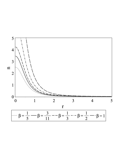
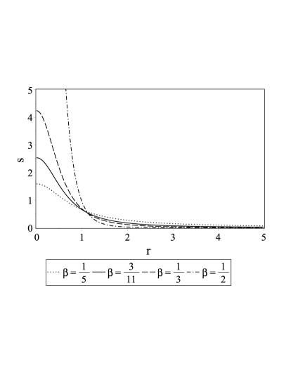
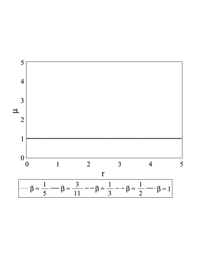
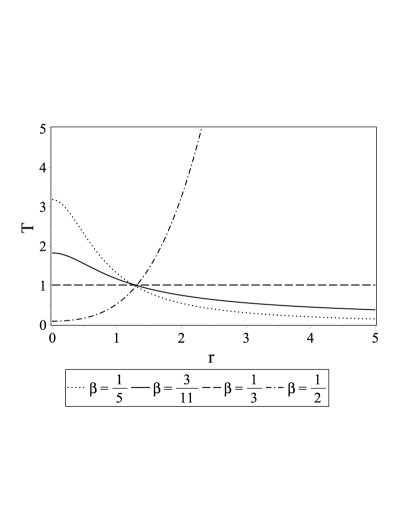
Figure 3: Thermodynamic quantities on the disk for different values of $\beta$. In the top part we show the particle number and entropy densities whilst in the bottom their corresponding conjugate quantities, chemical potential and temperature. The plots in the left are well behaved for any value of $\beta\in[1/5,1]$, the chemical potential is constant. The plots on the right are not defined for the case $\beta=1$. Moreover there are divergences for values of $\beta>1/3$. In all cases, the solid line represents the electromagnetic case we study. Here, we have used the values $a=1$ and $m=0.75$ [c.f. equation (12)].

A.C.G-P. is thankful to Departamento de Gravitación y Teoría de Campos (ICN-UNAM) for its hospitality and kind support though the course of his post-doctoral fellowship. He also wants to thank COLCIENCIAS, Colombia, and TWAS-CONACYT for financial support. CSLM acknowledges support from a UNAM-DGAPA postdoctoral grant. HQ receives partial support from CONACYT, Grant No. 166391 and DGAPA-UNAM. The authors would like to thank Francisco Nettel for useful comments and discussions.

Appendix A

For the metric (5) the non-zero components of the energy-momentum tensor of the halo as observed by a LSO are given by

$${M_{(0)(0)}^{\pm}} =-e^{2\beta\phi}\{-2\beta\nabla^{2}\phi+\beta^{2}\nabla\phi\cdot\nabla\phi+\frac{1}{2}e^{-2\phi}\nabla A_{0}\cdot\nabla A_{0}+\frac{1}{2}r^{-2}e^{2\beta\phi}\nabla A\cdot\nabla A\},$$ (30)

$${M_{(0)(1)}^{\pm}} =-r^{-1}e^{-(1-3\beta)\phi}\nabla A_{0}\cdot\nabla A,$$ (31)

$${M_{(1)(1)}^{\pm}} =e^{2\beta\phi}\{(1-\beta)\nabla^{2}{\phi}-(1-\beta)\frac{1}{r}\phi_{,r}+\nabla{\phi}\cdot\nabla{\phi}-\frac{1}{2}e^{-2\phi}\nabla A_{0}\cdot\nabla A_{0}-\frac{1}{2}r^{-2}e^{2\beta\phi}\nabla A\cdot\nabla A\},$$ (32)

$${M_{(2)(2)}^{\pm}} =e^{2\beta\phi}\{(1-\beta)\nabla^{2}{\phi}-(1-\beta)\phi_{,rr}+\phi_{,z}^{2}+(\beta^{2}-2\beta)\phi_{,r}^{2}+\frac{1}{2}e^{-2\phi}(A_{0,r}^{2}-A_{0,z}^{2})-\frac{1}{2}r^{-2}e^{2\beta\phi}(A_{,r}^{2}-A_{,z}^{2})\},$$ (33)

$${M_{(2)(3)}^{\pm}} =e^{2\beta\phi}\{(\beta-1)\phi_{,rz}+(\beta^{2}-2\beta-1)\phi_{,r}\phi_{,z}+e^{-2\phi}A_{0,r}A_{0,z}-r^{-2}e^{2\beta\phi}A_{,r}A_{,z}\},$$ (34)

$${M_{(3)(3)}^{\pm}} =e^{2\beta\phi}\{(1-\beta)\nabla^{2}{\phi}-(1-\beta)\phi_{,zz}+\phi_{,r}^{2}+(\beta^{2}-2\beta)\phi_{,z}^{2}-\frac{1}{2}e^{-2\phi}(A_{0,r}^{2}-A_{0,z}^{2})+\frac{1}{2}r^{-2}e^{2\beta\phi}(A_{,r}^{2}-A_{,z}^{2})\}.$$ (35)

References

- Bičák (2000) J. Bičák, in Einstein s field equations and their physical implications (Springer, 2000) pp. 1–126.
- Neugebauer and Meinel (1994) G. Neugebauer and R. Meinel, Physical Review Letters 73, 2166 (1994).
- González et al. (2008) G. A. González, A. C. Gutiérrez-Piñeres, and P. A. Ospina, Physical Review D 78, 064058 (2008), arXiv:0806.4285 [gr-qc] .
- González et al. (2009) G. A. González, A. C. Gutiérrez-Piñeres, and V. M. Viña-Cervantes, Physical Review D 79, 124048 (2009), arXiv:0811.3869 [gr-qc] .
- Gutiérrez-Piñeres et al. (2013) A. C. Gutiérrez-Piñeres, G. A. González, and H. Quevedo, Phys. Rev. D 87, 044010 (2013).
- Katz et al. (1999) J. Katz, J. Bicák, and D. Lynden-Bell, Classical and Quantum Gravity 16, 4023 (1999), arXiv:gr-qc/9910087 .
- Kuzmin (1956) G. Kuzmin, Astron. Zh 33, 27 (1956).
- Carter (1991) B. Carter, Royal Society of London Proceedings Series A 433, 45 (1991).
- Lopez-Monsalvo and Andersson (2011) C. S. Lopez-Monsalvo and N. Andersson, Royal Society of London Proceedings Series A 467, 738 (2011), arXiv:1006.2978 [gr-qc] .
- Samuelsson et al. (2010) L. Samuelsson, C. S. Lopez-Monsalvo, N. Andersson, and G. L. Comer, General Relativity and Gravitation 42, 413 (2010), arXiv:0906.4002 [gr-qc] .