On the largest Lyapunov exponent for products of Gaussian matrices

Vladislav Kargin
(Date: June 2014)
e-mail: vladislav.kargin@gmail.com

Abstract

The paper provides a new integral formula for the largest Lyapunov exponent of Gaussian matrices, which is valid in the real, complex and quaternion-valued cases. This formula is applied to derive asymptotic expressions for the largest Lyapunov exponent when the size of the matrix is large and compare the Lyapunov exponents in models with a spike and no spikes.


1. Introduction

Let Aksubscriptπ΄π‘˜A_{k} be random d𝑑d-by-d𝑑d matrices and let Pn:=An​Anβˆ’1​…​A1.assignsubscript𝑃𝑛subscript𝐴𝑛subscript𝐴𝑛1…subscript𝐴1P_{n}:=A_{n}A_{n-1}\ldots A_{1}. In a seminal paper [6], Furstenberg and Kesten showed that limnβ†’βˆžnβˆ’1​log⁑‖Pnβ€–subscript→𝑛superscript𝑛1normsubscript𝑃𝑛\lim_{n\rightarrow\infty}n^{-1}\log\left\|P_{n}\right\| exists under some mild conditions on random matrices Ak.subscriptπ΄π‘˜A_{k}. This limit is called the largest Lyapunov exponent. In fact, the limit of matrices (Pnβˆ—β€‹Pn)1/2​nsuperscriptsuperscriptsubscriptπ‘ƒπ‘›βˆ—subscript𝑃𝑛12𝑛\left(P_{n}^{\ast}P_{n}\right)^{1/2n} is well defined (under some conditions on Aksubscriptπ΄π‘˜A_{k}), and the limit has d𝑑d non-negative real eigenvalues (Oseledec [16], Raghunathan [19]). The logarithms of these eigenvalues are called the Lyapunov exponents of matrices Aisubscript𝐴𝑖A_{i}. We denote them ΞΌ1β‰₯…β‰₯ΞΌd.subscriptπœ‡1…subscriptπœ‡π‘‘\mu_{1}\geq\ldots\geq\mu_{d}.

As Lyapunov exponents are related to the behavior of complex dynamical systems, much research went into the study of their properties, such as their analyticity with respect to small matrix perturbations and to changes in the matrix random process ([20], [11], [17]), the multiplicity of the largest Lyapunov exponent ([8]), and others (see papers in [3]). Lyapunov exponents have been generalized to infinite-dimensional operators ([21], [10]), and found important applications in the study of hydrodynamic stability ([22]) and random Schroedinger operators ([2]).

In [7], Furstenberg derived an integral formula for the largest Lyapunov exponent, which in the case of Gaussian matrices reduces to a multidimensional integral over a known density. However, there is only a limited number of cases in which this integral has been computed in a closed form ([4], [13]), although in some cases, it was shown that the exponents can be computed efficiently even if one does non have an explicit formula ([18]).

Recently, in [5] Forrester found a formula for all Lyapunov exponents of complex Gaussian matrices with a general covariance matrix ΣΣ\Sigma. His method is based on the Harish-Chandra-Itzykson-Zuber integration formula and cannot be applied to the case when matrices are real-valued.

In this paper we derive a new formula for the largest Lyapunov exponent of Gaussian matrices with general ΣΣ\Sigma, which is applicable in the real, complex and quaternion cases.

Recall that a d𝑑d-by-d𝑑d Gaussian matrix A𝐴A with covariance matrix ΣΣ\Sigma has the probability density

P​(A)=cβ​(detΞ£)βˆ’d/2​exp⁑[βˆ’Ξ²2​Tr​(Aβˆ—β€‹Ξ£βˆ’1​A)],𝑃𝐴subscript𝑐𝛽superscriptΣ𝑑2𝛽2Trsuperscriptπ΄βˆ—superscriptΞ£1𝐴P\left(A\right)=c_{\beta}\left(\det\Sigma\right)^{-d/2}\exp\left[-\frac{\beta}{2}\mathrm{Tr}\left(A^{\ast}\Sigma^{-1}A\right)\right],

where Ξ²=1,𝛽1\beta=1, 2,22, or 444 for real, complex or quaternion matrices, and cΞ²subscript𝑐𝛽c_{\beta} is a normalization constant. Equivalently, A𝐴A can be defined as Ξ£1/2​G,superscriptΞ£12𝐺\Sigma^{1/2}G, where G𝐺G has independent real, complex, or quaternion entries whose components are real Gaussian variables with variance 1/Ξ²1𝛽1/\beta.

Theorem 1.1.

Let Aisubscript𝐴𝑖A_{i} be independent d𝑑d-by-d𝑑d Gaussian matrices with covariance matrixΒ Ξ£,Ξ£\Sigma, and let their entries be real, complex or quaternion, according to whether Ξ²=1,2,𝛽12\beta=1,2, or 4.44. Assume that the eigenvalues of ΣΣ\Sigma are Οƒi2=1/yi.superscriptsubscriptπœŽπ‘–21subscript𝑦𝑖\sigma_{i}^{2}=1/y_{i}. Then, the following formula holds for the largest Lyapunov exponent of Ai,subscript𝐴𝑖A_{i},

2​μ1=βˆ’Ξ³+log⁑(2Ξ²)+∫0∞[𝟏[0,1]​(x)βˆ’βˆi=1d(1+xyi)βˆ’Ξ²/2]​d​xx,2subscriptπœ‡1𝛾2𝛽superscriptsubscript0delimited-[]subscript101π‘₯superscriptsubscriptproduct𝑖1𝑑superscript1π‘₯subscript𝑦𝑖𝛽2𝑑π‘₯π‘₯2\mu_{1}=-\gamma+\log\left(\frac{2}{\beta}\right)+\int_{0}^{\infty}\left[\boldsymbol{1}_{[0,1]}\left(x\right)-\prod_{i=1}^{d}\left(1+\frac{x}{y_{i}}\right)^{-\beta/2}\right]\frac{dx}{x}, (1)

where Ξ³β‰ˆ0.5772𝛾0.5772\gamma\approx 0.5772 is the Euler constant.

As an application of this formula, we derive asymptotic expressions for the largest Lyapunov exponents of high-dimensional matrices. First, we compute the asymptotic behavior in the case when d𝑑d is large and ΣΣ\Sigma does not have spikes so that all eigenvalues of ΣΣ\Sigma are of the same order. Next, we consider the case when the covariance matrix ΣΣ\Sigma does have a β€œspike”. We consider the particular case when all except one eigenvalue of ΣΣ\Sigma equal 1/d1𝑑1/d, and the exceptional eigenvalue does not depend on the dimension. We study the asymptotic behavior of the largest Lyapunov exponent when the dimension d𝑑d is large, and find a significant difference relative to the case of no spikes.

More formally, we have the following result for the no-spike case.

Theorem 1.2.

Suppose that Ai(d)superscriptsubscript𝐴𝑖𝑑A_{i}^{\left(d\right)} are independent d𝑑d-by-d𝑑d Gaussian matrices with covariance matrix Ξ£d,subscriptΣ𝑑\Sigma_{d}, and let the eigenvalues of Ξ£dsubscriptΣ𝑑\Sigma_{d} be ΞΈi(d)/dsuperscriptsubscriptπœƒπ‘–π‘‘π‘‘\theta_{i}^{\left(d\right)}/d where i=1,…,d.𝑖1…𝑑i=1,\ldots,d. Assume that ΞΈi(d)superscriptsubscriptπœƒπ‘–π‘‘\theta_{i}^{\left(d\right)} are bounded, 1≀θi(d)≀L,1superscriptsubscriptπœƒπ‘–π‘‘πΏ1\leq\theta_{i}^{\left(d\right)}\leq L, and that

limdβ†’βˆžTr​(Ξ£d)≑limdβ†’βˆž1dβ€‹βˆ‘i=1dΞΈi(d)=Ξ».subscript→𝑑TrsubscriptΣ𝑑subscript→𝑑1𝑑superscriptsubscript𝑖1𝑑superscriptsubscriptπœƒπ‘–π‘‘πœ†\lim_{d\rightarrow\infty}\mathrm{Tr}\left(\Sigma_{d}\right)\equiv\lim_{d\rightarrow\infty}\frac{1}{d}\sum_{i=1}^{d}\theta_{i}^{\left(d\right)}=\lambda.

Then, for the largest Lyapunov exponent of Ai(d),superscriptsubscript𝐴𝑖𝑑A_{i}^{\left(d\right)}, we have

limdβ†’βˆžΞΌ1(d)=12​log⁑λ.subscript→𝑑superscriptsubscriptπœ‡1𝑑12πœ†\lim_{d\rightarrow\infty}\mu_{1}^{\left(d\right)}=\frac{1}{2}\log\lambda.

The result of Theorem 1.2 is in agreement with the free probability prediction (see, for example, [9]).
Refer to caption
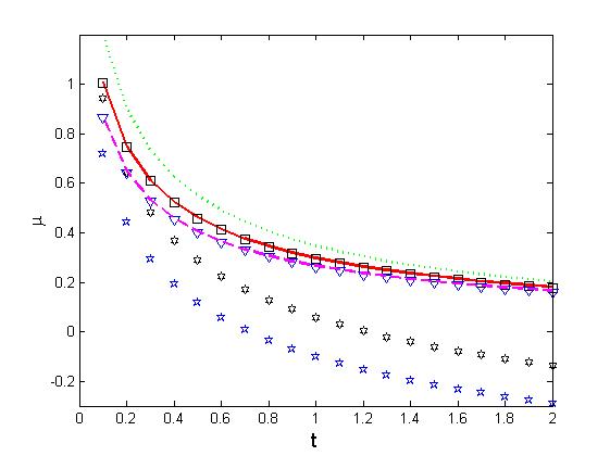
Figure 1. The eigenvalues of the covariance matrix equal 1/d1𝑑1/d except one which equals 1/t1𝑑1/t. The blue pentagrams show the largest Lyapunov exponents when the dimension d=2𝑑2d=2 and Ξ²=1𝛽1\beta=1; the black hexagrams are for d=2𝑑2d=2 and Ξ²=2𝛽2\beta=2; the triangles are for d=100𝑑100d=100 and Ξ²=1𝛽1\beta=1; the squares are for d=100𝑑100d=100 and Ξ²=2𝛽2\beta=2; the red solid line is the asymptotic prediction for Ξ²=2𝛽2\beta=2 and the magenta dashed line is the prediction for Ξ²=1𝛽1\beta=1; the green dotted line is the free probability prediction log⁑(1+1/t)/211𝑑2\log(1+1/t)/2.

For the model with a spike we have the following result.

Theorem 1.3.

Suppose that Aisubscript𝐴𝑖A_{i} are independent d𝑑d-by-d𝑑d Gaussian matrices with the covariance matrix Ξ£d,subscriptΣ𝑑\Sigma_{d}, and that the eigenvalues of Ξ£dsubscriptΣ𝑑\Sigma_{d} are Ξ»i(d)=1/dsuperscriptsubscriptπœ†π‘–π‘‘1𝑑\lambda_{i}^{\left(d\right)}=1/d for i=1,…,dβˆ’1,𝑖1…𝑑1i=1,\ldots,d-1, and Ξ»d(d)=1/tsuperscriptsubscriptπœ†π‘‘π‘‘1𝑑\lambda_{d}^{\left(d\right)}=1/t, where 0<t<d.0𝑑𝑑0<t<d. In the complex case (Ξ²=2𝛽2\beta=2), we have the following estimate,

2​μ12subscriptπœ‡1\displaystyle 2\mu_{1} =\displaystyle= etβ€‹βˆ«1∞eβˆ’t​x​d​xx+Ot​(1/d),superscript𝑒𝑑superscriptsubscript1superscript𝑒𝑑π‘₯𝑑π‘₯π‘₯subscript𝑂𝑑1𝑑\displaystyle e^{t}\int_{1}^{\infty}e^{-tx}\frac{dx}{x}+O_{t}\left(1/d\right),
=\displaystyle= βˆ’et​Ei​(βˆ’t)+Ot​(1/d),superscript𝑒𝑑Ei𝑑subscript𝑂𝑑1𝑑\displaystyle-e^{t}\mathrm{Ei}\left(-t\right)+O_{t}\left(1/d\right),

where Ei​(x)Eiπ‘₯\mathrm{Ei}\left(x\right) is the exponential integral function. In the real case (Ξ²=1𝛽1\beta=1),

2​μ1=et/2β€‹βˆ«1∞eβˆ’t​x/2​d​xx​(x+1)+Ot​(1/d),2subscriptπœ‡1superscript𝑒𝑑2superscriptsubscript1superscript𝑒𝑑π‘₯2𝑑π‘₯π‘₯π‘₯1subscript𝑂𝑑1𝑑2\mu_{1}=e^{t/2}\int_{1}^{\infty}e^{-tx/2}\frac{dx}{\sqrt{x}\left(\sqrt{x}+1\right)}+O_{t}\left(1/d\right),

A comparison of the results for the spike and no-spike models shows that a spike can significantly influence the largest Lyapunov exponent. Indeed, in the situation of Theorem 1.3 with Ξ²=2𝛽2\beta=2, the formula in Theorem 1.2 would incorrectly predict that for large d𝑑d the first Lyapunov exponent is close to 12​log⁑(1+1/t)1211𝑑\frac{1}{2}\log(1+1/t) (because limdβ†’βˆž1dβ€‹βˆ‘i=1dΞΈi(d)=1+1tsubscript→𝑑1𝑑superscriptsubscript𝑖1𝑑superscriptsubscriptπœƒπ‘–π‘‘11𝑑\lim_{d\rightarrow\infty}\frac{1}{d}\sum_{i=1}^{d}\theta_{i}^{\left(d\right)}=1+\frac{1}{t}) instead of the correct βˆ’12​et​Ei​(βˆ’t)12superscript𝑒𝑑Ei𝑑-\frac{1}{2}e^{t}\mathrm{Ei}\left(-t\right).

Theorem 1.3 concerns the case when the spike (i.e., the ratio of the exceptional eigenvalue to the bulk eigenvalues) grows at the same rate as the dimension. For other regimes, we have the following results.

Theorem 1.4.

Suppose that Aisubscript𝐴𝑖A_{i} are independent d𝑑d-by-d𝑑d complex Gaussian matrices with the covariance Ξ£,Ξ£\Sigma, and that the eigenvalues of Ξ£dsubscriptΣ𝑑\Sigma_{d} are Ξ»i(d)=1/dsuperscriptsubscriptπœ†π‘–π‘‘1𝑑\lambda_{i}^{\left(d\right)}=1/d for i=1,…,dβˆ’1,𝑖1…𝑑1i=1,\ldots,d-1, and Ξ»d(d)=ΞΈ/dsuperscriptsubscriptπœ†π‘‘π‘‘πœƒπ‘‘\lambda_{d}^{\left(d\right)}=\theta/d, where ΞΈ>1.πœƒ1\theta>1. Then, for the largest Lyapunov exponent ΞΌ1,subscriptπœ‡1\mu_{1}, we have

2​μ1=ΞΈβˆ’32d+O​((ΞΈβˆ’1d)2)+O​(1d2).2subscriptπœ‡1πœƒ32𝑑𝑂superscriptπœƒ1𝑑2𝑂1superscript𝑑22\mu_{1}=\frac{\theta-\frac{3}{2}}{d}+O\left(\left(\frac{\theta-1}{d}\right)^{2}\right)+O\left(\frac{1}{d^{2}}\right).

Note that for dβ†’βˆžβ†’π‘‘d\rightarrow\infty and ΞΈπœƒ\theta fixed, this is essentially the no-spike model with Ξ»=limdβ†’βˆž1dβ€‹βˆ‘i=1dΞΈi(d)=1.πœ†subscript→𝑑1𝑑superscriptsubscript𝑖1𝑑superscriptsubscriptπœƒπ‘–π‘‘1\lambda=\lim_{d\rightarrow\infty}\frac{1}{d}\sum_{i=1}^{d}\theta_{i}^{\left(d\right)}=1. Thus, Theorem 1.4 gives a second order correction to the result in Theorem 1.2.

Finally, consider the case of an exceptionally large eigenvalue which grows faster than the dimension d.𝑑d.

Theorem 1.5.

Suppose that Aisubscript𝐴𝑖A_{i} are independent d𝑑d-by-d𝑑d complex Gaussian matrices with the covariance Ξ£,Ξ£\Sigma, and that the eigenvalues of Ξ£dsubscriptΣ𝑑\Sigma_{d} are Ξ»i(d)=1superscriptsubscriptπœ†π‘–π‘‘1\lambda_{i}^{\left(d\right)}=1 for i=1,…,dβˆ’1,𝑖1…𝑑1i=1,\ldots,d-1, and Ξ»d(d)=ΞΈ>d.superscriptsubscriptπœ†π‘‘π‘‘πœƒπ‘‘\lambda_{d}^{\left(d\right)}=\theta>d. Then, for the largest Lyapunov exponent ΞΌ1,subscriptπœ‡1\mu_{1}, we have

2​μ1=logβ‘ΞΈβˆ’Ξ³+O​(dθ​log⁑θ).2subscriptπœ‡1πœƒπ›Ύπ‘‚π‘‘πœƒπœƒ2\mu_{1}=\log\theta-\gamma+O(\frac{d}{\theta}\log\theta).

In particular, if ΞΈπœƒ\theta grows faster than dΞ±superscript𝑑𝛼d^{\alpha} with Ξ±>1,𝛼1\alpha>1, then the last term is negligible for large ΞΈ.πœƒ\theta. This happens, for example, if d𝑑d is fixed and ΞΈπœƒ\theta grows. It is remarkable that the Lyapunov exponent does not depend on the dimension d𝑑d if the spike in covariance ΞΈπœƒ\theta is much larger than d𝑑d.

The rest of the paper is organized as follows. Section 2 collects necessary background information about Lyapunov exponents. Section 3 is devoted to the proof of the main formula. Section 4 derives asymptotic expressions for the largest Lyapunov exponent when the size of the matrices is large. And Section 5 is the conclusion.

2. Background information about Lyapunov exponents

One of the key facts about Lyapunov exponents is that they satisfy the following relation:

ΞΌ1+…+ΞΌk=limnβ†’βˆž1n​log⁑Volk​(y1​(n),…,yk​(n))subscriptπœ‡1…subscriptπœ‡π‘˜subscript→𝑛1𝑛subscriptVolπ‘˜subscript𝑦1𝑛…subscriptπ‘¦π‘˜π‘›\mu_{1}+\ldots+\mu_{k}=\lim_{n\rightarrow\infty}\frac{1}{n}\log\mathrm{Vol}_{k}\left(y_{1}\left(n\right),\ldots,y_{k}\left(n\right)\right) (3)

where yi​(n)=Pn​yi​(0)subscript𝑦𝑖𝑛subscript𝑃𝑛subscript𝑦𝑖0y_{i}\left(n\right)=P_{n}y_{i}\left(0\right) and {yi​(0)}i=1ksuperscriptsubscriptsubscript𝑦𝑖0𝑖1π‘˜\left\{y_{i}\left(0\right)\right\}_{i=1}^{k} is an arbitrary orthonormal vector system.

For Gaussian matrices this formula can be significantly simplified. Namely, let Aisubscript𝐴𝑖A_{i} be independent Gaussian matrices with covariance matrixΒ Ξ£.Ξ£\Sigma. The crucial observation is that the distribution of Aiβˆ—β€‹Aisuperscriptsubscriptπ΄π‘–βˆ—subscript𝐴𝑖A_{i}^{\ast}A_{i} is invariant relative to the transformation

Aiβˆ—β€‹Aiβ†’Qβˆ—β€‹Aiβˆ—β€‹Ai​Q,β†’superscriptsubscriptπ΄π‘–βˆ—subscript𝐴𝑖superscriptπ‘„βˆ—superscriptsubscriptπ΄π‘–βˆ—subscript𝐴𝑖𝑄A_{i}^{\ast}A_{i}\rightarrow Q^{\ast}A_{i}^{\ast}A_{i}Q,

where Q𝑄Q is an arbitrary orthogonal matrix. This implies that the changes in the volume of a kπ‘˜k-dimensional element are independent from step to step and that their distribution is the same as if they were applied to the element spanned by the standard basis vectors 𝐞i.subscriptπžπ‘–\mathbf{e}_{i}. Hence, by the law of large numbers,

ΞΌ1+…+ΞΌksubscriptπœ‡1…subscriptπœ‡π‘˜\displaystyle\mu_{1}+\ldots+\mu_{k} =\displaystyle= 𝔼​log⁑Volk​(A1β€‹πž1,…,A1β€‹πžk)𝔼subscriptVolπ‘˜subscript𝐴1subscript𝐞1…subscript𝐴1subscriptπžπ‘˜\displaystyle\mathbb{E}\log\mathrm{Vol}_{k}\left(A_{1}\mathbf{e}_{1},\ldots,A_{1}\mathbf{e}_{k}\right) (4)
=\displaystyle= 12​𝔼​log​det(Gkβˆ—β€‹Ξ£β€‹Gk)=12​dd​μ​𝔼​[det(Gkβˆ—β€‹Ξ£β€‹Gk)ΞΌ]|ΞΌ=0,12𝔼superscriptsubscriptπΊπ‘˜βˆ—Ξ£subscriptπΊπ‘˜evaluated-at12π‘‘π‘‘πœ‡π”Όdelimited-[]superscriptsuperscriptsubscriptπΊπ‘˜βˆ—Ξ£subscriptπΊπ‘˜πœ‡πœ‡0\displaystyle\frac{1}{2}\mathbb{E}\log\det\left(G_{k}^{\ast}\Sigma G_{k}\right)=\frac{1}{2}\left.\frac{d}{d\mu}\mathbb{E}\left[\det\left(G_{k}^{\ast}\Sigma G_{k}\right)^{\mu}\right]\right|_{\mu=0},

where GksubscriptπΊπ‘˜G_{k} denotes a random d𝑑d-by-kπ‘˜k matrix with the identically distributed standard Gaussian entries. (For details of the argument see [14] and [15].)

While formula (4) allows one to compute all Lyapunov exponents, it is essentially a multidimensional integral which can be computationally demanding. For this reason, it is of interest to obtain a more explicit way to calculate the Lyapunov exponents.

For real Gaussian matrices and the simplest situation when Ξ£=Οƒ2​IΞ£superscript𝜎2𝐼\Sigma=\sigma^{2}I and I𝐼I is the identity matrix, Newman showed in [15] that

ΞΌi=12​[log⁑(2​σ2)+Ψ​(dβˆ’i+12)],subscriptπœ‡π‘–12delimited-[]2superscript𝜎2Ψ𝑑𝑖12\mu_{i}=\frac{1}{2}\left[\log\left(2\sigma^{2}\right)+\Psi\left(\frac{d-i+1}{2}\right)\right], (5)

where Ψ​(x)Ξ¨π‘₯\Psi\left(x\right) is the digamma function, Ψ​(x):=(log⁑Γ​(x))β€².assignΞ¨π‘₯superscriptΞ“π‘₯β€²\Psi\left(x\right):=\left(\log\Gamma\left(x\right)\right)^{\prime}. (At the positive integer points, Ψ​(n)=βˆ‘k=1nβˆ’11kβˆ’Ξ³,Ψ𝑛superscriptsubscriptπ‘˜1𝑛11π‘˜π›Ύ\Psi\left(n\right)=\sum_{k=1}^{n-1}\frac{1}{k}-\gamma, where Ξ³=0.5772​…𝛾0.5772…\gamma=0.5772\ldots is the Euler constant. At half-integers, Ψ​(n+1/2)=βˆ‘k=1n1kβˆ’1/2βˆ’2​log⁑2βˆ’Ξ³.Ψ𝑛12superscriptsubscriptπ‘˜1𝑛1π‘˜1222𝛾\Psi\left(n+1/2\right)=\sum_{k=1}^{n}\frac{1}{k-1/2}-2\log 2-\gamma. The asymptotic behavior of the digamma function is given by the formula Ψ​(z)=log⁑zβˆ’12​zβˆ’112​z2​(1+O​(1z2))Ψ𝑧𝑧12𝑧112superscript𝑧21𝑂1superscript𝑧2\Psi\left(z\right)=\log z-\frac{1}{2z}-\frac{1}{12z^{2}}\left(1+O\left(\frac{1}{z^{2}}\right)\right).)

In particular if we normalize Οƒ2=1/d,superscript𝜎21𝑑\sigma^{2}=1/d, then for d=1𝑑1d=1 the largest Lyapunov exponent ΞΌ1=[βˆ’log⁑2βˆ’Ξ³]/2subscriptπœ‡1delimited-[]2𝛾2\mu_{1}=[-\log 2-\gamma]/2 and for dβ†’βˆž,→𝑑d\rightarrow\infty, ΞΌ1=βˆ’12​d+O​(1d2).subscriptπœ‡112𝑑𝑂1superscript𝑑2\mu_{1}=-\frac{1}{2d}+O\left(\frac{1}{d^{2}}\right).

In [5], Forrester established an analogue of formulas (5) for the complex-valued Gaussian matrices. Namely, Forrester showed that in the case of complex-valued Gaussian matrices with Ξ£=Οƒ2​IΞ£superscript𝜎2𝐼\Sigma=\sigma^{2}I,

2​μi=log⁑σ2+Ψ​(dβˆ’i+1)2subscriptπœ‡π‘–superscript𝜎2Ψ𝑑𝑖12\mu_{i}=\log\sigma^{2}+\Psi\left(d-i+1\right) (6)

(see Proposition 1 in [5] and note that the absence of 1/2121/2 before ΨΨ\Psi is a typo in the statement of this proposition.) If Οƒ2=1/d,superscript𝜎21𝑑\sigma^{2}=1/d, then for d=1𝑑1d=1 the largest Lyapunov exponent ΞΌ1=βˆ’Ξ³/2subscriptπœ‡1𝛾2\mu_{1}=-\gamma/2 and for dβ†’βˆž,→𝑑d\rightarrow\infty, ΞΌ1=βˆ’14​d+O​(1d2).subscriptπœ‡114𝑑𝑂1superscript𝑑2\mu_{1}=-\frac{1}{4d}+O\left(\frac{1}{d^{2}}\right).

What is more, in the complex-valued case there is an explicit formula for all Lyapunov exponents even if ΣΣ\Sigma is general. Namely, it is shown in [5] that

ΞΌk=12​Ψ​(k)+12β€‹βˆi<j(yiβˆ’yj)​det[[yjiβˆ’1]i=1,…,kβˆ’1;j=1,…,d[(log⁑yj)​yjkβˆ’1]j=1,…,d[yjiβˆ’1]i=k+1,…,d;j=1,…,d],subscriptπœ‡π‘˜12Ξ¨π‘˜12subscriptproduct𝑖𝑗subscript𝑦𝑖subscript𝑦𝑗delimited-[]subscriptdelimited-[]superscriptsubscript𝑦𝑗𝑖1formulae-sequence𝑖1β€¦π‘˜1𝑗1…𝑑subscriptdelimited-[]subscript𝑦𝑗superscriptsubscriptπ‘¦π‘—π‘˜1𝑗1…𝑑subscriptdelimited-[]superscriptsubscript𝑦𝑗𝑖1formulae-sequenceπ‘–π‘˜1…𝑑𝑗1…𝑑\mu_{k}=\frac{1}{2}\Psi\left(k\right)+\frac{1}{2\prod\limits_{i<j}\left(y_{i}-y_{j}\right)}\det\left[\begin{array}[]{c}\left[y_{j}^{i-1}\right]_{i=1,\ldots,k-1;j=1,\ldots,d}\\ \left[\left(\log y_{j}\right)y_{j}^{k-1}\right]_{j=1,\ldots,d}\\ \left[y_{j}^{i-1}\right]_{i=k+1,\ldots,d;j=1,\ldots,d}\end{array}\right], (7)

where yjsubscript𝑦𝑗y_{j} are eigenvalues of Ξ£βˆ’1.superscriptΞ£1\Sigma^{-1}. In particular for k=1,π‘˜1k=1, one can re-write this as

ΞΌ1=12​[Ψ​(1)βˆ’βˆ‘j=1dlog⁑yj∏lβ‰ j(1βˆ’yj/yl)]subscriptπœ‡112delimited-[]Ξ¨1superscriptsubscript𝑗1𝑑subscript𝑦𝑗subscriptproduct𝑙𝑗1subscript𝑦𝑗subscript𝑦𝑙\mu_{1}=\frac{1}{2}\left[\Psi\left(1\right)-\sum_{j=1}^{d}\frac{\log y_{j}}{\prod_{l\neq j}\left(1-y_{j}/y_{l}\right)}\right] (8)

provided that all yjsubscript𝑦𝑗y_{j} are different.

The proof of formula (7) is based on the Harish-Chandra-Itzykson-Zuber integral and cannot be directly generalized to the case of real or quaternion Gaussian matrices.

In fact, it appears that for the real-valued case with general Ξ£,Ξ£\Sigma, an explicit formula (due to Mannion [12]) is only known for products of 2-by-2 Gaussian matrices:

ΞΌ1=12​[Ψ​(1)+log⁑(12​Tr​Σ+detΞ£)].subscriptπœ‡112delimited-[]Ξ¨112TrΣΣ\mu_{1}=\frac{1}{2}\left[\Psi\left(1\right)+\log\left(\frac{1}{2}\mathrm{Tr}\Sigma+\sqrt{\det\Sigma}\right)\right]. (9)

(Some explicit formulas are also known for 2-by-2 random matrices with non-Gaussian entries, see [13]. In addition, there are methods which sometime allow one to compute Lyapunov exponents efficiently even when explicit formulas are not available, see [18].)

Our formula (1) in Theorem 1.1 provides an explicit formula applicable for real, complex and quaternion matrices with general ΣΣ\Sigma. It is limited, however, to the case of the largest Lyapunov exponent. For Ξ²=2,𝛽2\beta=2, Forrester’s formula (8) can be derived from our formula by evaluating the integral in (1) using residues. Similarly, for Ξ²=4,𝛽4\beta=4, one can use residues and derive the following formula:

2​μ12subscriptπœ‡1\displaystyle 2\mu_{1} =\displaystyle= Ψ​(1)βˆ’log⁑(2)Ξ¨12\displaystyle\Psi\left(1\right)-\log\left(2\right)
βˆ’(∏i=1dyi)2β€‹βˆ‘i=1d{1yi2β€‹βˆjβ‰ i(yiβˆ’yj)2​[1βˆ’log⁑yi​(1+βˆ‘jβ‰ i2​yiyiβˆ’yj)]}.superscriptsuperscriptsubscriptproduct𝑖1𝑑subscript𝑦𝑖2superscriptsubscript𝑖1𝑑1superscriptsubscript𝑦𝑖2subscriptproduct𝑗𝑖superscriptsubscript𝑦𝑖subscript𝑦𝑗2delimited-[]1subscript𝑦𝑖1subscript𝑗𝑖2subscript𝑦𝑖subscript𝑦𝑖subscript𝑦𝑗\displaystyle-\left(\prod\limits_{i=1}^{d}y_{i}\right)^{2}\sum_{i=1}^{d}\left\{\frac{1}{y_{i}^{2}\prod\limits_{j\neq i}\left(y_{i}-y_{j}\right)^{2}}\left[1-\log y_{i}\left(1+\sum_{j\neq i}\frac{2y_{i}}{y_{i}-y_{j}}\right)\right]\right\}.

In the remaining case of Ξ²=1,𝛽1\beta=1, the integral can be easily evaluated numerically. In the asymptotic analysis of large-dimensional situations, we will use our formula (1) as most convenient even for Ξ²=2𝛽2\beta=2 and 4.44.

3. Proof of the formula for the largest Lyapunov exponent

We start the proof of Theorem 1.1 by interpreting the basic formula (4) for k=1.π‘˜1k=1. Namely, by (4), ΞΌ1subscriptπœ‡1\mu_{1} is the expected logarithm of β€–Ξ£1/2​G1β€–normsuperscriptΞ£12subscript𝐺1\left\|\Sigma^{1/2}G_{1}\right\|. Since β€–Ξ£1/2​G1β€–2superscriptnormsuperscriptΞ£12subscript𝐺12\left\|\Sigma^{1/2}G_{1}\right\|^{2} is a weighted sum of the squares of independent Gaussian variables, its distribution is easy to calculate. Indeed, in the real case Ξ²=1,𝛽1\beta=1, the characteristic function of the sum is

f​(t)=∏j=1d(1βˆ’2​i​σj2​t)βˆ’1/2.𝑓𝑑superscriptsubscriptproduct𝑗1𝑑superscript12𝑖superscriptsubscriptπœŽπ‘—2𝑑12f\left(t\right)=\prod_{j=1}^{d}\left(1-2i\sigma_{j}^{2}t\right)^{-1/2}.

(In this formula, the function zβˆ’1/2superscript𝑧12z^{-1/2} is determined by making a cut along z<0,𝑧0z<0, and the selected branch of (1βˆ’2​i​σj2​t)βˆ’1/2superscript12𝑖superscriptsubscriptπœŽπ‘—2𝑑12\left(1-2i\sigma_{j}^{2}t\right)^{-1/2} equals 111 at t=0.𝑑0t=0.) Hence, the distribution density of the sum is

p​(Ξ»)π‘πœ†\displaystyle p\left(\lambda\right) =\displaystyle= 12β€‹Ο€β€‹βˆ«βˆ’βˆžβˆžeβˆ’i​λ​tβ€‹βˆj=1d(1βˆ’2​i​σj2​t)βˆ’1/2​d​t12πœ‹superscriptsubscriptsuperscriptπ‘’π‘–πœ†π‘‘superscriptsubscriptproduct𝑗1𝑑superscript12𝑖superscriptsubscriptπœŽπ‘—2𝑑12𝑑𝑑\displaystyle\frac{1}{2\pi}\int_{-\infty}^{\infty}e^{-i\lambda t}\prod_{j=1}^{d}\left(1-2i\sigma_{j}^{2}t\right)^{-1/2}dt
=\displaystyle= 12​π​(Ξ j=1d​yj)1/2β€‹βˆ«βˆ’βˆžβˆžeβˆ’i​λ​tβ€‹βˆj=1d(yjβˆ’2​i​t)βˆ’1/2​d​t12πœ‹superscriptsuperscriptsubscriptΠ𝑗1𝑑subscript𝑦𝑗12superscriptsubscriptsuperscriptπ‘’π‘–πœ†π‘‘superscriptsubscriptproduct𝑗1𝑑superscriptsubscript𝑦𝑗2𝑖𝑑12𝑑𝑑\displaystyle\frac{1}{2\pi}\left(\Pi_{j=1}^{d}y_{j}\right)^{1/2}\int_{-\infty}^{\infty}e^{-i\lambda t}\prod_{j=1}^{d}\left(y_{j}-2it\right)^{-1/2}dt
=\displaystyle= cβ€‹βˆ«0+iβ€‹βˆž0βˆ’iβ€‹βˆžeβˆ’Ξ»β€‹z/2β€‹βˆi=1d(zβˆ’yi)βˆ’1/2​d​z,𝑐superscriptsubscript0𝑖0𝑖superscriptπ‘’πœ†π‘§2superscriptsubscriptproduct𝑖1𝑑superscript𝑧subscript𝑦𝑖12𝑑𝑧\displaystyle c\int_{0\mathcal{+}i\infty}^{0-i\infty}e^{-\lambda z/2}\prod_{i=1}^{d}\left(z-y_{i}\right)^{-1/2}dz,

where yi=1/Οƒi2subscript𝑦𝑖1superscriptsubscriptπœŽπ‘–2y_{i}=1/\sigma_{i}^{2} and the normalization constant c𝑐c may depend on yisubscript𝑦𝑖y_{i} and the choice of branch for functions (zβˆ’yi)βˆ’1/2.superscript𝑧subscript𝑦𝑖12\left(z-y_{i}\right)^{-1/2}. By changing the contour, we get the expression

p​(Ξ»)=1cβ€‹βˆ«π’žeβˆ’Ξ»β€‹z/2β€‹βˆi=1d(zβˆ’yi)βˆ’1/2​d​z,π‘πœ†1𝑐subscriptπ’žsuperscriptπ‘’πœ†π‘§2superscriptsubscriptproduct𝑖1𝑑superscript𝑧subscript𝑦𝑖12𝑑𝑧p\left(\lambda\right)=\frac{1}{c}\int_{\mathcal{C}}e^{-\lambda z/2}\prod_{i=1}^{d}\left(z-y_{i}\right)^{-1/2}dz,

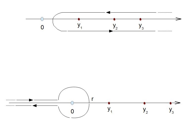
and the contour of integration goes in the counterclockwise direction around points yi.subscript𝑦𝑖y_{i}. In more detail, we can take the contour π’žπ’ž\mathcal{C} that starts at a large R>max⁑{yi},𝑅subscript𝑦𝑖R>\max\left\{y_{i}\right\}, goes along the upper edge of the real axis to r>0,π‘Ÿ0r>0, which is smaller than all of yi,subscript𝑦𝑖y_{i}, then crosses to the lower edge of the real axis, and then returns along this lower edge to R.𝑅R. We then take the limit for Rβ†’βˆž.→𝑅R\rightarrow\infty.

For general β𝛽\beta (i.e., Ξ²=1,2,𝛽12\beta=1,2, or 444), we can similarly obtain

pβ​(Ξ»)=1cΞ²β€‹βˆ«π’žeβˆ’Ξ²β€‹Ξ»β€‹z/2β€‹βˆi=1d(zβˆ’yi)βˆ’Ξ²/2​d​z.subscriptπ‘π›½πœ†1subscript𝑐𝛽subscriptπ’žsuperscriptπ‘’π›½πœ†π‘§2superscriptsubscriptproduct𝑖1𝑑superscript𝑧subscript𝑦𝑖𝛽2𝑑𝑧p_{\beta}\left(\lambda\right)=\frac{1}{c_{\beta}}\int_{\mathcal{C}}e^{-\beta\lambda z/2}\prod_{i=1}^{d}\left(z-y_{i}\right)^{-\beta/2}dz.

Next, we use formula (4) and find that

ΞΌ1=12​cΞ²β€‹βˆ«0∞log⁑λ​[βˆ«π’žeβˆ’Ξ²β€‹Ξ»β€‹z/2β€‹βˆi=1d(zβˆ’yi)βˆ’Ξ²/2​d​z]​𝑑λ,subscriptπœ‡112subscript𝑐𝛽superscriptsubscript0πœ†delimited-[]subscriptπ’žsuperscriptπ‘’π›½πœ†π‘§2superscriptsubscriptproduct𝑖1𝑑superscript𝑧subscript𝑦𝑖𝛽2𝑑𝑧differential-dπœ†\mu_{1}=\frac{1}{2c_{\beta}}\int_{0}^{\infty}\log\lambda\left[\int_{\mathcal{C}}e^{-\beta\lambda z/2}\prod_{i=1}^{d}\left(z-y_{i}\right)^{-\beta/2}dz\right]d\lambda, (11)

where

cΞ²=∫0βˆžβˆ«π’žeβˆ’Ξ²β€‹Ξ»β€‹z/2β€‹βˆi=1d(zβˆ’yi)βˆ’Ξ²/2​d​z​d​λ.subscript𝑐𝛽superscriptsubscript0subscriptπ’žsuperscriptπ‘’π›½πœ†π‘§2superscriptsubscriptproduct𝑖1𝑑superscript𝑧subscript𝑦𝑖𝛽2π‘‘π‘§π‘‘πœ†c_{\beta}=\int_{0}^{\infty}\int_{\mathcal{C}}e^{-\beta\lambda z/2}\prod_{i=1}^{d}\left(z-y_{i}\right)^{-\beta/2}dzd\lambda. (12)

By changing the order of integration in (11) and computing the inner integral, we find (with the help of the identity ∫0∞(log⁑t)​eβˆ’t​𝑑t=βˆ’Ξ³superscriptsubscript0𝑑superscript𝑒𝑑differential-d𝑑𝛾\int_{0}^{\infty}\left(\log t\right)e^{-t}dt=-\gamma) that

2​μ1=βˆ’Ξ³+1c~β​[12​π​iβ€‹βˆ«π’ž(2β​z)​log⁑(2β​z)β€‹βˆi=1d(zβˆ’yi)βˆ’Ξ²/2​d​z],2subscriptπœ‡1𝛾1subscript~𝑐𝛽delimited-[]12πœ‹π‘–subscriptπ’ž2𝛽𝑧2𝛽𝑧superscriptsubscriptproduct𝑖1𝑑superscript𝑧subscript𝑦𝑖𝛽2𝑑𝑧2\mu_{1}=-\gamma+\frac{1}{\widetilde{c}_{\beta}}\left[\frac{1}{2\pi i}\int_{\mathcal{C}}\left(\frac{2}{\beta z}\right)\log\left(\frac{2}{\beta z}\right)\prod_{i=1}^{d}\left(z-y_{i}\right)^{-\beta/2}dz\right], (13)

where

c~Ξ²subscript~𝑐𝛽\displaystyle\widetilde{c}_{\beta} =\displaystyle= cΞ²2​π​i=12​π​iβ€‹βˆ«π’ž(2β​z)β€‹βˆi=1d(zβˆ’yi)βˆ’Ξ²/2​d​zsubscript𝑐𝛽2πœ‹π‘–12πœ‹π‘–subscriptπ’ž2𝛽𝑧superscriptsubscriptproduct𝑖1𝑑superscript𝑧subscript𝑦𝑖𝛽2𝑑𝑧\displaystyle\frac{c_{\beta}}{2\pi i}=\frac{1}{2\pi i}\int_{\mathcal{C}}\left(\frac{2}{\beta z}\right)\prod_{i=1}^{d}\left(z-y_{i}\right)^{-\beta/2}dz
=\displaystyle= 2Ξ²β€‹βˆi=1d(βˆ’yi)βˆ’Ξ²/2.2𝛽superscriptsubscriptproduct𝑖1𝑑superscriptsubscript𝑦𝑖𝛽2\displaystyle\frac{2}{\beta}\prod\limits_{i=1}^{d}\left(-y_{i}\right)^{-\beta/2}.

This implies that

2​μ1=Ψ​(1)+log⁑(2Ξ²)+12​π​iβ€‹βˆ«π’žlog⁑(z)β€‹βˆi=1d(1βˆ’zyi)βˆ’Ξ²/2​d​zz.2subscriptπœ‡1Ξ¨12𝛽12πœ‹π‘–subscriptπ’žπ‘§superscriptsubscriptproduct𝑖1𝑑superscript1𝑧subscript𝑦𝑖𝛽2𝑑𝑧𝑧2\mu_{1}=\Psi\left(1\right)+\log\left(\frac{2}{\beta}\right)+\frac{1}{2\pi i}\int_{\mathcal{C}}\log\left(z\right)\prod_{i=1}^{d}\left(1-\frac{z}{y_{i}}\right)^{-\beta/2}\frac{dz}{z}. (14)
Refer to caption
Figure 2. Original and modified contours.

Now, let us change the contour. As before, let the contour start at a large R>max⁑{yi},𝑅subscript𝑦𝑖R>\max\left\{y_{i}\right\}, goes along the upper edge of the real axis to r>0,π‘Ÿ0r>0, which is smaller than all of yi,subscript𝑦𝑖y_{i}, then crosses to the lower edge of the real axis, and then returns along this lower edge to R.𝑅R.

Next, let us move this contour of integration so that the new contour π’žβ€²superscriptπ’žβ€²\mathcal{C}^{\prime} starts at βˆ’R,𝑅-R, goes along the upper edge of the real axis to βˆ’r,π‘Ÿ-r, then goes along the circle of radius rπ‘Ÿr around the 00 in the clockwise direction, and then returns to βˆ’R𝑅-R along the lower edge of the real axis. The change in the integral corresponding to the change from contour π’žπ’ž\mathcal{C} to contour π’žβ€²superscriptπ’žβ€²\mathcal{C}^{\prime} is small for large R.𝑅R.

Indeed, consider the contour that starts at βˆ’R,𝑅-R, then goes to βˆ’rπ‘Ÿ-r along the upper edge of the real axis, then to rπ‘Ÿr clockwise along the circle centered at zero, and then to R𝑅R along the upper edge of the real axis. Finally its returns back to βˆ’R𝑅-R conterclocwise along the circle centered at zero. The integral over this closed contour is zero because the integrand is holomorphic inside the contour. In addition, the integral over the semicircle with radius R𝑅R is small for large R.𝑅R. Hence, the integral over the first portion of this contour is also small. This shows that the difference in integrals is small for those portions of the contours π’žπ’ž\mathcal{C} and π’žβ€²superscriptπ’žβ€²\mathcal{C}^{\prime} that are above the real axis. Similar we can treat the portions of the contours π’žπ’ž\mathcal{C} and π’žβ€²superscriptπ’žβ€²\mathcal{C}^{\prime} that are below the real axis.

Then by computing the integrals over the two rays and the circle, and by letting rβ†’0,β†’π‘Ÿ0r\rightarrow 0, we find that

limRβ†’βˆž,rβ†’0βˆ’12​π​iβ€‹βˆ«π’žβ€²log⁑(z)β€‹βˆi=1d(1βˆ’zyi)βˆ’Ξ²/2​d​zzsubscriptβ†’π‘…β†’π‘Ÿ012πœ‹π‘–subscriptsuperscriptπ’žβ€²π‘§superscriptsubscriptproduct𝑖1𝑑superscript1𝑧subscript𝑦𝑖𝛽2𝑑𝑧𝑧\displaystyle\lim_{\begin{subarray}{c}R\rightarrow\infty,\\ r\rightarrow 0\end{subarray}}\frac{-1}{2\pi i}\int_{\mathcal{C}^{\prime}}\log\left(z\right)\prod_{i=1}^{d}\left(1-\frac{z}{y_{i}}\right)^{-\beta/2}\frac{dz}{z} =\displaystyle= limrβ†’0{∫r∞∏i=1d(1+xyi)βˆ’Ξ²/2​d​xx+log⁑r}subscriptβ†’π‘Ÿ0superscriptsubscriptπ‘Ÿsuperscriptsubscriptproduct𝑖1𝑑superscript1π‘₯subscript𝑦𝑖𝛽2𝑑π‘₯π‘₯π‘Ÿ\displaystyle\lim_{r\rightarrow 0}\left\{\int_{r}^{\infty}\prod_{i=1}^{d}\left(1+\frac{x}{y_{i}}\right)^{-\beta/2}\frac{dx}{x}+\log r\right\}
=\displaystyle= ∫01(∏i=1d(1+xyi)βˆ’Ξ²/2βˆ’1)​d​xxsuperscriptsubscript01superscriptsubscriptproduct𝑖1𝑑superscript1π‘₯subscript𝑦𝑖𝛽21𝑑π‘₯π‘₯\displaystyle\int_{0}^{1}\left(\prod_{i=1}^{d}\left(1+\frac{x}{y_{i}}\right)^{-\beta/2}-1\right)\frac{dx}{x}
+∫1∞∏i=1d(1+xyi)βˆ’Ξ²/2​d​xx.superscriptsubscript1superscriptsubscriptproduct𝑖1𝑑superscript1π‘₯subscript𝑦𝑖𝛽2𝑑π‘₯π‘₯\displaystyle+\int_{1}^{\infty}\prod_{i=1}^{d}\left(1+\frac{x}{y_{i}}\right)^{-\beta/2}\frac{dx}{x}.

(In the first integral we used the fact that the branches of the logarithm on the upper and the lower edges of the real axis differ by 2​π​i2πœ‹π‘–2\pi i.) This proves formula (1). β–‘β–‘\square

4. Asymptotic behavior for large matrix size

4.1. A model without spikes

We start the proof of Theorem 1.2 by noting that a straightforward calculation gives the identity

Ψ​(1)+log⁑(2Ξ²)+∫0∞[1[0,1]​(x)βˆ’eβˆ’(Ξ²/2)​λ​x]​d​xx=log⁑λ.Ξ¨12𝛽superscriptsubscript0delimited-[]subscript101π‘₯superscript𝑒𝛽2πœ†π‘₯𝑑π‘₯π‘₯πœ†\Psi\left(1\right)+\log\left(\frac{2}{\beta}\right)+\int_{0}^{\infty}\left[1_{\left[0,1\right]}\left(x\right)-e^{-\left(\beta/2\right)\lambda x}\right]\frac{dx}{x}=\log\lambda.

If we compare this with the formula (1), then we find that it is sufficient to show that

∫0∞[∏i=1d(1+ΞΈid​x)βˆ’Ξ²/2βˆ’eβˆ’(Ξ²/2)​λ​x]​d​xxβ†’0β†’superscriptsubscript0delimited-[]superscriptsubscriptproduct𝑖1𝑑superscript1subscriptπœƒπ‘–π‘‘π‘₯𝛽2superscript𝑒𝛽2πœ†π‘₯𝑑π‘₯π‘₯0\int_{0}^{\infty}\left[\prod_{i=1}^{d}\left(1+\frac{\theta_{i}}{d}x\right)^{-\beta/2}-e^{-\left(\beta/2\right)\lambda x}\right]\frac{dx}{x}\rightarrow 0 (15)

as d𝑑d β†’βˆž.β†’absent\rightarrow\infty. First, consider

I1:=∫0∞[∏i=1d(1+ΞΈid​x)βˆ’Ξ²/2βˆ’βˆi=1dexp⁑(βˆ’Ξ²2​θid​x)]​d​xx.assignsubscript𝐼1superscriptsubscript0delimited-[]superscriptsubscriptproduct𝑖1𝑑superscript1subscriptπœƒπ‘–π‘‘π‘₯𝛽2superscriptsubscriptproduct𝑖1𝑑𝛽2subscriptπœƒπ‘–π‘‘π‘₯𝑑π‘₯π‘₯I_{1}:=\int_{0}^{\infty}\left[\prod_{i=1}^{d}\left(1+\frac{\theta_{i}}{d}x\right)^{-\beta/2}-\prod_{i=1}^{d}\exp\left(-\frac{\beta}{2}\frac{\theta_{i}}{d}x\right)\right]\frac{dx}{x}.

We split I1subscript𝐼1I_{1} in two integrals, I1β€²+I1β€²β€²,superscriptsubscript𝐼1β€²superscriptsubscript𝐼1β€²β€²I_{1}^{\prime}+I_{1}^{\prime\prime}, the first one is over the interval from  00 to M,𝑀M, and the other is over the interval from M𝑀M\,\ to infinity. For the second integral, we have

∫M∞exp⁑(βˆ’Ξ²2β€‹βˆ‘ΞΈid​x)​d​xx=∫M​(Ξ²2)​1dβ€‹βˆ‘ΞΈi∞eβˆ’t​d​tt≀eβˆ’M​(Ξ²/2)β†’0superscriptsubscript𝑀𝛽2subscriptπœƒπ‘–π‘‘π‘₯𝑑π‘₯π‘₯superscriptsubscript𝑀𝛽21𝑑subscriptπœƒπ‘–superscript𝑒𝑑𝑑𝑑𝑑superscript𝑒𝑀𝛽2β†’0\int_{M}^{\infty}\exp\left(-\frac{\beta}{2}\frac{\sum\theta_{i}}{d}x\right)\frac{dx}{x}=\int_{M\left(\frac{\beta}{2}\right)\frac{1}{d}\sum\theta_{i}}^{\infty}\frac{e^{-t}dt}{t}\leq e^{-M\left(\beta/2\right)}\rightarrow 0

as Mβ†’βˆžβ†’π‘€M\rightarrow\infty and the convergence is uniform in d.𝑑d. In addition,

∫M∞∏i=1d(1+ΞΈid​x)βˆ’Ξ²/2​d​xxsuperscriptsubscript𝑀superscriptsubscriptproduct𝑖1𝑑superscript1subscriptπœƒπ‘–π‘‘π‘₯𝛽2𝑑π‘₯π‘₯\displaystyle\int_{M}^{\infty}\prod_{i=1}^{d}\left(1+\frac{\theta_{i}}{d}x\right)^{-\beta/2}\frac{dx}{x} ≀\displaystyle\leq ∫M/d∞(1+t)βˆ’d​β/2​d​ttsuperscriptsubscript𝑀𝑑superscript1𝑑𝑑𝛽2𝑑𝑑𝑑\displaystyle\int_{M/d}^{\infty}\left(1+t\right)^{-d\beta/2}\frac{dt}{t}
≀\displaystyle\leq dMβ€‹βˆ«M/d∞(1+t)βˆ’d​β/2​𝑑t𝑑𝑀superscriptsubscript𝑀𝑑superscript1𝑑𝑑𝛽2differential-d𝑑\displaystyle\frac{d}{M}\int_{M/d}^{\infty}\left(1+t\right)^{-d\beta/2}dt
=\displaystyle= dM​1d​(Ξ²/2)βˆ’1​(1+Md)βˆ’d​β/2+1β†’0→𝑑𝑀1𝑑𝛽21superscript1𝑀𝑑𝑑𝛽210\displaystyle\frac{d}{M}\frac{1}{d\left(\beta/2\right)-1}\left(1+\frac{M}{d}\right)^{-d\beta/2+1}\rightarrow 0

as Mβ†’βˆž,→𝑀M\rightarrow\infty, again uniformly in d>1.𝑑1d>1. We conclude that for every Ξ΅>0,πœ€0\varepsilon>0, we can find M0subscript𝑀0M_{0} such that |I1β€²β€²|≀Ρsuperscriptsubscript𝐼1β€²β€²πœ€\left|I_{1}^{\prime\prime}\right|\leq\varepsilon for all Mβ‰₯M0𝑀subscript𝑀0M\geq M_{0} and all d>1.𝑑1d>1. In words, we can make I1β€²β€²superscriptsubscript𝐼1β€²β€²I_{1}^{\prime\prime} arbitrarily small uniformly in d𝑑d by taking M𝑀M sufficiently large.

For the integral I1β€²superscriptsubscript𝐼1β€²I_{1}^{\prime}, we estimate the integrand by using the fact that if |zi|≀1subscript𝑧𝑖1\left|z_{i}\right|\leq 1 and |wi|≀1,subscript𝑀𝑖1\left|w_{i}\right|\leq 1, then

|∏i=1dziβˆ’βˆi=1dwi|β‰€βˆ‘i=1d|ziβˆ’wi|,superscriptsubscriptproduct𝑖1𝑑subscript𝑧𝑖superscriptsubscriptproduct𝑖1𝑑subscript𝑀𝑖superscriptsubscript𝑖1𝑑subscript𝑧𝑖subscript𝑀𝑖\left|\prod_{i=1}^{d}z_{i}-\prod_{i=1}^{d}w_{i}\right|\leq\sum_{i=1}^{d}\left|z_{i}-w_{i}\right|,

(see Lemma 1 of Section 27 in Billingsley [1]). Since

|(1+ΞΈid​x)βˆ’Ξ²/2βˆ’exp⁑(βˆ’Ξ²2​θid​x)|≀C​(ΞΈid​x)2superscript1subscriptπœƒπ‘–π‘‘π‘₯𝛽2𝛽2subscriptπœƒπ‘–π‘‘π‘₯𝐢superscriptsubscriptπœƒπ‘–π‘‘π‘₯2\left|\left(1+\frac{\theta_{i}}{d}x\right)^{-\beta/2}-\exp\left(-\frac{\beta}{2}\frac{\theta_{i}}{d}x\right)\right|\leq C\left(\frac{\theta_{i}}{d}x\right)^{2}

for all x≀d/L,π‘₯𝑑𝐿x\leq d/L, therefore (for dβ‰₯L​M𝑑𝐿𝑀d\geq LM), we estimate

I1β€²β‰€βˆ«0MC​L2d​x​𝑑x=C​L2​M22​d.superscriptsubscript𝐼1β€²superscriptsubscript0𝑀𝐢superscript𝐿2𝑑π‘₯differential-dπ‘₯𝐢superscript𝐿2superscript𝑀22𝑑I_{1}^{\prime}\leq\int_{0}^{M}C\frac{L^{2}}{d}xdx=\frac{CL^{2}M^{2}}{2d}.

For a fixed M,𝑀M, this can be made arbitrarily small by choosing d𝑑d sufficiently large. Hence, I1β†’0β†’subscript𝐼10I_{1}\rightarrow 0 as dβ†’βˆž.→𝑑d\rightarrow\infty.

Similarly,

I2β€²β€²:=∫M∞(eβˆ’(Ξ²/2)​λ​xβˆ’eβˆ’(Ξ²/2)​dβˆ’1​(βˆ‘ΞΈi)​x)​d​xxβ†’0assignsuperscriptsubscript𝐼2β€²β€²superscriptsubscript𝑀superscript𝑒𝛽2πœ†π‘₯superscript𝑒𝛽2superscript𝑑1subscriptπœƒπ‘–π‘₯𝑑π‘₯π‘₯β†’0I_{2}^{\prime\prime}:=\int_{M}^{\infty}\left(e^{-\left(\beta/2\right)\lambda x}-e^{-\left(\beta/2\right)d^{-1}\left(\sum\theta_{i}\right)x}\right)\frac{dx}{x}\rightarrow 0

as Mβ†’βˆžβ†’π‘€M\rightarrow\infty uniformly in d,𝑑d, and for

I2β€²:=∫0M(eβˆ’(Ξ²/2)​λ​xβˆ’eβˆ’(Ξ²/2)​dβˆ’1​(βˆ‘ΞΈi)​x)​d​xx,assignsuperscriptsubscript𝐼2β€²superscriptsubscript0𝑀superscript𝑒𝛽2πœ†π‘₯superscript𝑒𝛽2superscript𝑑1subscriptπœƒπ‘–π‘₯𝑑π‘₯π‘₯I_{2}^{\prime}:=\int_{0}^{M}\left(e^{-\left(\beta/2\right)\lambda x}-e^{-\left(\beta/2\right)d^{-1}\left(\sum\theta_{i}\right)x}\right)\frac{dx}{x},

we estimate

|I2β€²|superscriptsubscript𝐼2β€²\displaystyle\left|I_{2}^{\prime}\right| ≀\displaystyle\leq ∫0MC​|Ξ»βˆ’dβˆ’1​(βˆ‘ΞΈi)|​𝑑xsuperscriptsubscript0π‘€πΆπœ†superscript𝑑1subscriptπœƒπ‘–differential-dπ‘₯\displaystyle\int_{0}^{M}C\left|\lambda-d^{-1}\left(\sum\theta_{i}\right)\right|dx
=\displaystyle= C​M​|Ξ»βˆ’dβˆ’1​(βˆ‘ΞΈi)|β†’0β†’πΆπ‘€πœ†superscript𝑑1subscriptπœƒπ‘–0\displaystyle CM\left|\lambda-d^{-1}\left(\sum\theta_{i}\right)\right|\rightarrow 0

as dβ†’βˆžβ†’π‘‘d\rightarrow\infty for a fixed M.𝑀M. Altogether, the convergence of I1subscript𝐼1I_{1} and I2:=I2β€²+I2β€²β€²assignsubscript𝐼2superscriptsubscript𝐼2β€²superscriptsubscript𝐼2β€²β€²I_{2}:=I_{2}^{\prime}+I_{2}^{{}^{\prime\prime}} to zero proves (15) and completes the proof. β–‘β–‘\square

4.2. A model with a spike

In order to prove Theorem 1.3, consider a slightly modified model in which the eigenvalues of Ξ£dsubscriptΣ𝑑\Sigma_{d} are Ξ»i(d)=1superscriptsubscriptπœ†π‘–π‘‘1\lambda_{i}^{\left(d\right)}=1 for i=1,…,dβˆ’1,𝑖1…𝑑1i=1,\ldots,d-1, and Ξ»d(d)=ΞΈ=d/t>1superscriptsubscriptπœ†π‘‘π‘‘πœƒπ‘‘π‘‘1\lambda_{d}^{\left(d\right)}=\theta=d/t>1. This model is obtained from the model in Theorem 1.3 by multiplying Ξ£dsubscriptΣ𝑑\Sigma_{d} by d.𝑑d. Therefore, the results in the theorem can be recovered by subtracting 12​log⁑d12𝑑\frac{1}{2}\log d from the largest Lyapunov exponent of the modified model.

For the complex case, we have

2​μ12subscriptπœ‡1\displaystyle 2\mu_{1} =\displaystyle= Ψ​(d)+∫0∞1(1+x)dβˆ’1​[11+xβˆ’11+θ​x]​d​xxΨ𝑑superscriptsubscript01superscript1π‘₯𝑑1delimited-[]11π‘₯11πœƒπ‘₯𝑑π‘₯π‘₯\displaystyle\Psi\left(d\right)+\int_{0}^{\infty}\frac{1}{\left(1+x\right)^{d-1}}\left[\frac{1}{1+x}-\frac{1}{1+\theta x}\right]\frac{dx}{x}
=\displaystyle= Ψ​(d)+∫0∞1(1+u/d)d​[11+u/dβˆ’11+u/t]​d​uuΨ𝑑superscriptsubscript01superscript1𝑒𝑑𝑑delimited-[]11𝑒𝑑11𝑒𝑑𝑑𝑒𝑒\displaystyle\Psi\left(d\right)+\int_{0}^{\infty}\frac{1}{\left(1+u/d\right)^{d}}\left[\frac{1}{1+u/d}-\frac{1}{1+u/t}\right]\frac{du}{u}
=\displaystyle= log⁑d+∫0∞eβˆ’u​[1βˆ’11+u/t]​d​uu+Ot​(1/d)𝑑superscriptsubscript0superscript𝑒𝑒delimited-[]111𝑒𝑑𝑑𝑒𝑒subscript𝑂𝑑1𝑑\displaystyle\log d+\int_{0}^{\infty}e^{-u}\left[1-\frac{1}{1+u/t}\right]\frac{du}{u}+O_{t}\left(1/d\right)
=\displaystyle= log⁑d+∫0∞eβˆ’x​t​d​x1+x+Ot​(1/d)𝑑superscriptsubscript0superscript𝑒π‘₯𝑑𝑑π‘₯1π‘₯subscript𝑂𝑑1𝑑\displaystyle\log d+\int_{0}^{\infty}e^{-xt}\frac{dx}{1+x}+O_{t}\left(1/d\right)
=\displaystyle= log⁑d+etβ€‹βˆ«1∞eβˆ’x​t​d​xx+Ot​(1/d).𝑑superscript𝑒𝑑superscriptsubscript1superscript𝑒π‘₯𝑑𝑑π‘₯π‘₯subscript𝑂𝑑1𝑑\displaystyle\log d+e^{t}\int_{1}^{\infty}e^{-xt}\frac{dx}{x}+O_{t}\left(1/d\right).

For the real case, we assume d=2​k𝑑2π‘˜d=2k (the other case is similar) and write:

2​μ12subscriptπœ‡1\displaystyle 2\mu_{1} =\displaystyle= log⁑2+Ψ​(k)+∫0∞1(1+x)kβˆ’1/2​[11+xβˆ’11+θ​x]​d​xx2Ξ¨π‘˜superscriptsubscript01superscript1π‘₯π‘˜12delimited-[]11π‘₯11πœƒπ‘₯𝑑π‘₯π‘₯\displaystyle\log 2+\Psi\left(k\right)+\int_{0}^{\infty}\frac{1}{\left(1+x\right)^{k-1/2}}\left[\frac{1}{\sqrt{1+x}}-\frac{1}{\sqrt{1+\theta x}}\right]\frac{dx}{x}
=\displaystyle= log⁑2+Ψ​(k)+∫0∞1(1+uk)kβˆ’1/2​[11+u/kβˆ’11+2​u/t]​d​uu2Ξ¨π‘˜superscriptsubscript01superscript1π‘’π‘˜π‘˜12delimited-[]11π‘’π‘˜112𝑒𝑑𝑑𝑒𝑒\displaystyle\log 2+\Psi\left(k\right)+\int_{0}^{\infty}\frac{1}{\left(1+\frac{u}{k}\right)^{k-1/2}}\left[\frac{1}{\sqrt{1+u/k}}-\frac{1}{\sqrt{1+2u/t}}\right]\frac{du}{u}
=\displaystyle= log⁑d+∫0∞eβˆ’u​[1βˆ’11+2​u/t]​d​uu+Ot​(1/d)𝑑superscriptsubscript0superscript𝑒𝑒delimited-[]1112𝑒𝑑𝑑𝑒𝑒subscript𝑂𝑑1𝑑\displaystyle\log d+\int_{0}^{\infty}e^{-u}\left[1-\frac{1}{\sqrt{1+2u/t}}\right]\frac{du}{u}+O_{t}\left(1/d\right)
=\displaystyle= log⁑d+et/2β€‹βˆ«1∞eβˆ’t​x/2​d​xx​(x+1)+Ot​(1/d).𝑑superscript𝑒𝑑2superscriptsubscript1superscript𝑒𝑑π‘₯2𝑑π‘₯π‘₯π‘₯1subscript𝑂𝑑1𝑑\displaystyle\log d+e^{t/2}\int_{1}^{\infty}e^{-tx/2}\frac{dx}{\sqrt{x}\left(\sqrt{x}+1\right)}+O_{t}\left(1/d\right).

(The last step uses the change of variable x=1+2​u/t.π‘₯12𝑒𝑑x=1+2u/t.) β–‘β–‘\square

Proof of Theorem 1.4: Again, it is more convenient to use the model in which the eigenvalues of Ξ£dsubscriptΣ𝑑\Sigma_{d} are Ξ»i(d)=1superscriptsubscriptπœ†π‘–π‘‘1\lambda_{i}^{\left(d\right)}=1 for i=1,…,dβˆ’1,𝑖1…𝑑1i=1,\ldots,d-1, and Ξ»d(d)=ΞΈ>1superscriptsubscriptπœ†π‘‘π‘‘πœƒ1\lambda_{d}^{\left(d\right)}=\theta>1. It is elementary to compute that

∫0∞[𝟏[0,1]​(x)βˆ’(1+x)βˆ’d]​d​xx=1+12+…+1dβˆ’1=Ψ​(d)βˆ’Ξ¨β€‹(1).superscriptsubscript0delimited-[]subscript101π‘₯superscript1π‘₯𝑑𝑑π‘₯π‘₯112…1𝑑1Ψ𝑑Ψ1\int_{0}^{\infty}\left[\boldsymbol{1}_{[0,1]}\left(x\right)-\left(1+x\right)^{-d}\right]\frac{dx}{x}=1+\frac{1}{2}+\ldots+\frac{1}{d-1}=\Psi\left(d\right)-\Psi(1).

(For example, one can use the identity 1(1+x)d​x=1xβˆ’11+xβˆ’β€¦βˆ’1(1+x)d.1superscript1π‘₯𝑑π‘₯1π‘₯11π‘₯…1superscript1π‘₯𝑑\frac{1}{\left(1+x\right)^{d}x}=\frac{1}{x}-\frac{1}{1+x}-\ldots-\frac{1}{\left(1+x\right)^{d}}.) Hence, by using formula (1), we can write

2​μ12subscriptπœ‡1\displaystyle 2\mu_{1} =Ψ​(1)+∫0∞[𝟏[0,1]​(x)βˆ’1(1+x)dβˆ’1​(1+θ​x)]​d​xxabsentΞ¨1superscriptsubscript0delimited-[]subscript101π‘₯1superscript1π‘₯𝑑11πœƒπ‘₯𝑑π‘₯π‘₯\displaystyle=\Psi\left(1\right)+\int_{0}^{\infty}\left[\boldsymbol{1}_{[0,1]}\left(x\right)-\frac{1}{\left(1+x\right)^{d-1}\left(1+\theta x\right)}\right]\frac{dx}{x}
=Ψ​(d)+∫0∞[1(1+x)dβˆ’1​(11+xβˆ’11+θ​x)]​d​xx,absentΨ𝑑superscriptsubscript0delimited-[]1superscript1π‘₯𝑑111π‘₯11πœƒπ‘₯𝑑π‘₯π‘₯\displaystyle=\Psi\left(d\right)+\int_{0}^{\infty}\left[\frac{1}{\left(1+x\right)^{d-1}}\left(\frac{1}{1+x}-\frac{1}{1+\theta x}\right)\right]\frac{dx}{x},
=Ψ​(d)+fd,absentΨ𝑑subscript𝑓𝑑\displaystyle=\Psi\left(d\right)+f_{d}, (16)

where

fd:=(ΞΈβˆ’1)β€‹βˆ«0∞1(1+x)d​(1+θ​x)​𝑑xβ‰€ΞΈβˆ’1dassignsubscriptπ‘“π‘‘πœƒ1superscriptsubscript01superscript1π‘₯𝑑1πœƒπ‘₯differential-dπ‘₯πœƒ1𝑑f_{d}:=\left(\theta-1\right)\int_{0}^{\infty}\frac{1}{\left(1+x\right)^{d}\left(1+\theta x\right)}dx\leq\frac{\theta-1}{d} (17)

One can check that for dβ‰₯1,𝑑1d\geq 1, the additional term fdsubscript𝑓𝑑f_{d} satisfies the recursion equation:

fd=(ΞΈβˆ’1ΞΈ)​(1d+fd+1).subscriptπ‘“π‘‘πœƒ1πœƒ1𝑑subscript𝑓𝑑1f_{d}=\left(\frac{\theta-1}{\theta}\right)\left(\frac{1}{d}+f_{d+1}\right). (18)

Hence, we obtain a convergent series for fd,subscript𝑓𝑑f_{d},

fd=sβ€‹βˆ‘k=0∞skd+k,subscript𝑓𝑑𝑠superscriptsubscriptπ‘˜0superscriptπ‘ π‘˜π‘‘π‘˜f_{d}=s\sum_{k=0}^{\infty}\frac{s^{k}}{d+k},

where s:=(ΞΈβˆ’1)/ΞΈ<1.assignπ‘ πœƒ1πœƒ1s:=\left(\theta-1\right)/\theta<1. Hence,

|d​fdβˆ’ssβˆ’1|𝑑subscript𝑓𝑑𝑠𝑠1\displaystyle\left|df_{d}-\frac{s}{s-1}\right| =\displaystyle= s​|βˆ‘k=0∞(sk1+k/dβˆ’sk)|𝑠superscriptsubscriptπ‘˜0superscriptπ‘ π‘˜1π‘˜π‘‘superscriptπ‘ π‘˜\displaystyle s\left|\sum_{k=0}^{\infty}\left(\frac{s^{k}}{1+k/d}-s^{k}\right)\right|
=\displaystyle= sdβ€‹βˆ‘k=0∞k​sk1+k/d≀1d​(ssβˆ’1)2.𝑠𝑑superscriptsubscriptπ‘˜0π‘˜superscriptπ‘ π‘˜1π‘˜π‘‘1𝑑superscript𝑠𝑠12\displaystyle\frac{s}{d}\sum_{k=0}^{\infty}\frac{ks^{k}}{1+k/d}\leq\frac{1}{d}\left(\frac{s}{s-1}\right)^{2}.

That is,

|fdβˆ’ΞΈβˆ’1d|≀(ΞΈβˆ’1d)2.subscriptπ‘“π‘‘πœƒ1𝑑superscriptπœƒ1𝑑2\left|f_{d}-\frac{\theta-1}{d}\right|\leq\left(\frac{\theta-1}{d}\right)^{2}.

Together with the asymptotic expansion for the digamma function, Ψ​(d)=log⁑dβˆ’12​d+O​(1d2),Ψ𝑑𝑑12𝑑𝑂1superscript𝑑2\Psi\left(d\right)=\log d-\frac{1}{2d}+O\left(\frac{1}{d^{2}}\right), this limit implies the statement of the theorem. β–‘β–‘\square

Proof of Theorem 1.5: We can use the recursion in (18) and the initial condition f1=log⁑θsubscript𝑓1πœƒf_{1}=\log\theta in order to obtain

fd=(ΞΈΞΈβˆ’1)dβˆ’1​(logβ‘ΞΈβˆ’βˆ‘k=1dβˆ’11k​(1βˆ’1ΞΈ)k).subscript𝑓𝑑superscriptπœƒπœƒ1𝑑1πœƒsuperscriptsubscriptπ‘˜1𝑑11π‘˜superscript11πœƒπ‘˜f_{d}=\left(\frac{\theta}{\theta-1}\right)^{d-1}\left(\log\theta-\sum_{k=1}^{d-1}\frac{1}{k}\left(1-\frac{1}{\theta}\right)^{k}\right). (19)

Note that

|(ΞΈΞΈβˆ’1)dβˆ’1βˆ’1|superscriptπœƒπœƒ1𝑑11\displaystyle\left|\left(\frac{\theta}{\theta-1}\right)^{d-1}-1\right| =\displaystyle= |exp⁑[(dβˆ’1)​log⁑(1+1ΞΈβˆ’1)]βˆ’1|𝑑111πœƒ11\displaystyle\left|\exp\left[\left(d-1\right)\log\left(1+\frac{1}{\theta-1}\right)\right]-1\right|
=\displaystyle= |exp⁑[dβˆ’1ΞΈβˆ’1+O​(dβˆ’1(ΞΈβˆ’1)2)]βˆ’1|𝑑1πœƒ1𝑂𝑑1superscriptπœƒ121\displaystyle\left|\exp\left[\frac{d-1}{\theta-1}+O\left(\frac{d-1}{\left(\theta-1\right)^{2}}\right)\right]-1\right|
=\displaystyle= O​(dβˆ’1ΞΈβˆ’1).𝑂𝑑1πœƒ1\displaystyle O\left(\frac{d-1}{\theta-1}\right).

Similarly, we estimate

βˆ‘k=1dβˆ’11k​(1βˆ’1ΞΈ)k=βˆ‘k=1dβˆ’11k​[1+O​(dΞΈ)].superscriptsubscriptπ‘˜1𝑑11π‘˜superscript11πœƒπ‘˜superscriptsubscriptπ‘˜1𝑑11π‘˜delimited-[]1π‘‚π‘‘πœƒ\sum_{k=1}^{d-1}\frac{1}{k}\left(1-\frac{1}{\theta}\right)^{k}=\sum_{k=1}^{d-1}\frac{1}{k}\left[1+O\left(\frac{d}{\theta}\right)\right].

Since βˆ‘k=1dβˆ’11k=Ψ​(d)βˆ’Ξ¨β€‹(1)∼log⁑d,superscriptsubscriptπ‘˜1𝑑11π‘˜Ξ¨π‘‘Ξ¨1similar-to𝑑\sum_{k=1}^{d-1}\frac{1}{k}=\Psi\left(d\right)-\Psi\left(1\right)\sim\log d, we find that

fd=logβ‘ΞΈβˆ’Ξ¨β€‹(d)+Ψ​(1)+O​(dθ​log⁑θ).subscriptπ‘“π‘‘πœƒΞ¨π‘‘Ξ¨1π‘‚π‘‘πœƒπœƒf_{d}=\log\theta-\Psi\left(d\right)+\Psi\left(1\right)+O\left(\frac{d}{\theta}\log\theta\right).

Therefore by (16), 2​μ1=logβ‘ΞΈβˆ’Ξ³+O​(dθ​log⁑θ).2subscriptπœ‡1πœƒπ›Ύπ‘‚π‘‘πœƒπœƒ2\mu_{1}=\log\theta-\gamma+O\left(\frac{d}{\theta}\log\theta\right). β–‘β–‘\square

5. Conclusion

We derived a new formula for the largest Lyapunov exponent of Gaussian matrices and the asymptotic expressions for this exponent when the matrices are large. The asymptotic expressions are derived for two distinct cases, one is when the covariance matrix has no spikes and another one is when it has a single spike.
Refer to caption
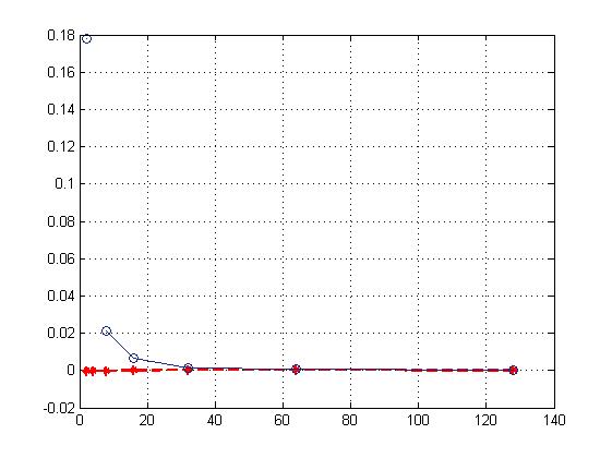
Figure 3. The deviation of the largest Lyapunov exponent from the theoretical prediction. The no-spike case. The dashed line is for Gaussian and the solid line is for Bernoulli matrices. The horizontal axis shows the size of the matrix.
Refer to caption
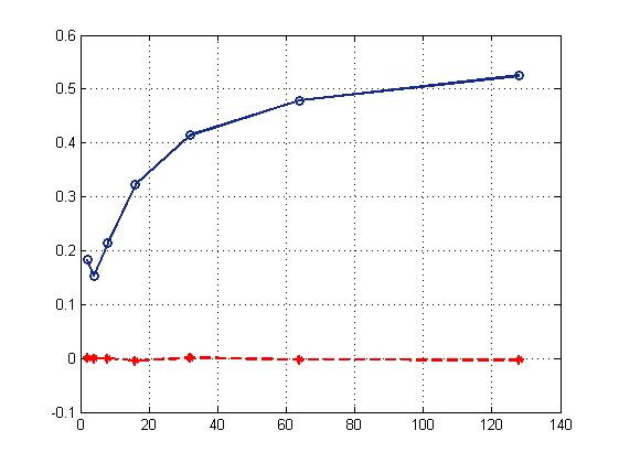
Figure 4. The deviation of the largest Lyapunov exponent from the theoretical prediction. The spike case.

An interesting question is whether the asymptotic expressions derived in this paper remain valid for non-Gaussian random matrices with independent entries. Some numerical evidence concerning this question is presented in Figures 3 and 4.

In order to create plots in these figures, we estimate the Lyapunov exponent using simulations and then plot its difference from the theoretical prediction in the formula (1). The difference is shown against the dimension of the matrix in order to check whether it declines with the increase in dimension as the concept of universality would predict.

Figure 3 presents this plot for the matrices G​A,𝐺𝐴GA, where G𝐺G is the diagonal matrix with half of the diagonal entries equal to 111 and the remaining half equal to 2.22. The dashed line is for a d𝑑d-by-d𝑑d Gaussian matrix A𝐴A where each entry is independent and have variance dβˆ’1.superscript𝑑1d^{-1}. It is very close to zero even for relatively small d.𝑑d.

The solid line is for a d𝑑d-by-d𝑑d matrix A𝐴A where each entry is independent and equals Β±dβˆ’1/2plus-or-minussuperscript𝑑12\pm d^{-1/2} with probability 1/2.121/2. The solid line approaches zero as d𝑑d grows, which suggests that the theoretical approximation gives a good approximation for the Lyapunov exponent of the Bernoulli matrix A.𝐴A.

(This numerical evidence should be taken with a grain of salt. While it might indicate the universality of the theoretical approximation for a large class of matrices, in fact this approximation is not valid for Bernoulli matrices (at least in the strict sense). Indeed, with positive probability the Bernoulli matrix A𝐴A will have all entries equal to dβˆ’1/2superscript𝑑12d^{-1/2} and therefore the starting vector will be mapped to a vector proportional to (1,…,1,2,…,2).1…12…2\left(1,\ldots,1,2,\ldots,2\right). For dβ‰₯4,𝑑4d\geq 4, this vector has a positive probability to be mapped to 00 by an appropriate Bernoulli matrix A.𝐴A. Hence, with probability 111 the product of independent matrices Aksubscriptπ΄π‘˜A_{k} will eventually maps an arbitrary starting vector to zero. It can be seen that this happens for d=4𝑑4d=4 in our plot where the data point is missing. However, for large d𝑑d the simulations would need a prohibitively large time to detect this phenomenon.)

Figure 4 shows an analogous plot for the case when the matrix G𝐺G has a spike. Namely, G𝐺G is assumed to be diagonal with all diagonal entries except one equal to 111 and the exceptional diagonal entry equal to d.𝑑d. This plot shows that the theoretical approximation from Theorem 1.1 is valid for Gaussian but invalid for Bernoulli matrices. This raises a natural question of how the approximation should be modified for large non-Gaussian matrices with a spike in the covariance matrix.


References

  • [1] Patrick Billingsley. Probability and Measure. John Wiley and Sons, third edition, 1995.
  • [2] P.Β Bougerol and J.Β Lacroix. Products of random matrices with applications to Schrodinger operators, volumeΒ 8 of Progress in probability and statistics. Birkhauser: Boston, 1985.
  • [3] JoelΒ E. Cohen, Harry Kesten, and CharlesΒ M. Newman, editors. Random Matrices and Their Applications, volumeΒ 50 of Contemporary Mathematics. American Mathematical Society, 1986.
  • [4] JoelΒ E. Cohen and CharlesΒ M. Newman. The stability of large random matrices and their products. Annals of Probability, 12:283–310, 1984.
  • [5] P.Β J. Forrester. Lyapunov exponents for products of complex Gaussian random matrices. Journal of Statistical Physics, 151:796–808, 2013. arxiv:1206.2001.
  • [6] H.Β Furstenberg and H.Β Kesten. Products of random matrices. Annals of Mathematical Statistics, 31:457–469, 1960.
  • [7] Harry Furstenberg. Noncommuting random products. Transactions of the American Mathematical Society, 108:377–428, 1963.
  • [8] Y.Β Guivarch and A.Β Raugi. Frontiere de Furstenberg, proprietes de contraction et theoremes de convergence. Zeit. Fur Wahrscheinlichkeitstheorie und Verw. Gebiete, 67:265–278, 1985.
  • [9] V.Β Kargin. The norm of products of free random variables. Probability Theory and Related Fields, 139:397–413, 2007. arxiv:math/0611593.
  • [10] V.Β Kargin. Lyapunov exponents of free operators. Journal of Functional Analysis, 255:1874–1888, 2008. arxiv:0712.1378.
  • [11] Emile leΒ Page. RΓ©gularitΓ© de plus grand exposant charactΓ©ristique de produit de matrices alΓ©atoires indΓ©pendantes et applications. Annales de l’Institut Henri Poincar . Probabilit s et Statistiques, 25:109–142, 1989.
  • [12] David Mannion. Products of 2​x​22π‘₯22x2 random matrices. Annals of Applied Probability, 3:1189–1218, 1993.
  • [13] Jens Marklof, Yves Tourigny, and Lech Wolowski. Explicit invariant measures for products of random matrices. Transactions of the American Mathematical Society, 360:3391–3427, 2008.
  • [14] C.Β M. Newman. Lyapunov exponents for some products of random matrices: Exact expressions and asymptotic distributions. In JoelΒ E. Cohen, Harry Kesten, and CharlesΒ M. Newman, editors, Random Matrices and Their Applications, volumeΒ 50 of Contemporary Mathematics, pages 183–195. American Mathematical Society, 1986.
  • [15] CharlesΒ M. Newman. The distribution of Lyapunov exponents: Exact results for random matrices. Communications in Mathematical Physics, 103:121–126, 1986.
  • [16] V.Β I. Oseledec. A multiplicative ergodic theorem. Ljapunov characteristic numbers for dynamical systems. Transactions of the Moscow Mathematical Society, 19:197–231, 1968.
  • [17] Yuval Peres. Domains of analytic continuation for the top Lyapunov exponent. Ann. I. H. Poincare, 28:131–148, 1992.
  • [18] Mark Pollicott. Maximal Lyapunov exponents for random matrix products. Inventiones Mathematicae, 181:209–226, 2010.
  • [19] M.Β S. Raghunathan. A proof of Oseledec’s multiplicative ergodic theorem. Israel Journal of Mathematics, 32:356–362, 1979.
  • [20] David Ruelle. Analyticity properties of the characterisic exponents of random matrix products. The Advances of Mathematics, 32:68–80, 1979.
  • [21] David Ruelle. Characterisic exponents and invariant manifolds in Hilbert space. The Annals of Mathematics, 115:243–290, 1982.
  • [22] David Ruelle. Characterisic exponents for a viscous fluid subjected to time dependent forces. Communications in Mathematical Physics, 93:285–300, 1984.