Driven flow with exclusion and transport in graphene-like structures

Abstract

We study driven flow with exclusion in graphene-like structures. The totally asymmetric simple exclusion process (TASEP), a well-known model in its strictly one-dimensional (chain) version, is generalized to cylinder (nanotube) and ribbon (nanoribbon) geometries. A mean-field theoretical description is given for very narrow ribbons ("necklaces"), and nanotubes. For specific configurations of bond transmissivity rates, and for a variety of boundary conditions, theory predicts equivalent steady state behavior between (sublattices on) these structures and chains. This is verified by numerical simulations, to excellent accuracy, by evaluating steady-state currents. We also numerically treat ribbons of general width. We examine the adequacy of this model to the description of electronic transport in carbon nanotubes and nanoribbons, or specifically-designed quantum dot arrays.

I Introduction

The impact of geometric and topological aspects of the atomic arrangements of materials on its electronic properties has been recognized for quite some time Kittel . A remarkable example is carbon (C), for which different bonding and valence states of C result in stable configurations of C-only based materials in all dimensions D, namely 3D - diamond, graphite, amorphous C, 2D - graphene, 1D - nanotubes (CNT), nanoribbons (CNR), and 0D - fullerenes RMP . Except for diamond, ordered C-based materials of all dimensionalities are constituted of stacked, deformed, or fragmented 2D graphene, which may thus be considered as the basic building block of all forms.

Here we use a simple model to investigate transport properties on the hexagonal geometries of the CNT and CNR structures. These systems are widely accepted as being 1D, based on aspect ratio criteria. For processes such as current flow, e.g. having bias and collective aspects analogous to those from Coulomb blockade, one can question how the geometry affects the behavior and in particular ask whether the physical quantity of interest in the system is indeed equivalent to what is expected from a bona fide 1D system. The honeycomb structure of graphene implies a topology very different from a genuine 1D linear atomic array, where a one-to-one correspondence of bonds and atoms is trivially given; as seen in Sec. II, it requires introducing additional parameters in the model used here.

We do not attempt a realistic description of electronic transport in C allotropes under an applied bias, which requires quantum mechanical description of the electrons in the respective ordered structure potential, as presented, e.g., in Refs. Caio_1, ; Caio, . Instead, we take a complementary viewpoint by generalizing a very simple transport model, extensively studied in 1D lattices, to graphene-like nanotube and nanoribbon structures. This highlights the effect of the topology of the underlying skeleton on transport, allowing direct and unambiguous comparison between such systems and the well-established linear chain results obtained within the same model, namely the totally asymmetric simple exclusion process (TASEP) derr98 ; sch00 ; mukamel ; derr93 ; rbs01 ; be07 ; cmz11 . We find that within certain plausible assumptions nanotubes can be close to exact realizations of 1D systems while, surprisingly, narrow nanoribbons deviate substantially from 1D behavior, which is however obtained only in the limit of very wide ribbons.

The TASEP is among the simplest models in non-equilibrium physics, while at the same time exhibiting many non-trivial properties including flow phase changes, because of its collective character derr98 ; sch00 ; mukamel ; derr93 ; rbs01 ; be07 ; cmz11 . The TASEP and its generalizations have been applied to a broad range of non-equilibrium physical contexts, from the macroscopic level such as highway traffic sz95 to the microscopic, including sequence alignment in computational biology rb02 and current shot noise in quantum-dot chains kvo10 .

In the time evolution of the $1+1$ dimensional TASEP, the particle number $n_{\ell}$ at lattice site $\ell$ can be $0$ or $1$, and the forward hopping of particles is only to an empty adjacent site. In addition to the stochastic character provided by random selection of site occupation update rsss98 ; dqrbs08 , the instantaneous current $J_{\ell,\ell+1}$ across the bond from $\ell$ to $\ell+1$ depends also on the stochastic attempt rate, $p_{\ell}$, associated with it. Thus,

$$J_{\ell,\ell+1}=\begin{cases}{n_{\ell}(1-n_{\ell+1})\quad{\rm with\ probability}\ p_{\ell}}\cr{0\qquad\qquad\qquad{\rm with\ probability}\ 1-p_{\ell}\ .}\end{cases}$$ (1)

In Ref. kvo10, it was argued that the ingredients of TASEP are expected to be physically present in the description of electronic transport on a quantum-dot chain; namely, the directional bias would be provided by an external voltage difference imposed at the ends of the system, and the exclusion effect by on-site Coulomb blockade.

Here we exploit the consequences of applying a similar scenario to graphene-like geometries. In Section II a general mean-field theoretic approach is developed, for the problem of driven flow with exclusion in two-dimensional structures which are cutouts [ "necklaces" (to be defined below), or cylinders, or ribbons etc ] from a honeycomb lattice. Fundamental relationships, like that between the steady-state current $J$ and (i) the (site-averaged) particle density (for periodic boundary conditions [ PBC ]) or (ii) the injection/ejection parameters $\alpha$, $\beta$ (for systems with open ends) are given. Density profiles throughout the system are discussed as well, and these exhibit qualitative differences from the linear chain, especially sublattice character and a loss of particle-hole symmetry.

The most basic structure which, while departing as little as possible from the well-known strictly one-dimensional case, already displays sites with three-fold coordination, is the necklace depicted in Fig. 1. Accounting for the direction of current flow, such sites can act either as "forking" points, or as "bottlenecks". Boundary conditions perpendicular to the flow direction are free. For the case of Fig. 1 one has open boundary conditions at both ends. There, the externally-imposed parameters are: the injection (attempt) rate $\alpha$ at the left end, and the ejection rate $\beta$ at the right one.

Figure 1: Necklace structure for TASEP with open boundary conditions at both ends, and corresponding injection and ejection rates $\alpha$ and $\beta$, respectively. Boundary conditions across direction of flow are free.

Generalizations of the necklace are the cylinder– (nanotube) or ribbon–like structures (see Fig. 2). As seen in that Figure, the nanotube and ribbon geometries considered here correspond, respectively, to zigzag (CNT) and armchair (CNR) configurations of the quasi-1D carbon allotropes RMP . These configurations have no bonds orthogonal to the mean flow direction; thus they fall easily within the generalized TASEP description to be used, where each bond is to have a definite directionality, compatible with that of average flow.

All these structures are amenable to the mean field approach introduced and developed in Sections II.1 and II.2. Sections II.3 and II.4 concern boundary effects and extensions. Some special cases are highlighted in which exact solutions are possible.

Figure 2: Planified section of a nanotube structure with $N_{w}=3$ hexagons round. The dashed lines indicate the "wraparound" bonds which fulfil periodic boundary conditions across the flow direction (for a nanoribbon, such bonds would be absent). For clarity, bond directionalities are omitted, except for wraparound bonds.

Numerical tests of the theory are given in Section III. In Section III.1 we describe the general approach, pointing out details of the calculational method which are expected to reflect properties of the actual transport process in graphene-like samples. Section III.2 provides results for the necklace structure. Section III.3 deals with honeycomb structures of arbitrary width with PBC across the flow direction (nanotubes), and gives numerical results of pertinent simulations. In Section III.4 we consider honeycomb structures (ribbons) with free boundary conditions across the flow direction, and report results of numerical simulations. In Section IV, we summarize our results, and discuss the possible pertinence of the TASEP model results in the context of transport in physical systems such as CNT, CNR, and quantum dot arrays. Concluding remarks are also presented there.

II Theory

II.1 Introduction

The emphasis here and throughout the paper is on steady-state properties of the TASEP on generalized geometries. The microscopic variables, i.e., occupation probabilities $\tau_{i}$ for each site $i$, satisfy a hierarchy of dynamic equations each relating $n-$ and $(n+1)-$body correlations.

In the steady state, the first of these becomes mean current conservation at any site. Even here exact solution (requiring the whole hierarchy) is difficult, but can be achieved in the simplest case of the linear chain with uniform bond rates derr98 ; sch00 ; rbs01 . For this case mean field (factorization of correlations) already gives an extremely useful account of steady-state properties, some of which, like critical current, are exactly provided.

In what follows, the mean field procedure is extended to the new geometries. With uniform bias, equal average site occupations give (in mean field) equal currents on each bond. This gives a steady state for the chain. However, all the geometries considered here have "branchings" at sites with coordination number $z=3$, where typically the division or merging of average current prevents equal site occupation from giving a steady state. There are exceptions, e.g., where non-uniform bond rates compensate. Except when this occurs, the steady states have a sublattice character. The simplest of them have mean site occupations uniform on each of a number of sublattices.

For analytic tractability we shall only consider cases where mean flow direction is parallel to one of the lattice directions, and bond rates are independent of coordinate transverse to the flow direction.

For the chain, no sublattice division occurs but it is well known that in general the mean-field site occupation profile has monotonic variations along the flow direction, increasing for $J<J_{c}$ and decreasing for $J>J_{c}$, where $J_{c}$ is the critical current dividing the two phases the profile characterizes. This result emerges from a Mobius-type profile map with $J$-dependent coefficients which relates, for specified $J$, the mean occupation of a site to that of the previous site mukamel .

In the generalized cases, the sublattice structure emerges directly from the detailed form of the mean-field current conservation equations, in terms of $J$ and all bond rates. Mobius maps for the profiles on each sublattice are given by elimination of sites on other sublattices. By procedures similar to that for the chain, the fixed points of the maps yield the special steady states which are uniform on sublattices, as well as critical currents. Away from the fixed points the maps give the spatially dependent generalizations, characteristic lengths etc. Various special characteristics for the chain are generalized, and the particle-hole exchange symmetry known for the chain typically disappears.

II.2 Mean field approach

We first consider the necklace. The mean field current across a bond with hopping rate $p_{ij}$ going from site $i$ to site $j$ is $p_{ij}\,\langle\tau_{i}\rangle\left(1-\langle\tau_{j}\rangle\right)$, where $\langle\tau_{i}\rangle$, $\langle\tau_{j}\rangle$ are the mean occupations of the two sites. The steady-state conservation equations for mean current $J$ are, for the necklace section shown in Fig. 3:

$$J=p\rho(1-x)=2qx(1-y)=2ry(1-z)=2sz(1-\rho^{\prime})\ .$$ (2)

These each relate site occupations $\rho$, $x$, $r$, $s$, and $\rho^{\prime}$ on successive sublattices.

Figure 3: Bond rates $p$, $q$, $r$, $s$ and sublattice occupations $\rho$, $x$, $y$, $z$, $\rho^{\prime}$ for TASEP on necklace structure; see Eq. (2).

Eliminating site occupations between $\rho$ and $\rho^{\prime}$, i.e. on the sublattices other than that which corresponds to $\rho$, $\rho^{\prime}$, gives the relation for specified $J$:

$$\rho^{\prime}=\frac{a\rho-b}{c\rho-d}\ ,$$ (3)

where

$$a=4pqrs-2J\,\left[pqr+pqs+prs\right]+J^{2}\,pr\hskip 11.38092pt$$

$$b=2qJ\,\left[2rs-J(r+s)\right]\hskip 82.51282pt$$

$$c=4pqrs-2Jps(q+r)\hskip 85.35826pt$$

$$d=2qsJ\,\left[2r-J\,\right]\hskip 112.38829pt$$ (4)

The density profile maps for the other sublattices have the same form but with cyclically interchanged rate variables. The map Eq. (3) is of Mobius form; the corresponding Mobius profile map for the TASEP chain mukamel has $d=0$, $a=c$. This simplification is related to a particle-hole symmetry, which is absent in the general necklace, but is restored where the rates satisfy $a+d=c$ (needing $p=2s$, $r=q$, see below).

Iteration of the map for any sublattice gives that sublattice’s density profile. Alternatively, one can use any one sublattice map, e.g. Eq. (3) with Eq. (4), together with Eq. (2), to give all details (including relationships) of the sublattice density profiles. So, among other things, all profiles are critical at the same $J_{c}$.

Assigning a site label $\ell$, increasing to the right, for each sublattice the map Eq. (3), rewritten as $\rho_{\ell+1}=M(\rho_{\ell})$, gives the density profile $\{\rho_{\ell}\}$ for the "chosen" sublattice. The ansatz (see, for the chain, Refs. mukamel, , rbs01, )

$$\rho_{\ell}=A+B\tanh\theta_{\ell}\ ,\quad{\rm where}\quad\theta_{\ell+1}=\theta_{\ell}+\phi\ ,$$ (5)

is consistent with the map provided $\tanh\phi=cB/(cA-d)$ [ from decomposing $\tanh(\theta_{\ell}+\phi)\,$] and [ to satisfy the remaining relations for all $\theta_{\ell}\,$]

$$B(a+d)=2cAB\ ;\quad A(a+d)=b+c(A^{2}+B^{2})\ .$$ (6)

In terms of $\ell_{0}$ such that $\theta_{\ell}=\phi\ell+\theta_{0}\equiv\phi(\ell-\ell_{0})$, one gets:

$$\rho_{\ell}=A+B\,\tanh\left\{\phi(\ell-\ell_{0})\right\}\ ,$$ (7)

where

$$A=\frac{a+d}{2c}\ ,\quad B=\frac{1}{2c}\sqrt{(a+d)^{2}-4bc}\ ,$$ (8)

$$\tanh\phi=\frac{1}{a-d}\sqrt{(a+d)^{2}-4bc}\ .$$ (9)

$A$, $B$, and $\phi$ are all dependent on $J$, since the coefficients $a$, $b$, $c$, $d$ are. For a given set of bond rates, increasing $J$ can take it through a critical value $J_{c}$ at which the square root vanishes and then becomes imaginary; then

$$\rho_{\ell}=A-|B|\,\tan\left\{|\phi|(\ell-\ell_{0})\right\}\ ,\quad J>J_{c}$$ (10)

while Eq. (7) above applies with real $B$, $\phi$ for $J<J_{c}$. This corresponds to a phase change, similarly to the TASEP chain. There, and in the generalized systems being considered, $|\phi|$ is an inverse characteristic length, which diverges at the (continuous) transition. For the chain, but not in general, $A=1/2$, corresponding to the particle-hole symmetry there, and absent for the generalizations.

As for the chain, the fixed points $\rho^{\ast}=\rho^{>},\,\rho^{<}=A\pm B$ of the controlling maps provide the special constant (sublattice) profiles, for $J<J_{c}$. As $J\to J_{c}$, $\rho^{>}$ and $\rho^{<}$ come together, i.e. $B$ goes to zero, as does the inverse length $|\phi|$, corresponding to criticality.

For the nanotube section with the rates and mean site densities shown in Fig. 4, the steady-state current balance equations analogous to Eq. (2) are:

$$J=p\,x(1-y)=2qy(1-x^{\prime})=p\,x^{\prime}(1-y^{\prime})=\cdots$$ (11)

Figure 4: Bond rates $p$, $q$, and sublattice occupations $x$, $y$, $x^{\prime}$, $y^{\prime}$, $x^{\prime\prime}\dots$ for TASEP on nanotube structure. For clarity, wraparound and a few other bonds have been omitted [ refer to Fig. 2 ]. See Eq. (11).

The greater symmetry implies only two sublattices, and gives a simpler description than for the necklace. The consequent sublattice Mobius map for the $x$-sublattice is:

$$x^{\prime}\ (=x_{\ell+1})\ =\frac{ax-b}{cx-d}=M(x=x_{\ell})\ ,$$ (12)

with

$$a=p(2q-J)\ ;\quad b=d=2qJ\ ;\quad c=2pq\ .$$ (13)

Eqs. (7)–(10) also apply here, with $a$, $b$, $c$, $d$ now given by Eq. (13). The map for the $y$-sublattice is similar, but with $2q$ and $p$ interchanged in the expressions for $a$, $b$, $c$, $d$. This implies that for the special case

$$2q=p\qquad\qquad{\rm(nanotube)}$$ (14)

the two sublattice maps are identical. In this case, for adjacent sites in the full sequence $x$, $y$, $x^{\prime}$, $y^{\prime}$, $x^{\prime\prime}$, $y^{\prime\prime}$, $\cdots$ the map is always the same as for the linear chain TASEP. In this sense, for $2q=p$ sublattices are irrelevant and the mean-feld steady state for the nanotube is equivalent to that on the linear chain; the particle-hole symmetry is also recovered.

There is also a special case for the necklace, with the rates (see Fig. 3)

$$q=r=s=\frac{p}{2}\qquad\qquad{\rm(necklace)}$$ (15)

for which it is easy to check that the sublattice profile maps are the same as the fourth-iterated linear chain map. So, as for the nanotube with $2q=p$ the sublattice density profiles are the same as for the chain, except for spatial and rate rescalings.

Eqs. (7), (8), (9), and (10) apply equally well to general necklace and nanotube, as do their detailed consequences such as critical current. Since $J_{c}$ is where $B$ and $\phi$ of Eqs. (8) and (9) vanish, $J_{c}$ is given by solving the relation

$$(a+d)^{2}=4bc$$ (16)

between the $J$-dependent coefficients, given respectively by Eq. (4) for the necklace, and Eq. (13) for the nanotube.

For the necklace this leads to a quartic equation for $J_{c}$, which factorizes for the special case of Eq. (15), yielding $J_{c}=p/4$ as in the equivalent linear chain. Two additional results are worth recording, for comparison with numerical tests of the theory:

$$p=r=s=2q:\quad J_{c}=\frac{p}{3}\ ;\hskip 42.67912pt$$ (17)

$$p=q=r=s:\quad\frac{J_{c}}{p}=0.40277\dots\ .$$ (18)

For the nanotube the equation for $J_{c}$ is quadratic for general rates, resulting in

$$J_{c}=\mu_{2}^{-2}\,\left[\mu_{0}-\sqrt{\mu_{0}^{2}-\mu_{1}^{2}\mu_{2}^{2}}\,\right]\ ,$$ (19)

where $\mu_{0}=2pq(2q+p)$, $\mu_{1}=2pq$, $\mu_{2}=2q-p$, as long as $\mu_{2}\neq 0$; when $p=2q$ as in Eq. (14), $J_{c}=p/4$; this is the case equivalent to the chain. Among other special cases needed later for comparison with simulations is $p=q$, where

$$J_{c}/p=2[3-\sqrt{8}]\qquad({\rm nanotube},\quad p=q)\ .$$ (20)

The above analysis can also provide the characteristic length $\xi\equiv 1/|\phi|$ (kink width, etc). For $J$ near $J_{c}$, $\xi$ is found to diverge like $|J-J_{c}|^{-1/2}$, in general, as for the linear chain. This can be used in the scaling analysis of finite size corrections for the current etc, but not too close to the critical point where fluctuation effects absent from mean field theory are expected to dominate, changing the above exponent.

II.3 Boundary effects

Boundary effects are strongly affected by the sublattice distinctions required in the generalized geometries. Here the sublattice $\tanh$- or $\tan$- density profiles given, respectively, in Eqs. (7) and (10) are qualitatively similar to the linear chain case. The current conservation equations Eqs. (2), (11) show that here, for example a $\tanh$ solution on one sublattice requires one on the other sublattices, so all sublattices are in the same (low- or maximal-) current phase; also, for $J<J_{c}$ where kinks are present in the chain density profile, the same equations imply that the kinks on different sublattices are in neighboring positions. So for example, in an open geometry, a kink near left, or right, or neither boundary on one sublattice implies the same on the other sublattices, so different sublattices also share the same low- or high-density, or coexistence character.

But the details depend crucially on which sublattices the boundary sites sit on, and in particular whether they are on the same sublattice. The same is true with PBC. In the following, where we examine the influence of boundary conditions along the flow direction, we consider only the case of boundary sites on the same sublattice [ which we take as the "chosen" sublattice in Section II.2, see Eqs. (3) and (12) ]. This applies when an integer number $N$ of basic units (one bond attached to the left of a full hexagon) span the system. Any required generalization could be readily made using the relationships between sublattices provided by the current conservation equations (not done here).

II.3.1 PBC

For PBC of the special type just defined, as in the linear chain, the sublattice steady-state density profiles are flat. We focus on the mean-field "fundamental relation" between $J$ and $\langle\rho\rangle$, where the latter is the (sublattice-averaged) global mean density. This is found by obtaining the two flat density profiles for a chosen sublattice, then using the current conservation equations to obtain the corresponding flat density profiles for the other sublattices, and combining them with the correct weights to find $\langle\rho\rangle$, for the given $J$.

For the nanotube this reduces to

$$\langle\rho\rangle-\frac{1}{2}=\pm B(J)=\pm\frac{1}{2c}\sqrt{(a+d)^{2}-4bc}\ ,$$ (21)

with $a$, $b$, $c$, $d$ given by Eq. (13). Inversion gives the fundamental relation, which is always quadratic sufficiently close to the maximum $J_{c}$. Remarkably, for any $p$, $q$ the maximum occurs at $\langle\rho\rangle=1/2$, same as for the linear chain. For the special case $p=2q$ of Eq. (14) the full nanotube result reduces exactly everywhere to

$$J=\frac{p}{4}-p\left(\langle\rho\rangle-\frac{1}{2}\right)^{2}\ ,$$ (22)

as for the chain.

For the necklace the current-density relation is also quadratic close to $J_{c}$:

$$J_{c}-J\propto\left(\langle\rho\rangle-\rho_{\rm max}\right)^{2}\ .$$ (23)

However, $\rho_{\rm max}\neq 1/2$, except in the special cases with $s=q$ [ including that of Eq. (15) with sublattice equivalence to the linear chain ] where a symmetry argument applies, based on particle - hole duality under flow reversal.

In the special case of Eq. (17),

$$J=J_{c}-p\,\frac{32}{27}\left(\langle\rho\rangle-\frac{17}{36}\right)^{2}+\dots$$ (24)

for $J$ near $J_{c}=p/3$ .

II.3.2 Open BC

We next consider open boundary conditions, again with boundary sites on the same "chosen" sublattice.

In the mean field approach, the injection/ejection processes at the left/right ends, with respective attempt rates $\alpha$ and $\beta$, generalize the current conservation conditions expressed in Eqs. (2) and (11) by the extra equations:

$$J=\alpha\left(1-\rho_{\ell=0}\right)=\beta\rho_{\ell=N}\ .$$ (25)

For given internal bond rates these in principle give the, so far free, variables $J$ and $\ell_{0}$, and hence everything in terms of $\alpha$, $\beta$. At the critical condition, where $B$ and $\phi$ of Eqs. (8) and (9) vanish, the extra equations give the critical point in the $(\alpha,\beta)$ plane as

$$(\alpha_{c},\beta_{c})=\left(\frac{J_{c}}{1-A(J_{c})}\,,\,\frac{J_{c}}{A(J_{c})}\right)\ ,$$ (26)

generally without the symmetry of the critical point $(\alpha_{c},\beta_{c})=(p/2,p/2)$ for the chain, where $A=1/2$, $J_{c}=p/4$. E.g., for the nanotube:

$$(\alpha_{c},\beta_{c})=\left(\frac{2\mu_{1}\,J_{c}}{\mu_{1}-\mu_{2}\,J_{c}}\,,\,\frac{2\mu_{1}\,J_{c}}{\mu_{1}+\mu_{2}\,J_{c}}\right)\ ,$$ (27)

in terms of the variables defined in connection with Eq. (19), while for the necklace with $p=r=s=2q$,

$$(\alpha_{c},\beta_{c})=\left(p,\frac{p}{2}\right)\ .$$ (28)

By considering sublattice kinks near the system’s boundaries, it can be shown that in mean-field theory the phase boundaries are vertical and horizontal lines in the $\alpha-\beta$ plane through and outwards from the critical point.

With $(\alpha,\beta)$ sufficiently below $(\alpha_{c},\beta_{c})$ the equations are consistent with $J<J_{c}$ and kink width $\phi^{-1}$ not very large. Then the constraint equations, Eq. (25), can be consistent with having the sublattice kinks away from the boundaries, so that the relations of $\alpha$, $\beta$ to profile values $A\pm B$ are:

$$\alpha\,\left[1-\left(A(J)-B(J)\right)\right]=\beta\,\left[A(J)+B(J)\right]=J<J_{c}\ .$$ (29)

For given rates this is a parametric equation in $J$ for a curve (the coexistence line) in the $\alpha-\beta$ plane. For the nanotube this becomes

$$2pq(\alpha-\beta)=(2q-p)\alpha\beta\ .$$ (30)

For both necklace and nanotube it can be easily established that the coexistence line joins the origin to the critical point, and though it is in general not straight its slope at the origin is always unity.

II.4 Extensions

In the preceding mean-field discussion, the simplest situation has been where profiles are flat on sublattices. For the chain this is known to be an exact property under special conditions where correlation functions factorize; then size dependences disappear derr93 . Here we consider this possibility for necklaces and nanotubes with open boundary conditions.

We start by assuming factorization in the sense that occupations $\tau_{i}$ are the same on all sites of a sublattice but different between sublattices. This is consistent with exact average-current conservation (the first member of the hierarchy of exact steady state correlation function equations). Since no occupation variable occurs squared in those equations, it is also consistent with our generalized mean field approximation, including the Mobius maps and their consequences as spelt out in Section II.2, but only under conditions where those give a constant profile on each sublattice, i.e., fixed points $\rho^{\ast}$. Adding the injection/ejection constraints, Eq. (25), the flat fixed point profiles will not in general be consistent with the latter, unless

$$\alpha\,\left[1-\rho^{\ast}(J)\right]=J=\beta\,\rho^{\ast}(J)\ .$$ (31)

So a necessary condition for the factorization to give an exact solution is that ($\alpha$, $\beta$) lies on the line in the $(\alpha,\beta)$ plane whose parametric equation is Eq. (31). The remaining condition for sufficiency is that factorization is consistent with all the other members of the hierarchy of internal correlation function equations (not proven here).

For the general nanotube, elimination of $J$ from Eq. (31) gives the "factorization line" as

$$\frac{\alpha}{2q}+\frac{\beta}{p}=1\ .$$ (32)

This line goes through the critical point $(\alpha_{c},\beta_{c})$ of Eq. (27), and becomes the same as for the chain if $2q=p$ [ see Eq. (14) ].

Quadratic $J$-dependences in the map coefficients for the necklace complicate the analysis, but the line (now curved) again goes through $(\alpha_{c},\beta_{c})$ of Eq. (27); the special case $q=r=s=p/2$ again becomes that for the chain [ see Eq. (15) ].

In Section III we provide numerical checks of selected predictions of the mean-field theory just described, namely steady-state currents and their dependence on average particle density (for PBC) or on injection/ejection attempt rates (for systems with open boundaries), for both necklaces (Section III.2) and nanotubes (Section III.3), all for assorted bond rate combinations of interest. For nanoribbons the translational symmetry perpendicular to flow direction (crucial in the reduction of the number of sublattices for the nanotube, see Eq. (11) and Fig. 4) is lost with free boundary conditions at the edges. Thus, in this case we restricted ourselves to the numerical simulations described in Sec. III.4 .

Finally, we performed some numerical tests of factorization for nanotubes with open boundary conditions [ see Eqs. (31) and (32) above ]. They are briefly reported at the end of Sec. IV.

III Numerics

III.1 Introduction

For simplicity we consider structures with an integer number $N_{r}$ of elementary cells (one bond attached to the left of a full hexagon) along the mean flow direction.

Adapting the procedures used for the $(1+1)-$ dimensional TASEP, an elementary time step consists of $N_{b}$ sequential bond update attempts, each of these according to the following rules: (1) select a bond at random, say, bond $\ell$; (2) if the chosen bond has an occupied site to its left and an empty site to its right, then (3) move the particle across it with probability (bond rate) $p_{\ell}$. If the injection or ejection bond is chosen, step (2) is suitably modified to account for the particle reservoir (the corresponding bond rate being, respectively, $\alpha$ or $\beta$).

One can equally well update sites instead (via $N_{s}$ random sequential site choices). Once a site is picked, (i) if the site is a "forking" one, either of the two bonds to its right is randomly selected [ with probability $1/2$, i.e., no transverse bias is allowed ], and then steps (2) and (3) above are followed; (ii) for open boundary conditions, if the site is the injection (ejection) one, then if it is unoccupied (occupied), a particle is injected into (ejected out of) it with probability $\alpha$ ($\beta$); (iii) otherwise, steps (2) and (3) above are followed right away.

It is easily seen that on average a total of $N_{b}$ update attempts will take place, in the course of a unit time step as defined above, for either bond or site update. In the strictly one-dimensional TASEP, bond- and site update are entirely equivalent. However, for full equivalence between the two methods in the present case, it must be noted that randomly selecting (with $1/2$ probability) which bond to probe, when starting from a "forking" site, effectively halves the following bonds’s rates. For all geometries investigated here we ran simulations using both bond and site update. In all cases for which the effective bond rates (i.e. taking into account the effect just described for site update) coincided, the results given by both methods were indistinguishable within error bars.

Both site and bond update may be relevant in physical applications. We defer a discussion of the potential relationship of each update method to specific features of graphene-like structures to Sec. IV.

Here we evaluate the steady-state current $J$ as the time- and ensemble-averaged number of particles (per unit time) which (a) enter the system [ for open ends ], or (b) cross any single bond connecting adjacent hexagons [ for PBC$\,]$. For systems with $N_{e}>1$ "entry" bonds, such as the nanotubes and ribbons considered, respectively, in Sections III.3 and III.4, one has to divide further by $N_{e}$, to provide proper comparison with the strictly one-dimensional case. Starting from a spatially random configuration of occupied and empty sites, we usually waited $n_{\rm in}=10,000$ time steps for steady-state flow to be fully established, to ensure that our measurements were free from startup effects. After that, we collected steady-state current samples (typically for $N_{\rm sam}=10^{\,6}$ consecutive unit time steps). The accuracy of results was estimated by evaluating the root-mean-square (RMS) deviation among $N_{\rm set}$ independent sets of $N_{\rm sam}$ steady-state samples each. As is well known rbsdq12 , such RMS deviations are essentially independent of $N_{\rm set}$ as long as $N_{\rm set}$ is not too small, and vary as $N_{\rm sam}^{-1/2}$. We generally took $N_{\rm set}=10$.

III.2 The Necklace Structure

The structures considered here have $N_{s}^{P}=6N_{r}$ sites and $N_{b}^{P}=7N_{r}$ bonds (for PBC), or $N_{s}^{O}=6N_{r}+1$ sites [ recall the extra site on the right, connecting to the ejection bond, see Fig. 1 ] and $N_{b}^{O}=7N_{r}+2$ bonds (counting the injection and ejection bonds, for open boundary conditions.

We first check the mean-field prediction, see Eq. (15), that the steady-state current on a system where all bond rates on the hexagons are $1/2$, and those on bonds between hexagons are unity, is the same as on a strictly one-dimensional arrangement. Using site updating procedures, we fixed the nominal bond rates for links on a hexagon immediately following a "forking" site to be unitary, so they would effectively be halved. We also ran simulations using bond update, in which case all hexagon bonds were set to $p=1/2$ from the start, with the same results (within error bars) as those from site update.

For systems with PBC, the current on a strictly one-dimensional lattice with $N$ sites and $M$ particles (average density $\rho=M/N$), and unit bond rates, is mukamel

$$J=\rho\,(1-\rho)\,\frac{N}{N-1}\quad\ (d=1,\ {\rm PBC})\ .$$ (33)

Table 1 illustrates the excellent agreement found between theoretical predictions and numerical simulations for PBC. Remarkably, the identification between necklace- and chain current goes as far as finite-size effects: systems of either type with the same number of sites obey Eq. (33) equally. This is consistent with exact factorizability needing no conditions like Eq. (31) in the case of PBC.

Table 1: For systems with PBC, $N_{s}$ sites, and $\langle\rho\rangle$ as specified, $J_{\rm num}$ is current through necklace (with $N_{r}=N_{s}/6$ rings, effective bond rates $p=1/2$ on hexagons, $p=1$ on bonds between hexagons), as given by numerical simulations with $N_{\rm sam}=10^{\,6}$, $N_{\rm set}=10$ (see text); $J_{\rm 1d}$ is current through one-dimensional system with $N=N_{s}$ , given by Eq. (33) .

$\ \ N_{s}$	$J_{\rm num}$	$J_{\rm 1d}$
$\langle\rho\rangle=1/2$
$\ \ 24$	$0.26081(13)$	$0.260867\dots$
$\ \ 36$	$0.25713(18)$	$0.257143\dots$
$\ \ 48$	$0.25533(11)$	$0.255319\dots$
$\ \ 60$	$0.25426(11)$	$0.254237\dots$
$\ \ 72$	$0.25353(14)$	$0.253521\dots$
$\ \ 84$	$0.25297(10)$	$0.253012\dots$
$\ \ 96$	$0.25261(7)\ \,$	$0.252632\dots$
$\langle\rho\rangle=1/4$
$\ \ 24$	$0.19563(15)$	$0.195652\dots$
$\ \ 36$	$0.19280(7)\ \,$	$0.192857\dots$
$\ \ 48$	$0.19149(11)$	$0.191489\dots$
$\ \ 60$	$0.19066(9)\ \,$	$0.190678\dots$
$\ \ 72$	$0.19015(9)\ \,$	$0.190141\dots$
$\ \ 84$	$0.18971(5)\ \,$	$0.189759\dots$
$\ \ 96$	$0.18945(12)$	$0.189474\dots$

Next we give results for systems with open boundary conditions, also for the special rates of Eq. (15), at selected locations on the $\alpha$–$\beta$ phase diagram; see Table 2. Agreement with mean-field theory (including finite-size effects, or their absence) is very good at $(\alpha,\beta)=(1/2,1/2)$, as well as at $(1/4,1/4)$ [ the latter point corresponding to the coexistence line between high-and low-density phases in the one-dimensional TASEP ]. For $(\alpha,\beta)=(1,1)$, deep within the maximal-current phase of the one-dimensional problem, small discrepancies are present for small systems; however, they tend to vanish as $N_{s}$ increases.

Table 2: For systems with open boundary conditions, $N_{s}$ sites, and $(\alpha,\beta)$ as specified, $J_{\rm num}$ is current through necklace (with $N_{r}=(N_{s}-1)/6$ rings, effective bond rates $p=1/2$ on hexagons, $p=1$ on bonds between hexagons), as given by numerical simulations with $N_{\rm sam}=10^{\,6}$, $N_{\rm set}=10$ (see text); $J_{\rm 1d}$ is current through one-dimensional system, see e.g. Refs. derr93, ; rbsdq12,  .

$\ \ N_{s}$	$J_{\rm num}$	$J_{\rm 1d}$
$(\alpha,\beta)=(1/2,1/2)$
$\ \ 13$	$0.24993(26)$	$1/4$
$\ \ 31$	$0.24996(15)$	$1/4$
$\ \ 61$	$0.24998(10)$	$1/4$
$\ \ 301$	$0.24999(9)\ \,$	$1/4$
$(\alpha,\beta)=(1/4,1/4)$
$\ \ 13$	$0.17479(24)$	$0.175399\dots$
$\ \ 31$	$0.18175(25)$	$0.181903\dots$
$\ \ 61$	$0.18448(27)$	$0.184547\dots$
$\ \ 301$	$0.18688(25)$	$0.186882\dots$
$(\alpha,\beta)=(1,1)$
$\ \ 13$	$0.28303(18)$	$0.277777\dots$
$\ \ 31$	$0.26324(13)$	$0.261905\dots$
$\ \ 61$	$0.25543(7)\ \,$	$0.256098\dots$
$\ \ 301$	$0.25125(10)$	$0.251244\dots$

We now turn to combinations of bond rates for which mean-field solutions are less simple, but which are plausible in terms of potentially describing electronic transport on a graphene-like structure. Assuming the simplest case of lattice homogeneity, we consider uniform rates $p=1$ for all bonds. Except where otherwise noted, we use site update procedures in the simulations described here; thus, as explained above, the bonds immediately following a "forking" site have their effective rates halved.

For the necklace with PBC we calculated steady-state currents for $\langle\rho\rangle=m/12$, $m=1,2,\cdots 11$. For each density we considered rings with $N_{r}=4,6,\cdots,16$ elementary cells. The respective sequences behave smoothly against $N_{r}^{-1}$, and were extrapolated to $N_{r}^{-1}\to 0$ by fits to quadratic polynomials. Final results are shown in Fig. 5. As predicted in Sec. II.3.1, for this case in which $q\neq s$ the particle-hole symmetry is lost. The maximum of the adjusted curve is at $(\langle\rho\rangle,J)=(0.475(3),0.3234(2))$ . The parabolic shape near the maximum, predicted in Eq. (24), is verified, and the numerical value given there for $p=1$, namely $\rho_{c}=17/36=0.4722\dots$, is within error bars; however, the predicted $J_{c}=1/3$ appears to overshoot the numerical result by some $3\%$.

The values of $\rho_{c}$, $J_{c}$ given above are to be compared also with the maximal current for the one-dimensional TASEP with PBC and unit bond rates, namely $J=1/4$ at $\rho=1/2$, see Eq. (33) .

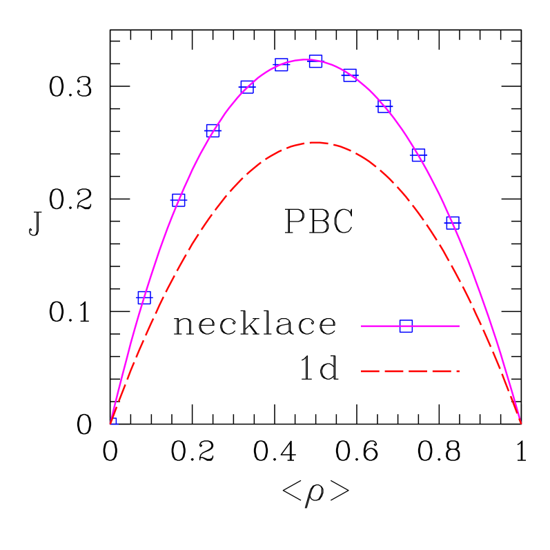
Figure 5: (Color online) Current-density relationship for necklace structure with PBC, all nominal bond rates $p=1$, site update. Points correspond to simulations; the solid curve is a fourth-degree polynomial fit to the data. The long-dashed curve is for the one-dimensional TASEP with PBC.

For the necklace with open boundary conditions, and nominal rates $p=1$ for all internal bonds [ i.e. except for the injection and ejection bonds at the extremes, with their characteristic rates $\alpha$ and $\beta\,$], we first report results on the $\alpha+\beta=1$ line. System sizes were the same as for PBC. The current $J$, parametrized by $\alpha$, is shown in Fig. 6. For the one-dimensional TASEP, the steady-state current is $J=\alpha\beta$ on this line, and is size-independent derr93 . Here we found little size dependence for both $\alpha\lesssim 0.4$ and $\alpha\gtrsim 0.7$. Around the peak shown in Fig. 6, the current distinctly increases with system size, thus we resorted to linear or quadratic fits against $N_{r}^{-1}$ to produce extrapolated values. Comparison with the one-dimensional TASEP would suggest that an increase in $J$ with system size indicates proximity to a coexistence line between low- and high-density phases, see the entries for $(\alpha,\beta)=(1/4,1/4)$ in Table 2. In contrast to the case of PBC, we could not produce a single, smooth fitting function for the $J$ vs. $\alpha$ relationship over the full range $0<\alpha<1$, mainly because of the sharply asymmetric peak. We estimate the largest current along $\alpha+\beta=1$ to be $J=0.3058(2)$ at $\alpha=0.575(3)$.

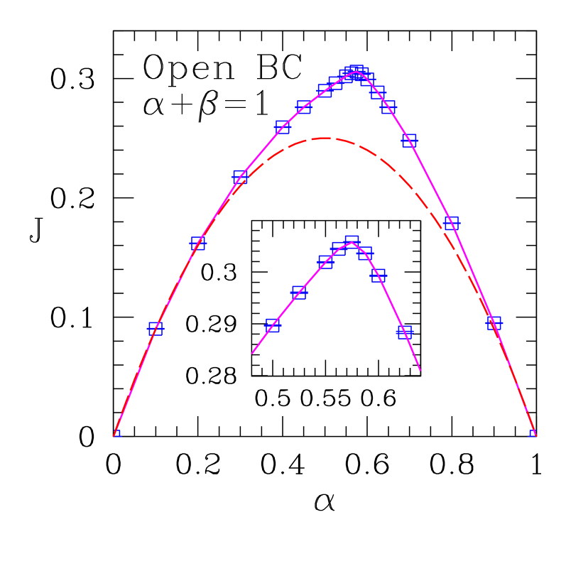
Figure 6: (Color online) Current against injection rate $\alpha$ for necklace structure with open boundaries, along $\alpha+\beta=1$, all nominal bond rates $p=1$, site update. Points correspond to simulations. The long-dashed curve is for the one-dimensional TASEP on the line $\alpha+\beta=1$. Inset: close-up view of peak region. Same axis labels as main figure.

Relying once more on analogies with the one-dimensional TASEP, we examined the region close to $(\alpha,\beta)=(1,1)$ in order to probe the extent of a hypothetical maximal-current phase. Fig. 7 shows the extrapolated ($N_{r}\to\infty$) currents along $\alpha=\beta$, for $0.65\leq\alpha\leq 1$. System sizes used were the same as for PBC, except that for $\alpha>0.7$ we went up to $N_{r}=50$. In the latter region, improved accuracy was necessary in order to distinguish between very similar values (see especially the inset of Fig. 7).

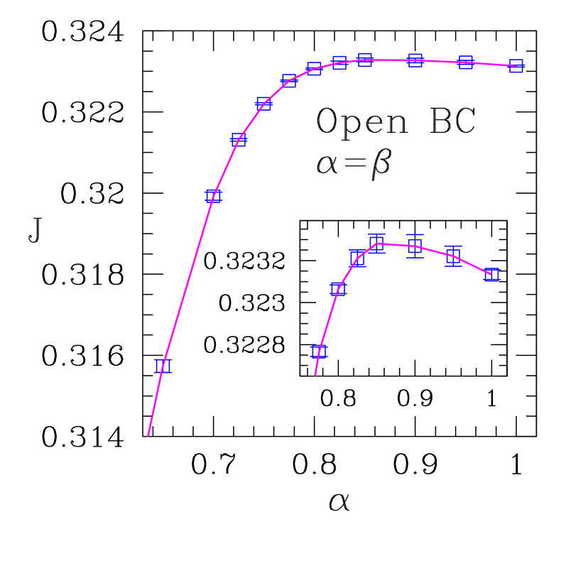
Figure 7: (Color online) Current against injection rate $\alpha$ for necklace structure with open boundaries, along $\alpha=\beta$, all nominal bond rates $p=1$, site update. Points correspond to simulations. Inset: close-up view of region close to $\alpha=1$. Same axis labels as main figure.

Taking account of the error bars for individual results, our tentative conclusion is that the current indeed stabilizes at $J_{\rm max}=0.3232(1)$, and that the section of the $\alpha=\beta$ line for $\alpha\gtrsim 0.825$ is within the maximal-current phase.

The estimate just found for the maximal current is consistent within error bars with the corresponding one for PBC, also with site update and same bond rates, namely $0.3234(2)$. This is to be expected, since regardless of boundary conditions $J_{c}$ is achieved with density profiles $\rho_{c}=\rho^{>}=\rho^{<}$; for open boundary conditions this imposes additional constraints on $\alpha$, $\beta$ [ see Eq. (31) ] while PBC are automatically consistent with flat profiles.

We also checked the prediction of Eq. (18) for the critical current on the necklace with all effective rates equal to unity, by using bond update procedures. For PBC with this particular set of rates, mean field theory predicts (see Sec. II.3.1) that the $J-\langle\rho\rangle$ curve is symmetric about $\langle\rho\rangle=1/2$, thus restoring particle-hole symmetry. A scan through various average densities, similar to that shown in Fig. 5, indeed resulted in a symmetric curve; however, we found $J_{c}=0.3958(4)$, just under $2\%$ below the mean field prediction. With open boundary conditions we scanned the region of the $(\alpha,\beta)$ plane close to $(\alpha,\beta)=(1,1)$ and found a picture qualitatively similar to the one exhibited in Fig. 7. From that we estimate $J_{c}=0.395(1)$, in good agreement with the PBC result.

III.3 Nanotubes

We consider strips of a two-dimensional honeycomb lattice with the same orientation, relative to particle flow direction, as the necklace, and with periodic boundary conditions across the flow direction (recall Figs. 2 and 4). Such "nanotubes" can be seen as $N_{w}$ parallel necklaces, with adjacent necklaces sharing edges parallel to the flow direction, as well as the corresponding sites. The total number of sites is thus $N_{s}^{P}=N_{w}\times 4N_{r}$ for PBC, or $N_{s}^{O}=N_{w}\times(4N_{r}+1)$ for open boundary conditions at the ends. As remarked in Sec. III.2, the normalized current $J$ in this case is the (average) total number of particles moving through a fixed cross-section of the system, per unit time, divided by $N_{w}$.

According to Eqs. (14) and (22), for the case where all bonds parallel to the flow direction have rates $p$, and all others have $p/2$, the current is the same as on a one-dimensional lattice with all bond rates equal to $p$. For the nanotube, such (effective) rates correspond to the physically plausible assumption of equal nominal rates $p=1$ on all bonds, together with the use of site update procedures.

We first examine a toroidal geometry, i.e., one with PBC in both directions. The finite-length effects on the one-dimensional lattice, which come via the $N$-dependent factor in Eq. (33), here correspond to the total number of sites on the nanotube, i.e. $N=N_{w}\times 4N_{r}$, independent of the aspect ratio $A\equiv N_{w}/4N_{r}$. This is illustrated by the results in Table 3.

Table 3: For systems with $N_{s}$ sites, and $\langle\rho\rangle=1/2$, $J_{\rm num}$ is current through toroid of width $N_{w}$, length $N_{r}$ rings ($N_{s}=N_{w}\times 4N_{r}$), effective bond rates $p=1$ on bonds parallel to flow direction,, $p=1/2$ otherwise, as given by numerical simulations with $N_{\rm sam}=10^{\,6}$, $N_{\rm set}=10$ (see text); $J_{\rm 1d}$ is current through one-dimensional system, given by Eq. (33) .

$\ \ N_{s}$	$N_{w}$	$N_{r}$	$J_{\rm num}$	$J_{\rm 1d}$
$\ \ 80$	$4$	$5$	$0.253172(74)$	$0.2531646\dots$
$\ \ 96$	$2$	$12$	$0.252635(51)$	$0.2526316\dots$
$\ \ 96$	$3$	$8$	$0.252641(57)$	$0.2526316\dots$
$\ \ 96$	$4$	$6$	$0.252656(45)$	$0.2526316\dots$
$\ \ 96$	$6$	$4$	$0.252626(49)$	$0.2526316\dots$
$\ \ 96$	$8$	$3$	$0.252645(61)$	$0.2526316\dots$
$\ \ 96$	$12$	$2$	$0.252636(46)$	$0.2526316\dots$
$\ \ 160$	$4$	$10$	$0.251589(39)$	$0.2515723\dots$

We checked the predictions associated with Eq. (14) for a nanotube with open boundary conditions at the ends, at selected locations on the $\alpha$–$\beta$ phase diagram; see Table 4. Agreement with mean-field theory is very good at $(\alpha,\beta)=(1/2,1/2)$; at $(1/4,1/4)$ and, especially, at $(\alpha,\beta)=(1,1)$, differences between finite-lattice numerical results for the nanotube and the corresponding exact ones for the chain are somewhat significant (up to $5\%$ for $N_{s}=104$ at the latter point) for small systems; however, they tend to vanish as $N_{s}$ increases.

Table 4: For systems with open boundary conditions, $N_{s}$ sites, and $(\alpha,\beta)$ as specified, $J_{\rm num}$ is current through nanotube of width $N_{w}$, length $N_{r}$ rings ($N_{s}=N_{w}\times(4N_{r}+1)$), effective bond rates $p=1$ on bonds parallel to flow direction,, $p=1/2$ otherwise, as given by numerical simulations with $N_{\rm sam}=10^{\,6}$, $N_{\rm set}=10$ (see text); $J_{\rm 1d}$ is current through one-dimensional system, see e.g. Refs. derr93, ; rbsdq12,  .

$\ \ N_{s}$	$N_{w}$	$N_{r}$	$J_{\rm num}$	$J_{\rm 1d}$
$(\alpha,\beta)=(1/2,1/2)$
$\ \ 104$	$8$	$3$	$0.249994(65)$	$1/4$
$\ \ 200$	$8$	$6$	$0.250006(44)$	$1/4$
$\ \ 246$	$6$	$10$	$0.250011(36)$	$1/4$
$\ \ 390$	$6$	$16$	$0.249992(31)$	$1/4$
$(\alpha,\beta)=(1/4,1/4)$
$\ \ 104$	$8$	$3$	$\!\!0.18390(7)$	$0.18575\dots$
$\ \ 200$	$8$	$6$	$0.18620(11)$	$0.186574\dots$
$\ \ 246$	$6$	$10$	$0.18661(11)$	$0.186745\dots$
$\ \ 390$	$6$	$16$	$\!\!0.18694(9)$	$0.187022\dots$
$(\alpha,\beta)=(1,1)$
$\ \ 104$	$8$	$3$	$0.267521(56)$	$0.2535888\dots$
$\ \ 200$	$8$	$6$	$0.256993(40)$	$0.2518703\dots$
$\ \ 246$	$6$	$10$	$0.253495(34)$	$0.2515213\dots$
$\ \ 390$	$6$	$16$	$0.251827(34)$	$0.2509603\dots$

We also probed the case with all effective bond rates $p=q=1$. Finite-size effects were generally dealt with by considering systems of varying widths ($N_{w}\lesssim 15$ rings), and lengths ($N_{r}\lesssim 50$ rings). Within these ranges we found that results became essentially independent of $N_{w}$; for fixed (large) $N_{w}$ we extrapolated the corresponding sequences of finite-length currents against $N_{r}^{-1}$ via linear, or at most quadratic, fits. With PBC, we confirmed that the maximal current is found at $\langle\rho\rangle=1/2$, consistent with theory (see Sec. II.3.1). However, numerics gives $J_{c}=0.3492(1)$, slightly above the prediction of Eq. (20). With open boundary conditions at the ends, evaluating currents at and near $(\alpha,\beta)=(1,1)$ again gives $J=0.3492(1)$, agreeing with the PBC result to four significant digits.

III.4 Ribbons

Here, we only consider open boundary conditions at the ribbon’s ends, and all nominal bond rates are taken as unitary. Initially we use site update procedures, which halves the effective rates for nearly all bonds not parallel to the mean flow direction. The difference to the nanotubes of Sec. III.3 [ where all such bonds have their rates halved, thus the system’s rates are given by Eq. (14) ] is a boundary effect: it arises because those bonds on the ribbons’ edges, along which the flow goes inward, do not immediately follow a "forking" site, see Fig. 2. The effective rates of such bonds then remain equal to their nominal value. Therefore, one expects the discrepancies between steady-state currents on ribbons and on nanotubes to vanish as the number $N_{w}$ of elementary units across both systems increases. It was predicted in Sec. II.2, and numerically verified in Sec. III.3, that nanotubes with effective bond rates given by Eq. (14) behave effectively as one-dimensional systems, so this must also be the asymptotic behavior of ribbons. We have checked, for selected points on the $(\alpha,\beta)$ phase diagram, that this indeed happens, only with finite-width (and -length) effects generally more significant than for nanotubes; see Fig. 8.

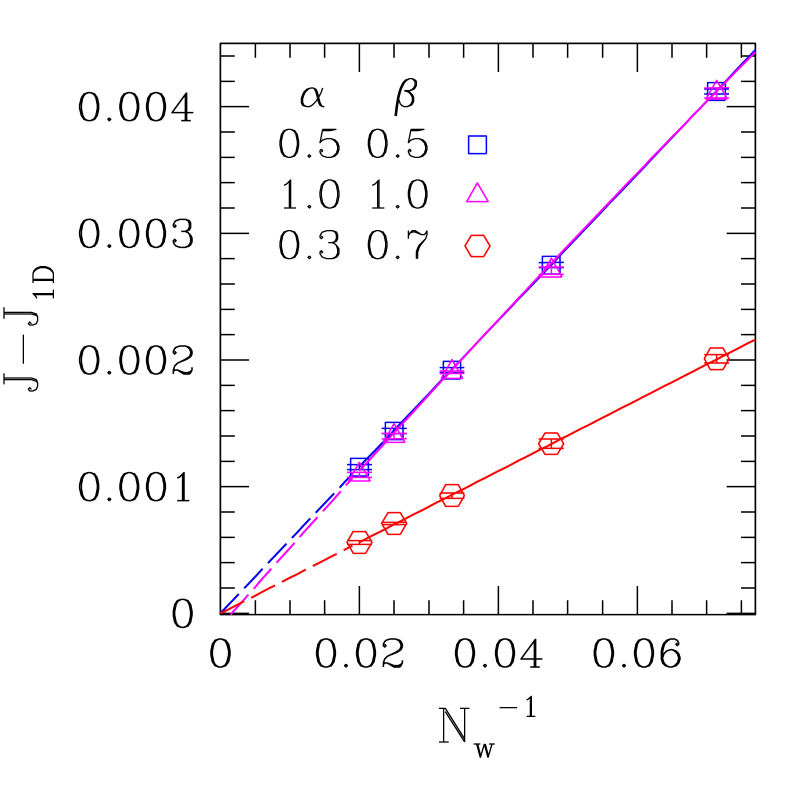
Figure 8: (Color online) Simulation results for current against inverse system width $N_{w}^{-1}$ for nanoribbons with open boundary conditions, all nominal bond rates equal to unity, site update. Each point represents previous extrapolation to $N_{r}\to\infty$ at fixed $N_{w}$. $J_{1D}$ is the $N_{r}\to\infty$ current for one-dimensional systems with the same injection and ejection rates: $J_{1D}=0.25$ for $(\alpha,\beta)=(0.5,0.5)$ and $(1.0,1.0)$, and $0.21$ for $(\alpha,\beta)=(0.3,0.7)$. The lines are quadratic fits to data.

We also made all effective rates equal to unity, by using bond update procedures. We concentrated on evaluating the maximal (or critical) current across the system, by making $\alpha=\beta=1$. For fixed width $N_{w}$, we produced sequences of steady-state current estimates with growing length $N_{r}\leq 50$. By fitting such sequences to parabolic forms in $N_{r}^{-1}$, we found that the extrapolated values [ for $N_{r}\to\infty\,$] $J_{\infty}(N_{w})$ still depended significantly on $N_{w}$. Finally, we extrapolated the sequence of $J_{\infty}(N_{w})$ against $N_{w}^{-1}$, finding $J_{c}=\lim_{N_{w}\to\infty}J_{\infty}(N_{w})=0.3493(1)$.

IV Discussion and Conclusions

We have presented a mean-field theory for driven flow with exclusion in graphene-like structures, and numerically checked its predictions for steady state current on the necklace and nanotube structures, with both PBC and open boundary conditions at the ends.

For all bond rate combinations in which the mean field mapping reduces to the chain case, currents on necklaces and nanotubes match those in the strictly one-dimensional systems. For PBC this includes finite-size effects, see Tables 1 and 3. For open boundary conditions, the absence of size dependence on the factorizable line $\alpha+\beta=1$ is reproduced; away from that line, finite-system corrections slightly differ from 1D ones, but discrepancies die away as system size increases (see Tables 2 and 4).

With bond rates such that no reduction to the chain case occurs, the maximal (critical) currents $J_{c}^{\,\rm MF}$ predicted by mean field theory [ see Eqs. (17),  (18), (20) ], appear to be slightly off numerical results, $J_{c}^{\,\rm num}$ (at most by $2-3\%$). Interestingly, for the cases just mentioned, one has $J_{c}^{\,\rm MF}>J_{c}^{\,\rm num}$ for the necklace, while $J_{c}^{\,\rm MF}<J_{c}^{\,\rm num}$ for the nanotube.

Symmetry, or lack thereof, of the fundamental current-density relationship for PBC and general bond rates is correctly predicted by mean field theory (necklace and nanotube), see Sec. II.3.1.

In this and the following paragraph, we only refer to the special case with all nominal bond rates equal to unity. We found in Sec. III.2 that the maximal (critical) current on the necklace structure is $J_{c}=0.3233(3)$ for site update, and $J_{c}=0.395(1)$ for bond update, to quote an aggregate of the results given there. For nanotubes, the mean-field theory of Sec. II.2 predicts equivalence to the one-dimensional TASEP for the bond rates quoted in Eq. (14). Such rates are effectively reproduced by using site update with all nominal bond rates unitary. So, if the actual transport mechanism on zigzag CNTs displays the characteristics of site update, one would expect such structures to behave as effectively (rather than quasi-) one-dimensional.

For nanoribbons, no mean-field theory has been developed here, for reasons explained at the end of Sec. II.4. However, the considerations of Sec. III.4 show that broad ribbons should carry the same current as nanotubes (although finite-size effects can be rather significant), so e.g. for site update and $N_{w}\gg 1$ the maximal current on both structures approaches $J_{c}=1/4$. This is verified numerically, as illustrated in Fig. 8. For bond update, our data are summarized in Fig. 9, which pertains both to Sec. III.3 and to Sec. III.4. Fig. 9 strongly suggests that both types of structure asymptotically support the same maximal current also when all effective rates are equal. We quote $J_{c}=0.3492(2)$, allowing for the uncertainties of all three sequences of estimates displayed there.

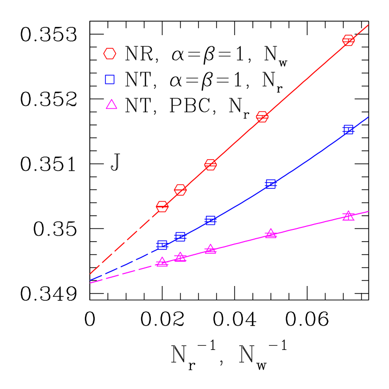
Figure 9: (Color online) For all effective bond rates equal to unity, current against inverse system size $N_{r}^{-1}$ (triangles, squares) or $N_{w}^{-1}$ (hexagons; each point represents previous extrapolation to $N_{r}\to\infty$ at fixed $N_{w}$). Hexagons: nanoribbons (NR) with open boundary conditions, $\alpha=\beta=1$. Squares: nanotubes (NT) with open boundary conditions, $\alpha=\beta=1$. Triangles: NT with PBC, $\langle\rho\rangle=1/2$ (corresponding to maximal current, see Sec. II.3.1). Points correspond to simulations.

Regarding the applicability of the generalized TASEP model discussed here to experimentally realized systems, we first note that transport in CNT and CNR is predominantly governed by band electrons RMP , for which neither a bond nor a site can be uniquely assigned at any time-step. Nevertheless, residual signatures of the topology of the hexagonal skeleton can be expected to remain, such as the trend followed by (normalized) current against increasing width, seen in Figs. 8 and 9. On the other hand, finer details of the TASEP behavior unveiled here possibly have no discernible counterparts in such C-based materials.

Turning now to quantum dot (QD) systems, site update would be adequate, e.g., to model QD arrays in which the electron remains bound to a specific QD for dwell times much longer than the inverse hopping attempt rate onto a neighboring QD.

One might consider, e.g., a honeycomb arrangement of QDs, so that each QD may be empty or occupied by one electron, while a second electron is excluded by Coulomb blockade. Electrostatically defined QD arrays have already been fabricated via electrodes over a two-dimensional electron gas on a semiconductor/barrier interface IvW11 . Recent experimental investigations of electron hopping transport in systems of self-assembled QD chains indicate that such studies in more complex geometries may soon be accessible jap13 .

Of course planar arrangements of QDs provide a physical realization of a nanoribbon, but not a nanotube. For a QD array forming a ribbon-shaped cutout (along a given bond direction) of the honeycomb lattice, individual tunnel barrier strengths could be tuned by the electrodes shaping the confining potential, thus defining the bond rates. The various bond rates considered here would then be experimentally accessible. Bond update procedures would be applicable to strongly covalent arrays, and may be useful to the study of transport in macromolecules.

Finally we mention preliminary investigations for open boundary conditions at the ends, regarding the predictions given in Eqs. (26)–(28), (30), (31),  (32), on the location and properties of the critical points, phase boundaries, and coexistence and factorization lines. We focus on the issue of factorization. Among numerical tests of various degrees of factorization we have looked at:

(i) constancy of sublattice density profiles,

(ii) satisfaction of Eq (31), and

(iii) factorization of correlation functions in the steady state, both on, and off, predicted factorization lines.

For the latter we evaluated

$$C_{ij}\equiv\langle J_{ij}\rangle-p_{ij}\,\langle\tau_{i}\rangle\,\left(1-\langle\tau_{j}\rangle\right)\ ,$$ (34)

where the average current $\langle J_{ij}\rangle$ across a chosen bond $ij$ with rate $p_{ij}$ is the correlation function which, if factorizing, makes the quantity $C_{ij}$ vanish.

The severe test $(iii)$ has been very informative. For example, for the nanotube it shows vanishing of $C_{ij}$ to the accuracy of simulation (typically $1$ part in $10^{5}$) in the case with $p=1$, $q=1/2$ on (and only on) the predicted line Eq. (32); this is a non-trivial higher-dimensional generalization of a well known result for the linear chain. On the other hand, for other cases such as $p=1=q=1$, in simulations of similar accuracy, the factorization is no better than $1$ part in $10^{2}$. These results apply whether or not extra stochastic fluctuations (such as those which distinguish the steady state current from the current activity rbsdq12 ) are included.

The open and relevant issue of factorization in these systems deserves full attention in its own right. A complete discussion, complementing the present study and including comprehensive numerical results and theory based on the hierarchy of equations of motion and on matrix representations of the Master Equation, will be presented elsewhere.

- (1) C. Kittel, Introduction to Solid State Physics, 7th ed. (Wiley, New York, 2007).
- (2) J-C. Charlier, X. Blase, and S. Roche, Rev. Mod. Phys. 79, 677 (2007); A. H. Castro Neto, F. Guinea, N. M. R. Peres, K. S. Novoselov, and A. K. Geim, Rev. Mod. Phys. 81, 109 (2009).
- (3) K. Wakabayashi, Y. Takane, and M. Sigrist, Phys. Rev. Lett. 99, 036601 (2007).
- (4) L. R. F. Lima, F. A. Pinheiro, R. B. Capaz, C. H. Lewenkopf, and E. R. Mucciolo, Phys. Rev. B86, 205111 (2012).
- (5) B. Derrida, Phys. Rep. 301, 65 (1998).
- (6) G. M. Schütz, in Phase Transitions and Critical Phenomena, edited by C. Domb and J. L. Lebowitz (Academic, New York, 2000), Vol. 19.
- (7) B. Derrida, E. Domany, and D. Mukamel, J. Stat. Phys. 69, 667 (1992).
- (8) B. Derrida, M. Evans, V. Hakim, and V. Pasquier, J. Phys. A 26, 1493 (1993).
- (9) R. B. Stinchcombe, Adv. Phys. 50, 431 (2001).
- (10) R. A. Blythe and M. R. Evans, J. Phys. A 40, R333 (2007).
- (11) T. Chou, K. Mallick, and R. K. P. Zia, Rep. Prog. Phys. 74, 116601 (2011).
- (12) B. Schmittmann and R. K. P. Zia, in Phase Transitions and Critical Phenomena, edited by C. Domb and J. L. Lebowitz (Academic, New York, 1995), Vol. 17.
- (13) R. Bundschuh, Phys. Rev. E65, 031911 (2002).
- (14) T. Karzig and F. von Oppen, Phys. Rev. B81, 045317 (2010).
- (15) N. Rajewsky, L. Santen, A. Schadschneider, and M. Schreckenberg, J. Stat. Phys. 92, 151 (1998).
- (16) S. L. A. de Queiroz and R. B. Stinchcombe, Phys. Rev. E78, 031106 (2008).
- (17) R. B. Stinchcombe and S. L. A. de Queiroz, Phys. Rev. E85, 041111 (2012).
- (18) I. van Weperen, B. D. Armstrong, E. A. Laird, J. Medford, C. M. Marcus, M. P. Hanson, and A. C. Gossard, Phys. Rev. Lett. 107, 030506 (2011); D. D. Awschalom, L.C. Bassett, A. S. Dzurak, E. L. Hu, and J. R. Petta, Science 339, 1174 (2013).
- (19) Vas. P. Kunets, M. Rebello Sousa Dias, T. Rembert, M. E. Ware, Yu. I. Mazur, V. Lopez-Richard, H. A. Mantooth, G. E. Marques, and G. J. Salamo, J. Appl. Phys. 113, 183709 (2013).