Group testing algorithms: bounds and simulations

Abstract

We consider the problem of non-adaptive noiseless group testing of $N$ items of which $K$ are defective. We describe four detection algorithms: the COMP algorithm of Chan et al.; two new algorithms, DD and SCOMP, which require stronger evidence to declare an item defective; and an essentially optimal but computationally difficult algorithm called SSS. By considering the asymptotic rate of these algorithms with Bernoulli designs we see that DD outperforms COMP, that DD is essentially optimal in regimes where $K\geq\sqrt{N}$, and that no algorithm with a nonadaptive Bernoulli design can perform as well as the best non-random adaptive designs when $K>N^{0.35}$. In simulations, we see that DD and SCOMP far outperform COMP, with SCOMP very close to the optimal SSS, especially in cases with larger $K$.

1 Introduction

1.1 General introduction

Group testing is a combinatorial optimisation problem that was introduced by Dorfman [10] and has since given rise to the development of numerous algorithms for its solution. This has included recent interest in non-combinatorial, probabilistic methods to tackle the problem. Recently, the development of compressed sensing (see [5] for an introduction), has made group testing an object of renewed interest, since the two problems can be viewed within a common framework of sparse inference (see [21, 1]). The increasing awareness that other algorithmic problems may be reduced to group testing, and possibly be solved efficiently, encourages further study of the mathematical properties of this problem, increasing the understanding we have of it and creating analogies to other better understood problems.

The group testing problem is traditionally exemplified by the application that first motivated it [10]. Suppose a few soldiers within an army suffer from a certain infectious disease. One could test every single individual, giving a time-consuming and possibly costly procedure. To reduce the cost, we divide the soldiers into a collection of subsets, pool the blood samples drawn from all soldiers in each subset and then test the pooled blood. Assuming the testing procedure is not subject to errors, obtaining a negative test implies that all soldiers in the relevant pool are healthy, whereas a positive test indicates that at least one soldier in the pool is infected. We wish to minimise the number of tests required subject to the success probability of our procedure being high.

More formally, we consider a set ${\mathcal{N}}=\{1,\dots,N\}$ of $N$ items, of which a subset $\mathcal{K}\subset{\mathcal{N}}$ are defective. We will write $K=|\mathcal{K}|$ for the number of defectives. Note, however, that none of our detection algorithms require knowledge of $K$, or even bounds on $K$, in order to estimate the defective set. However the derivation of our bounds on rate and success probability of these algorithms will depend on $K$. We will assume throughout, though, that defectivity is rare, in that $K\ll N$. Of course, if defectivity is not rare, a strategy of testing each item individually will be both effective and extremely simple.

To perform nonadaptive group testing, an experimenter needs to decide on two things. First, in what we shall call the design stage they must design testing pools, by deciding which items will be included in which tests. Second, in what we shall call the detection stage, they must use the results of the pooled tests to detect which items were defective. Nonadaptive algorithms differ from adaptive algorithms in that the latter alternate design and detection steps, exploiting the information gathered after each test to design future ones. In nonadaptive group testing, on the other hand, all the tests are designed a priori and then carried out concurrently.

Much work on the design stage of nonadaptive group testing has concentrated on carefully constructing test designs with certain properties (known as disjunctness and separability, see Definition 2.2) that will with certainty detect the defective set in $T$ tests as long as the number of defective items is no more than $K$, for some predecided $K$ and $T$. Given such a test design, the detection stage is usually simple [11, Chapter 7] [12].

However, such designs can be unsuitable for practical situations. For example, it assumes that the experimenter either knows $K$ or has an upper bound on the number of defectives before the experiment begins. Also, if the experimenter is unable to carry out all $T$ tests, there will be no guarantees on the performance of the procedure; and conversely, if the experimenter is able to perform some extra tests, the procedure is unlikely to be able to take advantage of them. Further (see for example [11, Chapter 7], [12]) these designs give performance that does not meet information theoretic bounds such as Theorem A.1 below.

This has led to interest in simpler designs, such as the Bernoulli($p$) random design, where each item is in each test independently at random with some probability $p$. Work that uses these designs includes [6], [18], [3], [26], [2]. This random design does not require the experimenter to understand and accurately implement tricky combinatorial designs, as it does not necessarily require accurate knowledge of the number of defectives, or how many tests will be performed. Furthermore, recent work by Atia and Saligrama [3] has shown that the Bernoulli$(1/K)$ design is asymptotically close to optimal when $K=o(N)$.

1.2 Paper outline

In this paper we study four detection algorithms for group testing, which we explain fully in Section 3:

Combinatorial optimal matching pursuit

(COMP), a simple algorithm due to Chan et al [6, 7].

Definite defectives algorithm

(DD), a new algorithm, which is similar to COMP, but requires stronger evidence to declare an item as defective.

Sequential COMP

(SCOMP), a new algorithm that starts with DD, but marks extra items as defective in a sequential manner, ensuring the result is a satisfying set (see Defintion 2.6).

Smallest satisfying set

(SSS), a ‘best possible’ algorithm, albeit one that is unlikely to be computationally feasible for large problems (although we do discuss how using DD as a preprocessing step may make it plausible in regimes where DD performs reasonably well).

Although we believe these algorithms should work well for a variety of test designs, we are particularly intereseted in their performance with the popular Bernoulli random design.

In Section 4, we analyse the algorithms by deriving bounds on their maximal achievable rate (Definition 2.7) in different sparsity regimes. First, we see that our new DD algorithm achieves higher rates than the COMP algorithm in all sparsity regimes (except in most sparse regime where $K$ is fixed, when they perform equally). Second, we see that DD performs as well as SSS in the more dense regimes where $K\geq\sqrt{N}$, and hence that its performance is asymptotically essentially optimal in those cases. Third, we note that, in denser cases where $K>N^{0.35}$, even the SSS algorithm falls short of what is achievable with nonrandom adaptive testing – suggesting either that Bernoulli test designs are suboptimal for nonadaptive testing in that regime, or that there exists an ‘adaptivity gap’ between what is possible by adaptive and nonadaptive testing. We summarise these results graphically in Figure 2.

In Section 5 we perform simulations on the algorithms. We see (in Fig. 3, for example) that DD far outperforms the COMP algorithm, and the SCOMP performs better still – very close to the impractical but optimal SSS algorithm.

1.3 Previous work

We now give an overview of some previous work on noiseless non-adaptive group testing. As mentioned above, we have been observing an increasing curiosity about the structural (and not simply algorithmic) properties of group testing. In fact, this dates back to the work of Malyutov and co-authors in the 1970s (see [21] for a review of their contribution), who established an analogy between noisy group testing and Shannon’s channel coding theorem [27]. The idea is to treat the recovery of the defective set as a decoding procedure for a message transmitted over a noisy channel, where the testing matrix represents the codebook used to translate the message. Using such ideas, more recent work of Atia and Saligrama [3] mimics the channel coding theorem’s results and obtains an upper bound of $O(K\log N)$ on the number of tests required. Such an upper bound refers to the amount of tests needed for arbitrarily small average error probability, and should in fact be loosened depending on the kind of error produced by noise, e.g. false positives or negatives. Still following the information-theoretic path, Atia and Saligrama [3] also prove a lower bound on the number of tests using Fano’s inequality; unlike in the case of channel coding, the upper and lower bound seem not to meet asymptotically. Moreover, the authors also show that the same upper bound $T=O(K\log N)$ holds even for noiseless group testing. Similar results had already been derived in the past, see for example the work of Malyutov [20, 19] in a very general setting.

Wadayama [29] describes an approach to the design phase of the group testing problem motivated by LDPC codes. In particular, he chooses test matrices with constant row and column weights, and proves theoretical results which (in the regime where $K=O(N)$) bound the optimal code size from above and below. In many cases (see [29, Figure I] for details) the resulting lower and upper bounds are very close; often within 5% of each other, or even less. Notice that Wadayama’s results should be compared with the densest problems we consider ($\beta\sim 0$), where we show (see Figure 2 for a summary) that the DD algorithm performs close to its theoretical optimum. However, in [29] Wadayama does not discuss the question of how decoding can be practically achieved.

In terms of decoding algorithms, the similarity between compressive sensing and group testing (as discussed in [21, 1]) has been used in [6, 7] by Chan et al. to present testing algorithms for both noiseless and noisy non-adaptive group testing. In particular, the authors introduce the Combinatorial Basis Pursuit (CBP ​​) and Combinatorial Orthogonal Matching Pursuit (COMP ​​) algorithms, and their noisy versions (NCBP and NCOMP), prove universal lower bounds for the number of tests needed to get a certain success probability and upper bounds for the algorithms they are introducing. The COMP algorithm allows the strongest bounds in their paper to be rigorously proved, and will be the basis of our work.

Other approaches to classical instances of group testing have been proposed in the literature. In particular, its natural integer-programming (IP) formulation has been addressed by Malioutov and Malyutov [18], Malyutov and Sadaka [23] and Chan et al. [7]: noticing that group testing allows an immediate IP formulation, it is possible to relax the integer program and solve the associated linear version (see Section 3.4). These authors then consider decoding algorithms that find integer solutions ‘near’ (in some sense) to the relaxed solution.

2 Definitions and notations

We now formally define the main concepts and terminology we shall use in this paper

Definition 2.1.

A test design of $T$ tests can be summarised by a testing matrix $\mathsf{X}=(x_{it}:i\in{\mathcal{N}},t=1,\dots,T)$, where $x_{it}=\mathtt{1}$ indicates that item $i$ is included in test $t$ and $x_{it}=\mathtt{0}$ indicates that item $i$ is not included in test $t$.

A Bernoulli$(p)$ test design is defined by the random testing matrix $\mathsf{X}$ whose $(i,t)$th element $X_{it}$ is $\mathtt{1}$ with probability $p$ and $\mathtt{0}$ with probability $1-p$, independent over $i$ and $t$.

As previously mentioned, past work on group testing focussed on constructing test designs with the favourable structural properties of disjunctness and separability. These properties are in practice very restrictive, and are defined as follows.

Definition 2.2.

Consider a testing matrix $\mathsf{X}\in\{\mathtt{0},\mathtt{1}\}^{T\times N}$, and recall we write ${\mathcal{N}}$ for the set of all items:

1. $\mathsf{X}$ is called $K$-disjunct if, for all subsets $\mathcal{L}\subset{\mathcal{N}}$ of cardinality $|\mathcal{L}|\leq K$:

   for all $$i\in\mathcal{L}^{\complement} t x_{it}=\mathtt{1} \mathsf{x}_{jt}=0 j\in\mathcal{L}$$ there is a test such that (a) , and (b) for all . (1)

   In particular, taking $\mathcal{L}=\mathcal{K}$, the true defective set, we see that $K$-disjunctness implies that every non-defective item appears in at least one negative test.

2. $\mathsf{X}$ is said to be $K$-separable if, denoting by $\mathbf{x}_{i}$ the $i$-th column of $\mathsf{X}$, for all pairs of distinct subsets $\mathcal{I},\mathcal{J}\subset{\mathcal{N}}$ of cardinality $|\mathcal{I}|,|\mathcal{J}|\leq K$, we have

   $$\bigvee_{i\in\mathcal{I}}\mathbf{x}_{i}\neq\bigvee_{i\in\mathcal{J}}\mathbf{x}_{i}\ ,$$

   where $\bigvee$ denotes the componentwise boolean sum of binary vectors (an OR operation).

The detection stage of an algorithm will be based on the outcomes of the tests. The outcome of a test will be positive if there is at least one defective item in the test, and negative if there are no defectives in the test. Formally:

Definition 2.3.

If we write $y_{t}=\mathtt{1}$ for the outcome of the $t$th test being positive and $y_{t}=\mathtt{0}$ for it being negative, we have

$$y_{t}=\begin{cases}\mathtt{1}&\text{ if\;\; $|\{i\in\mathcal{K}:x_{it}=\mathtt{1}\}|\geq 1$,}\\ \mathtt{0}&\text{ if\;\; $|\{i\in\mathcal{K}:x_{it}=\mathtt{1}\}|=0$.}\end{cases}$$ (2)

It will be convenient to write $\mathbf{y}=(y_{t})\in\{\mathtt{0},\mathtt{1}\}^{T}$ for the vector of all the outcomes.

In other words, using the notation above, we have $\mathbf{y}=\bigvee_{i\in\mathcal{K}}\mathbf{x}_{i}$.

Definition 2.4.

A detection algorithm is a method to estimate the defective set from the test outcomes; that is, a function $\widehat{\mathcal{K}}\colon\{\mathtt{0},\mathtt{1}\}^{T}\mapsto{\mathcal{P}}({\mathcal{N}})$ (where we write ${\mathcal{P}}({\mathcal{N}})$ for the power set of ${\mathcal{N}}$), that associates to each outcome vector $\mathbf{y}$ a subset $\widehat{\mathcal{K}}\subset{\mathcal{N}}$ of the items.

It will be useful to write

$$\binom{\mathcal{A}}{n}:=\{\mathcal{B}\subset\mathcal{A}:|\mathcal{B}|=n\}\subset{\mathcal{P}}(\mathcal{A})$$

to denote the subsets of a set $\mathcal{A}$ of size $n$.

Definition 2.5.

The average error probability is defined by

$$\epsilon:={\mathbb{P}}_{\mathsf{X},\mathcal{K}}(\widehat{\mathcal{K}}\neq\mathcal{K})=\frac{1}{\binom{N}{K}}\sum_{\mathcal{K}\in\binom{{\mathcal{N}}}{K}}{\mathbb{P}}_{\mathsf{X}}(\widehat{\mathcal{K}}\neq\mathcal{K}).$$ (3)

Here, the probability is over the random defective set $\mathcal{K}$ and, if a random test design is used, the random choice of $\mathsf{X}$. If $\mathsf{X}$ is deterministic, then the summand is just an indicator function.

We write ${\mathbb{P}}({\rm success})=1-\epsilon$ for the success probability.

An important notion will be that of a satisfying set.

Definition 2.6.

Given a test design $\mathsf{X}$ and outcomes $\mathbf{y}$, we shall call a set of items $\mathcal{L}\subset{\mathcal{N}}$ a satisfying set if group testing with defective set $\mathcal{L}$ and test design $\mathsf{X}$ would lead to the outcomes $\mathbf{y}$.

Clearly the defective set $\mathcal{K}$ itself is a satisfying set.

The effectiveness of group testing algorithms often depends on the sparsity of the problem; that is, how common it is for items to be defective. In this paper, for benchmarking purposes, we consider a range of sparsity regimes, parameterised by a sparsity parameter $\beta$. Specifically, we consider $K=N^{1-\beta}$ for $0<\beta\leq 1$. So large $\beta$ corresponds to the most sparse cases, while small $\beta$ corresponds to the less sparse (or denser) cases. This sparsity parametrization was considered in different contexts by Donoho and Jin [9] and by Haupt, Castro and Nowak [15].

We will summarize the performance of our detection algorithms by considering their maximum achievable rate with Bernoulli tests and the full range of sparsity regimes $\beta\in(0,1]$. Here, following [4], the rate can be thought of as the number of bits per test learned by the group testing algorithm.

Definition 2.7.

Consider group testing with $N$ items of which $K$ are defective. An algorithm that uses $T$ tests is said to have rate $\log_{2}\binom{N}{K}/T$.

A rate $R$ is said to be achievable by an algorithm A in sparsity regime $\beta$ if, for any $\delta>0$, there is some group testing procedure with $N$ items, $K=N^{1-\beta}$ defective items, when algorithm A uses $T$ tests, where the rate satisfies $\log_{2}\binom{N}{N^{1-\beta}}/T\geq R$, and the error probability satisfies $\epsilon\leq\delta$.

We write $R^{*}_{\mathtt{A}}(\beta)$ for the maximum achievable rate for algorithm A in sparsity regime $\beta$, and define the capacity $C(\beta)$ to be the maximum rate achievable by any group testing algorithm in sparsity regime $\beta$.

We note that a similar concept of rate, defined for fixed $K$ as $R(K)=(\log_{2}N)/T$ was studied by Malyutov and others [21]. This corresponds only to our sparsest regime $\beta=1$, while our definition allows us to make comparisons across a much wider sparsity range.

In this paper, for consistency, we will compare bounds on the success probability ${\mathbb{P}}({\rm success})$ and rate $R$ for different algorithms. In both cases, large values represent a more successful algorithm. For example, we will refer to a result as a lower bound if it controls the rate and success probability from below (gives performance guarantees).

A simple counting argument (see for example Theorem A.1 of this paper) shows that $C(\beta)\leq 1$. For adaptive testing, in [4] it was shown that for $\beta>0$, we can indeed achieve the capacity $C(\beta)=1$ using the generalized binary splitting algorithm of Hwang [11, Section 2.2]. Analogous results for slightly different or more general settings are also present in the literature; see for example [22] for its particular focus on adaptive algorithms and references therein.

In comparison, we shall see later that the essentially optimal SSS algorithm falls short of this in some denser regimes, in that we certainly have $R^{*}_{\text{{SSS}}}(\beta)<1$ for $\beta<0.65$ (see Theorem 4.4 below). This could be because Bernoulli test designs are suboptimal in these regimes, or it could be that no nonadaptive procedure can achieve rate $1$, meaning there is an ‘adaptivity gap’ for denser problems.

3 Algorithms

In this section we explain the algorithms for the detection stage we will analyse in this paper. The algorithms are intended to work for any test design, though we will usually analyse their performance in the context of Bernoulli test designs (see Definition 2.1).

3.1 Definite non-defectives – COMP algorithm

A simple inference from noiseless group testing is the following: if an item appears in a negative test, then it cannot be defective. This motivates the following definition:

Definition 3.1.

We consider the guaranteed not defective (ND) set

$$\mathcal{ND}:=\{i:\text{for some $t$ (a) $x_{it}=\mathtt{1}$ and (b) $y_{t}=\mathtt{0}$}\},$$ (4)

and write ${\mathcal{PD}}=\mathcal{ND}^{\complement}$ for the set of possible defectives (PD).

Chan et al. [6] suggest an algorithm, which they call combinatorial orthogonal matching pursuit (COMP ​​), that takes the ND items to be non-defective but all other items to be defective. That is, COMP takes as an estimate all possibly defectives, or $\widehat{\mathcal{K}}_{{\tt COMP\;}\!\!}={\mathcal{PD}}$.

Note that $\widehat{\mathcal{K}}_{{\tt COMP\;}\!\!}$ is a satisfying set (in the sense of Definition 2.6) – in fact, it is the largest satisfying set. Thus if the true defective set $\mathcal{K}$ is the unique satisfying set then the COMP algorithm certainly finds it. Note also that the COMP algorithm can only make false-positive errors (declaring nondefective items to be defective), and never makes false-negative errors (declaring defective items to be nondefective); in other words, we have $\widehat{\mathcal{K}}_{{\tt COMP\;}\!\!}\supseteq\mathcal{K}$.

Notice, moreover, that by Definition 2.2, if the design $\mathsf{X}$ is $K$-disjunct the COMP can successfully recover the defective set. This is because $K$-disjunctness implies that every non-defective item appears in at least one negative test, hence there are no intruding non-defectives. However, notice that $K$-disjunctness is a very restrictive property, since it imposes restrictions on all sets $S$ of cardinality $\leq K$, whereas COMP will succeed if property (1) holds for $S$ being the true defective set $\mathcal{K}$.

3.2 Definite defectives – DD algorithm

Once the possible defective (PD) items have been identified, some other elements can be identified as being definitely defective (DD). The key idea is that if a positive test contains exactly one possible defective item, then we can in fact be certain that item is defective. This motivates our DD algorithm, which uses the possible defectives ${\mathcal{PD}}$ found in the COMP algorithm as a starting point. The DD algorithm has three steps:

1. Define the possible defectives ${\mathcal{PD}}=\mathcal{ND}^{\complement}$, for the set $\mathcal{ND}$ introduced in (4).

2. For each positive test which contains a single item from ${\mathcal{PD}}$, declare the corresponding item to be defective.

3. All remaining items are declared to be non-defective.

More formally, the DD algorithm defines every item in the set

$${\mathcal{DD}}:=\{i\in{\mathcal{PD}}:\text{for some $t$, (a) $x_{it}=\mathtt{1}$, (b) $x_{jt}=\mathtt{0}$ for all $j\in{\mathcal{PD}}\setminus\{i\}$ and (c) $y_{t}=\mathtt{1}$}\}$$ (5)

to be defective, and all other items to be non-defective. That is, we take $\widehat{\mathcal{K}}_{{\tt DD\;}\!\!}={\mathcal{DD}}$. Note that $\widehat{\mathcal{K}}_{{\tt DD\;}\!\!}$ need not be a satisfying set.

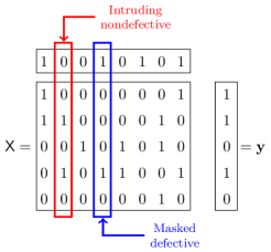
Figure 1: An example of a group testing problem, including a masked defective and an intruding non-defective, in the terminology we introduce here. The masked defective never appears in a positive test without some other defective item also being present. The intruding non-defective never appears in a negative test.

Notice that steps 1 and 2 in the DD algorithm make no mistake; indeed, step 1 just isolates all items that are ND, which can then be ignored, thus allowing us to restrict our attention to the items in ${\mathcal{PD}}$. The set ${\mathcal{PD}}$ contains the $K$ true defectives, plus a (random) number $G$ of intruding non-defectives (see Figure 1), meaning we can analyse the $T\times(K+G)$ submatrix ${\mathsf{S}}$, corresponding to the items in ${\mathcal{PD}}$. Step 2, in turn, isolates the definitely defective items of ${\mathcal{PD}}$, i.e. those defectives that appear with no other item of ${\mathcal{PD}}$. After step 2 we are then left with

• $G$ intruding non-defectives that haven’t been discarded in step 1;

• defectives that never appear without other ${\mathcal{PD}}$ items in a test (we call such an item masked – see Figure 1).

Hence only step 3 can make a mistake, which occurs when there are masked defectives which are erroneously declared to be non-defective. In other words, the DD algorithm can only make false-negative errors, and never makes false-positive errors, so $\widehat{\mathcal{K}}_{{\tt DD\;}\!\!}\subseteq\mathcal{K}$.

The motivation for Step 3 of the DD algorithm comes from the sparsity of the defective set. That is, we cannot be sure whether items in ${\mathcal{PD}}$ but not ${\mathcal{DD}}$ are defective or not. However, since defectiveness is assumed to be rare, in that $K\ll N$, it seems natural to assume that these items are nondefective, in the absence of evidence to the contrary. Conversely, the COMP algorithm assumes that these unknown items are defective, thereby often making false positive errors.

We derive an exact expression for the error probability of the DD algorithm in Section A.3. The main difference between the DD algorithm and the COMP algorithm of Chan et al. [6] is that COMP succeeds if and only if $G=0$, whereas DD can succeed for positive $G$.

3.3 The SCOMP algorithm

In order to improve on the DD algorithm of Section 3.2 we introduce the SCOMP (Sequential COMP) algorithm. The key observation is that $\widehat{\mathcal{K}}_{{\tt DD\;}\!\!}$ need not be a satisfying set, since there may exist positive tests which contain no elements of $\widehat{\mathcal{K}}_{{\tt DD\;}\!\!}$.

Definition 3.2.

Given an estimate $\widehat{\mathcal{K}}$, we say that a positive test is unexplained by $\widehat{\mathcal{K}}$ if it contains no element from $\widehat{\mathcal{K}}$.

Note that a set $\widehat{\mathcal{K}}\subseteq{\mathcal{PD}}$ of possible defectives being a satisfying set is equivalent to there being no unexplained positive tests.

Since each unexplained test must contain at least one of the masked defectives in $\mathcal{K}\setminus\widehat{\mathcal{K}}_{{\tt DD\;}\!\!}$, we might consider items in ${\mathcal{PD}}$ that appear in many unexplained tests as most likely to be defective. The SCOMP algorithm uses this principle to sequentially and greedily extend $\widehat{\mathcal{K}}_{{\tt DD\;}\!\!}$ to a satisfying set, by seeking items which explain the most currently unexplained tests. This is an attempt to exploit all the information available at each step, which is updated every time an item in ${\mathcal{PD}}$ is added to $\widehat{\mathcal{K}}$.

The algorithm proceeds as follows:

1. Carry out the first two steps of the DD algorithm; that is, generate an initial estimate $\widehat{\mathcal{K}}=\widehat{\mathcal{K}}_{{\tt DD\;}\!\!}={\mathcal{DD}}$, for ${\mathcal{DD}}$ as defined in (5).

2. Given an estimate $\widehat{\mathcal{K}}$:

   1. If $\widehat{\mathcal{K}}$ is satisfying, terminate the algorithm, and use $\widehat{\mathcal{K}}$ as our final estimate of $\mathcal{K}$.

   2. If $\widehat{\mathcal{K}}$ is not satisfying, then find the element $i\in{\mathcal{PD}}$ which appears in the largest number of tests which are unexplained by $\widehat{\mathcal{K}}$ (breaking ties arbitrarily), and create a new estimate $\widehat{\mathcal{K}}_{\rm new\!\!}=\widehat{\mathcal{K}}\bigcup\{i\}$. Repeat Step 2.

Notice that Step 2 gives an iterative procedure which greedily extends any estimate $\widehat{\mathcal{K}}$ to a satisfying set. The SCOMP algorithm is hard to analyse theoretically. However in Section 5 we give evidence from simulations that it outperforms the DD algorithm which it is based on, and gives performance very close to optimal.

It is interesting to notice the analogy with Chvatal’s approximation algorithm to the set covering problem (or just ‘set cover’) – see [28] for a discussion. Given a set $U$ and a family of subsets $S\subseteq{\mathcal{P}}(U)$, set cover requires us to find the smallest family of subsets in $S$ whose union contains all elements of $U$. This optimisation problem is NP-hard, as for a putative solution optimality cannot be verified in polynomial time. In 1979, Chvatal [8] proposed an approximate solution by choosing, at each stage, the set in $S$ that covers the most uncovered elements. The algorithm produces a solution which can be at most $H(|U|)$ times larger than the optimal, where $H(n)\sim\ln n$ is the $n$-th harmonic number. Similarly, SCOMP chooses defective items in a greedy manner to ‘cover’ (or in our terminology, ‘explain’) as many tests as possible, until all tests are explained. So similarly, we are guaranteed to find a satisfying set with no more than $KH(K)\sim K\ln K$ items.

Note that this implies that if the test design $\mathsf{X}$ is $KH(K)$-separable (see Definition 2.2), then the there will be only one satisfying set constaining $KH(K)$ or fewer items. Since SCOMP finds such a satisfying set, in this situation it is guaranteed to find the correct defective set $\mathcal{K}$. As before, though, we note that SCOMP can succeed even when $KH(K)$-separability is not achieved.

There are inapproximability results that accompany Chvatal’s algorithm, showing that, under standard complexity theory assumptions, no better approximation ratio is possible for set cover (see for example [28, Theorem 29.31]). In the light of this, we might consider SCOMP to similarly be a ‘best possible practical approximation’ to the SSS algorithm below.

3.4 Smallest satisfying set – SSS algorithm

We now consider what an optimal detection algorithm might look like, without worrying about its computational feasibility.

Facts we know for sure about the true defective set $\mathcal{K}$ are:

• $\mathcal{K}$ is a satisfying set, since we are considering noiseless testing,

• $K=|\mathcal{K}|$ is likely to be small, since we are considering regimes where $K\ll N$.

This suggests an approach where we attempt to find the smallest set that satisfies the outputs. (This approach is similar to that taken in compressed sensing, where one typically seeks the sparsest signal $\mathbf{x}$ that fits some given measurements $\mathbf{y}=\mathsf{A}\mathbf{x}$.)

That is, if we let $\mathbf{z}$ be a solution to the $\mathtt{0}$–$\mathtt{1}$ linear program

$$\begin{split}\text{minimize}\qquad&\mathbf{1}^{\top}\mathbf{z}\\ \text{subject to}\qquad&\mathbf{x}_{t}\cdot\mathbf{z}=0\quad\text{for $t$ with $y_{t}=\mathtt{0}$}\\ &\mathbf{x}_{t}\cdot\mathbf{z}\geq 1\quad\text{for $t$ with $y_{t}=\mathtt{1}$}\\ &\mathbf{z}\in\{\mathtt{0},\mathtt{1}\}^{N},\end{split}$$ (6)

then the smallest satisfying set SSS algorithm uses $\widehat{\mathcal{K}}_{{\tt SSS\;}\!\!}=\{i:z_{i}=\mathtt{1}\}$. (If there is not a unique solution to (6), choose one of the solutions arbitrarily.) We analyse the success probability of the SSS algorithm in Section A.5.

Note that if the number of defectives $K$ is known, we can add the constraint $\mathbf{1}^{\top}\mathbf{z}\geq K$ to ensure we find a satisfying set of size exactly $K$. In this situation, the SSS algorithm finds an arbitrary satisfying set of the correct size, and since we are considering noiseless testing, one can do no better than this, so SSS is optimal. Hence, for the unknown-$K$ setting we consider in this paper, we will often refer to SSS as ‘essentially optimal’.

Furthermore, notice that if the test design $\mathsf{X}$ is $K$-separable (see Definition 2.2), then the defective set is also the smallest satisfying set. Indeed, $K$-separability implies that no two sets of columns of $\mathsf{X}$ of size at most $K=|\mathcal{K}|$ have the same boolean sum, meaning that no other set as sparse as $\mathcal{K}$ or sparser than $\mathcal{K}$ could lead to the same outcome $\mathbf{y}$.

Unfortunately $\mathtt{0}$–$\mathtt{1}$ linear programming is NP-hard, so the SSS algorithm is unlikely to be feasible for large problems. We include it here as a ‘best possible’ benchmark against which to compare other more feasible algorithms.

However, for moderately sized problems, we can use our new DD algorithm as a preprocessing step to reduce the size of the program (6). Specifically, we can set

$$\mathcal{N}^{*} :=\mathcal{N}\setminus(\mathcal{ND}\cup{\mathcal{DD}}),$$

$$\mathcal{T}^{*} :=\{t\in\{1,\ldots,T\}:x_{it}=\mathtt{0}\text{ for all $i\in{\mathcal{DD}}$, and }y_{t}=\mathtt{1}\},$$

$$\mathsf{X}^{*} :=(x_{it}:i\in\mathcal{N}^{*},t\in\mathcal{T}^{*});$$

find $\mathbf{z}^{*}=(z_{i}^{*}:i\in\mathcal{N}^{*})$ to solve the smaller problem

minimize $$\mathbf{1}^{\top}\mathbf{z}^{*}$$

subject to $$\mathsf{X}^{*}\mathbf{z}^{*}\geq\mathbf{1}$$

$$\mathbf{z}^{*}\in\{\mathtt{0},\mathtt{1}\}^{|\mathcal{N}^{*}|};$$

and choose

$$\widehat{\mathcal{K}}_{{\tt SSS\;}\!\!}={\mathcal{DD}}\cup\{i\in\mathcal{N}^{*}:z_{i}^{*}=\mathtt{1}\}.$$

If the number of ‘not definitely anything’ items $|\mathcal{N}^{*}|$ is only of order $\ln N$, then the complexity of this problem becomes only polynomial in $N$, and could be regarded as practical.

We also mention that recent work by Malyutov and coauthors [18, 23] has tried to construct the defective set from the solution to the relaxed problem

minimize $$\mathbf{1}^{\top}\mathbf{z}$$

subject to $$\mathbf{x}_{t}\cdot\mathbf{z}=0\quad\text{for $t$ with $y_{t}=\mathtt{0}$}$$ (7)

$$\mathbf{x}_{t}\cdot\mathbf{z}\geq 1\quad\text{for $t$ with $y_{t}=\mathtt{1}$}$$ (8)

$$\mathbf{z}\geq\mathbf{0}$$

where the $z_{i}$ can be any positive real numbers. Chan et al. [7] consider a similar relaxed linear program for noisy group testing.

4 Bounds on rates

In this section, we give the main results of this paper. Below, we state bounds on the maximal achievable rates (recall Definition 2.7) of our algorithms with Bernoulli test designs. The bounds are illustrated in Figure 2.

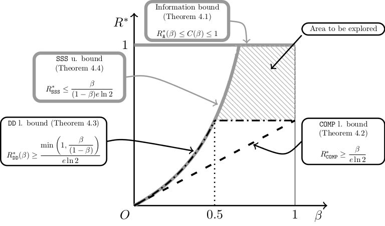
Figure 2: Bounds on achievable rates of the algorithms COMP, DD, and SSS for Bernoulli test designs, shown with the information bound on capacity.

First, from a simple counting argument, we have the following capacity bound, which we refer to as the information bound.

Theorem 4.1.

For any algorithm $\mathtt{A}$, we have $R^{*}_{\mathtt{A}}(\beta)\leq C(\beta)\leq 1$.

For a formal proof with explicit bounds on error probability, see for example [6] or [4]. The paper [4] proves strong error bounds (see Equation (9)), corresponding to a ‘strong converse’ in information theory.

Second, simple manipulation of Theorem A.2, a bound on the error probability of COMP  due to Chan et al [6, 7], gives the following rate bound:

Theorem 4.2.

For the COMP algorithm with a Bernoulli$(1/K)$ test design, we have

$$R^{*}_{\text{{COMP}}}\geq\frac{\beta}{e\ln 2}\approx 0.53\beta.$$

We give an alternative proof of Theorem A.2 in Remark A.5, and prove Theorem 4.2 in Appendix B.2.

For our new DD algorithm we have the following lower bound on rate.

Theorem 4.3.

For the DD algorithm with a Bernoulli$(1/K)$ test design, we have

$$R^{*}_{\text{{DD}}}\geq\frac{1}{e\ln 2}\min\left\{1,\frac{\beta}{1-\beta}\right\}\approx 0.53\min\left\{1,\frac{\beta}{1-\beta}\right\}.$$

In Appendix A.3 we give an exact expression for the error probability of DD; in Appendix A.4 we bound this expression, giving an easier-to-use approximation; and in Appendix B.3 we convert this into the above rate bound.

Comparing Theorems 4.2 and 4.3, we see that for $0<\beta<1$, the performance guarantees for DD strictly exceed those for COMP.

Finally, for the SSS  algorithm, we have the following upper bound on rate. Since SSS  is essentially optimal for Bernoulli tests, we argue that our new detection algorithms should be compared with this as the limit of what may be possible with Bernoulli test designs.

Theorem 4.4.

For the SSS algorithm with any Bernoulli test design, we have

$$R^{*}_{\text{{SSS}}}\leq\frac{1}{e\ln 2}\frac{\beta}{1-\beta}\approx 0.53\frac{\beta}{1-\beta}.$$

In Appendix A.6 we give a upper bound on the success probability of the SSS algorithm, which in Appendix B.4 we convert to the upper bound on rate of Theorem 4.4. We also give an lower bound on the success probability of the SSS algorithm, in Appendix A.5.

From Theorems 4.3 and 4.4, we see that the DD algorithm achieves the same rate as SSS for $\beta\leq\frac{1}{2}$, and hence is essentially optimal in this regime. We note also that for

$$\beta\leq\frac{e\ln 2}{1+e\ln 2}\approx 0.65,$$

the rate of the SSS algorithm is bounded away from the information bound $C(\beta)\leq 1$, which is achievable for adaptive testing [4]. There are two possible explanations for this. One is that Bernoulli tests are suboptimal in these regimes – and very far from optimal in the denser cases. The other is that there is an ‘adaptivity gap’, and no nonadaptive algorithms can perform as well adaptive algorithms here, with a gap that increases as the problem becomes denser.

Unfortunately, the complicated sequential nature of SCOMP makes it difficult to analyse mathematically. However, simulations in Section 5 show that in practice SCOMP performs better than DD. Hence, we conjecture that

$$R^{*}_{\mathtt{SCOMP}}\begin{cases}=\displaystyle\frac{1}{e\ln 2}\frac{\beta}{1-\beta}&\text{for $\beta\leq\frac{1}{2}$,}\\ \geq\displaystyle\frac{1}{e\ln 2}&\text{for $\beta>\frac{1}{2}$.}\end{cases}$$

The proofs of these theorems is sometimes quite involved, and we save details for the appendices. In Appendix A, we prove explicit bounds on the error probability of DD and SSS. In Appendix B we convert the error probability bounds into the bounds on achievable rates we see above. In Appendix C, we summarize some elementary probability facts we will use.

5 Simulations

In this section, we run simulations of our new algorithms, and compare our theoretical bounds to empirical results. All simulations were run with $N=500$ items, of which $K=10$ were defective (except for Figure 5), and Bernoulli test matrices with parameter $p=1/K$. Each plotted point is based on the average success rate from $1000$ simulations.

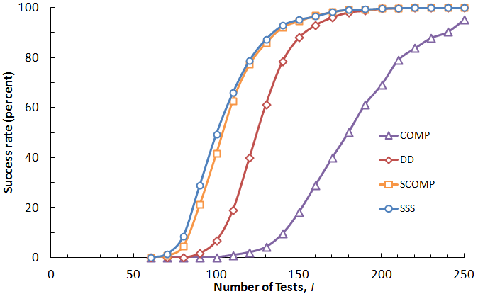
Figure 3: Performance of the COMP, DD, SCOMP and SSS algorithms for noiseless group testing with a Bernoulli test design with $N=500$, $K=10$, $p=1/10$.

Figure 3 shows the performance of the algorithms featured in this paper. Our DD algorithm far outperforms the COMP algorithm of Chan et al., and our SCOMP algorithm is better still. For this moderately sized example ($N=500$, $K=10$, $T\approx 100$), it was possible to use an integer linear programming solver to run the SSS algorithm (even without the improvement we mention in Section 3.4). Promisingly, the computationally simple SCOMP algorithm has performance very close to that of the essentially optimal but computationally hard SSS algorithm; the performance is particularly close in the most important high success probability regime.

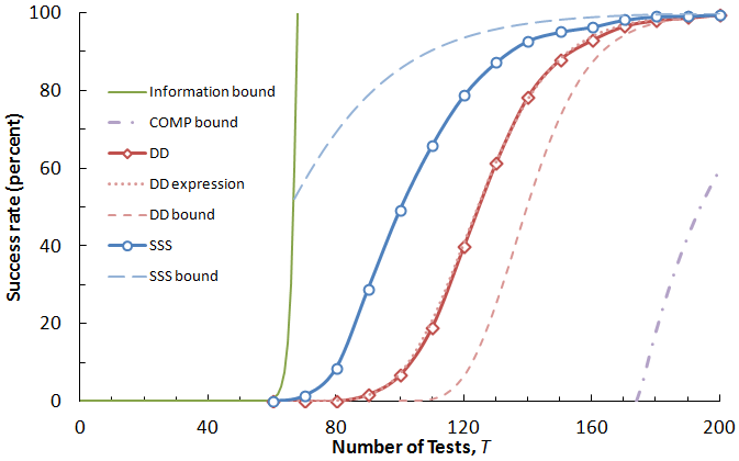
Figure 4: Performance of the DD and SSS algorithms, with the information lower bound (Theorem A.1), the COMP lower bound (Corollary B.2) of Chan et al., our exact expression for DD (Theorem A.4), our DD lower bound (see (28) in Lemma A.8), and our SSS upper bound (Theorem A.11) for noiseless group testing with a Bernoulli test design with $N=500$, $K=10$, $p=1/10$.

Figure 4 shows the performance of the DD algorithm. The algorithm does indeed perform as predicted analytically, and our bound is reasonably tight, especially in the high success probability regime. Note also that our bound on success probability is a big improvement on the Chan et al. bound for the COMP algorithm. While performance of DD is far from the information theoretic bound, the essentially optimal SSS algorithm shows that the bound is very far from achievable with a Bernoulli test design and $K$ unknown.

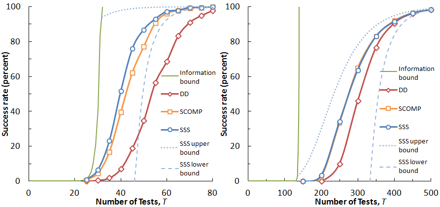
Figure 5: Performance of the SSS algorithm and associated bounds (Theorems A.1, A.9 and A.11) and the SCOMP algorithm for noiseless group testing with a Bernoulli test design with $N=500$ in a sparse case (left: $K=4$, $p=1/4$, $\beta_{{\rm eff}}=0.7769)$ and a dense case (right: $K=25$, $p=1/25$, $\beta_{{\rm eff}}=0.4820$.)

Figure 5 illustrates the difference between a sparse case (left subfigure) and dense case (right subfigure) of group testing. In the sparse case, our SSS upper bound is generally loose compared to the information bound, while the lower bound is generally right, especially in the high success rate regime. Here, the SCOMP algorithm slightly underperforms the more computationally difficult SSS algorithm. In the dense case, on the other hand, our SSS upper bound is much tighter than the information bound, while the lower bound is fairly loose away from the high success rate regime. Here, the SCOMP algorithm performs essentially equivalently to the difficult SSS algorithm, and even DD performs close to the SSS .

We can understand the performance illustrated in Figure 5 in terms of the rate results of Appendix B. In particular, given $N$ and $K$, we write $\beta_{{\rm eff}}=1-\ln K/\ln N$ for the value such that $K=N^{1-\beta_{{\rm eff}}}$. The sparse case has the value $\beta_{{\rm eff}}=0.7769$, and corresponds to the region $\beta>1/2$ where the rate bounds are less tight and the DD algorithm is probably not optimal. In contrast, the denser case has $\beta_{{\rm eff}}=0.4820$ and corresponds to the region $\beta<1/2$ where the DD algorithm asymptotically converges to the SSS bound.

6 Conclusions and further work

We have introduced several new algorithms for noiseless non-adaptive group testing, including the DD algorithm and SCOMP algorithm. We have demonstrated by bounds on their maximum achievable rates and by direct simulation that they perform well compared with known algorithms in the literature, and in some denser cases are asymptotically optimal.

We briefly mention some problems for future work:

1. To give asymptotic bounds on the performance of the SSS algorithm, which would require a more detailed combinatorial analysis. Such asymptotic bounds would allow us to deduce tighter bounds on the value of $C(\beta)$ for $\beta>1/2$.

2. To compare the performance of algorithms under Bernoulli test designs and other matrix designs, including the LDPC-inspired designs of Wadayama [29].

3. To develop similar algorithms and bounds for the noisy case.

Appendix A Proofs: bounds on error probability

A.1 Information bound

For comparison, we note the information bound in a form due to Baldassini, Johnson and Aldridge [4, Theorem 3.1]:

Theorem A.1 ([4]).

Consider testing a set of $N$ items with $K$ defectives. Any algorithm to recover the defective set with $T$ tests has success probability satisfying

$${\mathbb{P}}({\rm success})\leq\frac{2^{T}}{\binom{N}{K}}.$$ (9)

This theorem strengthened a result of Chan et al.  [6, Theorem 1], who referred to their bound as ‘folklore’, noting that similar bounds appear in the literature, such as [13].

A.2 COMP 

Chan et al. [6, equation (8)][7, equation (34)] give the following bound on the success probability of the COMP algorithm:

Theorem A.2.

For noiseless group testing with a Bernoulli$(p)$ test design, the success probability of the COMP algorithm is bounded by

$${\mathbb{P}}({\rm success})\geq 1-(N-K)\big{(}1-p(1-p)^{K}\big{)}^{T}.$$ (10)

By differentiation, it is easy to see that (10) is maximised at $p=1/(K+1)$, agreeing with Johnson and Sejdinovic’s argument that $p=1/K$ is asymptotically optimal in the $\lim_{K\to\infty}\lim_{N\to\infty}$ regime [26]. Note that we show in Remark A.5 below that Theorem A.2 can be recovered using our techniques.

A.3 DD: exact expression

We now derive an exact expression for the probability that the DD algorithm recovers the defective set exactly. It is helpful to mentally sort the rows and columns of the testing matrix $\mathsf{X}$ (and outcome vector $\mathbf{y}$) in a suitable way; this implies no loss of generality. This is illustrated in Figure 6.

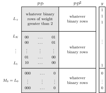
Figure 6: The testing matrix $\mathsf{X}$, where the rows have been grouped according to the partition ${\mathbf{L}}$ and the columns into the two subsets ${\mathcal{PD}}$ and ${\mathcal{PD}}^{\complement}$. The shaded area is the submatrix ${\mathsf{S}}$. Notice that the variables $L_{0},\ldots,L_{+}$ do not index single rows but groups of rows, according to the definition of ${\mathbf{L}}$ (11).

Recall from Definition 3.1 that we write ${\mathcal{PD}}=\mathcal{ND}^{\complement}$ for the set of possible defectives (items which do not appear in any negative test). It will also be convenient here to, without loss of generality, label the actual $K$ defectives as $\mathcal{K}=\{1,2,\dots,K\}$. Note that $\mathcal{K}\subseteq{\mathcal{PD}}$, and the only type of error we can make is a false negative, when a defective item is masked. It will be useful to consider the following partition of the number of tests $T$, which depends on the random matrix $\mathsf{X}$ and the defective set $\mathcal{K}$:

$$L_{0} =\text{$\#$ tests with no defective items in,}$$

$$L_{i} =\text{$\#$ tests containing $i$ and no other element of ${\mathcal{PD}}$, for $i=1,\ldots,K$,}$$ (11)

$$L_{+} =\text{$\#$ remaining tests.}$$

If $L_{i}\neq 0$ for some $i\in\mathcal{K}$ then the DD algorithm correctly identifies the defective element $i$. Thus the success probability of the DD algorithm is precisely the probability that $L_{i}\neq 0$ for all $i\in\mathcal{K}$

$${\mathbb{P}}({\rm success})={\mathbb{P}}\left(L_{1}\neq 0,\dots,L_{K}\neq 0\right).$$ (12)

For this reason, we want to know the distribution of $\mathbf{L}=(L_{0},L_{1},\dots,L_{K},L_{+})$. Unfortunately the distribution of $\mathbf{L}$ is quite complicated, but we will be able to analyse it conditioned on the number of possible defectives $|{\mathcal{PD}}|=K+G$ and a related random vector $\mathbf{M}$. Recall from Section 3.2 that $G$ is the number of nondefective items that are nonetheless in ${\mathcal{PD}}$. We define $\mathbf{M}=(M_{0},M_{1},\dots,M_{K},M_{+})$ as follows:

$$M_{0} =\text{$\#$ tests with no defective items in,}$$

$$M_{i} =\text{$\#$ tests with $i$ the only defective item in, for $i=1,\ldots,K$}$$

$$M_{+} =\text{$\#$ tests with two or more defective items in.}$$

Note that this is similar to the definition of $\mathbf{L}$, but with the set of possible defectives ${\mathcal{PD}}$ replaced by the set of actual defectives $\mathcal{K}$. Write

$$q_{0} ={\mathbb{P}}(\text{no defectives})=(1-p)^{K},$$

$$q_{1} ={\mathbb{P}}(\text{$1$ the only defective})=p(1-p)^{K-1},$$

$$q_{+} ={\mathbb{P}}(\text{two or more defectives})=1-q_{0}-Kq_{1},$$

$${\mathbf{q}} =(q_{0},\underbrace{q_{1},\dots,q_{1}}_{\text{$K$ terms}},q_{+}).$$

The following lemma then holds:

Lemma A.3.

Using a Bernoulli$(p)$ test design, ${\mathbf{M}}=(M_{0},M_{1},\dots,M_{K},M_{+})$ is multinomial with probability distribution ${\mathbb{P}}_{T;{\mathbf{q}}}$ defined as

$${\mathbb{P}}_{T;{\mathbf{q}}}(m_{0},m_{1},\ldots,m_{k},m_{+})=\displaystyle{\frac{T!}{m_{+}!\prod_{i=0}^{K}m_{i}!}}q_{0}^{m_{0}}q_{1}^{m_{1}+\cdots+m_{k}}q_{+}^{m_{+}}\ ,$$ (13)

for $\sum_{i=0}^{K}m_{i}+m_{+}=T$.

By analysing the relationship between ${\mathbf{M}}$ and ${\mathbf{L}}$, we are able to give the probability of success of the DD algorithm. The strategy is as follows: from (13) we have the distribution of $\mathbf{M}$; given $\mathbf{M}$, (16) below gives the distribution of $G$; given $\mathbf{M}$ and $G$, (18) gives the distribution of $L$; and given the distribution of $L$, we have from (12) the probability of success.

Putting this all together, we can derive an exact expression for the success probability of the DD algorithm, in terms of the binomial mass function $b(k;n,t):=\binom{n}{k}t^{k}(1-t)^{n-k}$ and $\phi_{K}$, defined as

$$\phi_{K}(q,T):=\sum_{\ell=0}^{K}(-1)^{\ell}\binom{K}{\ell}(1-\ell q)^{T}\ ,\mbox{\;\;\; for $q\in[0,1]$.}$$ (14)

Appendix C summarises some well-known results from probability theory, including properties of the multinomial distribution. In particular, Lemma C.2 shows that $\phi_{K}$ gives the probability of a set of components of a multinomial being non-zero, in a certain symmetric situation.

Theorem A.4.

Given a Bernoulli$(p)$ test design, the success probability of the DD algorithm is

$${\mathbb{P}}({\rm success})=\sum_{m_{0}=0}^{T}\sum_{g=0}^{N-K}b(m_{0};T,q_{0})b(g;N-K,(1-p)^{m_{0}})\Phi_{K}(g,m_{0})\ ,$$ (15)

where we write $\Phi_{K}(g,m_{0})=\phi_{K}\left(q^{*}(g),T-m_{0}\right)$ for $q^{*}(g)=q_{1}(1-p)^{g}/(1-q_{0})$ .

Proof.

The key is to condition on the value of $M_{0}$. By Lemma C.1.2, $M_{0}\sim{\rm Bin}(T,q_{0})$, and by Lemma C.1.3, conditioned on $M_{0}=m_{0}$, the vector ${\mathbf{M}}^{\prime}=(M_{1},\ldots,M_{k},M_{+})\sim{\mathbb{P}}_{T-m_{0};{\mathbf{q}}^{\prime}}$, where

$${\mathbf{q}}^{\prime}=\left(\frac{q_{1}}{1-q_{0}},\ldots,\frac{q_{1}}{1-q_{0}},\frac{q_{+}}{1-q_{0}}\right).$$

Next, given $M_{0}$, we can find the distribution of $G$, the number of intruding non-defectives. First, all $K$ actual defectives will be in ${\mathcal{PD}}$. Then each of the other $N-K$ items will fail to be in any of the $M_{0}$ negative tests with probability $(1-p)^{M_{0}}$. Hence we have that, independent of ${\mathbf{M}}^{\prime}$, the conditional distribution of $G$ given $M_{0}$ is

$$G\mid M_{0}\sim\text{Bin}(N-K,(1-p)^{M_{0}}).$$ (16)

We will express the success probability as

$${\mathbb{P}}({\rm success})=\sum_{m_{0}=0}^{T}\sum_{g=0}^{N-K}b(m_{0};T,q_{0})b(g;N-K,(1-p)^{m_{0}}){\mathbb{P}}({\rm success}\mid M_{0}=m_{0},G=g).$$ (17)

Next, given $\mathbf{M}$ and $G$, we can write down the conditional distribution of $\mathbf{L}$, since for $i=1,\ldots,K$,

$$L_{0} =M_{0},$$

$$L_{i}\mid M_{i},G \sim\text{Bin}(M_{i},(1-p)^{G}),$$ (18)

$$L_{+} =T-\sum_{i=0}^{K}L_{i}.$$

This is because for each $i$, a test which contains defective item $i$ and no other defective will contribute to $M_{i}$. However, it will only contribute to $L_{i}$ if it also contains none of the $G$ intruding non-defectives. The Bernoulli sampling of the matrix $\mathsf{X}$ means that each such test will contribute to $L_{i}$ independently with probability $(1-p)^{G}$. Equivalently, the $L_{i}$ are independently thinned versions of $M_{i}$ (in the sense of Rényi [24]), with thinning parameter $(1-p)^{G}$.

Repeatedly using Lemma C.1.4, we can deduce that, conditional on $M_{0}=m_{0}$ and $G=g$, we have that

$$(L_{1},L_{2},\ldots,L_{k},M_{1}-L_{1},\ldots,M_{k}-L_{k},M_{+})\sim{\mathbb{P}}_{T-m_{0},{\mathbf{q}}^{\prime\prime}},$$

where

$${\mathbf{q}}^{\prime\prime}=\Big{(}\frac{q_{1}(1-p)^{g}}{1-q_{0}},\ldots,\frac{q_{1}(1-p)^{g}}{1-q_{0}},\frac{q_{1}(1-(1-p)^{g})}{1-q_{0}},\ldots,\frac{q_{1}(1-(1-p)^{g})}{1-q_{0}},\frac{q_{+}}{1-q_{0}}\Big{)}.$$

From (12), we know that the DD algorithm will be successful precisely in the event $\bigcap_{i=1}^{K}\{L_{i}\neq 0\}$. Lemma C.2 gives an exact expression for this probability as

$${\mathbb{P}}({\rm success}|M_{0}=m_{0},G=g)=\phi_{K}\left(\frac{q_{1}(1-p)^{g}}{1-q_{0}},T-m_{0}\right).$$

We can then directly substitute this in (17) to deduce the theorem. ∎

Remark A.5.

We can recover the bound (10) of Chan et al. [6] using our techniques. As previously remarked in Section 3.2, their COMP algorithm succeeds if and only if $G=0$. Using (16) we know that $G\mid M_{0}\sim\text{Bin}(N-K,(1-p)^{M_{0}})$. This means that

$${\mathbb{P}}({\rm success}) =\sum_{m_{0}=0}^{T}{\mathbb{P}}(M_{0}=m_{0}){\mathbb{P}}(G=0|M_{0}=m_{0})$$

$$=\sum_{m_{0}=0}^{T}\binom{T}{m_{0}}q_{0}^{m_{0}}(1-q_{0})^{T-m_{0}}\left((1-(1-p)^{m_{0}})^{N-k}\right)$$ (19)

$$\geq\sum_{m_{0}=0}^{T}\binom{T}{m_{0}}q_{0}^{m_{0}}(1-q_{0})^{T-m_{0}}\left(1-(N-k)(1-p)^{m_{0}}\right)$$

$$=1-(N-k)\left(q_{0}(1-p)+1-q_{0})\right)^{T}.$$

Here we bound the bracketed term (19) using the Bernoulli inequality

$$(1+x)^{T}\geq 1+xT\mbox{ for all $x\geq-1$ and $T\geq 0$,}$$ (20)

and the result follows since $q_{0}=(1-p)^{k}$, so that $q_{0}(1-p)+1-q_{0}=1-p(1-p)^{k}$.

A.4 DD: bounds

Theorem A.4 gives a complicated multipart expression that gives the success probability of the DD algorithm. In fact, since $\Phi_{K}$ is defined in terms of a summation formula, the expression (15) is a triple sum, which is difficult to analyse and control.

Notice that for the success probability we can use the bound $\phi_{K}(q,T-m_{0})\geq\max\{0,1-K(1-q)^{T-m_{0}}\}$ (see Lemma C.2) to reduce the equality (17) to a lower bound, expressed in terms of a double sum. In this subsection we derive a simpler bound on the success probability. We repeatedly use the fact that

$$(1-x)^{y}\leq\exp(-xy)\mbox{\;\;\; for $0\leq x\leq 1$ and $y\geq 0$.}$$ (21)

In order to analyse the success probability of the DD algorithm, it is useful to bound $q_{0}$ and $q_{1}$.

Lemma A.6.

Writing $p=1/K$, and defining $q_{0}=(1-p)^{K}$ and $q_{1}=p(1-p)^{K-1}$, we notice that $q_{1}=q_{0}/(K-1)$. Hence for $K\geq 2$ we deduce that:

$$\frac{K-2}{K-1}e^{-1} \leq q_{0}\leq e^{-1},$$ (22)

$$\frac{q_{1}}{1-q_{0}} \leq\frac{1}{K}.$$ (23)

Proof.

The upper bound of (22) follows by taking $x=p$ and $y=K$ in (21) above. The lower bound is slightly more involved; taking $x=-p/(1-p)$ and $y=K$, we deduce from (21) that $(1-p)^{K}\geq\exp(-1-\frac{1}{K-1})$. Further, taking $x=p/(1-p)$ and $y=1$ in (21) tells us that $\exp(-\frac{1}{K-1})\geq\frac{K-2}{K-1}$, and the result follows.

Further, Equation (23) follows on rearranging the fact that $q_{0}+Kq_{1}\leq 1$. ∎

We bound $\Phi_{K}$, using arguments based on the Bernoulli inequality (as previously used in Remark A.5).

Lemma A.7.

For fixed $T$, $K$ and $n_{0}$, taking

$$q^{*}(g):=\frac{q_{1}(1-p)^{g}}{1-q_{0}}=\frac{p(1-p)^{K+g-1}}{1-(1-p)^{K}},$$

the function

$$\Phi_{K}(g,m_{0}) = \phi_{K}(q^{*}(g),T-m_{0})$$ (24)

$$\geq \max\left\{0,1-K\exp\left(-\frac{q_{1}(T-m_{0})}{1-q_{0}}\right)\exp\left(\frac{pq_{1}(T-m_{0})}{1-q_{0}}g\right)\right\}.$$

Proof.

First observe that as in Lemma C.2 we can write

$$1-\Phi_{K}(g,m_{0})\leq K(1-q^{*}(g))^{T-m_{0}}\leq K\exp\left(-(T-m_{0})q^{*}(g)\right),$$ (25)

since (21) gives that $(1-x)^{y}\leq\exp(-xy)$ for $0\leq x\leq 1$ and $y\geq 0$. Further, the Bernoulli inequality (20), giving $(1+x)^{T}\geq 1+xT$, means that

$$q^{*}(g)=\frac{q_{1}(1-p)^{g}}{1-q_{0}}\geq\frac{q_{1}(1-pg)}{1-q_{0}},$$

and substituting this in (25), the result follows. ∎

We now prove a theorem to bound the success probability of the DD algorithm, by exploiting the favourable geometry of the distributions of $(M_{0},G)$ and $\Phi_{K}$, the probability that no defectives are masked. The strategy is that since $M_{0}$, the number of tests containing no defectives, is concentrated around its mean $Tq_{0}$, then bounding $\Phi_{K}$ will give a bound on the overall success probability, by controlling the inner sum in Theorem A.4.

Lemma A.8.

For any given $m_{0}$ we can bound the inner sum in Theorem A.4 by

$$\sum_{g=0}^{N-K}b(g;N-K,(1-p)^{m_{0}})\Phi_{K}(g,m_{0})\geq\max\left\{0,1-K\exp\Theta(T,m_{0})\right\},$$ (26)

where we write

$$\Theta(T,m_{0})=N(1-p)^{m_{0}}\left(\exp\left(\frac{(T-m_{0})pq_{1}}{1-q_{0}}\right)-1\right)-\frac{q_{1}(T-m_{0})}{1-q_{0}}.$$ (27)

Hence, given a Bernoulli$(p)$ test design, the probability of success under the DD algorithm satisfies

$${\mathbb{P}}({\rm success})\geq\sum_{m_{0}=0}^{T}b(m_{0};T,q_{0})\max\left[0,1-K\exp\left(\Theta(T,m_{0})\right)\right].$$ (28)

Proof.

Using Lemma A.7 we can simply bound the left-hand side by writing $\overline{p}=(1-p)^{m_{0}}$ and using the binomial theorem:

$$\sum_{g=0}^{N-K}\binom{N-K}{g}\overline{p}^{g}(1-\overline{p})^{N-K-g}\left[K\exp\left(-\frac{q_{1}(T-m_{0})}{1-q_{0}}\right)\exp\left(\frac{(T-m_{0})gpq_{1}}{1-q_{0}}\right)\right]$$

$$\qquad=K\exp\left(-\frac{q_{1}(T-m_{0})}{1-q_{0}}\right)\sum_{g=0}^{N-K}\binom{N-K}{g}\left(\overline{p}\exp\left(\frac{(T-m_{0})pq_{1}}{1-q_{0}}\right)\right)^{g}(1-\overline{p})^{N-K-g}$$

$$\qquad=K\exp\left(-\frac{q_{1}(T-m_{0})}{1-q_{0}}\right)\left(\overline{p}\exp\left(\frac{(T-m_{0})pq_{1}}{1-q_{0}}\right)+1-\overline{p}\right)^{N-k}$$

$$\qquad\leq K\exp\left((N-K)(1-p)^{m_{0}}\left(\exp\left(\frac{(T-m_{0})pq_{1}}{1-q_{0}}\right)-1\right)-\frac{q_{1}(T-m_{0})}{1-q_{0}}\right).$$ (29)

where the final inequality follows using $(1+x)^{y}\leq\exp(xy)$ for positive $x$ and $y$. ∎

A.5 SSS: lower bound

We have the following lower bound on the success probability of the SSS algorithm.

Theorem A.9.

For noiseless group testing with a Bernoulli($p$) test design, the success probability of the SSS algorithm is bounded by

$${\mathbb{P}}({\rm success})\geq 1-K\big{(}1-Q(K,K-1,K-1)\big{)}^{T}-\sum_{B=0}^{K-1}\binom{K}{B}\binom{N-K}{K-B}\big{(}1-Q(K,K,B)\big{)}^{T},$$ (30)

where we write

$$Q(K,L,B)=(1-p)^{K}+(1-p)^{L}-2(1-p)^{K+L-B}.$$ (31)

The final term in (30), which corresponds to the error probability when $K$ is known, has previously been analysed by Sebő [25] in the fixed $K$ regime (equivalent to our $\beta=1$).

To prove Theorem A.9 we will require the following lemma.

Lemma A.10.

The probability that a single Bernoulli($p$) test $\mathbf{x}$ gives a different outcome depending on whether the defective set is $\mathcal{K}$ or $\mathcal{L}$ is $Q(|\mathcal{K}|,|\mathcal{L}|,|\mathcal{K}\cap\mathcal{L}|)$, where $Q$ is as in (31).

Proof.

Write $K=|\mathcal{K}|$, $L=|\mathcal{L}|$, and $B=|\mathcal{K}\cap\mathcal{L}|$ for respectively the number of items in $\mathcal{K}$, in $\mathcal{L}$, and in both $\mathcal{K}$ and $\mathcal{L}$. Also write $q=1-p$.

The test gives a negative outcome with defective set $\mathcal{K}$ but a positive outcome with defective set $\mathcal{L}$ if and only if no items of $\mathcal{K}$ are included in the test, but at least one item $\mathcal{L}\setminus\mathcal{K}$ is included. This occurs with probability

$$q^{K}(1-q^{L-B})=q^{K}-q^{K+L-B}.$$

Similarly, the test gives a positive outcome with defective set $\mathcal{K}$ but a negative outcome with defective set $\mathcal{L}$ with probability

$$q^{L}(1-q^{K-B})=q^{L}-q^{K+L-B}.$$

Adding together the probabilities of these disjoint events gives the result. ∎

We can now prove Theorem A.9.

Proof.

The SSS algorithm may make an error if the true defective set $\mathcal{K}$ is not the unique smallest satisfying set. Thus the error probability of SSS is

$$\epsilon\leq{\mathbb{P}}\Bigg{(}\bigcup_{\begin{subarray}{c}|\mathcal{L}|\leq K\\ \mathcal{L}\neq\mathcal{K}\end{subarray}}A(\mathcal{L},\mathcal{K})\Bigg{)},$$

where $A(\mathcal{L},\mathcal{K})$ denotes the event that the sets $\mathcal{L}$ and $\mathcal{K}$ would give identical outcomes for all $T$ tests.

Consider a set $\mathcal{L}$ containing $|\mathcal{L}|=L$ items, where there are $B=|\mathcal{K}\cap\mathcal{L}|$ items in both $\mathcal{L}$ and $\mathcal{K}$. By Lemma A.10 and the fact that tests are independent, we have that

$${\mathbb{P}}\big{(}A(\mathcal{L},\mathcal{K})\big{)}=\big{(}1-Q(K,L,B)\big{)}^{T}$$

At this stage we can get a simple bound by using the union bound to write

$$\epsilon \leq\sum_{\begin{subarray}{c}|\mathcal{L}|\leq K\\ \mathcal{L}\neq\mathcal{K}\end{subarray}}{\mathbb{P}}\big{(}A(\mathcal{L},\mathcal{K})\big{)}$$

$$=\sum_{\begin{subarray}{c}|\mathcal{L}|\leq K\\ \mathcal{L}\neq\mathcal{K}\end{subarray}}\big{(}1-Q(K,|\mathcal{L}|,|\mathcal{K}\cap\mathcal{L}|)\big{)}^{T}$$

$$=\sum_{L=0}^{K}\sum_{B=0}^{L}\binom{K}{B}\binom{N-K}{L-B}\big{(}1-Q(K,L,B)\big{)}^{T}-1,$$ (32)

where the $-1$ is because our sum includes a term for $L=B=K$, corresponding to the true defective set.

However, we can get a tighter bound by noting that many of the events $A(\mathcal{K},\mathcal{L})$ are subsets of other events of the same type. First, given a satisfying set $\mathcal{L}$ with $B=L<K-1$ – that is, with no false positives and at least two false negatives – the event $A(\mathcal{K},\mathcal{L})\subset A(\mathcal{K},\mathcal{L}^{\prime})$ with $L^{\prime}=B^{\prime}=K-1$, where $\mathcal{L}^{\prime}$ is the set $\mathcal{L}$ with extra defective items added. Second, given a satisfying set $\mathcal{L}$ with $B<L<K$ – that is, with at least one false positive and at least one false negative – the event $A(\mathcal{K},\mathcal{L})\subset A(\mathcal{K},\mathcal{L}^{\prime\prime})$ with $L^{\prime\prime}=K$, where again $\mathcal{L}^{\prime\prime}$ is the set $\mathcal{L}$ with extra defective items added.

Considering only the terms in (32) with $L=B=K-1$ and the terms with $L=K$ gives the tighter bound

$$\epsilon\leq K\big{(}1-Q(K,K-1,K-1)\big{)}^{T}+\sum_{B=0}^{K-1}\binom{K}{B}\binom{N-K}{K-B}\big{(}1-Q(K,K,B)\big{)}^{T}$$

as desired. ∎

A.6 SSS: upper bound

Next, in Theorem A.11, we give an upper bound on the success probability of the SSS algorithm. As discussed in Section 3.4, this algorithm can be viewed as an idealized benchmark for the performance of any algorithm (when the number of defectives is unknown), so this bound should control the success probability of any algorithm.

Theorem A.11.

For any $K$, if we sample $\mathsf{X}$ according to a Bernoulli($p$) test design, then for any $p$, the SSS algorithm has success probability bounded above by

$${\mathbb{P}}({\rm success})\leq\phi_{K}\left(\frac{1}{e(K-1)},T\right),$$ (33)

Proof.

The key is to observe that if one of the defective items is masked by the other $K-1$ defectives, then the SSS algorithm will not succeed, since the $K-1$ items in question form a smaller satisfying set.

Equivalently, the set of matrices for which SSS succeeds is a subset of the matrices for which $M_{i}\neq 0$ for each defective $i$. This means that for any $p$, we can write

$${\mathbb{P}}({\rm success}) \leq {\mathbb{P}}\left(\bigcap_{i=1}^{K}\{M_{i}\neq 0\}\right)=\phi_{K}(p(1-p)^{K-1},T),$$

where the equality follows from Lemma C.2 below. Now, Lemma C.3 below shows that $\phi_{K}(q,T)$ is increasing in $q$. Observe that since $p(1-p)^{K-1}$ is maximised at $p=1/K$, for any $p$, (22) means we can write $p(1-p)^{K-1}\leq\frac{1}{K-1}e^{-1}$. ∎

It is interesting to note that the upper bound of Theorem A.11 is complementary to the universal upper bound of Theorem A.1. In particular, note that (33) does not depend on $N$, but only $K$. This means that which bound is tighter for a particular $K$ will depend on the overall sparsity of the problem.

Appendix B Proofs: bounds on achievable rates

B.1 A lemma for rate calculations

In order to carry out rate calculations, it is useful to have the following limit for normalized binomial coefficients:

Lemma B.1.

If $K=N^{1-\beta}$ then we can write

$$\lim_{N\rightarrow\infty}\frac{\log_{2}\binom{N}{K}}{K\ln N}=\frac{\beta}{\ln 2}.$$ (34)

Proof.

Well-known bounds on the binomial coefficients (see for example [17, Page 1097]) state that for any $K$, we have

$$\left(\frac{N}{K}\right)^{K}\leq\binom{N}{K}\leq\left(\frac{Ne}{K}\right)^{K}.$$ (35)

Taking logarithms to base 2 and dividing by $K\ln N$, using the fact that $N/K=N^{\beta}$, we obtain

$$\frac{K\beta\log_{2}N}{K\ln N}\leq\frac{\log_{2}\binom{N}{K}}{K\ln N}\leq\frac{K\beta\log_{2}N}{K\ln N}+\frac{\log_{2}e}{\ln N},$$

and the result follows on sending $N\to\infty$. ∎

B.2 COMP

Our new results can be contrasted with the following lower bound of Chan et al. [6, Theorem 4], which follows by rearranging the bound on success probability in Theorem A.2:

Corollary B.2.

For any $\delta>0$, using $T=e(1+\delta)K\ln N$ tests ensures that COMP has

$${\mathbb{P}}({\rm success})\geq 1-N^{-\delta}.$$

Hence we have

$$R^{*}_{\mathtt{COMP}}(\beta)\geq\frac{\beta}{e\ln 2},$$ (36)

which was Theorem 4.2 above.

B.3 DD

Theorem B.3.

Write $k(\beta)=\max\{\beta,1-\beta\}$ and fix $\delta>0$. Choosing $T=(k(\beta)+\delta)eK\ln N$ ensures that the success probability of the DD algorithm tends to 1 in the regime where $K=N^{1-\beta}$.

Proof.

First, we deduce that the quantity $\Theta(T,m_{0})$ defined in (27) can be bounded by the product of two terms. That is, for all $m_{0}$:

$$\Theta(T,m_{0}) \leq N\exp(-pm_{0})\left(\exp\left(\frac{(T-m_{0})pq_{1}}{1-q_{0}}\right)-1\right)-\frac{q_{1}(T-m_{0})}{1-q_{0}}$$

$$\leq\biggl{(}\frac{q_{1}(T-m_{0})}{1-q_{0}}\biggr{)}\biggl{(}Np\exp(-pm_{0})\exp\left(\frac{(T-m_{0})pq_{1}}{1-q_{0}}\right)-1\biggr{)}$$ (37)

Here, again, the first inequality uses the fact that (21) gives $(1-x)^{y}\leq\exp(-xy)$ for $0\leq x\leq 1$ and $y\geq 0$, and the last inequality follows using the fact that $\exp(x)-1\leq x\exp(x)$ for all $x$, and taking $x=(T-m_{0})pq_{1}/(1-q_{0})$.

For fixed $\epsilon:=\delta/6(\delta+k(\beta))$, we will separately bound the two bracketed terms of Equation (37) for $m_{0}\in\left(T(q_{0}-\epsilon/e),T(q_{0}+\epsilon/e)\right)$ in Equations (38) and (40) below.

We control the first term of (37), by bounding $m_{0}$ from below by $T(q_{0}-\epsilon/e)$ to deduce that (since $q_{1}=q_{0}/(K-1)$ as in Lemma A.6 above), for $K\geq 2$:

$$\frac{q_{1}(T-m_{0})}{1-q_{0}} \leq\frac{Tq_{0}}{K-1}\left(1+\frac{\epsilon}{e(1-q_{0})}\right)\leq\frac{T}{e(K-1)}\left(\frac{K-2}{K-1}+\frac{\epsilon}{e-1}\right)$$

$$=\ln N(k(\beta)+\delta)\left(\frac{K}{K-1}\left(\frac{K-2}{K-1}+\frac{\epsilon}{e-1}\right)\right)$$

$$\leq\ln N(k(\beta)+\delta)\left(1+2\epsilon\right)$$

$$=\ln N(k(\beta)+4\delta/3),$$ (38)

using the facts that (see (22)), $\frac{K-2}{K-1}e^{-1}\leq q_{0}\leq e^{-1}$, that function $t/(1-t)$ is increasing in $t$, and by the choice of $\epsilon$ given above. Similarly, by bounding $m_{0}$ from below by $T(q_{0}-\epsilon/e)$, we can express

$$-pm_{0}+\frac{(T-m_{0})pq_{1}}{1-q_{0}} \leq-pT(q_{0}-q_{1})+\frac{\epsilon pT}{e}\left(1+\frac{q_{1}}{1-q_{0}}\right)$$

$$\leq-pTq_{0}\frac{K-2}{K-1}+\frac{2\epsilon pT}{e}$$

$$\leq\left(\frac{pT}{e}\right)\left(-\left(\frac{K-2}{K-1}\right)^{2}+2\epsilon\right)$$

$$\leq\ln N(k(\beta)+\delta)(-1+3\epsilon)\mbox{ \;\;\;\;\; for $K$ sufficiently large }$$

$$=\ln N(-k(\beta)-\delta/2),$$ (39)

where we use the fact that (23) gives $\frac{q_{1}}{1-q_{0}}\leq\frac{1}{K}\leq 1$, the bound $\frac{K-2}{K-1}e^{-1}\leq q_{0}$ from (22), and the choice of $\epsilon$ given above. Hence, using the fact that $Np=N/K=N^{\beta}$, (39) gives that the second term of (37) can be bounded by

$$\biggl{(}Np\exp(-pm_{0})\exp\left(\frac{(T-m_{0})pq_{1}}{1-q_{0}}\right)-1\biggr{)} \leq N^{\beta-k(\beta)-\delta/2}-1\leq N^{-\delta/2}-1,$$ (40)

since $\beta\leq k(\beta)$. Hence, for $N$ sufficiently large and $m_{0}$ in this range, multiplying (38) and (40) gives $\Theta(T,m_{0})\leq\ln N(-k(\beta)-\delta)$. This means that (since $k(\beta)>1-\beta$) we can write

$$K\exp(\Theta(T,m_{0}))\leq N^{-\delta}.$$

Using Lemma A.8, we deduce that the success probability satisfies

$${\mathbb{P}}({\rm success}) \geq\sum_{m_{0}=0}^{T}b(m_{0};T,q_{0})\max\left[0,1-K\exp\left(\Theta(T,m_{0})\right)\right]$$

$$\geq\sum_{m_{0}=T(q_{0}-\epsilon)}^{T(q_{0}+\epsilon)}b(m_{0};T,q_{0})\left[1-K\exp\left(\Theta(T,m_{0})\right)\right]$$

$$\geq{\mathbb{P}}\biggl{(}T(q_{0}-\epsilon/e)\leq M_{0}\leq T(q_{0}+\epsilon/e)\biggr{)}(1-N^{-\delta}).$$

which converges to 1 by Chernoff’s inequality, Theorem C.4. ∎

We can now prove Theorem 4.3, that

$$R_{\mathtt{DD}}(\beta)\geq\frac{1}{e\ln 2}\min\left(1,\frac{\beta}{1-\beta}\right).$$

Proof of Theorem 4.3.

Theorem B.3 shows that for $K=N^{1-\beta}$, taking $T=(k(\beta)+\delta)eK\ln N$ gives error probability tending to $0$, and using the binomial coefficient bounds Lemma B.1 we obtain

$$\liminf_{N\rightarrow\infty}\frac{\log_{2}\binom{N}{K}}{T}\geq\frac{\beta}{(k(\beta)+\delta)e\ln 2},$$

which implies the desired bound. ∎

B.4 SSS

We can analyse the SSS upper bound Theorem A.11; there is a phase transition for the (appropriately normalized) number of tests required to control the quantity $\phi_{K}\left(\frac{1}{e(K-1)},T\right)$ arising in (33) above. That is, Theorem A.11 gives an upper bound on the success probability which roughly speaking (a) is close to 1 for more than $eK\ln K=(1-\beta)eK\ln N$ tests (b) is bounded away from 1 for fewer than $eK\ln K$ tests.

Lemma B.4.

1. If for some $\delta^{\prime}>0$, we have $T\geq e(1+\delta^{\prime})(K-1)\ln K$, then $\phi_{K}\left(\frac{1}{e(K-1)},T\right)\geq 1-K^{-\delta^{\prime}}$.

2. If we have $T\leq(e(K-1)-1)\ln K$, then $\phi_{K}\left(\frac{1}{e(K-1)},T\right)\leq 2/3$, for any $K\geq 3$.

Proof.

The key to both parts of this proof are bounds on $\phi_{K}$ stated as Equation (45) below, which implies

$$1-K(1-p)^{M}\leq\phi_{K}(p,M)\leq 1-K(1-p)^{M}+\frac{K^{2}}{2}(1-2p)^{M}.$$

1. Using the lower bound on $\phi_{K}$ stated in (45), we know that for any $K$ and $T$,

   $$\phi_{K}\left(\frac{1}{e(K-1)},T\right) \geq 1-K\left(1-\frac{1}{e(K-1)}\right)^{T}$$

   $$\geq 1-K\exp\left(-\frac{T}{e(K-1)}\right),$$

   so that choosing $T\geq e(1+\delta^{\prime})(K-1)\ln K$ gives that this bound is at least $1-K^{-\delta^{\prime}}$, as required.

2. Recall that (21) gives $(1-x)^{y}\leq\exp(-xy)$. Taking $x=-q/(1-q)$ and $y=T$, we deduce $(1-q)^{T}\geq\exp\left(-\frac{qT}{1-q}\right)$. Similarly, taking $x=q/(1-q)$ and $y=T$ gives that $\left(\frac{1-2q}{1-q}\right)^{T}\leq\exp\left(-\frac{qT}{1-q}\right)$. Hence we can write

   $$K(1-q)^{T}-\frac{K^{2}}{2}(1-2q)^{T} = \left(K(1-q)^{T}\right)\left(1-\frac{K}{2}\left(\frac{1-2q}{1-q}\right)^{T}\right)$$ (41)

   $$\geq \exp\left(\ln K-\frac{qT}{1-q}\right)\left[1-\frac{1}{2}\exp\left(\ln K-\frac{qT}{1-q}\right)\right].$$

   Now, this is precisely the quantity we need to control in the upper bound of (45), taking $q=1/(e(K-1))$. Specifically, if we take $T=\lceil(1/q-1)\ln K\rceil$, then $T\geq(1/q-1)\ln K$, so that then $1\geq\exp(\ln K-qT/(1-q))$, so the term in square brackets in (41) is at least $1/2$.

   Similarly since $T\leq(1/q-1)\ln K+1$, the $\exp\left(\ln K-\frac{qT}{1-q}\right)\geq\exp(-q/(1-q))$, which converges to 1 as $K\rightarrow\infty$ and hence $q\rightarrow 0$, and is certainly $\geq 2/3$ for $K\geq 3$.

∎

These results can be compared with the bound of Chan et al. ​​, Corollary B.2. Again, in the sparsity regime $K=N^{1-\beta}$, Lemma B.4 shows that the error probability bound behaves like $K^{-\delta^{\prime}}$, so taking $\delta^{\prime}=\delta/(1-\beta)$, the error probability bound behaves like $N^{-\delta}$.

Corollary B.2 shows that to guarantee an error probability bound of $N^{-\delta}$ takes at most $T=e\left(\delta+1\right)K\ln N$ tests, whereas Lemma B.4 shows at least $T=e\left(\delta+1-\beta\right)K\ln N$ tests are required. In other words, for a given error probability, the upper and lower bound are separated by a constant additive gap of size $\beta/(1-\beta)eK\ln K$, again showing that (for fixed $K$) sparse problems are easier to solve.

Using Lemma B.4, we can show that in certain sparsity regimes, using Bernoulli sampling suggests a strict gap between the capacity of adaptive and non-adaptive group testing, assuming that the SSS algorithm is optimal.

Theorem B.5.

Using any Bernoulli test design, taking

$$\overline{R}^{*}_{{\tt SSS\;}}(\beta)=\frac{\beta}{(1-\beta)e\ln 2},$$ (42)

using the SSS algorithm with

$$\frac{\log_{2}\binom{N}{K(N)}}{T(N)}\geq\overline{R}^{*}_{{\tt SSS\;}}(\beta)+\epsilon,$$

has success probability less than $2/3$.

Proof.

Use the fact that by Lemma B.1 below

$$\lim_{N\rightarrow\infty}\frac{\log_{2}\binom{N}{K}}{K\ln K}=\lim_{N\rightarrow\infty}\frac{\log_{2}\binom{N}{K}}{(1-\beta)K\ln N}=\frac{\beta}{(1-\beta)\ln 2}.$$

This choice of $\overline{R}^{*}_{{\tt SSS\;}}(\beta)$ ensures that if

$$\overline{R}^{*}_{{\tt SSS\;}}(\beta)+\epsilon\leq\frac{\log_{2}\binom{N}{K(N)}}{T(N)}$$

then for $N$ sufficiently large,

$$\frac{T}{eK\ln K}\leq\frac{e\overline{R}^{*}_{{\tt SSS\;}}(\beta)+\epsilon/2}{e(\overline{R}^{*}_{{\tt SSS\;}}(\beta)+\epsilon)}<1.$$

Combining Theorem A.11 and Lemma B.4, we can deduce that the success probability ${\mathbb{P}}({\rm success})\leq 2/3$, so does not tend to $1$. ∎

When combined with the universal bound $R^{*}_{\mathtt{SSS}}\leq 1$, this proves Theorem 4.4, that

$$R^{*}_{\mathtt{SSS}}\leq\frac{1}{e\ln 2}\min\left\{1,\frac{\beta}{1-\beta}\right\}.$$

Note that $\overline{R}^{*}_{{\tt SSS\;}}(\beta)<1$ if and only if $\beta<\beta^{*}=(e\ln 2)/(1+e\ln 2)\simeq 0.653$. This shows that the presence of an ‘adaptivity gap’ may depend on the level of sparsity. That is, for $\beta>\beta^{*}$ (for sufficiently sparse problems) the information lower bound Theorem A.1 dominates, and so we have no reason to think that the non-adaptive capacity will be below $1$. For $\beta<\beta^{*}$ (for less sparse problems), the bound from Theorem A.11 dominates, and the capacity should be strictly less than 1.

Appendix C Proofs: background probability facts

In order to analyse the probability that the DD algorithm succeeds, we need to recall some facts from probability theory, including some properties of the multinomial distribution.

Lemma C.1.

For some $M\in{\mathbb{Z}}_{+}$, and some vector ${\mathbf{p}}=(p_{1},\ldots,p_{\ell})$ with $p_{i}\geq 0$ and $\sum_{i=1}^{\ell}p_{i}=1$, suppose the vector ${\mathbf{X}}$ has multinomial probability

$${\mathbb{P}}_{M;{\mathbf{p}}}({\mathbf{X}}={\mathbf{x}}):={\mathbb{P}}_{M;{\mathbf{p}}}(x_{1},\ldots,x_{\ell})=\frac{M!}{\prod_{i=1}^{\ell}x_{i}!}\prod_{i=1}^{\ell}p_{i}^{x_{i}}\qquad\text{for $\sum_{i=1}^{\ell}x_{i}=M$}.$$ (43)

Then

1. For any collection ${\mathcal{C}}$ of indices, the ${\mathbb{P}}_{M;{\mathbf{p}}}\left(\bigcap_{i\in{\mathcal{C}}}\{X_{i}=0\}\right)=\left(1-\sum_{i\in{\mathcal{C}}}p_{i}\right)^{M}$.

2. For any $s$, the marginal distributions are binomial, in that

   $${\mathbb{P}}_{M;{\mathbf{p}}}(X_{s}=x_{s})=\binom{M}{x_{s}}p_{s}^{x_{s}}(1-p_{s})^{M-x_{s}}.$$

3. For any $s$, write ${\mathbf{u}}^{(s)}=(u_{1},\ldots,u_{s-1},u_{s+1},\ldots,u_{\ell})$ for the vector ${\mathbf{u}}$ with the $s$th component removed. Then the conditional distribution given $X_{s}$ is still multinomial, in that

   $${\mathbb{P}}_{M;{\mathbf{p}}}(\mathbf{X}^{(s)}=\mathbf{x}^{(s)}|X_{s}=x_{s})={\mathbb{P}}_{M-x_{s};{\mathbf{p}^{(s)}}}(\mathbf{x}^{(s)}),$$

   where $p^{(s)}_{i}=p_{i}/(1-p_{s})$ for $i\neq s$.

4. Given ${\mathbf{X}}\sim{\mathbb{P}}_{M;{\mathbf{p}}}$, split class $i$ into new classes $i+$ and $i-$, such that (independently) each member of class $i$ enters class $i+$ with probability $Q$ and otherwise enters class $i-$. Then

   $${\mathbf{X}}^{\prime}=(X_{1},\ldots,X_{i-1},X_{i+},X_{i-},X_{i+1},\ldots,X_{n})\sim{\mathbb{P}}_{M;{\mathbf{p}}^{\prime}},$$

   where ${\mathbf{p}}^{\prime}=(p_{1},\ldots,p_{i-1},p_{i}Q,p_{i}(1-Q),p_{i+1},\ldots,p_{n})$.

Proof.

The first two facts follow from the multinomial theorem, which says that for any $m$:

$$\sum_{k_{1}+\ldots+k_{m}=L}\frac{L!}{\prod_{i=1}^{m}k_{i}!}\prod_{i=1}^{m}p_{i}^{k_{i}}=(p_{1}+\ldots+p_{m})^{L},$$

and the third follows by rearranging. The last fact follows since we can take the ratio of ${\mathbb{P}}_{M;{\mathbf{p}}}$ and ${\mathbb{P}}_{M;{\mathbf{p}}^{\prime}}$ to obtain

$$\binom{x_{i}}{x_{i+}}Q^{x_{i+}}(1-Q)^{x_{i-}},$$

as required. ∎

Using this, we can derive an expression for the success probability in a particular ‘symmetric’ case, in terms of the $\phi_{K}$ function of (14):

$$\phi_{K}(q,T):=\sum_{\ell=0}^{K}(-1)^{\ell}\binom{K}{\ell}(1-\ell q)^{T}\ .$$

Lemma C.2.

Fix $K\geq 1$, $M\geq 1$ and $0\leq q\leq 1/K$. and let $(X_{1},\ldots,X_{k},X^{\prime})$ have multinomial probability ${\mathbb{P}}_{M,{\mathbf{q}}}$, where the first $K$ components of ${\mathbf{q}}$ are identical, with ${\mathbf{q}}=(q,q,\ldots,q,1-Kq)$. Then

$${\mathbb{P}}\left(\bigcap_{i=1}^{K}\{X_{i}\neq 0\}\right)=\phi_{K}(q,M),$$ (44)

and $\phi_{K}$ satisfies the bounds

$$\max\left\{0,1-K(1-q)^{M}\right\}\leq\phi_{K}(q,M)\leq 1-K(1-q)^{M}+\frac{K^{2}}{2}(1-2q)^{M}.$$ (45)

Proof.

First, notice that for any set ${\mathcal{C}}$ with $|{\mathcal{C}}|=\ell$, Lemma C.1.1 gives

$${\mathbb{P}}_{M;{\mathbf{q}}}\left(\bigcap_{i\in{\mathcal{C}}}\{X_{i}=0\}\right)=\left(1-\ell q\right)^{M}.$$ (46)

Then we prove the identity (44) since

$${\mathbb{P}}\left(\bigcap_{i=1}^{K}\{X_{i}\neq 0\}\right) =1-{\mathbb{P}}\left(\bigcup_{i=1}^{K}\{X_{i}=0\}\right)$$

$$=1-\sum_{\ell=1}^{K}\sum_{{\mathcal{C}}:|{\mathcal{C}}|=\ell}{\mathbb{P}}\left(\bigcap_{i\in{\mathcal{C}}}^{K}\{X_{i}=0\}\right)$$ (47)

$$=1-\sum_{\ell=1}^{K}\binom{K}{\ell}\left(1-\ell q\right)^{M}.$$ (48)

Here (47) is simply an application of the inclusion-exclusion formula (see for example [14, Chapter IV, Equation (1.5)]), and (48) follows using (46).

Clearly, since $\phi_{K}$ is a probability, we must have $\phi_{K}(q,M)\geq 0$. The remaining bounds on $\phi_{K}$ follow from applications of the Bonferroni inequalities (see for example [14, Chapter IV, Equation (5.6)]) These results state that (a) we can lower bound the expression (47) by truncating the sum at $\ell=1$, and (b) we can upper bound the expression by truncating the sum at $\ell=2$. In each case (45) follows by again using (46). ∎

Lemma C.3.

For fixed $T$, the function

$$\phi_{K}(q,T):=\sum_{\ell=0}^{K}(-1)^{\ell}\binom{K}{\ell}(1-\ell q)^{T}\ ,$$

is increasing in $q$.

Proof.

The key is to observe that direct calculation gives that

$$\displaystyle{\frac{\partial}{\partial q}}\phi_{K}(q,T) =\sum_{\ell=0}^{K}(-1)^{\ell}\binom{K}{\ell}\left(-\ell T(1-\ell q)^{T-1}\right)$$

$$=TK\sum_{\ell=1}^{K}(-1)^{\ell-1}\binom{K-1}{\ell-1}(1-\ell q)^{T-1}$$

$$=TK(1-q)^{T-1}\sum_{\ell=1}^{K}(-1)^{\ell-1}\binom{K-1}{\ell-1}\left(1-(\ell-1)\frac{q}{1-q}\right)^{T-1}$$

$$=TK(1-q)^{T-1}\phi_{K-1}\left(\frac{q}{1-q},T-1\right)$$

$$\geq 0,$$ (49)

where we have used the facts that

$$\ell\binom{K}{\ell}=K\binom{K-1}{\ell-1},$$

and

$$(1-\ell q)=(1-q)\left(1-(\ell-1)\frac{q}{1-q}\right).$$

The positivity of (49) follows since $\phi_{K}(q,T)$ is a probability, and hence positive for any choice of $K$, $q$ and $T$ (see (45) above). ∎

Theorem C.4 (Chernoff-Hoeffding theorem [16]).

Let $X_{1},X_{2},\ldots$ be independent and identically distributed random variables with ${\mathbb{E}}X_{1}=p$. Then, for all $0<\varepsilon<1-p$,

$${\mathbb{P}}\left(\displaystyle{\frac{1}{m}}\sum_{i=1}^{m}X_{i}>p+\varepsilon\right) \leq e^{-mD(p+\varepsilon\|p)}$$ (50)

References

- [1] C. Aksoylar, G. Atia, and V. Saligrama. Sparse Signal Processing with Linear and Non-Linear Observations: A Unified Shannon Theoretic Approach. See arxiv:1304.0682, 2013.
- [2] M. Aldridge. Adaptive group testing as channel coding with feedback. In 2012 IEEE International Symposium on Information Theory (ISIT) Proceedings,, pages 1832 –1836, July 2012.
- [3] G. Atia and V. Saligrama. Boolean compressed sensing and noisy group testing. IEEE Trans. Inform. Theory, 58(3):1880 –1901, March 2012.
- [4] L. Baldassini, O. T. Johnson, and M. P. Aldridge. The capacity of adaptive group testing. In 2013 IEEE International Symposium on Information Theory, Istanbul Turkey, July 2013, pages 2676–2680, 2013.
- [5] E. J. Candès, J. K. Romberg, and T. Tao. Stable Signal Recovery from Incomplete and Inaccurate Measurements. Communications in Pure and Applied Mathematics, LIX:1207–1223, 2006.
- [6] C. L. Chan, P. H. Che, S. Jaggi, and V. Saligrama. Non-adaptive probabilistic group testing with noisy measurements: Near-optimal bounds with efficient algorithms. In Communication, Control, and Computing (Allerton), 2011 49th Annual Allerton Conference on, pages 1832 –1839, Sept. 2011.
- [7] C. L. Chan, S. Jaggi, V. Saligrama, and S. Agnihotri. Non-adaptive group testing: Explicit bounds and novel algorithms. See arxiv:1202.0206, 2012.
- [8] V. Chvatal. A greedy heuristic for the set-covering problem. Mathematics of Operations Research, 4(3):pp. 233–235, 1979.
- [9] D. Donoho and J. Jin. Higher criticism for detecting sparse heterogeneous mixtures. Ann. Statist., 32(3):962–994, 2004.
- [10] R. Dorfman. The detection of defective members of large populations. The Annals of Mathematical Statistics, 14(4):pp. 436–440, 1943.
- [11] D. Du and F. Hwang. Combinatorial Group Testing and Its Applications. Series on Applied Mathematics. World Scientific, 1993.
- [12] A. G. D‘yachkov and V. V. Rykov. Bounds on the length of disjunctive codes. Problemy Peredachi Informatsii, 18(3):7–13, 1982.
- [13] A. G. D‘yachkov, V. V. Rykov, and A. M. Rashad. Superimposed distance codes. Problems Control and Information Theory, 18(4):237–250, 1989.
- [14] W. Feller. An introduction to probability theory and its applications. Vol. I. Third edition. John Wiley & Sons Inc., New York, 1968.
- [15] J. Haupt, R. Castro, and R. Nowak. Distilled sensing: Adaptive sampling for sparse detection and estimation. IEEE Transactions on Information Theory, 57(9):6222 –6235, Sept. 2011.
- [16] W. Hoeffding. Probability inequalities for sums of bounded random variables. Journal of the American Statistical Association, 58(301):pp. 13–30, 1963.
- [17] C. E. Leiserson, R. L. Rivest, C. Stein, and T. H. Cormen. Introduction to algorithms. The MIT press, 2001.
- [18] D. Malioutov and M. Malyutov. Boolean compressed sensing: Lp relaxation for group testing. In Acoustics, Speech and Signal Processing (ICASSP), 2012 IEEE International Conference on, pages 3305–3308, 2012.
- [19] M. Malyutov. The separating property of random matrices. Mathematical notes of the Academy of Sciences of the USSR, 23(1):84–91, 1978.
- [20] M. Malyutov. On the limiting rate of sifting designs. Summary of Papers Presented at Sessions of the Probability and Statistics Seminar in the Mathematical Institute of the USSR Academy of Sciences, 1978, Theory of Probability and Its Applications, 24(3):656–672, 1980.
- [21] M. Malyutov. Search for sparse active inputs: a review. In Information Theory, Combinatorics and Search Theory, volume 7777 of Lecture notes in Computer Science, pages 609–647. Springer, London, 2013.
- [22] M. Malyutov and I. Tsitovich. On sequential search for significant variables of unknown function. In Multidimensional Statistical Analysis and Theory of Random Matrices: Proceedings of the Sixth Eugene Lukacs Symposium, Bowling Green, OH, USA, 29-30 March 1996, page 155. VSP, 1996.
- [23] M. B. Malyutov and H. Sadaka. Capacity of screening under linear programming analysis. In Proceedings of the 6th Simulation International Workshop on Simulation, St. Petersburg, Russia, pages 1041–1045, 2009.
- [24] A. Rényi. A characterization of Poisson processes. Magyar Tud. Akad. Mat. Kutató Int. Közl., 1:519–527, 1956.
- [25] A. Sebő. On two random search problems. Journal of Statistical Planning and Inference, 11(1):23 – 31, 1985.
- [26] D. Sejdinovic and O. T. Johnson. Note on noisy group testing: Asymptotic bounds and belief propagation reconstruction. In Proceedings of the 48th Annual Allerton Conference on Communication, Control and Computing, 29th Sept - 1st Oct 2010, Monticello Illinois, pages 998–1003, 2010.
- [27] C. E. Shannon. A mathematical theory of communication. Bell System Tech. J., 27:379–423, 623–656, 1948.
- [28] V. V. Vazirani. Approximation Algorithms. Springer, Mar. 2004.
- [29] T. Wadayama. An analysis on non-adaptive group testing based on sparse pooling graphs. In 2013 IEEE International Symposium on Information Theory, pages 2681–2685, 2013.