Flat histogram diagrammatic Monte Carlo method: Calculation of the Green’s function in imaginary time

Abstract

The diagrammatic Monte Carlo (Diag-MC) method is a numerical technique which samples the entire diagrammatic series of the Green’s function in quantum many-body systems. In this work, we incorporate the flat histogram principle in the diagrammatic Monte method and we term the improved version “Flat Histogram Diagrammatic Monte Carlo” method. We demonstrate the superiority of the method over the standard Diag-MC in extracting the long-imaginary-time behavior of the Green’s function, without incorporating any a priori knowledge about this function, by applying the technique to the polaron problem.

I Introduction

Quantum Monte Carlo methods for bosonic systems continue to provide very useful insight into the nature of such systems and can be carried out on very large size systems which allows extrapolation to the thermodynamic limit. Interacting fermion systems and frustrated spin systems in more than one dimension, however, are plagued with the infamous so-called minus-sign problem, which leads to exponential growth of the statistical error with the system size. Since most real systems are “deep down” fermionic, including the electronic structure of solids, and the nuclear, neutron and quark matter, computational physics faces a bottleneck of paramount importance.

The diagrammatic Monte Carlo (diag-MC) methodpolaronDMC1 ; polaronDMC2 , which has been successfully applied to a wide variety of problems in a range of fields, including ultra-cold atoms trapped in optical latticesunitarity , superconductivitycooperon , the Fermi-polaron problemfermi-polaron , systems of correlated fermionsDMC-CF ; VanHoucke ; DMFT-DMC , in systems of excitonsburovski , and frustrated quantum spin systemsfrustrated , is based on the interpretation of the entire sum of all Feynman diagrams as an ensemble averaging process over their corresponding configuration space. Thus, a Markov sequence $d_{0}$, $d_{1}$, …, $d_{n}$, … , can be defined by means of transitions $d\to d^{\prime}$ based on the weights of the particular series of Feynman diagrams, which samples these diagrammatic terms with the exact relative weights as in the diagrammatic expansion. One of the great advantages of the method is that it sums only the linked diagrams and, thus, in the case of fermion systems, the infamous minus-sign problem could become a minus-sign “blessing”blessing .

In addition to the large cancellation due to the interference terms due to the fermion statistics, which severely limits the “signal-to-noise” ratio in MC simulation of fermionic systems, we also face the problem of extracting the low-energy physics in most many-body problems. In calculating the Green’s function in imaginary time $\tau$, this problem shows up in our attempt to estimate the long-time behavior of these functions as a function of $\tau$. In this limit the Green’s function decays rapidly (because of the other high energy excitations) and, it quickly becomes very small and the information about the low-lying excitations gets lost in the noise of numerical data.

The so-called “flat histogram methods”berg ; oliviera ; wang have been used to improve the Monte-Carlo simulation of classical systems, for example for systems undergoing first order phase transitions, systems with rough energy landscapes, etc. In addition, the Wang-Landau algorithmwang has been applied to the simulation of equilibrium statistical mechanical properties of quantum systemstroyer . More precisely, Troyer Wessel and Alet (TWA)troyer have used the fact that quantum Monte Carlo simulation uses the mapping of a quantum many-body system to a classical system which allows them to generalize the use of the flat histogram method to this case. Using this generalization, they show that the algorithm becomes efficient by greatly reducing the tunneling problem in first order phase transitions and, in addition, the algorithm allows them to calculate directly the free-energy and entropy. Following this idea, Gull et al.gull have applied the idea to the continuous-time quantum Monte Carlo approach to the quantum impurity solver needed for all dynamical mean-field theory applications. While this implementation can include the use of diagrammatic Monte Carlogull , these calculations proceed by calculating observables in an equilibrium-like formulation, i.e., using the “standard” density of states which appears in the partition function as the distribution which is made flat by the application of the WL algorithm.

In this paper, we introduce a new version of the diag-MC which is superior to standard diag-MC because it allows us to extract the long imaginary-time (low energy) behavior of the Green’s function $G(\tau)$ accurately without using any a priori knowledge about the behavior of $G(\tau)$. The idea of this new method is based on combining the principle of flat histogramsberg ; wang and the diag-MC method. This “flat histogram diagrammatic Monte Carlo” (FHDMC) method allows us to calculate accurately and directly, without introducing any “tricks”polaronDMC2 and with no a priori knowledge, the imaginary-time dependence of the Green’s function $G(\tau)$ which varies over many orders of magnitude. The idea is different from that of TWA and Gull et al.gull because, as it will become clear in the following, TWA make flat the “density of states” entering in the partition function, while in our approach the role of the density of states is selected in such a way to make $G(\tau)$ flat. In this paper, we first introduce the general method of the FHDMC and, then, the efficiency of the method is demonstrated in the example of the Fröhlich polaron problemfroehlich ; feynman where the standard diag-MC method has been extensively shown to be accuratepolaronDMC1 ; polaronDMC2 .

II The method

First, let us consider a simple case of the diagrammatic Monte Carlo method in order to illustrate the new idea. The Diag-MC method is a Markov process which samples an infinite series of the form:

$$G(\tau) = \sum_{n}^{\infty}I_{n}(\tau),\hskip 14.45377ptI_{0}(\tau)=G^{0}(\tau),$$ (1)

$$I_{n}(\tau) = \int d\vec{x}_{1}d\vec{x}_{2}...d\vec{x}_{n}F_{n}(\vec{x}_{1},\vec{x}_{2},...,\vec{x}_{n},\tau),$$ (2)

where as the order $n$ of the expansion increases, the number of integration variables increases in a similar manner.

The Diag-MC method is a Markov process $n\to n^{\prime}$ which generates the distribution $I_{0}(\tau)$, $I_{1}(\tau)$, …, $I_{n}(\tau)$, …. The entire sum $G(\tau)$ can be calculated stochastically if we know the exact value of one of the terms, say, $I_{0}(\tau)$. Then,

$$I_{n}(\tau)={{N_{n}}\over{N_{0}}}I_{0}(\tau),$$ (3)

where $N_{n}$ is the number of times the $n^{th}$ term appears in the Markov sequence. As a result the fluctuations (and the error) in estimating $I_{n}(\tau)$ depends crucially on the fluctuations of $N_{0}$. As a result if the value of $I_{0}(\tau)$ relative to other terms of the series is small, then, the population $N_{0}$ could be a small fraction of the total population $N_{T}=\sum_{n=0}^{\infty}N_{n}$, which is the total number of MC steps, and, thus, the error in the estimate of $I_{n}(\tau)$ by using the above expression will be large. To be more concrete, as the value of $\tau$ increases the value of $n=n_{max}$ where $I_{n}$ attains its maximum increases, and, $I_{n_{max}}$ increases exponentially with $\tau$. Therefore, for large enough values of $\tau$ the ratio $I_{n_{max}}/I_{0}$ becomes many orders of magnitude larger than unity. This corresponds to the problem of critical slowing down in classical MC simulation, a problem which can be addressed by the flat histogram methodsberg ; oliviera ; wang . The flat histogram method renormalizes these populations by known factors (which can be easily estimated) and, then, samples a more-or-less flat histogram of such populations.

We will apply flat histogram methodsberg ; wang on two different versions of applying the diag-MC.

i) Sampling of $G(\tau)$ for a fixed value of $\tau$: This is very similar to the application of flat histogram techniques applied to classical statistical mechanics. In order to apply any flat histogram technique to our problem we map the particular value of $n$ to the “energy” level in standard flat histogram methods for classical statistical mechanics and the integrals $I_{n}(\tau)$ to the density of states which corresponds to the corresponding configurations.

ii) Sampling of the histogram of $G(\tau)$: We divide the range of $\tau$, i.e., $[0,\tau_{max}]$ into $L$ equal intervals $\delta_{i}=[\tau_{i},\tau_{i+1})$, where $\tau_{i+1}=\tau_{i}+\Delta\tau$. In this case the variable $\tau$ is also sampled by the same Markov process.

The histogram $g_{l}$ of $G(\tau)$ defined as

$$g_{l}={{1}\over{\Delta\tau}}\int_{\tau_{l-1}}^{\tau_{l}}d\tau G(\tau),$$ (4)

requires the histograms ${\cal I}^{(l)}_{k}$ of $I_{k}(\tau)$ defined by

$${\cal I}^{(l)}_{k}={{1}\over{\Delta\tau}}\int_{\tau_{l-1}}^{\tau_{l}}d\tau I_{k}(\tau),$$ (5)

such that

$$g_{l}=\sum_{k=0}^{\infty}{\cal I}^{(l)}_{k}$$ (6)

The FHDMC can be applied in a similar way to the one discussed in the case for fixed $\tau$. Here, we apply the flat histogram methods to find the histogram $g_{l}$ by mapping the value of the interval $l$ to the “energy” level and $g_{l}$ to the “density-of-states” in the classical case.

We have chosen to apply for the first case above both multicanonicalberg and the Wang-Landau (W-L) algorithmwang , and for the second case only the WL algorithm.

The multicanonical algorithm is applied as follows: First, for a given fixed value of $\tau$ we carry out an initial exploratory run, where we find that the distribution $I_{n}$ of the values of $n$ peaks at some value of $n=n_{max}$, which depends on the chosen value of $\tau$. This distribution falls off rapidly for $n>n_{max}$, and, thus, we can determine the maximum value $n_{c}$ of $n$ visited by the Markov process. We choose a value of $m$ safely greater than $n_{c}$, such that the value of $I_{m}$ is practically zero. Then, we assign to each one of the $n^{th}$ term an initial weight $w^{0}_{n}=1$ for all $n=0,1,2...,m$. After a certain, relatively small number $N_{0}$ of diag-MC steps, we redefine the weights to $w^{1}_{n}=w^{0}_{n}/H^{0}_{n}$ for all $n=0,1,2...,m$, where $H^{0}_{n}$ is the height of the distribution of configurations of the $n^{th}$ order. In the next step, we carry out $N_{0}$ diag-MC steps after which we change the weights to $w^{2}_{n}=w^{1}_{n}/H^{1}_{n}$ for all $n$ less or equal to $m$, where $H^{1}_{n}$ is the height of the new distribution of configurations of the $n^{th}$ order. This procedure is repeated several times, thus, defining a sequence of histograms $H^{k}_{n}$ and of weights $w^{k}_{n}$; at the end of each one of these steps k, we determine whether or not the histogram $H^{k}_{n}$ of $n$ is “flat”, within a some acceptable tolerance level. When, the histogram $H^{k}_{n}$ becomes “flat” at the $k=\bar{k}$ step we stop this process, and we begin a Markov process for a relatively large number $N$ of MC steps, by re-weighting the acceptance rates using the weights $w^{\bar{k}}_{n}$ determined during the last $k=\bar{k}$ process, and this way we determine $G(\tau)$.

The W-L algorithm is applied as follows:

Using the standard DMC algorithm (to be discussed for the case of our version of the polaron problem in Sec. IV) we sample the modified density of states $F_{n}/\rho(n)$, where $n=0,1,2,...,m$ and $F_{n}$ is $I_{n}$ when we sample $I_{n}$ (case i) above), and $F_{n}=g_{n}$, $n=1,...,L$, when we sample the histogram of $G(\tau)$ (case ii) above). Initially, we take $\rho(n)=1$ for all values of $n$. Every time a state $k$ appears in the Markov process the value of $\rho(k)$ is modified immediately in the next step to $\rho(k)\to\rho(k)f$ where the factor $f>1$. After a certain number of iteration $N_{0}$ we check whether or not the histogram of the states is flat within a tolerance of our specification. If the histogram is not flat, we repeat the previous step for another $N_{0}$ iterations. If the histogram is found to be flat, then, we set the values of the histogram to zero and we repeat the whole previous process by using $f\to\sqrt{f}$. We stop the process when $f<f_{min}$, where $f_{min}$ is our pre-specified value. The final values of $\rho(n)$ after normalization are the density of states, which are proportional to the values of $F_{n}$.

III Application to the polaron problem

The standard Diag-MC has been extensively applied to the Fröhlich polaron Hamiltonian which describes a single electron in a phonon field:

$$H = \sum_{{\bf k}}e(k)a^{\dagger}_{{\bf k}}a_{{\bf k}}+\omega_{0}\sum_{\bf k}(b^{\dagger}_{{\bf k}}b_{{\bf k}}+{1\over 2})$$ (7)

$$+ \sum_{\bf k,q}V(q)(b^{\dagger}_{\bf q}-b_{-{\bf q}})a^{\dagger}_{{\bf k-q}}a_{{\bf k}},$$

$$V({\bf q}) = {i\over{\sqrt{\Lambda}}}\sqrt{2\sqrt{2}\alpha\pi}{1\over q},\hskip 14.45377pte(k)={{k^{2}}\over 2}$$ (8)

where the summation extends over the first Brillouin zone and $\Lambda$ is the volume of the system. This Hamiltonian takes into account a single optical phonon with fixed frequency $\omega_{0}$ and $a^{\dagger}_{\bf k}$ and $b^{\dagger}_{\bf k}$ are electron and phonon creation operators. Here, we will work in imaginary time at $T=0$. The free electron and phonon propagators are respectively given by

$$G^{0}({\bf k},\tau_{2}-\tau_{1}) = e^{-e(k)(\tau_{2}-\tau_{1})}\Theta(\tau_{2}-\tau_{1}),$$ (9)

$$D(q,\tau_{2}-\tau_{1}) = e^{-\omega_{0}(\tau_{2}-\tau_{1})}.$$ (10)

While the Diag-MC algorithm and our computer program are quite general and can solve exactly (within statistical errors) the single polaron problem, we choose to restrict ourselves to sampling only the diagrams of the infinite series shown in Fig. 1. The reason is that we can sum up this infinite series of selected diagrams exactly and this allows us to compare the results of the standard Diag-MC and the FHDMC with the exact solution. This series is summed by solving Dyson’s equation which for the case of $k=0$ is given as:

$$G(\tau) = G^{0}(\tau)+\int_{0}^{\tau}d\tau_{2}\int_{0}^{\tau_{2}}d\tau_{1}G^{0}(\tau_{1})\Sigma(\tau_{2}-\tau_{1})$$ (11)

$$\times G(\tau-\tau_{2}),$$

$$\Sigma(\tau^{\prime}) = 2\alpha\sqrt{2}\pi\int{{d^{3}q}\over{(2\pi)^{3}}}{1\over{q^{2}}}e^{-(q^{2}/2+1)\tau^{\prime}},$$ (12)

where we have taken $\omega_{0}=1$. This equation can be transformed in Laplace’s space, using the properties of convolution integrals, as follows:

$${\tilde{G}}(s)={\tilde{G}}^{0}(s)+{\tilde{G}}^{0}(s){\tilde{\Sigma}}(s){\tilde{G}}(s),$$ (13)

$${\tilde{G}}^{0}(s)={1\over s},\hskip 14.45377pt{\tilde{\Sigma}}(s)={\alpha\over{\sqrt{s+1}}},\hskip 14.45377pt\Re(s)>-1$$ (14)

which yields

$${\tilde{G}}(s)={{\sqrt{s+1}\over{s\sqrt{s+1}-\alpha}}}.$$ (15)

The inverse Laplace transform is given by

$$G(\tau)={1\over{2\pi i}}\lim_{T\to\infty}\int_{\sigma-iT}^{\sigma+iT}{\tilde{G}}(s)e^{s\tau}ds,\hskip 21.68121pt\sigma>0.$$ (16)

Using the corresponding Bromwich contour we obtain:

$$G(\tau) = A_{0}e^{s_{1}\tau}+{{e^{-\tau}}\over{2\pi}}\int_{0}^{\infty}dr{{2\alpha\sqrt{r}e^{-r\tau}}\over{r(r+1)^{2}+\alpha^{2}}},$$ (17)

$$A_{0} = {{s_{1}^{2}+s_{1}+\alpha\sqrt{s_{1}+1}}\over{(s_{1}-s_{2})(s_{1}-s_{3})}},$$ (18)

where $s_{1},s_{2},s_{3}$ are the three roots of the equation $s^{3}+s^{2}-\alpha^{2}=0$, $s_{1}$ is the real root and $s_{2}$ and $s_{3}$ are complex conjugate to each other. For $\alpha=2$ we find that $s_{1}=1.314596$ and $A_{0}=0.7788386$. Asymptotically for $\tau\to\infty$ we have

$$G(\tau)=A_{0}e^{s_{1}\tau}.$$ (19)

Therefore, the polaron ground state energy in the approximation given by the series in Fig. 1 is $E_{0}=-s_{1}$. For a finite chemical potential $\mu$, $G(\tau)$ should be modified to $A_{0}\exp((s_{1}+\mu)\tau)$.

Figure 1: (Color online) (a) An infinite series of selected diagrams contributing to the single electron Green’s function. (b) The Dyson equation which sums the selected series. The wiggly line denotes a phonon propagator, while a thin (thick) solid line denotes the bare (renormalized) fermion propagator.

IV Diagrammatic Monte Carlo algorithm

Fixed $\tau$ diag-MC:

As discussed earlier we have applied the diag-MC for fixed $\tau$. The fixed-$\tau$ diag-MC is very similar to the approach outlined by Prokof’ev et al.polaronDMC1 . It includes only transitions from order $n$ to $n+1$ where we select the beginning $\tau_{1}$, the end $\tau_{2}$ and the momentum ${\bf q}$ of the phonon propagator. In addition, it includes transitions from $n$ to $n-1$ (except when $n=0$; this exception modifies the acceptance rate from $0\to 1$ compared to all other transitions originating from $n\neq 0$) where the phonon propagator is removed. We modify this part of the general simulation algorithm in order to simulate only the series in Fig. 1 as follows: when we attempt the MC move $n\to n+1$, i.e., we attempt to add a new phonon propagator at time instants $\tau^{(n+1)}_{1}$ and $\tau^{(n+1)}_{2}$, the free fermion line where the instant $\tau^{(n+1)}_{1}$ is to be inserted is selected to be one of those existing free-fermion lines which do not have the same ends with one and the same phonon propagator, and $\tau^{(n+1)}_{2}$ is selected to be between $\tau^{(n+1)}_{1}$ and the end of the selected free-fermion line.

Sampling of the histogram of $G(\tau)$:

As discussed earlier in this case we consider the histogram in the intervals $\delta_{i}$. Using the behavior of $G(\tau)$ for large $\tau$ we calculate the ground state energy. The updating procedure between different orders $n$ is the same as in the case of fixed $\tau$ discussed in the previous paragraph. In addition, here, we allow transitions to a different time $\tau^{\prime}$ which may belong to a different interval. The value of $\tau^{\prime}$ is selected as in Ref. polaronDMC1, , with the only difference that $\tau^{\prime}$ is selected in the interval $[\tau_{end},\tau_{max}]$, instead of the interval $[\tau_{end},\infty]$ (where $\tau_{end}$ is the end of the last phonon propagator in the particular diagram).

V Results and comparison

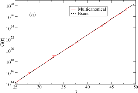
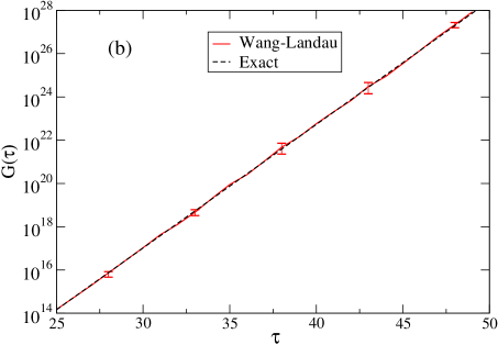
Figure 2: (Color online) Results of FHDMC for the case of fixed $\tau$ to the reduced polaron problem. Top: The results of FHDMC obtained with the application of multicanonicalberg . Bottom: The results of FHDMC obtained with the application of Wang-Landauwang algorithm for the same number of iterations (which approximately leads to the same CPU time). In addition, the exact results are shown for comparison.

Fig. 2 presents the results of our calculation of $G(\tau)$ for fixed values of $\tau$. The results of FHDMC were obtained with the application of multicanonicalberg (top of Fig. 2) and Wang-Landauwang (W-L) algorithm (bottom of Fig. 2) for the reduced polaron problem. We calculated $G(\tau)$ for $\tau=25.0,26.0,...,49.0$ and for approximately the the same amount of CPU time for comparison.

In our multicanonical simulation for a given value of $\tau$, our tolerance for the value of histogram of $I_{n}(\tau)$ for any $n$ was lower than twice and higher than half the value of the histogram for $I_{0}(\tau)$. Renormalization of the “density of states” was performed every $10^{5}$ iterations. After the histogram became flat within our tolerance, we carried out $3\times 10^{7}$ iterations for each instant of time considered. The total number of iterations required was $8\times 10^{8}$.

In our simulation using the W-L algorithm, we gave the modification factor $f$ the initial value $f=e$ and we reduce it according to $f_{i+1}=\sqrt{f_{i}}$ every time the histogram became “flat” within our tolerance. Our tolerance for “flatness” was such that the absolute value of the difference of the histogram $H_{n}$ for each value of $n$ from the average value of the histogram $\bar{H}$ to be less than $\bar{H}/10$. The “flatness” of the histogram was assessed every $10^{5}$ iterations. Choosing the final value for $f$ to be 1.000007629, the total number of iterations required was $8\times 10^{8}$.

Notice that both flat histogram algorithms yield $G(\tau)$ for any $\tau$ including very long-$\tau$ where $G(\tau)$ varies over many orders of magnitude. By fitting the long imaginary-time part of the Green’s function to a single exponential $G(\tau)=Ze^{-E_{0}\tau}$, we find that in the case of multicanonical the ground state energy is $E_{0}=-1.310\pm 0.004$ and $Z=0.88\pm 0.11$, while in the case of the W-L algorithm $E_{0}=-1.311\pm 0.004$ and $Z=0.88\pm 0.12$. The exact values are $E_{0}=-1.3146$ and $Z=0.77883$.

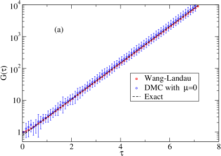
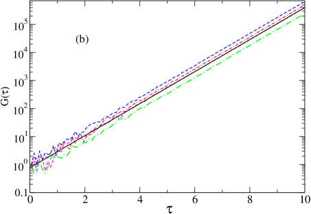
Figure 3: (Color online) (a) Comparison of the histogram of $G(\tau)$ obtained using the standard diag-MC, and the FHDMC. In addition, the exact $G(\tau)$ is shown for comparison. (b) The results of four different MC runs are compared with the exact results (solid line). See text for details.

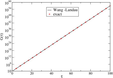
Figure 4: (Color online) Comparison of the exact histogram of $G(\tau)$ with that obtained using FHDMC using the WL algorithm to make the histogram flat. The error bars are too small to be seen on the present scale and have been omitted for clarity. Notice that we have used 2000 time intervals for the histogram.

Fig. 3(a) compares the results of our FHDMC for $g_{l}$ obtained with the W-L algorithm with the results of the standard implementation of the diag-MC without using the so-called guidance exponential function (i.e., parameter $\mu=0$). The simulation using the W-L algorithm was done as described earlier when discussing the results of Fig. 2 for the calculation of $G(\tau)$ for constant $\tau$. For comparison the diag-MC method was also applied for approximately the same CPU time. Notice that while the WL simulation gives results with negligible error bar (its size in this Figure is about the size of the symbols), the diag-MC calculation has significant errors. However, if we look closely we notice that the average values, from each time window to the next, do not fluctuate in a way which is consistent with the size of the error bar. In order to clarify this, we provide Fig 3(b), where the results of four different runs are presented (shown with different types of lines) where each curve is obtained using the same number of iterations starting from a different random initial configuration. Notice that, from one run to the other, the results for the histogram of $G(\tau)$ move in a correlated way (i.e., together) up or down and the four curves are parallel to each other for large values of $\tau$. The reason for that is the following. The exponential growth of $G(\tau)$ with $\tau$ makes $g_{n}>>g_{1}$ for large $n$. As a consequence of that the number of Monte Carlo steps “falling” in the first interval is relatively small. This means that the statistical fluctuations of the histogram height of the first interval are much larger than the statistical fluctuations of the histogram height of the other intervals. Within the diag-MC method the value of $g_{n}$ is obtained by simply multiplying the ratio of the corresponding histogram heights $H_{n}/H_{1}$ with the value of $g_{1}$, which is analytically known. Thus, due to these fluctuations, the value of $H_{1}$ is significantly different between two different MC runs and this affects the entire histogram by a multiplicative factor.

The problem discussed in the previous paragraph has been addressed by the standard diag-MC method when applied to the polaron problem by using an exponential guidance functionpolaronDMC1 . The diag-DMC, as has been applied in the polaron problempolaronDMC1 , uses the chemical potential as a “tunable parameter” to reduce the above mentioned statistical variance. In this particular problem, the exact asymptotic solution for $G(\tau)$ is a single exponential, $G(\tau)=Z\exp(-E_{0}\tau)$, where $E_{0}$ is the ground state energy. Therefore, using the chemical potential $\mu$, which corresponds to multiplying $G(\tau)$ by an exponential factor $\exp(\mu\tau)$ with $\mu$ as a tunable parameter, is effectively a simple way to make the histogram flat at long-$\tau$. The histogram becomes flat for the polaron problem simply when we choose $\mu\sim E_{0}$. If we use a value of $\mu$ close to $E_{0}$ this will improve the statistics of the diag-MC significantly. The closer the value of $\mu$ is tuned to the exact value of $E_{0}$, the better the diag-MC works. Therefore, in view of the present work, this works because such a guidance function makes the histogram of $G(\tau)$ approximately flat. However, this method of using such a guidance function is inferior to the present method because of the following reasons.

We do not a priori know the guidance function for more complex problems. An exponential decay of $G(\tau)$ with a single characteristic exponent is not the general rule in interacting many-body systems. In such systems, the general rule is that the Green’s function in imaginary time can be expressed as

$$G(\tau)=\int_{0}^{\infty}d\omega A(\omega)e^{-\omega\tau}$$ (20)

where $A(\omega)$ is related to the analytic continuation of the spectral function in imaginary time. Therefore, in general, we expect to need a continuum of such exponential energy scales. In most interesting systems it is not simple to extract $A(\omega)$ by the approach of tuning different exponential factors used in Ref. polaronDMC1 ; polaronDMC2 . The method presented here, however, constructs the exact “density of states”, with no a priori knowledge about it.

In order to further demonstrate the power of the present method, in Fig. 4 we present the calculated histogram of $G(\tau)$ in a detailed mesh of 2,000 intervals ranging from 0 to 100. This calculation took approximately 3 days of CPU time on a single 3 GHz processor. Notice that the agreement with the exact solution is excellent over approximately 60 orders of magnitude!

VI Conclusions

In conclusion, we have presented the FHDMC method to improve the standard diag-MC based on the idea of flat histogram methods. This idea was demonstrated on an exactly soluble problem, however, our method is very general and can be implemented for any problem where the diagrammatic MC method can be applied. We have shown with this method that the statistical fluctuations can be controlled even for very large values of the imaginary time without the need for any a priori knowledge about the behavior of $G(\tau)$.

References

- (1) N. V. Prokof’ev and B. V. Svistunov, Phys. Rev. Lett. 81, 2514 (1998).
- (2) A. S. Mishchenko, N. V. Prokof’ev, A. Sakamoto, B. V. Svistunov, Phys. Rev. B, 62, 6317 (2000).
- (3) E. Burovski, N. Prokof’ev, B. Svistunov, M. Troyer, Phys. Rev. Lett. 96, 160402 (2006).
- (4) K.-Y. Yang, E. Kozik, X. Wang, and M. Troyer, Phys. Rev. B 83 214516 (2011).
- (5) N. Prokof’ev and B. Svistunov, Phys. Rev. B 77, 020408 (R) (2008).
- (6) K. Van Houche, et al., Nature Physics, 8, 366 (2012).
- (7) L. Pollet, N. V. Prokof’ev, and B. V. Svistunov, Phys. Rev. B 83, 161103 (2011).
- (8) E. Kozik et al., Europhys. Lett. 90, 10004 (2010).
- (9) E. A. Burovski, A. S. Mishchenko, N. V. Prokof’ev and B. V. Svistunov, Phys. Rev. Lett. 87, 186402 (2001).
- (10) S. A. Kulagin, N. Prokofev, O. A. Starykh, B. Svistunov, C. N. Varney, Phys. Rev. Lett., 110, 070601 (2013). S. A. Kulagin, N. Prokofev, O. A. Starykh, B. Svistunov, C. N. Varney, Phys. Rev. B 87, 024407 (2013).
- (11) N. V. Prokof’ev, B. Svistunov, Phys. Rev. Lett. 99, 250201 (2007).
- (12) B. A. Berg, and T. Neuhaus, Phys. Lett. B, 267, 249 (1991).
- (13) P. M. C. de Oliviera et al., J Phys. 26, 677 (1996).
- (14) F. Wang and D. P. Landau, Phys. Rev. Lett. 86, 2050 (2001).
- (15) M. Troyer, S. Wessel, and F. Alet, Phys. Rev. Lett. 90, 120201 (2003).
- (16) E. Gull, A. J. Millis, A. I. Lichtenstein, A. N. Rubstov, M. Troyer, P. Werner, Rev. Mod. Phys. 83, 349 (2011), G. Li, W. Werner, and A. N. Rubstov, S. Base, M. Potthoff, Phys. Rev. B 80, 195118 (2009). E. Gull, Ph.D. Thesis.
- (17) H. Fröhlich, H. Pelzer, and S. Zienau, Phil. Mag. 41, 221 (1950).
- (18) R. P. Feynman, Phys. Rev. 97, 660 (1954).